Optimizing glassy $p$-spin models

Abstract

Computing the ground state of Ising spin-glass models with $p$-spin interactions is, in general, an NP-hard problem. In this work we show that unlike in the case of the standard Ising spin glass with two-spin interactions, computing ground states with $p=3$ is an NP-hard problem even in two space dimensions. Furthermore, we present generic exact and heuristic algorithms for finding ground states of $p$-spin models with high confidence for systems of up to several thousand spins.

I Introduction

Disordered materials, such as spin glasses, exhibit a rich equilibrium and nonequilibrium behavior. While the Edwards-Anderson Ising spin-glass model Edwards and Anderson (1975) incorporates the disorder and frustration required to replicate glassy behavior Young (1998), more generic models of disordered and glassy materials can provide insight into a number of related problems. In particular, spin-glass models with $p$-spin interactions have found a variety of applications across disciplines. They are excellent examples of disordered model systems in which the symmetry of the global states can be different from that of the local degrees of freedom.

For example, the mean-field theory of $p$-spin models with $p>2$ is closely related to the behavior of structural glasses Kirkpatrick and Wolynes (1987a, b); Kirkpatrick and Thirumalai (1987). The dynamics of mean-field $p$-spin models has a close similarity to mode-coupling theory Götze and Sjögren (1992) for the dynamics of supercooled liquids: Both the dynamical transition below which ergodicity breaking occurs and the thermodynamic transition below which replica symmetry breaking occurs (at the one-step level) Bouchaud et al. (1998) can be found in $p$-spin models Bouchaud et al. (1998). Because the study of models of interacting particles poses hard analytical and numerical challenges, there have been many efforts in modeling structural glasses and supercooled liquids using $p$-spin models Larson et al. (2010).

Similarly, there is a close relationship between implementations of topologically-protected quantum computing and $p$-spin models with disorder. To compute the error tolerance of topologically-protected quantum computing proposals the problem is mapped onto a statistical Ising spin-glass model with $p$-spin interactions Dennis et al. (2002). The point in the disorder–temperature phase diagram where the ferromagnetic–paramagnetic phase boundary crosses the Nishimori line Nishimori (1981) represents the error threshold—an important figure of merit—of the quantum computing proposal. For example, in the presence of bit-flip errors the Kitaev proposal Kitaev (2003) with four-spin interactions maps onto a two-dimensional random-bond Ising model (with $p=2$), the density of negative bonds representing the density of bit-flip errors. Topological color codes Bombin and Martin-Delgado (2007) instead map onto Ising spin-glass-like Hamiltonians with three-spin interactions in the presence of bit-flip errors Bombin and Martin-Delgado (2008); Katzgraber et al. (2009).

A common approach to better understand the low-temperature behavior of spin glasses is to study in detail the structure of the ground state: Zero-temperature optimization over the energetics of the system reveals properties of the finite-temperature thermodynamics of the system. This approach is complicated by the fact that these systems are, in general, NP-hard. This means that they belong to a large class of problems that are believed, in the worst case, to be solvable only by investing time exponential in the size of the problem Garey and Johnson (1979) (e.g., the number of spins). Elaborate techniques exist for solving NP-hard spin-glass optimization problems Liers et al. (2004); however, there are special cases, such as the two-dimensional Ising spin glass with $p=2$, that are not NP-hard, and where exact efficient optimization is possible Barahona (1982). Without disorder, the two-dimensional Ising model can be even solved exactly Onsager (1944), and techniques related to exact solutions of the pure model have been directly useful for producing efficient algorithms for simulating the two-dimensional Ising spin glass as well Saul and Kardar (1993); Loh and Carlson (2006); Thomas and Middleton (2009). Ground-state studies of two-dimensional spin glasses with $p=2$ have proven useful in many aspects of spin-glass theory, including chaos Bray and Moore (1987), reentrance Amoruso and Hartmann (2004), and nonequilibrium behavior Thomas et al. (2008). Although the two-dimensional pure Ising model with $p=3$ also permits an exact solution Baxter and Wu (1973); Baxter (1982), no efficient simulation techniques are known for the corresponding disordered problem.

Here we study the optimization of spin glasses with $p$-spin interactions. The optimization problem of finding ground states of a generic spin-glass with $p$-spin interactions is NP-hard. In contrast to the two-dimensional Ising spin glass with $p=2$, we show here that even the special case of the two-dimensional spin glass on any tripartite lattice with three-spin interactions is an NP-hard problem, at least for some disorder distributions. This is true despite the existence of an exact solution for the pure case Baxter and Wu (1973); Baxter (1982). The proof is based on a mapping of the three-dimensional $p=2$ Ising spin glass—which is known to be NP-hard—onto the two-dimensional $p=3$ Ising spin glass. Nevertheless, we present an approach that is capable of computing exact ground states of the three-spin model for moderate-sized systems. While the exact approach presented has been developed specifically for three-spin interactions, it can be generalized to other values of $p$. We also present a heuristic approach that works quite well for systems of up to several thousand spins. This technique is general: The same code may be used to optimize a spin-glass problem with any geometry and any value of $p$. It consists of a genetic algorithm using triadic crossover Pal (1994) combined with a local search.

In Sec. II we outline details of Ising models with three-spin interactions, followed by a proof that the disordered three-spin Ising model is NP-hard. We then present optimization techniques to study models with $p$-spin interactions in Sec. IV followed by some results on test instances in Sec. V.

II Disordered three-spin Ising model

The standard Edwards-Anderson (EA) spin-glass model with two-body interactions is given by the Hamiltonian

$$\mathcal{H}_{\mathrm{EA}} = -\sum_{\langle ij\rangle}J_{ij}s_{i}s_{j},$$ (1)

where the sum is over all nearest-neighbor pairs $\langle ij\rangle$. The Ising spins $s_{i}\in\{\pm 1\}$ interact via random couplings $J_{ij}$. The three-spin model, on the other hand, has spins placed on the vertices of a triangulated lattice with plaquette interactions $J_{ijk}$ between the spins $i$, $j$ and $k$ on each plaquette $\triangle_{ijk}$. The Hamiltonian is

$$\mathcal{H}_{3} = -\sum_{\triangle_{ijk}}J_{ijk}s_{i}s_{j}s_{k}.$$ (2)

A plaquette is said to be unsatisfied when its contribution to the Hamiltonian is positive. Typically, this model is studied either on a triangular or a Union Jack lattice.

Both the triangular and Union Jack lattices are tripartite: One can assign one of three colors to each site of the lattice such that neighboring sites never have the same color; i.e., there are three colored sublattices. This model is most convenient to work with on a tripartite lattice. In this case, all spins border an even number of plaquettes (see the left-hand side of Fig. 1). Furthermore, each pair of spins shares an even number of plaquettes (zero or two), so the spins appear together in an even number of terms in the Hamiltonian. Flipping a spin therefore alters the satisfaction of an even number of plaquettes adjacent to each spin. All configurations of the system can be composed of individual spin flips, so the set of plaquettes with differing satisfactions between any two spin configurations must contain an even number of plaquettes touching each spin. For a three-spin Ising model on any tripartite lattice, this gives a conservation rule: The parity of the number of unsatisfied plaquettes touching each spin depends only on the instance of disorder. While for the EA Ising spin glass with $p=2$ frustration properties are associated with the plaquettes, in the three-spin model this conservation rule imparts frustration properties to the sites of the spin lattice. If the number of unsatisfied plaquettes touching some spin is even for some configuration, then it is even for all spin configurations, and if it is odd for some configuration, then it is frustrated in that there is no configuration which has zero (or any even number of) broken plaquettes touching this spin. In particular, if all spins are unfrustrated, then the partition function is identical to that of the pure system.

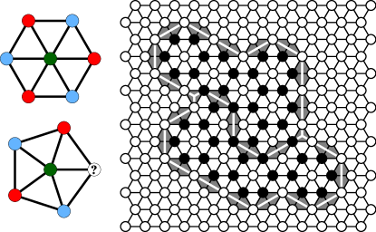
Figure 1: (Color online) On a triangulated tripartite lattice each spin touches an even number of triangular plaquettes (top left). If a spin touches an odd number of triangular plaquettes (bottom left), there is no three-coloring of the graph, in contradiction with the assertion that the graph be triTartite. Right panel: A section of a three-spin system showing a domain wall separating states of the system. White (black) circles show spins that are aligned (anti-aligned) with some reference configuration. White plaquettes correspond to terms that contribute identically in this new spin configuration as in the reference configuration, while the gray plaquettes correspond to terms with opposite sign to that of the reference configuration. To guide the eye, the domain walls are highlighted with white lines, separating two states of the system. Unlike in the Ising spin glass with $p=2$, three different states may come together at a point; thus the system cannot be described entirely in terms of domain-wall loops.

Each term of the Hamiltonian in Eq. (2) involves three spins which are adjacent to one another, so each spin is a member of a different color sublattice. Unlike in standard spin-glass problems, global spin-flip symmetry is absent: Flipping all spins negates the Hamiltonian, rather than leaving it unchanged. There is instead a four-fold symmetry in the model from flipping all the spins on certain colored sublattices. Flipping all the spins on any two of the three colored sublattices leaves every term of the Hamiltonian unchanged, so that the model is four-fold degenerate. At low temperatures, these four degenerate states make up domains of the system, with domain-wall excitations separating the pure state regions. In the two-dimensional Ising spin glass with $p=2$ Thomas and Middleton (2007), the boundaries between different states can be expressed entirely in terms of the domain-wall loops. In the three-spin model, a similar loop description may be used to describe the domain-wall separation between any two domains: The loops connect only sites on the same sublattice, and any plaquette the loop crosses is a member of the domain wall. The loop description is incomplete in this model, because it is possible to have three different states come together at a point (see the right-hand side of Fig. 1). In this sense, and because of the four-fold symmetry of the model, the Ising model with three-spin interactions closely resembles a four-state Potts model. Despite the presence of domain walls that cannot be classified as loops, a loop description of the problem will be a useful limiting case to consider. This loop description is helpful for proving the three-spin ground-state problem is NP-hard and for developing an optimization algorithm for this ground-state problem.

III The three-spin model is NP-hard

While instances of the bond-disordered Ising model with two-body interactions in two dimensions may be solved exactly (i.e., find a ground-state configuration or compute the partition function) with efficient algorithms, the same model in three space dimensions is NP-hard Barahona (1982). We show here that the two-dimensional three-spin Ising model is NP-hard as well by constructing a polynomial mapping by which three-dimensional spin-glass ground states may be found using specially-constructed instances of the two-dimensional three-spin model.

First, we examine the Ising spin-glass model with $p=2$. In two dimensions, there is a one-to-one correspondence between spin configurations and polygonal structures on the dual lattice, the sets of domain-wall loops. These polygons cross the bonds that are broken, relative to some reference configuration Thomas and Middleton (2007, 2009). Therefore each state of the Ising model corresponds to a state of the loop model with the same energy, and the converse is also true: The models are equivalent and have the exact same physical properties. In two dimensions, the lowest-energy loop configurations may be found by mapping the problem to a minimum-weight perfect matching problem on a related (nonbipartite) lattice. Minimum-weight perfect matchings may be solved efficiently using Edmonds’s blossom algorithm Edmonds (1965) (with subsequent fast implementations Cook and Rohe (1999); Kolmogorov (2009)).

The correspondence between domain-wall configurations and spin configurations is exact in any space dimension; i.e., a similar construction may be made in general. In three dimensions, the domain-wall structures are polyhedra: sets of two-dimensional surfaces. The energy of the system is given by the sum over all faces in each set of polyhedra. Each face of the domain-wall polyhedra crosses one edge from the spin lattice. The faces of these polyhedra are defined on a polyhedral graph, another cubic lattice with one node at the center of each cube of the spin graph. The polyhedral graph is closely connected with the spin graph: Each face of the polyhedral graph crosses one edge of the spin graph, while each edge in the polyhedral graph is in turn crossed by one face of the spin graph. A wire-frame graph may also be defined that will be convenient for specifying the set of domain walls that correspond to one spin configuration. Each node of this wire-frame graph corresponds to either a face or an edge of the polyhedral graph (all faces and edges are represented). The graph is bipartite: The nodes corresponding to a particular face (edge) of the domain wall graph are connected to the nodes corresponding to the edges (faces) touching this face (edge). Note that, because the faces (edges) of the polyhedral graph correspond to the edges (faces), this wire-frame graph is also defined on the faces and edges of the spin graph. A small subset of the polyhedral graph and the corresponding elements of the wire-frame graph is shown, for example, in Fig. 2.

We now specify the energetics of the spin system in terms of the domain walls on the polyhedral graph. Start by defining a reference spin configuration ${r_{i}}$. For each bond among nearest-neighbor pairs $\langle ij\rangle$, let $R_{ij}\equiv r_{i}r_{j}$. For a face $f$, which crosses the bond between sites $i$ and $j$, let the weight $w$ be defined by $w(f)\equiv 2J_{ij}R_{ij}$. Then the Hamiltonian may be rewritten

$$\mathcal{H} = -\sum_{\langle ij\rangle}J_{ij}\left(s_{i}s_{j}-R_{ij}+R_{ij}\right)$$ (3)

$$= \mathcal{H}_{R}+\mathcal{H}_{P},$$

where $\mathcal{H}_{R}\equiv-\sum_{\langle ij\rangle}J_{ij}R_{ij}$ is the constant contribution of the reference configuration and $\mathcal{H}_{P}\equiv-\sum_{\langle ij\rangle}J_{ij}\left(s_{i}s_{j}-R_{ij}\right)=\sum_{f\in P}w(f)$ is the contribution from a polyhedral structure $P$ corresponding to the domain wall separating configuration ${s_{i}}$ from ${r_{i}}$. When $\mathcal{H}_{P}$ is minimized, so is $\mathcal{H}$.

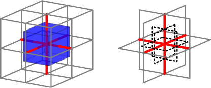
Figure 2: (Color online) Simplest possible relative domain wall for the three-dimensional Ising spin glass. On the left, one spin, in the middle, is flipped relative to a reference configuration, changing the bonds which are drawn thicker (and shown in red), and imposing the domain-wall polygon (the shaded cube in the center, here blue). The dashed lines shown on the right are the intersections of this surface with the plaquettes (faces) of the cubic lattice. This projects the domain wall onto a wire-frame representation, which will be useful for mapping onto the three-spin problem. Only the plaquettes that intersect the domain wall are shown. In general, each plaquette touches an even number of these dashed edges, while each edge touches either zero or four of them.

These polyhedral structures may be uniquely defined by a wire-frame representation: Here each face of the polyhedral graph is replaced by the intersections of the polyhedra with the faces of the original spin lattice, the graph given by the spins and their interactions, as is shown in Fig. 2. In this representation, each edge $e$ sits on a face $f_{e}$ of the polyhedral structure $P$, and has weight $w(e)=w(f_{e})/4$, so that $\mathcal{H}_{P}=\sum_{f\in P}w(f)=\sum_{e\in P_{e}}w(e)$. The set of edges $P_{e}$ corresponding to the set of faces $P$ making up a valid polyhedral set has two constraints. First, when four edges meet at the center of a single face on the polyhedral graph (at an edge of the spin graph), then the face must as a whole be selected or not, so either none of the edges is included, or all four are. We call these “type 1” constraints. Second, when four edges meet at the center of a face of the spin graph, these are the edges on the polyhedral graph, and any even number of these edges may be included to give a valid polygon. We call these “type 2” constraints. In Figs. 3 and 4, the square junctions follow the first constraint, while the circle junctions follow the second constraint. This defines the set of all polyhedral structures that are equivalent to the three-dimensional Ising spin glass model.

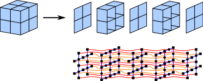
Figure 3: (Color online) The three-dimensional Ising model on a cubic lattice (spins sit at the vertices of the cubic lattice) is split into slices. The intersection of a domain-wall surface with the faces and edges of the graph uniquely defines the spin configuration. Below, the graph is converted to a wire-frame form where the set of all spin configurations is equated with the set of all selections of edges where squares (corresponding to edges of the cubic lattice above) are type 1 junctions, which always touch either zero or four of the selected edges. Circles—corresponding to faces of the cubic lattice above—are type 2 junctions, which always touch an even number of selected edges. The edges are allowed to cross (crossing edges correspond to a type 0 junction). Colors are used to guide the eye.

This wire-frame description may be drawn sliced into segments, as shown in Fig. 3; edges are allowed to cross, as is necessary if one is to embed a three-dimensional graph in two dimensions. Crossing edges must not interact with one another, introducing one more junction (type 0). Zero or four of the edges that come together may be included, or two edges opposite one another, but no turns are allowed. This is shown in Fig. 4.

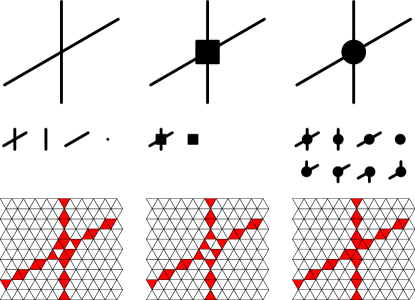
Figure 4: (Color online) Junctions used in the mapping from the graph in Fig. 3 to the three-spin model. Top: The junction type is shown as a crossing with no symbol (type 0), square (type 1), and circle (type 2). Below the junctions is an enumeration of all possible edge selections for each junction. Bottom: The junction is represented as a plaquette disorder distribution. White plaquettes are given prohibitively large weights such that they may not flip. The only remaining spin configurations correspond to flipping the plaquettes on paths according to the rules above. The shaded (red) plaquettes all have zero weight, except for one arbitrarily chosen plaquette in each square junction, which is given the weight of the face of the polygon it corresponds to.

With three types of junctions, this wire-frame graph may be embedded in the two-dimensional glassy three-spin model. We take the wire-frame graph, as drawn in Fig. 3, and replicate each item of the graph by setting the three-spin interactions $J_{ijk}$ of the spin problem as appropriate. One of the colored sublattices (as defined in Sec. II) of the three-spin model is chosen to house all the domain walls in this graph. This is enforced by setting bulk plaquette weights (i.e., the weights of all plaquettes that are not allowed to be in a domain wall or in a junction) to be prohibitively large, such that they must be satisfied in the ground state. In Fig. 4, these bulk plaquettes are colored white; they make up the domains for which the domain-wall loops separate. Each edge of the wire-frame graph is mapped to a zero-energy domain-wall segment: a set of plaquettes with zero weight, but surrounded by bulk plaquettes so that any valid spin configuration has either all or none of the plaquettes unsatisfied (in the case of a zero-weight plaquette, we choose to use the terms satisfied and unsatisfied as though it had positive weight). Finally, the three types of junctions are replaced by the three types of plaquette “cities” shown in Fig. 4, which are consistent only with spin configurations that produce satisfactions in the domain walls so that they interact with one another in exactly the ways the edges in the wire-frame model are constrained to interact. The weights of the plaquettes in the cities are all zero, except in each square junction, where one plaquette is chosen to have the weight of the face in the corresponding polyhedral model. As either all or none of the plaquettes in this junction are satisfied, it does not matter which plaquette is given the nonzero weight.

The sum of the weights of all the bulk plaquettes does not depend on the weights in the wire-frame model, so it is a constant, $\mathcal{H}_{c}$. The sum of the weights of the remaining (domain wall and junction) plaquettes depends only on the satisfaction of each square junction, as all other plaquettes have zero weight. Therefore the Hamiltonian $\mathcal{H}_{3}$ of the three-spin model with these plaquette weights may be written in terms of the polygonal structure $P$ as

$$\mathcal{H}_{3} = \mathcal{H}_{c}+\sum_{f\in P}w(f)-\sum_{f\notin P}w(f).$$ (4)

Calling $\mathcal{H}_{f}=\sum_{f}w(f)$ a disorder-dependent constant related to $\mathcal{H}_{R}$, we obtain

$$\mathcal{H}_{3} =\mathcal{H}_{c}+\mathcal{H}_{f}+2\mathcal{H}_{P}$$ (5)

such that

$$\mathcal{H} =\mathcal{H}_{R}-\frac{1}{2}\mathcal{H}_{c}-\frac{1}{2}\mathcal{H}_{f}+\frac{1}{2}\mathcal{H}_{3}.$$ (6)

Because $\mathcal{H}_{R}$, $\mathcal{H}_{c}$, and $\mathcal{H}_{f}$ are all constants that may be computed efficiently for each instance of the disorder, this directly relates the ground state of a specific instance of the two-body three-dimensional Ising spin glass to a specific instance of the two-dimensional three-spin model.

The number of spins necessary in the three-spin model is polynomial in the number of spins in the three-dimensional Ising spin-glass problem. This is because the only constraint forcing the number of spins in the three-spin model to scale faster than linearly with the number of spins in the three-dimensional Ising spin glass model is that a new junction must be created for each crossed edge. If we assume the worst scaling possible, i.e., that the length of every domain wall must scale linearly with the total number of domain walls in the problem, then the number of spins necessary in the three-spin model is bounded from above by $\mathcal{O}(N^{2})\times\mathcal{O}(N^{2})=\mathcal{O}(N^{4})$, for $N$ spins in the three-dimensional Ising spin glass, which is still polynomial. As the ground state of any three-dimensional two-body Ising spin glass may be found by solving an instance of the two-dimensional three-spin model ground-state problem with a number of spins polynomial in $N$, finding the ground state of this three-spin model is NP-hard.

IV Optimization methods for $p$-spin models

The three-spin spin-glass model is NP-hard, so it is unsurprising that we have not found any fast (i.e., polynomial run time with system size) exact algorithm for computing ground states. We start by describing an exact integer linear program (ILP) technique for optimizing the three-spin glassy model using cutting planes. This technique scales exponentially with the system size to find exact results, but it is particularly useful because one may quickly find tight lower bounds on the ground-state energy. We then present an efficient heuristic technique for arbitrary $p$ using the triadic crossover genetic update of Pal Pal (1994), with which we can solve, with high confidence, systems with discrete disorder up to several thousand spins.

IV.1 Cutting plane technique (exact algorithm)

Ground states of the Ising spin glass have been computed using ILP approaches Barahona et al. (1988); Liers et al. (2004). Here we show that the three-spin model may also be optimized exactly by mapping the problem onto an ILP combined with a cutting-plane technique. This approach does not depend on the distribution of disorder, and its performance is roughly comparable for Gaussian and bimodal disorder.

An ILP may be expressed in canonical form with coefficient vectors $c$ and $b$, coefficient matrix $A$, and vector $x$ of integer variables as

Minimize $$c^{T}x$$ (7)

Subject to $$Ax\leq b.$$

The function to minimize, $c^{T}x$, is called the objective function; the elements of $Ax\leq b$ are the constraint inequalities. The problem is specified by giving the values of all elements of $A$, $b$, and $c$. The function $c^{T}x$ is, up to a linear transformation, equal to the Hamiltonian to be minimized, while each row of the constraint inequality equation is a constraint on the values of the plaquettes designed to enforce that only valid spin configurations are allowed (the number of rows of $A$ and the number of elements of $b$ is the number of constraints in the linear program). An optimal vector $x$ gives the lowest value of the objective function among all possible $x$ that satisfy the constraints. This problem is often posed as a maximization problem; this is equivalent, as one may replace $c$ with $-c$ and solve the maximization problem. Typical linear program solvers can optimize in either direction.

Solving an ILP is an NP-hard problem, but linear programs without the integer constraints permit efficient solutions, e.g., by simplex or interior point methods Chvátal (1983). It is therefore possible to solve ILPs by successively adding cutting planes to linear programs: Additional constraints are added to enforce that the solution vector $x$ contains only integers. This can be achieved by constructing a tight convex hull around the permitted values with intersections only at permitted integer values. This tight hull requires exponentially many constraints to specify, so in practice one tries to find and add only the most important extra constraints.

For both the two-body Ising spin glass and the three-spin spin-glass model, the Hamiltonian is not linear in the spin degrees of freedom. Therefore, expressing the problem as an ILP requires additional work. One may perform a change of variables such that the Hamiltonian is linear in the new variables. For the Ising spin-glass problem, the Hamiltonian is quadratic in the spin degrees of freedom, so the Hamiltonian is a weighted sum of edge satisfactions $e_{ij}\equiv s_{i}s_{j}$. The spin values are uniquely defined by the edge satisfactions, up to a global spin-flip degeneracy. In the three-spin case, the Hamiltonian is linear in three-spin plaquette terms $x(\ell)\equiv s_{i}s_{j}s_{k}$ where plaquette $\ell$ touches spins $i$, $j$ and $k$. The vectors $x$ and $c$ therefore are of size $N_{p}$, the number of plaquettes in the system, and for each plaquette $\ell$ defined as above, $c(\ell)=J_{ijk}$. Performing a linear transformation on the plaquette satisfaction variables from $x(\ell)\in\left\{-1,1\right\}\rightarrow x(\ell)\in\left\{0,1\right\}$ optimizes the new Hamiltonian $\mathcal{H}_{\mathrm{LP}}=(\mathcal{H}+N_{p})/2$, for which the optimization problem is equivalent, and which trivially maps back to the original problem. The spin values may be extracted by changing variables back to the original spin degrees of freedom; the configuration is determined only up to the four-fold degeneracy of the model, so two spins (preferably adjacent to one another) may be assigned randomly, and this forces the values of all other spins.

As in the spin-glass case, the change of variables to reduce the cubic program to a linear program moves the complexity of the optimization problem from the cubic objective function, which produces a very complex energy landscape (but with no constraints besides the variables being integers), to a linear objective function, which has additional constraints to ensure that the two formulations are equivalent. The extra constraints are necessary because not all plaquette configurations correspond to a valid spin configuration. The constraints to be added are a generalization of the odd-cycle (OC) constraints used in the spin-glass technique.

The parity conservation rule introduced in Sec. II implies a related principle: The number of plaquettes whose satisfaction differ between any two spin configurations must be even. This can be seen by changing from one spin configuration to the other one spin flip at a time. No spin flip can change the parity, so it is always even. Furthermore, the interaction of any loop on one of the colored lattices (using the representation in Fig. 1) with any spin configuration has the same parity constraint. In the bulk of the sample, this constraint is implied by the previous one, but when the system has periodic boundaries, it adds the case of system-spanning loops, which do not correspond to spin configurations. The inclusion of these system-spanning loops ensures that the solution is in the correct topological sector, which is necessary for the spin configuration to be well defined when converting from plaquette values to spin values (c.f. the extended ground state in spin glasses Thomas and Middleton (2007)).

These parity constraints lead to OC-like inequalities. Let $\mathcal{C}$ be a set of objects for which the vector $x$ has $N_{p}$ elements given by the union of the set of all spin-configuration differences with the set of all loop differences (as defined in Sec. II) with a spin configuration. These objects can be defined by the vector $x$ which gives (possibly fractional) plaquette satisfactions. For each member $C\in\mathcal{C}$, all $F\subset C$ with $\left|F\right|$ odd satisfy

$$x(F)-x(C\setminus F)\leq\left|F\right|-1.$$ (8)

Each such equation rules out the case where $\forall\ell\in F,x(\ell)=1$ and $0$ otherwise – with $|F|$ odd, this is not allowed by the parity constraint. Thus this set of constraint inequalities provides the cutting planes to eliminate invalid solutions. Clearly, the number of constraints is huge: Every possible spin configuration contributes many constraints of this type to the linear program, so it is unreasonable to include them all. It is therefore necessary to find the most important constraints without which the solution is incorrect and ignore as many others as possible, i.e., such that $A$ and $b$ are not too large. If too few constraints are included at a given step, the solution given by the linear program at that step will not correspond to a valid spin configuration. It will have energy lower than the ground-state energy because the problem is underconstrained (adding new constraints can only raise the value of the solution).

Given a test solution where the linear program solution contains either odd-plaquette violations or non-integer variables (typically both), one searches for new constraints that are violated by the current configuration. These are added to the problem, and the linear program is solved again. This is repeated until the result is a valid plaquette configuration, in which case all constraints are satisfied (including the integer variables condition). Also, for discrete disorder distributions, the solution is complete if the lower bound given by this technique is close enough to confirm that a heuristic solution is an exact solution.

If adding constraints does not produce a solution to the ILP, one may also branch: Assign the values of one or more variables, and search given these variables. The full solution requires exhausting the exponentially-many possibilities, but some of these possibilities can be eliminated if both good upper and lower bounds can be computed for the cases. Many practical frameworks exist for combining branching with cutting planes. For the implementation of the algorithms described here, we use the Coin Branch and Cut (CBC) framework with the Coin Linear Program Solver (CLP) simplex algorithm to solve individual linear programs coi .

We outline the procedures used for finding new constraints step-by-step:

• Local spin-flip constraint finder — The simplest sets of constraints involve $C$ being the six plaquettes adjacent to a given spin. With $2^{|C|-1}=32$ possible choices of $F$, all possible constraint violations may be tested around each spin, although this is typically unnecessary: It is often simple to identify which combinations are most likely and test only those (for example, in the case where all weights are currently integers, adding the $x=1$ cases and subtracting the $x=0$ cases is the only one of the 32 which can produce a violated constraint). The simplest generalization of the local spin-flip constraint finder is taking the plaquettes that change when flipping multiple nearby spins. We have tried all combinations of up to four spins. These help the convergence of the ILP only marginally. Therefore they are only included as a last resort check if all other constraint finders fail.

• Loop constraint finder — In analogy with the constraint finders for the Ising spin glass presented in Ref. Barahona et al., 1988, one can use all the finders used for loops in the Ising spin glass on the loops of the tripartite sublattices. The major difference is that each edge in the loop description of the three-spin model contains two plaquettes. This actually simplifies some aspects of the computation because all loops are guaranteed to have even length. Two constraint finders, the spanning tree heuristic for odd cycles (SHOC) and the shortest paths exact finder, odd-cycle (OC) in Ref. Barahona et al., 1988, are particularly useful for our application, although any constraint finder from the spin-glass problems could be similarly ported to the three-spin problem. Some of these constraint finders will naturally produce some even-cycle violated “constraints” that are not valid because all constraints must contain an odd number of items in $F$. These are normally discarded, but it is useful to store them for later use in the genetic constraint finder below.

• “Worm” constraint finder — All the constraint finders for the ILP solution of the Ising spin glass work with loops; this is not the only kind of constraints available in the three-spin model; i.e., another class of finders is also needed. One approach employed to find nonloop constraints is to do a search by flipping adjacent spins successively. At each step of the search, we keep the set of flipped spins and the direction in which the set of spins (the “worm”) is growing. Four possibilities are considered: capping the worm and testing if it produces a valid constraint, or letting the worm grow straight or turn to the left or right. If the worm is to grow, the weights of the two new plaquettes are recorded. For each plaquette $\ell$, if $x(\ell)<0.5$, one adds $x(\ell)$ to the total weight so far, otherwise add $1-x(\ell)$. If the total weight so far ever exceeds $1$, the search may stop because no constraint found after this point can satisfy a constraint in the form of Eq. (8).

• “Genetic” constraint finder — If the above constraint finders are insufficient, we have developed one additional powerful constraint finder. Any spin configurations may give valid constraints, and finding the tightest convex hull is very difficult, even with the highly-effective constraint finders outlined above. Additional constraints may be found by combining sets of plaquettes from different constraint inequalities using a symmetric difference. In the case where the two constraint inequalities contain at least one common variable, the new inequalities are not simply a linear combination of the two previous ones, so they exclude a different region of parameter space and may be useful. It is particularly helpful when the cases where $|F|$ is even are kept in the above constraint finders, because one is most likely to find a constraint inequality with $|F|$ odd when combining an odd case with an even case. In practice, these often produce new constraint inequalities that are violated. We call this a genetic constraint finder because it takes the population of currently known constraint inequalities, all of which might be satisfied by the current configuration, and it generates new constraint inequalities (better offspring) by combining two constraints at random. This constraint finder would also allow one to find new constraints in ILP solutions of the Ising spin glass.

The exact technique presented here depends on finding good constraint inequalities; the machinery for finding these inequalities is more developed for quadratic programming, so we have developed a partial reduction technique to take advantage of this (the loop constraint finder) in addition to our constraint finders, which work directly with the three-spin problem. This reduction is highly influenced by the geometry of the problem, which makes it effective for finding good constraints. Buchheim and Rinaldi have also recently developed a different technique that fully reduces a cubic programming problem to quadratic program Buchheim and Rinaldi (2007). This reduction does not take advantage of known geometrical constraints, but it has the substantial advantage that it would eliminate the need for the more specialized constraint finders, allowing one to use only quadratic programming techniques to solve the problem. It would be interesting to compare these two methods for solving this ground-state problem.

IV.2 Local search optimization

We describe a simple generic local search algorithm. It is similar to standard local search optimization methods Martin (2004). While it is not particularly effective for continuous disorder distributions (in that case a variable-depth search performs better), it works quite well for the case of discrete disorder. This local search algorithm has been designed with the three-spin problem in mind, but it is generic: It works well for all the spin systems we have tried when they have discrete energy levels, regardless of space dimension or the value of $p$. It consists of a depth-first search where at each step in the search a spin is test-flipped and the search may overcome energy barriers up to some cutoff energy. It is most easily implemented with a boolean recursive function. In all, $N$ searches are run, one starting from each spin in the system, in random order, for a given cutoff search depth $d_{\mathrm{max}}$ and energy barrier $E_{\mathrm{max}}$ to overcome. One of these searches is implemented by calling, for site $i$, searchstep$(0,i)$, where this is the boolean function defined by

boolean function searchstep$(d,i)$
if $d>d_{\mathrm{max}}$
return false
flip $s_{i}\leftarrow-s_{i}$
if $E(\{s_{i}\})<=E_{\mathrm{max}}$
if $E(\{s_{i}\})<=E_{\mathrm{t}}$
return true
for each $j$ which neighbors $i$
if searchstep$(d+1,j)$ returns true
return true
reset $s_{i}\leftarrow-s_{i}$
return false

When the function returns true, the energy has been lowered by switching to a new spin configuration. When it returns false, no change has been made to the spin configuration. For bimodal disorder, this procedure typically finds the true ground state in small systems of up to $\sim 300$ spins ($L\leq 18$ in two space dimensions), when $d_{\mathrm{max}}>L$ and $E_{\mathrm{max}}$ is given by twice the smallest energy increment in the system. It is also a useful search technique for the genetic algorithm described in the next Section.

IV.3 Genetic algorithm with local search

Genetic algorithms are useful heuristic techniques for solving optimization problems with complex energy landscapes. A genetic algorithm consists of a population of solutions—many distinct instances of the problem that eventually evolve toward the solution of the optimization problem. One way for a genetic algorithm to proceed is that at each step of the algorithm parent instances are chosen and reproduced: The offspring (or child instances) are generated by combining the parent solutions in some way and the children are added to the population. Some members of the population are eliminated according to a fitness criterion to keep the population size from growing.

In order for a genetic algorithm to be effective, there must be an efficient mechanism for reproduction: Child solutions must be as fit as their parents, or they are likely to be eliminated soon, although there must be enough variation such that child solutions are not simply repeats of previous members of the population. One effective reproduction mechanism for spin systems is triadic crossover Pal (1995, 1996). Like in standard crossover reproduction, the bits of two children are created by swapping bits of two parents. In this case, which parent’s bit goes to which child is decided by comparing one of the parents with a third parent. When the spin values in parents 1 and 3 are equal, child 1 inherits the spin value from parent 1, while child 2 inherits the spin value from parent 2. When the spin values differ between parents 1 and 3, child 1 inherits the spin value from parent 2, and child 2 inherits the spin values from parent 1.

Other than the Hamiltonian, which spatially couples the spins, the triadic crossover technique does not use the spatial structure (good regions of spins to flip are chosen solely from their correlation among different instances) so storing each spin as one bit and using bitwise operations on strings of bits significantly decreases both the storage space necessary and the number of operations necessary to perform the steps of this algorithm.

Pal originally used the triadic crossover technique with only very simple randomized local optimization techniques. Triadic crossover has also been exploited in conjunction with highly-sophisticated optimization procedures to find heuristic ground states in the three-dimensional Ising spin glass up to $14^{3}$ Hartmann (1997). We employ an intermediate approach: The local optimization algorithm from the previous subsection is quite simple but performs very well. At each step of the genetic algorithm we perform a triadic crossover reproduction to produce two child instances from three randomly chosen parents. Each of these child instances is then optimized by a single local search sweep (starting once from each spin in the system, with a depth cutoff of $L$). Then, each child is compared against a randomly chosen instance in the population with fitness below the median (energy above the median of the whole population). If the child’s fitness is better, it may replace this randomly chosen instance. To keep the population heterogeneous, we allow this replacement only if the child is not a repeat of any current member of the population. No additional randomization is carried out in this procedure. This is adequate for some cases (such as the Ising spin glass results presented below), while in other cases it helps to carry out parallel evolution starting from several different initial populations to increase heterogeneity.

We have produced a highly portable code which is effective for systems of up to several thousand spins (performance is similar to that of the highly-sophisticated code in Ref. Hartmann, 1997). The simplicity of this technique makes it particularly convenient to port to different types of interactions: We can use the same code to optimize the two-dimensional and three-dimensional Ising spin glass, the Sherrington-Kirkpatrick (mean field) Ising spin glass, as well as for arbitrary $p$-spin models.

IV.4 Combining the techniques

While the exact solution of the three-spin problem using the ILP solution is quite time consuming for more than $\sim 300$ spins, the cutting planes technique quickly provides an exact lower bound on the ground-state energy that is often very close to the true ground state. It is common to use heuristic solutions as a part of a branch-and-cut technique Liers et al. (2004); in cases of discrete disorder, in particular, the ILP lower bound is quite commonly below the heuristic solution by less than the energy of a single spin flip. The heuristic ground state solution is therefore shown to be exact. For a system with $3$-spin interactions and $24^{2}$ spins, we find that the solution can be confirmed exact in a reasonable amount of time in $95\%$ of the samples. In the other cases, it is likely that the heuristic solution is still correct, but we have not proven it with this technique.

V Genetic algorithm results

This algorithm is intended for use on $p$-spin models for any $p$, but it is difficult to test its performance in these models because there are no exact techniques known for the optimization of large instances of $p$-spin models. To study the performance of the algorithm, we therefore use the two-dimensional Ising spin glass with $p=2$, followed by some tests on the three-spin case. We then compute the ground-state energy per spin $E_{0}/L^{2}$ for the disordered Ising model with $p=3$ on a triangular lattice.

V.1 Benchmark case: Ising spin glass ($p=2$)

Fast algorithms for optimizing the two-dimensional Ising spin glass with $p=2$ are readily available Barahona (1982); Thomas and Middleton (2007); Pardella and Liers (2008); Liers and Pardella (2010), so we can find the parameters for which the genetic algorithm does produce correct solutions with high confidence. We use the Ising spin glass with bimodal interactions; bond values are chosen to be $1$ or $-1$ with equal probability. For simplicity, we compare against cases where the ground state is equal to the extended ground state Thomas and Middleton (2007); these ground states are expected to behave as the other ground states, so that this choice should not affect the performance results significantly. For a given population size $N_{p}$, we find the probability that the genetic algorithm gives an incorrect result, as shown in Fig. 5. For $N_{p}\geq N$, with $N$ being the number of spins, these errors are very rare up to rather large system sizes; for $N_{p}=4N$, we failed to find any errors for $L<50$ in $2\times 10^{4}$ attempts, while for $N_{p}=N$, the same is true for $L<40$.

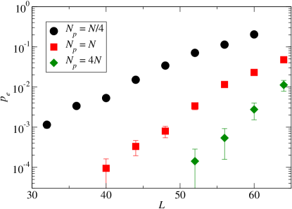
Figure 5: (Color online) Probability $p_{e}$ that the genetic algorithm described in Sec. IV.3 gives an incorrect ground state for the two-dimensional Ising spin glass with $\pm J$ disorder and $p=2$. Increasing the population size allows for more genetic variation, such that the algorithm is able to find the true ground states of large systems. No parallel runs are performed to further increase variation in this case. Where the statistical error bars are not visible, they are smaller than the symbols.

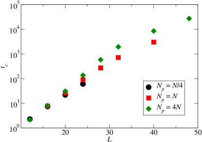
Figure 6: (Color online) Number of steps $t_{c}$ necessary to find the lowest-energy state (in the cases where the true ground state is actually found) for the two-dimensional Ising spin glass with $\pm J$ disorder. If more than one error has occurred at a given system size $L$ (see Fig. 5), the solution technique is presumed ineffective at $L$ and the data point is omitted. The time required to find the correct result scales exponentially with $L$ for the system sizes studied, however with a small enough prefactor to make these computations reasonable up to $L\approx 50$. Statistical error bars are smaller than the symbols.

For the two-dimensional Ising spin glass, the local search algorithm is quite effective, so for small systems, it takes few updates to find the true ground state. For larger systems the number of updates necessary to reach the true ground state in a two-dimensional Ising spin glass with $p=2$ scales exponentially (or at least as a power law with exponent $>6$). In Fig. 6, the number of reproduction steps necessary to reach the true ground state is plotted in the cases where the true ground state can actually be reached; when the true ground state is unreachable for some samples, we exclude the run-time data.

V.2 The disordered Ising model with $p=3$

Because the algorithm outlined in Sec. IV.3 is intended for cases where $p>2$, we investigate the disordered Ising model with $p=3$ on a two-dimensional triangular lattice. The plaquette energies $J_{ijk}$ are chosen independently to be $1$ or $-1$ with equal probability. With the integer linear program technique detailed above, the genetic algorithm is seen to successfully find ground states with high probability up to $L\approx 24$, but beyond this system size we have no exact check of the technique. Performance tests are therefore much more difficult to perform. In Fig. 7 a histogram of the ground-state energy probability is given for $L=36$ for population sizes $N_{p}=N,4N,8N$. The fluctuations in the rate of occurrence of each ground-state energy $p(E_{0})$ show that the convergence is not exact even at this moderate system size. However, the distribution shifts only slightly as the population size changes, implying that the distribution is converging to the exact result.

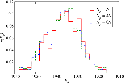
Figure 7: (Color online) Ground-state energy $E_{0}$ histogram showing the fraction of samples at each energy, for the disordered three-spin Ising model on a triangular lattice with $L=36$. Variation among the population sizes shows that the true ground state is not reached in every case, although the centers of the distributions are very close together and shapes of the distribution are similar.

Finally, we estimate the ground-state energy density of the two-dimensional spin glass with $p=3$ on a triangular lattice. The ground-state energy $E_{0}$ [the lowest energy possible in Eq. (2)] is computed for 400 samples for each of $L=12$, $18$, $24$, $30$, $36$, and $42$. Based on the convergence of the ground-state energy histogram, the error is dominated by the statistical fluctuations among samples: Any systematic error in the average is expected to be less than this statistical error. To extrapolate to the thermodynamic limit we plot the energy density at each system size $L$, $E_{0}/L^{2}$ as a function of $1/L$ and take the limit as $1/L\rightarrow 0$, as shown in Fig. 8. Because the system sizes are moderate, finite-size effects can be seen in the data. In order to fairly extrapolate to $L\rightarrow\infty$, we perform linear and quadratic curve fits, varying which system sizes to include in the curve fits. Two example linear curve fits are shown in Fig. 8: The solid line includes $L\geq 24$, whereas the dot-dashed line includes $L\geq 18$. The quadratic fit, which includes all $L$ values shown, gives a similar value for the thermodynamic extrapolation. From these fits, we estimate that the ground-state energy density in the disordered Ising model with $p=3$ on a triangular lattice is $-1.499(3)$.

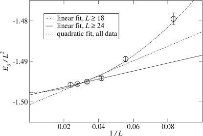
Figure 8: Ground-state energy density, $E_{0}/L^{2}$ of the disordered Ising model with $p=3$ on a triangular lattice. The plaquette interactions are bimodally distributed with positive and negative interactions being equally probable. To extrapolate to the thermodynamic limit, we performed linear and quadratic fits, as shown. Our estimate of the ground-state energy density in this model is $-1.499(3)$.

VI Conclusions

We have shown that the optimization of a disordered Ising model with three-spin interactions is an NP-hard problem in two dimensions, so that efficient exact algorithms are not expected to exist, even for simple cases of glassy $p$-spin models. Optimization of NP-hard problems is a difficult task: We map this problem onto an integer linear program problem and can find exact ground states using a branch-and-cut technique. This works well in small systems, but takes time exponential in the size of the system. To better address physical problems in $p$-spin models, heuristic approaches are important. We present an effective heuristic algorithm that combines a genetic approach with local search optimization to give ground states with high confidence in systems of up to several thousand spins. This algorithm is simple and general: Our implementation can work for any geometry and with any spin interactions. These techniques should prove useful for future work on the low-temperature glassy dynamics of $p$-spin models.