Soliton-like solutions for nonlinear Schrödinger equation with variable quadratic Hamiltonians

Abstract.

We construct one soliton solutions for the nonlinear Schrödinger equation with variable quadratic Hamiltonians in a unified form by taking advantage of a complete (super) integrability of generalized harmonic oscillators. The soliton wave evolution in external fields with variable quadratic potentials is totally determined by the linear problem, like motion of a classical particle with acceleration, and the (self-similar) soliton shape is due to a subtle balance between the linear Hamiltonian (dispersion and potential) and nonlinearity in the Schrödinger equation by the standards of soliton theory. Most linear (hypergeometric, Bessel) and a few nonlinear (Jacobian elliptic, second Painlevé transcendental) classical special functions of mathematical physics are linked together through these solutions, thus providing a variety of nonlinear integrable cases. Examples include bright and dark solitons, and Jacobi elliptic and second Painlevé transcendental solutions for several variable Hamiltonians that are important for current research in nonlinear optics and Bose–Einstein condensation. The Feshbach resonance matter wave soliton management is briefly discussed from this new perspective.

1. Introduction

Advances of the past decades in nonlinear optics, Bose–Einstein condensates, propagation of soliton waves in plasma physics and in other fields of nonlinear science have involved a detailed study of nonlinear Schrödinger equations (see, for example, [9], [17], [81], [149], [151] and references therein). In the theory of Bose–Einstein condensation [42], [114], from a general point of view, the dynamics of gases of cooled atoms in a magnetic trap at very low temperatures can be described by an effective equation for the condensate wave function known as the Gross–Pitaevskii (or nonlinear Schrödinger) equation [16], [69], [70], [76], [108] and [113]. Experimental observations of dark and bright solitons [18], [20], [44], [75] and bright soliton trains [9], [129], [130] in the presence of harmonic confinement have generated considerable research interest in this area [16], [58].

The propagation of an optical pulse in a real fiber is also well described by a nonlinear Schrödinger equation for the envelope of wave functions travelling inside the fiber [4], [7], [17], [46], [61], [77]. A class of self-similar solutions that exists for physically realistic dispersion and nonlinearity profiles in a fiber with anomalous group velocity dispersion is discussed in [78], [79], [97], [98], [116], [123], [125], which suggests, among other things, a method of pulse compression and a model of steady-state asynchronous laser mode locking [98]. Solutions of a nonhomogeneous Schrödinger equation are also known for propagation of soliton waves in plasma physics [13], [22], [23], [104].

Integration techniques of the nonlinear Schrödinger equation include Painlevé analysis [10], [17], [30], [31], [32], [33], [63], [81], [102], [144], Hirota method [64], [65], [81], Lax method [10], [81], [84], [151], Miura transformation [94], [95], inverse scattering transform and Hamiltonian approach [2], [3], [6], [55], [59], [105] among others [21], [45], [51], [89], [107], [120]. Although the classical soliton concept was developed for nonlinear autonomous dispersive systems with time being an independent variable only, not appearing in the nonlinear evolution equations (see [126], [127] for highlighting this point), connections between autonomous and nonautonomous Schrödinger equations have been discussed in [2], [4], [27], [62], [82], [98], [112], [116] and [155] (see Remark 2 for an explicit transformation). The formation of matter wave solitons in Bose–Einstein condensation by magnetically tuning the interatomic interaction near the Feshbach resonance provides an example of nonautonomous systems that are currently under investigation [16], [58], [130].

We elaborate on results of recent papers [9], [10], [12], [17], [52], [85], [24], [62], [63], [78], [79], [82], [80], [118], [123], [124], [125], [126], [127], [129], [140], [146], [147], [148], [149] on construction of exact solutions of the nonlinear Schrödinger equation with variable quadratic Hamiltonians (see also [136] and [151], [152], [153]). In this paper, a unified form of these soliton-like (self-similar) solutions is presented, thus combining progress of the soliton theory with a complete integrability of generalized harmonic oscillators. We show, in general, that the soliton evolution in external fields described by variable quadratic potentials is totally determined by the linear problem, similar to the motion of a classical particle with acceleration, while the original soliton shape is due to a delicate balance between the linear Hamiltonian (dispersion and potential) and nonlinearity in the Schrödinger equation according to basic principles of the soliton theory. Examples include bright and dark solitons, and Jacobi elliptic and Painlevé II transcendental solutions for solitary wave profiles, which are important in nonlinear optics [4], [22], [23], [78], [79], [97], [123], [125], [151] and Bose–Einstein condensation [12], [9], [127], [129], [148].

The paper is organized as follows. We present a unified form of one soliton solutions with integrability conditions, and sketch the proof in the next two sections, respectively. In Section 4, more details are provided and some simple examples are discussed. Section 5 deals with a Feshbach resonance management of matter wave solitons. In the last section, an extension of our method is given and a classical example of accelerating soliton in a linearly inhomogeneous plasma [22], [23] is revisited from a new perspective. An attempt to collect most relevant bibliography is made but in view of a rich history and the very high publication rate in these research areas we must apologize in advance if some important papers are missing.

2. Soliton-Like Solutions

The nonlinear Schrödinger equation

$$i\frac{\partial\psi}{\partial t}=H\psi+g\psi+h\left|\psi\right|^{2}\psi,$$ (2.1)

where the variable Hamiltonian $H$ is a quadratic form of operators $p=-i\partial/\partial x$ and $x,$ namely,

$$i\psi_{t}=-a\left(t\right)\psi_{xx}+b\left(t\right)x^{2}\psi-ic\left(t\right)x\psi_{x}-id\left(t\right)\psi+g\left(x,t\right)\psi+h\left(t\right)\left|\psi\right|^{2}\psi$$ (2.2)

($a,$ $b,$ $c,$ $d$ are suitable real-valued functions of time only) has the following soliton-like solutions

$$\psi\left(x,t\right) = \frac{e^{i\phi}}{\sqrt{\mu\left(t\right)}}\exp\left(i\left(\alpha\left(t\right)x^{2}+\beta\left(t\right)xy+\gamma\left(t\right)y^{2}\right)\right)$$

$$\times F\left(\beta\left(t\right)x+2\gamma\left(t\right)y\right)$$

($\phi$ is a real constant, $y$ is a parameter and $\mu,$ $\alpha,$ $\beta,$ $\gamma$ are real-valued functions of time only given by equations (2.16)–(2.22) below), provided that

$$g=g_{0}a\left(t\right)\beta^{2}\left(t\right)\left(\beta\left(t\right)x+2\gamma\left(t\right)y\right)^{m},\qquad h=h_{0}a\left(t\right)\beta^{2}\left(t\right)\mu\left(t\right)$$ (2.4)

($g_{0}$ and $h_{0}$ are constants and $m=0,1).$ As we shall see in the next section, these (integrability) conditions control the balance between the linear Hamiltonian (dispersion and potential) and nonlinearity in the Schrödinger equation (2.2) thus making possible an existence of the soliton-like solution (with damping or amplification) in the presence of variable quadratic potentials (see also [12], [63], [126], [127] and [154] for discussion of important special cases; Remark 2 provides an important interpretation of relations (2.4) as a complete integrability condition for the nonautonomous nonlinear Schrödinger equation (2.1) when $m=0).$

Here, the soliton profile function $F\left(z\right)$ of a single travelling wave-type argument $z=$ $\beta x+2\gamma y$ satisfies the ordinary nonlinear differential equation of the form

$$F^{\prime\prime}\left(z\right)=g_{0}z^{m}F\left(z\right)+h_{0}F^{3}\left(z\right).$$ (2.5)

If $m=0,$ with the help of an integrating factor,

$$\left(\frac{dF}{dz}\right)^{2}=C_{0}+g_{0}F^{2}+\frac{1}{2}h_{0}F^{4}\qquad\left(C_{0}\text{ is a constant}\right),$$ (2.6)

which can be solved in terms of Jacobian elliptic functions [8], [53], [81], [143]. When $m=1,$ equation (2.5) leads to Painlevé II transcendents [6], [28], [31], [33], [81].

The variable phase is given in terms of solutions of the following system of ordinary differential equations:

$$\frac{d\alpha}{dt}+b+2c\alpha+4a\alpha^{2}=0,$$ (2.7)

$$\frac{d\beta}{dt}+\left(c+4a\alpha\right)\beta=0,$$ (2.8)

$$\frac{d\gamma}{dt}+a\beta^{2}=0$$ (2.9)

(see Ref. [34] and the next section for more details), where the standard substitution

$$\alpha=\frac{1}{4a\left(t\right)}\frac{\mu^{\prime}\left(t\right)}{\mu\left(t\right)}-\frac{d\left(t\right)}{2a\left(t\right)}$$ (2.10)

reduces the Riccati equation (2.7) to the second order linear equation

$$\mu^{\prime\prime}-\tau\left(t\right)\mu^{\prime}+4\sigma\left(t\right)\mu=0$$ (2.11)

with

$$\tau\left(t\right)=\frac{a^{\prime}}{a}-2c+4d,\qquad\sigma\left(t\right)=ab-cd+d^{2}+\frac{d}{2}\left(\frac{a^{\prime}}{a}-\frac{d^{\prime}}{d}\right).$$ (2.12)

(Relations with the corresponding Ehrenfest theorem for the linear Hamiltonian are discussed in Ref. [36].)

It is worth noting that in the soliton-like solution under consideration (2) linear and nonlinear factors are essentially separated, namely, the nonlinear part is represented only by the profile function $F$ of a single travelling wave variable $z=\beta x+2\gamma y$ as solution of the nonlinear equation (2.5). Letting $\beta x+2\gamma y=$constant, one obtains

$$x^{\prime}+\frac{\beta^{\prime}}{\beta}x=2a\beta y$$ (2.13)

and

$$x^{\prime\prime}-\frac{a^{\prime}}{a}x^{\prime}+\left(\left(\frac{\beta^{\prime}}{\beta}\right)^{\prime}-\frac{a^{\prime}}{a}\frac{\beta^{\prime}}{\beta}-\left(\frac{\beta^{\prime}}{\beta}\right)^{2}\right)x=0$$ (2.14)

for the soliton velocity and acceleration with the aid of (2.9). Then, by (2.7)–(2.8):

$$x^{\prime\prime}-\frac{a^{\prime}}{a}x^{\prime}+\left(4ab-c^{2}+c\left(\frac{a^{\prime}}{a}-\frac{c^{\prime}}{c}\right)\right)x=0$$ (2.15)

that is similar to equation of motion of a classical particle (damped parametric oscillations).

The initial value problem for the system (2.7)–(2.9), which corresponds to the linear Schrödinger equation with a variable quadratic Hamiltonian (generalized harmonic oscillators [15], [49], [60], [145], [150]), can be explicitly solved in terms of solutions of our characteristic equation (2.11) as follows [34], [36], [132], [133]:

$$\mu\left(t\right)=2\mu\left(0\right)\mu_{0}\left(t\right)\left(\alpha\left(0\right)+\gamma_{0}\left(t\right)\right),$$ (2.16)

$$\alpha\left(t\right)=\alpha_{0}\left(t\right)-\frac{\beta_{0}^{2}\left(t\right)}{4\left(\alpha\left(0\right)+\gamma_{0}\left(t\right)\right)},$$ (2.17)

$$\beta\left(t\right)=-\frac{\beta\left(0\right)\beta_{0}\left(t\right)}{2\left(\alpha\left(0\right)+\gamma_{0}\left(t\right)\right)}=\frac{\beta\left(0\right)\mu\left(0\right)}{\mu\left(t\right)}\lambda\left(t\right),$$ (2.18)

$$\gamma\left(t\right)=\gamma\left(0\right)-\frac{\beta^{2}\left(0\right)}{4\left(\alpha\left(0\right)+\gamma_{0}\left(t\right)\right)},$$ (2.19)

where

$$\alpha_{0}\left(t\right)=\frac{1}{4a\left(t\right)}\frac{\mu_{0}^{\prime}\left(t\right)}{\mu_{0}\left(t\right)}-\frac{d\left(t\right)}{2a\left(t\right)},$$ (2.20)

$$\beta_{0}\left(t\right)=-\frac{\lambda\left(t\right)}{\mu_{0}\left(t\right)},\qquad\lambda\left(t\right)=\exp\left(-\int_{0}^{t}\left(c\left(s\right)-2d\left(s\right)\right)\ ds\right),$$ (2.21)

$$\gamma_{0}\left(t\right)=\frac{1}{2\mu_{1}\left(0\right)}\frac{\mu_{1}\left(t\right)}{\mu_{0}\left(t\right)}+\frac{d\left(0\right)}{2a\left(0\right)}$$ (2.22)

provided that $\mu_{0}$ and $\mu_{1}$ are the standard solutions of equation (2.11) corresponding to the following initial conditions $\mu_{0}\left(0\right)=0,$ $\mu_{0}^{\prime}\left(0\right)=2a\left(0\right)\neq 0$ and $\mu_{1}\left(0\right)\neq 0,$ $\mu_{1}^{\prime}\left(0\right)=0.$ (Formulas (2.20)–(2.22) correspond to Green’s function of generalized harmonic oscillators; see, for example, [34], [36], [50], [88], [132], [133] and references therein for more details.)

The continuity with respect to initial data,

$$\lim_{t\rightarrow 0^{+}}\alpha\left(t\right)=\alpha\left(0\right),\quad\lim_{t\rightarrow 0^{+}}\beta\left(t\right)=\beta\left(0\right),\quad\lim_{t\rightarrow 0^{+}}\gamma\left(t\right)=\gamma\left(0\right),$$ (2.23)

has been established in [132] for suitable smooth coefficients of the linear Schrödinger equation. Thus the soliton-like solution (2) evolves to the future $t>0$ starting from the following initial data:

$$\psi\left(x,0\right) = \lim_{t\rightarrow 0^{+}}\psi\left(x,t\right)$$

$$= \frac{e^{i\phi}}{\sqrt{\mu\left(0\right)}}\exp\left(i\left(\alpha\left(0\right)x^{2}+\beta\left(0\right)xy+\gamma\left(0\right)y^{2}\right)\right)$$

$$\times F\left(\beta\left(0\right)x+2\gamma\left(0\right)y\right),$$

where $\phi,$ $\mu\left(0\right),$ $\alpha\left(0\right),$ $\beta\left(0\right),$ $\gamma\left(0\right)$ and $y$ are arbitrary real parameters (see also (6) for a more general solution of this form).

Remark 1.

When $m=0,$ the gauge transformation $\psi=\chi\left(x,t\right)\exp\left[ig_{0}\left(\gamma\left(t\right)-\gamma\left(0\right)\right)\right]$ changes the original equation (2.2) into

$$i\chi_{t}=-a\left(t\right)\chi_{xx}+b\left(t\right)x^{2}\chi-ic\left(t\right)x\chi_{x}-id\left(t\right)\chi+h\left(t\right)\left|\chi\right|^{2}\chi,$$ (2.25)

where $a,$ $b,$ $c,$ $d$ are suitable real-valued functions of time $t$ only and

$$h\left(t\right)=h_{0}\beta^{2}\left(0\right)\mu^{2}\left(0\right)\frac{a\left(t\right)\lambda^{2}\left(t\right)}{\mu\left(t\right)},$$ (2.26)

which is more common in practice. Once again, classical solution of the linear equation (2.11), namely, our characteristic function $\mu\left(t\right),$ completely controls the specific form of the nonlinearity factor $h\left(t\right)$ required for creation of the soliton (an extension is given in Section 6; see also Refs. [12], [126] and [127] for important special cases).

Remark 2.

A simple change of variables,

$$\psi=\frac{1}{\sqrt{\mu}}e^{i\alpha x^{2}}\chi\left(\beta x,\gamma\right),$$ (2.27)

transforms the nonautonomous equation (2.2) with conditions (2.4), when $m=0,$ into a standard autonomous nonlinear Schrödinger equation with respect to the new variables $\xi=\beta x$ and $\tau=\gamma:$

$$i\chi_{t}+g_{0}\chi+h_{0}\left|\chi\right|^{2}\chi=\chi_{\xi\xi},$$ (2.28)

which is completely integrable by advanced methods of the soliton theory [2], [6], [81], [151] (see also [45] and references cited in the introduction). This observation provides an alternative approach to derivation of our equations (2.7)–(2.10). An extension of the transformation (2.27) is given in [134].

3. Sketch of the Proof

Following [34] (see also [22], [91] and [118]), we are looking for exact solutions of the form

$$\psi=A\left(x,t\right)e^{iS\left(x,t\right)},\quad S\left(x,t\right)=\alpha\left(t\right)x^{2}+\beta\left(t\right)xy+\gamma\left(t\right)y^{2}$$ (3.1)

($y$ is a parameter). Substituting into (2.2) and taking the imaginary part,

$$A_{t}+\left(\left(4a\alpha+c\right)x+2a\beta y\right)A_{x}+\left(2\alpha a+d\right)A=0.$$ (3.2)

For the real part, equating coefficients of all admissible powers of $x^{m}y^{n}$ with $m+n=2,$ one gets our system of ordinary differential equations (2.7)–(2.9) of the corresponding linear Schrödinger equation with the unique solution (2.16)–(2.22) already obtained in Refs. [34], [132], [133] and/or elsewhere. In addition, an auxiliary nonlinear equation of the form

$$aA_{xx}=gA+hA^{3}$$ (3.3)

appears as a contribution from the last two terms. With the help of (2.8) and (2.10) our equation (3.2) can be rewritten as

$$A_{t}-\left(\frac{\beta^{\prime}}{\beta}x-2a\beta y\right)A_{x}+\frac{1}{2}\frac{\mu^{\prime}}{\mu}A=0.$$ (3.4)

Looking for a travelling wave solution with damping or amplification:

$$A=A\left(x,t\right)=\frac{1}{\sqrt{\mu\left(t\right)}}\ F\left(z\right),\qquad z=c_{0}\left(t\right)x+c_{1}\left(t\right)y,$$ (3.5)

one gets

$$c_{0}^{\prime}x+c_{1}^{\prime}y=\left(\frac{\beta^{\prime}}{\beta}x-2a\beta y\right)c_{0}$$ (3.6)

with $c_{0}=\beta$ and $c_{1}=2\gamma$ (or $z=\beta x+2\gamma y).$ Then equation (3.3) takes the form

$$\frac{d^{2}}{dz^{2}}F\left(z\right)=\frac{g}{a\beta^{2}}F\left(z\right)+\frac{h}{a\beta^{2}\mu}F^{3}\left(z\right),$$ (3.7)

which must have all coefficients depending on $z$ only in order to preserve a self-similar profile of the travelling wave with damping or amplification. This results in the required equation (2.5) under the balancing conditions (2.4) and our proof is complete. (An extension is given in Section 6.)

Remark 3.

Assuming in (3.4) that

$$A\left(x,t\right)=\frac{1}{\sqrt{\mu\left(t\right)}}\ B\left(\xi,\tau\right),$$ (3.8)

where $\xi=\beta x$ and $\tau=2\gamma y,$ implies $B_{\xi}=B_{\tau}$ with a general solution $B\left(\xi,\tau\right)=F\left(\xi+\tau\right)=F\left(\beta x+2\gamma y\right).$

4. Details and Examples

A brief description of the method under consideration is as follows. In order to obtain soliton-like solutions (2) explicitly, say in terms of elementary and/or transcendental functions, one has to solve, in general, the nonlinear equation (2.5) for the profile function $F\left(z\right)$ in terms of Jacobian elliptic functions [8], [53], [81], [115], [143] (some elementary solutions are also available), when $m=0,$ or in terms of Painlevé II transcendents, when $m=1$ (it is known that if $m>1,$ this equation does not have the Painlevé property [6], [81]). In addition, one has to solve the linear characteristic equation (2.11), which has a variety of solutions in terms of elementary and special (hypergeometric, Bessel) functions [11], [87], [103], [115], [142]. Many elementary solutions of the corresponding linear Schrödinger equation for generalized harmonic oscillators are known explicitly (see, for example, [34], [35], [36], [37], [50], [88], [133], [145], [150] and references therein). Then, the linear part allows determination of the travelling wave argument $z=\beta x+2\gamma y$ and the damping (or amplifying) factor $\mu^{-1/2}$ of the soliton-like solution (2). Our balancing conditions (2.4) control dispersion, potential and nonlinearity in the original nonlinear Schrödinger equation (2.2), which is crucial for the soliton existence. (An extension is discussed in Section 6.)

4.1. Nonlinear Part

When $m=0,$ equation (2.5) is integrated to the first order equation (2.6) and (the corresponding initial value problem) can be solved by the reduction of elliptic integrals in terms of Jacobian or Weierstrass (doubly) periodic elliptic functions [8], [53], [79], [81]. We are interested in real-valued solutions. Some of the classical nonlinear wave configurations are given by

$$F\left(z\right) = \left(\frac{g_{0}+\sqrt{g_{0}^{2}-2C_{0}h_{0}}}{-h_{0}}\right)^{1/2}$$

$$\times\text{cn}\left(\left(g_{0}^{2}-2C_{0}h_{0}\right)^{1/4}z,\left(\frac{g_{0}+\sqrt{g_{0}^{2}-2C_{0}h_{0}}}{2\sqrt{g_{0}^{2}-2C_{0}h_{0}}}\right)^{1/2}\right),$$

if $h_{0}<0$ and

$$F\left(z\right) = \left(\frac{-g_{0}+\sqrt{g_{0}^{2}-2C_{0}h_{0}}}{h_{0}}\right)^{1/2}$$

$$\times\text{sn}\left(\left(\frac{C_{0}h_{0}}{-g_{0}+\sqrt{g_{0}^{2}-2C_{0}h_{0}}}\right)z,\left(\frac{g_{0}-\sqrt{g_{0}^{2}-2C_{0}h_{0}}}{g_{0}+\sqrt{g_{0}^{2}-2C_{0}h_{0}}}\right)^{1/2}\right),$$

if $g_{0}<0.$ Here, cn$\left(u,k\right)$ and sn$\left(u,k\right)$ are the Jacobi elliptic functions [8], [53], [143]. Familiar special cases include the bright soliton:

$$F\left(z\right)=\sqrt{\frac{2g_{0}}{-h_{0}}}\frac{1}{\cosh\left(\sqrt{g_{0}}z\right)}$$ (4.3)

with $C_{0}=0$ in (4.1) and the dark soliton:

$$F\left(z\right)=\sqrt{\frac{-g_{0}}{h_{0}}}\tanh\left(\sqrt{\frac{-g_{0}}{2}}z\right)$$ (4.4)

with $C_{0}=g_{0}^{2}/\left(2h_{0}\right)$ in (4.1), when cn$\left(u,1\right)=1/\cosh u$ and sn$\left(u,1\right)=\tanh u,$ respectively (the real period tends to infinity). More details can be found in Refs. [8], [53], [57], [79], [143], [151] and/or elsewhere.

If $m=1,$ the substitution $F\left(z\right)=g_{0}^{1/3}\sqrt{2/h_{0}}\ w\left(\zeta\right)$ and $\zeta=zg_{0}^{1/3}$ transforms (2.5) into the second Painlevé equation,

$$w^{\prime\prime}=\zeta w+2w^{3}.$$ (4.5)

In the limit $w\rightarrow 0,$ this equation reduces to the Airy equation and its solution may be thought of as a nonlinear generalization of an Airy function [5]. There is a one-parameter family of real solutions $w=A_{k}\left(\zeta\right)$ that are bounded for all real $\zeta$ with the following asymptotic properties:

$$A_{k}\left(\zeta\right)=\left\{\begin{array}[]{c}k\text{Ai\/}\left(\zeta\right),\qquad\zeta\rightarrow+\infty\vskip 12.0pt plus 4.0pt minus 4.0pt\\ r\left|\zeta\right|^{-1/4}\sin\left(s\left(\zeta\right)-\theta_{0}\right)+\text{o}\left(\left|\zeta\right|^{-1/4}\right),\quad\zeta\rightarrow-\infty\vskip 12.0pt plus 4.0pt minus 4.0pt\end{array}\right.$$ (4.6)

Here, Ai$\left(\zeta\right)$ is the Airy function, $-1<k<1$ provided $k\neq 0,$ $r^{2}=-\pi^{-1}\ln\left(1-k^{2}\right),$

$$s\left(\zeta\right)=\frac{2}{3}\left|\zeta\right|^{3/2}-\frac{3}{4}r^{2}\ln\left|\zeta\right|$$ (4.7)

and

$$\theta_{0}=\frac{3}{2}r^{2}\ln 2+\arg\Gamma\left(1-\frac{i}{2}r^{2}\right)+\frac{\pi}{4}\left(1-2\text{sign\/}\left(k\right)\right).$$ (4.8)

These asymptotics were found in [5], [122] and, eventually, had been proven rigorously in [47], [48] (see [6], [14], [28], [29], [31], [33], [135] and references therein for study of this nonlinear Airy function; graphs of these functions are presented in [28], see Figure 1 for an example: $w_{.5}=A_{1/2}\left(x\right).)$ An application to a soliton moving with a constant velocity in linearly inhomogeneous plasma is discussed in Section 6.

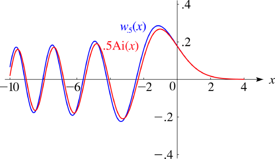
Figure 1. Graphs of the Airy function $.5$Ai$\left(x\right)$ and the nonlinear Airy function $w_{.5}=A_{1/2}\left(x\right)$ (red and blue in an electronic version, respectively, [28]).

4.2. Linear Part

Generalized harmonic oscillators [15], [49], [60], [145], [150], which correspond to the Schrödinger equation with variable quadratic Hamiltonians, are well studied in quantum mechanics (see also [34], [35], [50], [83], [88], [133] and references therein for a general approach and known elementary and transcendental solutions). A few examples include the Caldirola–Kanai Hamiltonian of the quantum damped oscillator [19], [43], [72], [141] and some of its natural modifications; a modified oscillator considered by Meiler, Cordero-Soto and Suslov [92], [37], and the degenerate parametric oscillator [38]; the quantum damped oscillator of Chruściński and Jurkowski [26], and a quantum-modified parametric oscillator among others. Green’s functions are derived in a united way in Ref. [36].

4.3. Examples

Combination of linear and nonlinear parts by our formula (2) results in numerous explicit soliton-like solutions for corresponding nonlinear Schrödinger equations. It is worth noting that in this approach most linear and some nonlinear classical special functions of mathematical physics are linked together through these solutions.

4.3.1. Nonlinear Optics

In the simplest form,

$$i\frac{\partial\psi}{\partial t}=\frac{\partial^{2}\psi}{\partial x^{2}}+g\psi+h\left|\psi\right|^{2}\psi,$$ (4.9)

one gets [34], [97], [98]

$$\alpha\left(t\right)=\frac{\alpha_{0}}{1-4\alpha_{0}t},\qquad\qquad\beta\left(t\right)=\frac{\beta_{0}}{1-4\alpha_{0}t},$$ (4.10)

$$\gamma\left(t\right)=\gamma_{0}+\frac{\beta_{0}^{2}t}{1-4\alpha_{0}t},\quad\mu\left(t\right)=\mu_{0}\left(1-4\alpha_{0}t\right)$$

($\mu_{0},$ $\alpha_{0},$ $\beta_{0},$ $\gamma_{0}$ are constants) and

$$z=\frac{\beta_{0}x+2\left(\gamma_{0}+\left(\beta_{0}^{2}-4\alpha_{0}\gamma_{0}\right)t\right)y}{1-4\alpha_{0}t},$$ (4.11)

$$g\left(x,t\right)=-\frac{g_{0}\beta_{0}^{2}}{\left(1-4\alpha_{0}t\right)^{2}}z^{m}\qquad\left(m=0,1\right),$$ (4.12)

$$h\left(t\right)=-\frac{h_{0}\mu_{0}\beta_{0}^{2}}{1-4\alpha_{0}t}.$$ (4.13)

(Traditionally, $\alpha_{0}=0$ and $m=0$ with $\psi=\chi\exp\left(ig_{0}\beta_{0}^{2}t\right)$ [81], [151]. The case $m=1$ is discussed in Section 6.)

The case $b=c=0,$

$$i\psi_{t}=-a\psi_{xx}-id\psi+g\psi+h\left|\psi\right|^{2}\psi,$$ (4.14)

is of interest in fiber optics (see, for example, [4], [7], [61], [77], [78], [79], [97], [98], [116], [119], [123], [124], [126], [127] and references therein). Here, all parameters $a\left(t\right),$ $d\left(t\right)$ and $h\left(t\right)$ are functions of the propagation distance $t=z$ and this equation describes the amplification or attenuation (if $d$ is positive) of pulses propagating nonlinearly in a single-mode optical fiber, where $\psi\left(t,x\right)$ is the complex envelope of the electrical field in a comoving frame, $x=\tau$ is the retarded time, $a\left(t\right)$ is the group velocity dispersion parameter, $d\left(t\right)$ is the dispersion gain or loss function, and $h\left(t\right)$ is the nonlinearity parameter [78], [79].

The substitution $\psi=\chi e^{-\Lambda},$ $\Lambda\left(t\right)=\int_{0}^{t}d\left(s\right)\ ds$ results in

$$i\frac{\partial\chi}{\partial t}=-a\frac{\partial^{2}\chi}{\partial x^{2}}+g\chi+he^{-2\Lambda}\left|\chi\right|^{2}\chi,$$ (4.15)

which, of course, can be solved by the method under consideration, but a standard change of the time variable,

$$\tau=-\int_{0}^{t}a\left(s\right)\ ds,$$ (4.16)

transforms this equation into the previous one. Just replace $t\rightarrow\tau$ (see also [78], [79], [123], [124] and [125], where this simple observation has been omitted). More general transformations are discussed in Refs. [2], [27], [35], [82], [98], [112], [116], [134], [155].

4.3.2. Harmonic Solitons

In a similar fashion, one can show that the nonlinear Schrödinger equation of the form

$$i\frac{\partial\chi}{\partial t}=\frac{1}{2}\left(-\frac{\partial^{2}\chi}{\partial x^{2}}+x^{2}\chi\right)+\frac{h_{0}\mu_{0}\beta_{0}^{2}}{2\left(\cos t+2\alpha_{0}\sin t\right)}\left|\chi\right|^{2}\chi$$ (4.17)

has the following explicit solution:

$$\chi\left(x,t\right)=\frac{e^{iS\left(x,t\right)}}{\sqrt{\left|\mu_{0}\right|\left(\cos t+2\alpha_{0}\sin t\right)}}\ F\left(z\right),$$ (4.18)

where

$$z=\frac{\beta_{0}x+\left(2\gamma_{0}\cos t-\left(\beta_{0}^{2}-4\alpha_{0}\gamma_{0}\right)\sin t\right)y}{\cos t+2\alpha_{0}\sin t}$$ (4.19)

and

$$S\left(x,t\right) = \frac{2\alpha_{0}\cos t-\sin t}{2\left(\cos t+2\alpha_{0}\sin t\right)}x^{2}+\frac{\beta_{0}xy}{\cos t+2\alpha_{0}\sin t}$$

$$+\frac{2\gamma_{0}\cos t-\left(\beta_{0}^{2}-4\alpha_{0}\gamma_{0}\right)\sin t}{2\left(\cos t+2\alpha_{0}\sin t\right)}y^{2}+\frac{g_{0}\beta_{0}^{2}\sin t}{2\left(\cos t+2\alpha_{0}\sin t\right)}$$

provided

$$F^{\prime\prime}=g_{0}F+h_{0}F^{3}$$ (4.21)

($m=0,$ $\mu_{0}\neq 0,$ $\alpha_{0},$ $\beta_{0},$ $\gamma_{0},$ $g_{0},$ $h_{0}$ and $y$ are arbitrary real constants). The reader may choose the profile function $F,$ say in one of the forms (4.1)–(4.4).

If $m=1,$ the Schrödinger equation,

$$i\frac{\partial\psi}{\partial t} = \frac{1}{2}\left(-\frac{\partial^{2}\psi}{\partial x^{2}}+x^{2}\psi\right)+\frac{g_{0}\beta_{0}^{2}}{2\left(\cos t+2\alpha_{0}\sin t\right)^{2}}z\psi$$

$$+\frac{h_{0}\mu_{0}\beta_{0}^{2}}{2\left(\cos t+2\alpha_{0}\sin t\right)}\left|\psi\right|^{2}\psi,$$

has a solution-like solution of the form (4.18) (last term in (4.3.2) should be omitted) provided that

$$F^{\prime\prime}=g_{0}zF+h_{0}F^{3},$$ (4.23)

which solution is given in terms of the nonlinear Airy function $A_{k}\left(\zeta\right).$ Further details are left to the reader (see also Section 6).

5. Matter Wave Solitons

5.1. Gross–Pitaevskii equation

Discovery of Bose–Einstein condensates in ultra-cold gases of weakly interacting alkali-metal atoms has stimulated intensive studies of nonlinear matter waves on a macroscopic scale (see, for example, [16], [39], [58], [73], [130]). The Gross–Pitaevskii equation for a zero-temperature condensate of atoms, confined in a cylindrical trap $V_{0}\left(x,y\right)=m\omega_{\bot}^{2}\left(x^{2}+y^{2}\right)/2,$ and a time-dependent harmonic confinement, which can be either attractive or expulsive, along the $z$ direction, $V_{1}\left(z,t\right)=m\omega_{0}^{2}\left(t\right)z^{2}/2,$ is given by [12], [42], [54], [86], [114], [121], [127]:

$$i\hslash\frac{\partial\Psi\left(\boldsymbol{r},t\right)}{\partial t}=\left(-\frac{\hslash^{2}}{2m}\Delta+V_{\text{ext}}\left(\boldsymbol{r},t\right)+U\left|\Psi\left(\boldsymbol{r},t\right)\right|^{2}+i\frac{\hslash\eta\left(t\right)}{2}\right)\Psi\left(\boldsymbol{r},t\right),$$ (5.1)

where $U=4\pi\hslash^{2}a_{s}/m,$ $a_{s}$ is the $s$-wave scattering length, $m$ is the mass of the atom, $V_{\text{ext}}=V_{0}\left(x,y\right)+V_{1}\left(z,t\right)$ and the condensate interaction with the normal atomic cloud through three-body interaction is phenomenologically incorporated by a gain or loss term $\eta\left(t\right).$ If the interaction energy of atoms is much less that the kinetic energy in the transverse direction, then the substitution

$$\Psi\left(\boldsymbol{r},t\right)=\frac{1}{\sqrt{2\pi a_{0}}a_{\bot}}\exp\left(-i\omega_{\bot}t-\frac{x^{2}+y^{2}}{2a_{\bot}^{2}}+\frac{\Lambda\left(t\right)}{2}\right)$$ (5.2)

$$\quad\qquad\quad\times\psi\left(\frac{z}{a_{\bot}},\omega_{\bot}t\right),\qquad\qquad\Lambda\left(t\right)=\int_{0}^{t}\eta\left(s\right)\ ds$$

allows one to reduce the three-dimensional Gross–Pitaevskii equation (5.1) to the following one-dimensional nonlinear Schrödinger equation in new dimensionless units $\zeta=z/a_{\bot}$ and $\tau=\omega_{\bot}t:$

$$i\frac{\partial\psi}{\partial\tau}=\frac{1}{2}\left(-\frac{\partial^{2}\psi}{\partial\zeta^{2}}+\omega^{2}\left(\tau\right)\zeta^{2}\psi\right)+\kappa\left(\tau\right)\left|\psi\right|^{2}\psi.$$ (5.3)

Here,

$$\kappa\left(\tau\right)=2e^{\Lambda}\frac{a_{s}}{a_{0}},\qquad\omega^{2}\left(\tau\right)=\frac{\omega_{0}^{2}}{\omega_{\bot}^{2}},\qquad a_{\bot}=\sqrt{\frac{\hslash}{m\omega_{\bot}}}$$ (5.4)

and $a_{0}$ is the Bohr radius (see Refs. [68], [76], [93], [99], [100], [111], [121] for more details).

Letting

$$\psi=\chi\exp\left(i\int_{0}^{\tau}g\left(s\right)\ ds\right)$$ (5.5)

with the function $g\left(\tau\right)$ given by (5.9) below, equation (5.3) can be transformed into (2.2), where

$$a=\frac{1}{2},\quad b=\frac{1}{2}\omega^{2}\left(\tau\right),\quad c=d=0,\quad h=\kappa\left(\tau\right).$$ (5.6)

Then our characteristic equation (2.11) take the form

$$\mu^{\prime\prime}+\omega^{2}\left(\tau\right)\mu=0,$$ (5.7)

which describes the motion of a classical oscillator with variable frequency [87]. (This equation coincides also with the Ehrenfest theorem for the corresponding linear Hamiltonian [36].) Choosing the standard solutions $\mu_{0}\left(\tau\right)$ and $\mu_{1}\left(\tau\right)$ with $\mu_{0}\left(0\right)=0,$ $\mu_{0}^{\prime}\left(0\right)=1$ and $\mu_{1}\left(0\right)\neq 0,$ $\mu_{1}^{\prime}\left(0\right)=0,$ one can use formulas (2.16)–(2.22) with $c=d=0$ in order to solve the linear problem in quadratures. This gives the soliton travelling wave variable $z=\beta x+2\gamma y$ and the following balancing conditions:

$$\kappa\left(\tau\right)=h_{0}\frac{\beta^{2}\left(0\right)\mu^{2}\left(0\right)}{2\mu\left(\tau\right)},$$ (5.8)

$$g\left(\tau\right)=g_{0}\frac{\beta^{2}\left(0\right)\mu^{2}\left(0\right)}{2\mu^{2}\left(\tau\right)},\qquad\int_{0}^{\tau}g\left(s\right)\ ds=g_{0}\left(\gamma\left(0\right)-\gamma\left(\tau\right)\right)$$ (5.9)

when $m=0.$

5.2. Feshbach Resonance

The properties of Bose–Einstein condensed gases can be strongly altered by tuning the external magnetic field. A Feshbach resonance management for Bose–Einstein condensates has been discussed from experimental and theoretical perspectives by many authors (see, for example, [1], [25], [41], [40], [39], [56], [63], [66], [67], [71], [74], [85], [90], [96], [109], [110], [114], [117], [127], [128], [130], [131], [138], [139], [154] and references therein). The Feshbach resonance is a scattering resonance in which pairs of free atoms are tuned via Zeeman effect into resonance with vibrational state of the diatomic molecule [39], [130], [139]. (They are known as Feshbach resonance because of their similarity to scattering resonances described by Herman Feshbach in nuclear collisions.) The strength of the nonlinearity $U$ is defined in terms of $s$-wave scattering length $a_{s},$ namely,

$$U=\frac{4\pi\hslash^{2}a_{s}}{m},$$ (5.10)

and dependence of atomic collision cross section due to existence of the metastable state [39], [56], [71], [128] enables $a_{s}$ to be continuously tuned from positive to negative values. (The scattering length also determines the formation rate, the spectrum of collective excitations, the evolution of the condensate phase, the coupling with the noncondensed atoms, and other important properties [40], [114].) As follows from the experiments, the $s$-wave scattering length is the following function of the applied magnetic field [96]:

$$\frac{a_{s}\left(B\right)}{a_{0}}=a_{\infty}\left(1+\frac{\Delta_{0}}{B_{0}-B}\right)$$ (5.11)

(The Feshbach resonance provides, so to speak, a continuous knob to adjust the atom-atom interaction from repulsive to attractive, and from weak to strong [130]. Thus it is possible to study strongly interacting, weakly or noninteracting, or collapsing condensates [71], all with the same alkali species and experimental setup. When the nonlinearity $U=0,$ one deals with linear modes of a macroscopic harmonic oscillator [76]; see, for example, [83], [50], [88] and references therein for a detailed treatment of the corresponding quantum oscillator with variable frequency.) In the empirically established expression (5.11), $B_{0}$ is the resonant value of the magnetic field, $a_{\infty}$ is the off-resonance scattering length and parameter $\Delta_{0}$ represents the resonance width in units of the Bohr radius $a_{0}$ (see [39], [96], [127], [138], [139] and references therein for more details). Feshbach resonances have been observed in ${}^{85}Rb$ at $164~{}G$ [41], [117], [40], in ${}^{23}Na$ at $853$ and $907~{}G$ [67] and have also been identified in ${}^{6}Li$ [66], [106], [129], [130].

5.3. Matter Wave Soliton Management

The Feshbach resonance provides an effective practical tool for experimental study of the matter wave solitons. Indeed, for creation of a certain soliton configuration one needs to satisfy the following condition:

$$h_{0}\frac{\beta^{2}\left(0\right)\mu^{2}\left(0\right)}{4\mu}e^{-\Lambda}=a_{\infty}\left(1+\frac{\Delta_{0}}{B_{0}-B}\right)$$ (5.12)

in order to synchronize the Feshbach resonance and harmonic trap. (Here, both sides have the same simple pole structure, which can be used in experimental setting.) This equation allows determination of the classical law of motion (kinematics in $z$ direction) of the expectation value $\mu=\langle\Psi,\boldsymbol{r}\Psi\rangle$ with respect to the linear part of Gross–Pitaevskii Hamiltonian (5.1), when $U=\eta=0,$ in terms of  a suitable applied magnetic field $B$ near the Feshbach resonance. (The synchronized harmonic trap oscillation frequency should be found from the classical equation of motion (5.7) as $\omega^{2}=-\mu^{\prime\prime}/\mu.)$ Vice versa, the required tuning magnetic field is given by

$$B=B_{0}+\frac{4a_{\infty}\Delta_{0}e^{\Lambda}\mu}{4a_{\infty}\Delta_{0}e^{\Lambda}\mu-h_{0}\beta^{2}\left(0\right)\mu^{2}\left(0\right)},$$ (5.13)

if a particular law of motion $\mu$ is obtain by integration (dynamics) of the classical equation (5.7). Our criteria of the wave matter soliton management are consistent with ones obtained in Refs. [12], [63], [126], [127] and [154], if the classical equation of motion (5.7) is taken into account (this point seems not emphasized in these papers).

5.4. Examples

Harmonic matter wave solitons, which correspond to $\omega^{2}=\omega_{0}^{2}/\omega_{\bot}^{2}=$constant in the nonlinear Schrödinger equation (5.3), namely,

$$i\frac{\partial\psi}{\partial\tau}=\frac{1}{2}\left(-\frac{\partial^{2}\psi}{\partial\zeta^{2}}+\omega^{2}\zeta^{2}\psi\right)+2\frac{a_{s}}{a_{0}}\left|\psi\right|^{2}\psi,\qquad\eta=0$$ (5.14)

can be produced in Bose–Einstein condensates by tuning the external magnetic field near the Feshbach resonance as follows

$$B=B_{0}+\Delta_{0}+\frac{\omega h_{0}\mu_{0}\beta_{0}^{2}\Delta_{0}}{4a_{\infty}\left(2\alpha_{0}\sin\omega\tau+\omega\cos\omega\tau\right)-\omega h_{0}\mu_{0}\beta_{0}^{2}}.$$ (5.15)

Letting $\omega\rightarrow 0,$ one gets

$$B=B_{0}+\Delta_{0}+\frac{h_{0}\mu_{0}\beta_{0}^{2}\Delta_{0}}{4a_{\infty}\left(2\alpha_{0}\tau+1\right)-h_{0}\mu_{0}\beta_{0}^{2}},$$ (5.16)

when $\omega_{0}=0$ (a similar case has been recently discussed in Refs. [63] and [127]; it is of interest to analyze possible experimental setup; see also [154]).

The reader may find more details on the synchronization of Feshbach resonance and harmonic trap, explicit soliton configurations, and available numerical and experimental results in recent papers [12], [63], [126], [127], [148] (see also [9], [10], [17], [52], [78], [79], [140], [149], [151] and references therein).

6. Generalization

If an arbitrary linear combination of operators $p=-i\partial/\partial x$ and $x$ is added to the quadratic Hamiltonian in equation (2.2), namely,

$$i\psi_{t}=-a\left(t\right)\psi_{xx}+b\left(t\right)x^{2}\psi-ic\left(t\right)x\psi_{x}-id\left(t\right)\psi-f\left(t\right)x\psi+ig\left(t\right)\psi_{x}+h\left(t\right)\left|\psi\right|^{2}\psi,$$ (6.1)

one can look for exact solutions in a more general form

$$\psi = A\left(x,t\right)e^{iS\left(x,t\right)},$$ (6.2)

$$S\left(x,t\right) = \alpha\left(t\right)x^{2}+\beta\left(t\right)xy+\gamma\left(t\right)y^{2}+\delta\left(t\right)x+\varepsilon\left(t\right)y+\kappa\left(t\right)+\xi\left(t\right)$$

($y$ is a parameter, we are separating contributions from linear $\kappa$ and nonlinear $\xi$ parts in the constant term). The linear part has been already solved in [34] and [132]. One has additional equations

$$\frac{d\delta}{dt}+\left(c+4a\alpha\right)\delta=f+2\alpha g,$$ (6.3)

$$\frac{d\varepsilon}{dt}=\left(g-2a\delta\right)\beta,$$ (6.4)

$$\frac{d\kappa}{dt}=g\delta-a\delta^{2}$$ (6.5)

to the system (2.7)–(2.9), whose solutions are given by

$$\delta\left(t\right) = \delta_{0}\left(t\right)-\frac{\beta_{0}\left(t\right)\left(\delta\left(0\right)+\varepsilon_{0}\left(t\right)\right)}{2\left(\alpha\left(0\right)+\gamma_{0}\left(t\right)\right)},$$ (6.6)

$$\varepsilon\left(t\right) = \varepsilon\left(0\right)-\frac{\beta\left(0\right)\left(\delta\left(0\right)+\varepsilon_{0}\left(t\right)\right)}{2\left(\alpha\left(0\right)+\gamma_{0}\left(t\right)\right)},$$ (6.7)

$$\kappa\left(t\right) = \kappa\left(0\right)+\kappa_{0}\left(t\right)-\frac{\left(\delta\left(0\right)+\varepsilon_{0}\left(t\right)\right)^{2}}{4\left(\alpha\left(0\right)+\gamma_{0}\left(t\right)\right)}.$$ (6.8)

Here,

$$\delta_{0}\left(t\right)=\frac{\lambda\left(t\right)}{\mu_{0}\left(t\right)}\int_{0}^{t}\left[\left(f\left(s\right)-\frac{d\left(s\right)}{a\left(s\right)}g\left(s\right)\right)\mu_{0}\left(s\right)+\frac{g\left(s\right)}{2a\left(s\right)}\mu_{0}^{\prime}\left(s\right)\right]\frac{ds}{\lambda\left(s\right)},$$ (6.9)

$$\varepsilon_{0}\left(t\right) = -\frac{2a\left(t\right)\lambda\left(t\right)}{\mu_{0}^{\prime}\left(t\right)}\delta_{0}\left(t\right)+8\int_{0}^{t}\frac{a\left(s\right)\sigma\left(s\right)\lambda\left(s\right)}{\left(\mu_{0}^{\prime}\left(s\right)\right)^{2}}\left(\mu_{0}\left(s\right)\delta_{0}\left(s\right)\right)\ ds$$

$$\quad+2\int_{0}^{t}\frac{a\left(s\right)\lambda\left(s\right)}{\mu_{0}^{\prime}\left(s\right)}\left(f\left(s\right)-\frac{d\left(s\right)}{a\left(s\right)}g\left(s\right)\right)\ ds,$$

$$\kappa_{0}\left(t\right) = \frac{a\left(t\right)\mu_{0}\left(t\right)}{\mu_{0}^{\prime}\left(t\right)}\delta_{0}^{2}\left(t\right)-4\int_{0}^{t}\frac{a\left(s\right)\sigma\left(s\right)}{\left(\mu_{0}^{\prime}\left(s\right)\right)^{2}}\left(\mu_{0}\left(s\right)\delta_{0}\left(s\right)\right)^{2}\ ds$$

$$\quad-2\int_{0}^{t}\frac{a\left(s\right)}{\mu_{0}^{\prime}\left(s\right)}\left(\mu_{0}\left(s\right)\delta_{0}\left(s\right)\right)\left(f\left(s\right)-\frac{d\left(s\right)}{a\left(s\right)}g\left(s\right)\right)\ ds$$

with $\delta_{0}\left(0\right)=-\varepsilon_{0}\left(0\right)=g\left(0\right)/\left(2a\left(0\right)\right)$ and $\kappa_{0}\left(0\right)=0$ (see Refs. [34] and [132] for more details).

Our equation (3.2) takes the form

$$A_{t}+\left(\left(4a\alpha+c\right)x+2a\beta y+2\delta a-g\right)A_{x}+\left(2\alpha a+d\right)A=0$$ (6.12)

and the nonlinear equation (3.3) becomes

$$aA_{xx}=\frac{d\xi}{dt}A+hA^{3}.$$ (6.13)

Once again, with the help of (2.8), (2.10) and (6.4), equation (6.12) can be rewritten as

$$A_{t}-\left(\frac{\beta^{\prime}}{\beta}x-2a\beta y+\frac{\varepsilon^{\prime}}{\beta}\right)A_{x}+\frac{1}{2}\frac{\mu^{\prime}}{\mu}A=0$$ (6.14)

and looking for a travelling wave solution of the form

$$A=A\left(x,t\right)=\frac{1}{\sqrt{\mu\left(t\right)}}\ F\left(z\right),\qquad z=c_{0}\left(t\right)x+c_{1}\left(t\right)y+c_{2}\left(t\right),$$ (6.15)

one gets

$$c_{0}^{\prime}x+c_{1}^{\prime}y+c_{2}^{\prime}=\left(\frac{\beta^{\prime}}{\beta}x-2a\beta y+\frac{\varepsilon^{\prime}}{\beta}\right)c_{0}$$ (6.16)

with $c_{0}=\beta,c_{1}=2\gamma$ and $c_{2}=\varepsilon$ (or $z=\beta x+2\gamma y+\varepsilon).$ Then

$$\frac{d^{2}}{dz^{2}}F\left(z\right)=\frac{d\xi/dt}{a\beta^{2}}F\left(z\right)+\frac{h}{a\beta^{2}\mu}F^{3}\left(z\right)$$ (6.17)

and our balancing conditions are given by

$$\frac{d\xi}{dt}=g_{0}a\left(t\right)\beta^{2}\left(t\right),\qquad h=h_{0}a\left(t\right)\beta^{2}\left(t\right)\mu\left(t\right)=h_{0}\beta^{2}\left(0\right)\mu^{2}\left(0\right)\frac{a\left(t\right)\lambda^{2}\left(t\right)}{\mu\left(t\right)}$$ (6.18)

with $\xi=g_{0}\left(\gamma\left(0\right)-\gamma\left(t\right)\right)$ according to (2.9). For the soliton velocity,

$$x^{\prime}+\frac{\beta^{\prime}}{\beta}x=2a\beta y+2a\delta-g,$$ (6.19)

thus extending (2.13). Equation of motion is given by

$$x^{\prime\prime}-\frac{a^{\prime}}{a}x^{\prime}+\left(4ab-c^{2}+c\left(\frac{a^{\prime}}{a}-\frac{c^{\prime}}{c}\right)\right)x$$ (6.20)

$$\qquad=2af+\left(\frac{a^{\prime}}{a}-c\right)g-g^{\prime}$$

as a nonhomogeneous generalization of (2.15) (forced damped parametric oscillators).

As a final result, our solitary wave solution has the form

$$\psi\left(x,t\right) = \frac{e^{i\phi}}{\sqrt{\mu}}\exp\left(i\left(\alpha x^{2}+\beta xy+\gamma\left(y^{2}-g_{0}\right)+\delta x+\varepsilon y+\kappa\right)\right)$$

$$\times F\left(\beta x+2\gamma y+\varepsilon\right),$$

where the elliptic function $F$ satisfies the nonlinear equation (2.5) with $m=0$ and $\phi,$ $y,$ $g_{0}$ and $h_{0}$ are real parameters. Time-dependent functions $\mu\left(t\right),$ $\alpha\left(t\right),$ $\beta\left(t\right),$ $\gamma\left(t\right),$ $\delta\left(t\right)$ and $\kappa\left(t\right)$ are given by our equations (2.16)–(2.22) and (6.6)–(6) (as in the corresponding solution of the linear Schrödinger equation [34], [132]).

Example 1. A soliton motion with acceleration in linearly inhomogeneous plasma was discovered in Refs. [22] and [23] (see also [13], [137]). For a modified equation,

$$i\frac{\partial\psi}{\partial t}+\frac{\partial^{2}\psi}{\partial x^{2}}+2kx\psi=\frac{h_{0}\mu_{0}\beta_{0}^{2}}{1+4\alpha_{0}t}\left|\psi\right|^{2}\psi,$$ (6.22)

where $k,$ $h_{0},$ $\alpha_{0},$ $\beta_{0}$ and $\mu_{0}$ are constants, we get $\mu\left(t\right)=\mu_{0}\left(1+4\alpha_{0}t\right)$ and

$$\alpha\left(t\right)=\frac{\alpha_{0}}{1+4\alpha_{0}t},\qquad\qquad\quad\beta\left(t\right)=\frac{\beta_{0}}{1+4\alpha_{0}t},$$ (6.23)

$$\gamma\left(t\right)=\gamma_{0}-\frac{\beta_{0}^{2}t}{1+4\alpha_{0}t},\quad\qquad\delta\left(t\right)=kt+\frac{\delta_{0}+kt}{1+4\alpha_{0}t},$$

$$\varepsilon\left(t\right)=\varepsilon_{0}-\frac{2\beta_{0}t\left(\delta_{0}+kt\right)}{1+4\alpha_{0}t},\quad\kappa\left(t\right)=\kappa_{0}-\frac{k^{2}t^{3}}{3}-\frac{t\left(\delta_{0}+kt\right)^{2}}{1+4\alpha_{0}t}$$

with

$$z = \beta x+2\gamma y+\varepsilon$$

$$= \beta_{0}\frac{x-2t\left(\beta_{0}y+\delta_{0}+kt\right)}{1+4\alpha_{0}t}+2y\gamma_{0}+\varepsilon_{0}$$

in our particular solution (6). The classical case [22], [23] corresponds to $\alpha_{0}=0$ and $h_{0}\mu_{0}\beta_{0}^{2}=-2$ (with $k\rightarrow-k).$ The reader may choose the profile $F$ in one of the forms (4.1)–(4.4).

Example 2. A similar case occur, if one takes $m=1$ in (4.12). The corresponding Schrödinger equation is given by

$$i\frac{\partial\psi}{\partial t}+\frac{\partial^{2}\psi}{\partial x^{2}}=\frac{g_{0}\beta_{0}^{2}}{\left(1+4\alpha_{0}t\right)^{2}}z\psi+\frac{h_{0}\mu_{0}\beta_{0}^{2}}{1+4\alpha_{0}t}\left|\psi\right|^{2}\psi,$$ (6.25)

where

$$z=\frac{\beta_{0}x+2\left(\gamma_{0}-\left(\beta_{0}^{2}-4\alpha_{0}\gamma_{0}\right)t\right)y}{1+4\alpha_{0}t}.$$ (6.26)

With the help of the gauge transformation,

$$\psi=e^{-if\left(t\right)}\chi\left(x,t\right),\qquad\frac{df}{dt}=2g_{0}\beta_{0}^{2}y\frac{\gamma_{0}-\left(\beta_{0}^{2}-4\alpha_{0}\gamma_{0}\right)t}{\left(1+4\alpha_{0}t\right)^{3}},$$ (6.27)

one gets

$$i\chi_{t}+\chi_{xx}-\frac{g_{0}\beta_{0}^{3}x}{\left(1+4\alpha_{0}t\right)^{3}}\chi=\frac{h_{0}\mu_{0}\beta_{0}^{2}}{1+4\alpha_{0}t}\left|\chi\right|^{2}\chi$$ (6.28)

and

$$\chi\left(x,t\right)=\frac{e^{iS\left(x,t\right)}}{\sqrt{\left|\mu_{0}\right|\left(1+4\alpha_{0}t\right)}}g_{0}^{1/3}\sqrt{\frac{2}{h_{0}}}A_{k}\left(g_{0}^{1/3}z\right).$$ (6.29)

Here,

$$S\left(x,t\right) = \frac{\alpha_{0}x^{2}+\beta_{0}xy+\left(\gamma_{0}-\left(\beta_{0}^{2}-4\alpha_{0}\gamma_{0}\right)t\right)y^{2}}{1+4\alpha_{0}t}$$

$$+g_{0}\beta_{0}^{2}t\frac{2\gamma_{0}-\left(\beta_{0}^{2}-8\alpha_{0}\gamma_{0}\right)t}{1+4\alpha_{0}t}y$$

and the soliton profile is defined (as a solution of the second Painlevé equation) in terms of the nonlinear Airy function $A_{k}\left(\zeta\right)$ with asymptotics given by (4.6)–(4.8). (Graph of one of these functions, $w_{.5}=A_{1/2},$ is presented on Figure 1 from [28].) It is worth noting that, in a contrast to the previous case, our $A$-soliton moves with a constant velocity when $\alpha_{0}=0.$ Further details are left to the reader.

Acknowledgements. We thank Andrew Bremner, Carlos Castillo-Chávez, Elliott  H. Lieb, Vladimir I. Man’ko and Svetlana Roudenko for support, valuable discussions and encouragement. One of us (SKS) is grateful to his students in a Mathematics of Quantum Mechanics course at Arizona State University for a detailed discussion of several aspects of this work.

References

- [1] F. Kh. Abdullaev, A. M. Kamchatov, V. V. Konotop and V. A. Brazhnyi, Adiabatic dynamics of periodic waves in Bose–Einstein condensates with time dependent atomic scattering length, Phys. Rev. Lett. 90 (2003) #23, 230402 (4 pages).
- [2] M. Ablowitz and P. A. Clarkson, Solitons, Nonlinear Evolution Equations and Inverse Scattering, Cambridge Univ. Press, Cambridge, 1991.
- [3] M. J. Ablowitz, D. J. Kaup, A. C. Newell and H. Segur, Nonlinear-evolution equations of physical significance, Phys. Rev. Lett. 31 (1973) #2, 125–127.
- [4] M. Ablowitz, B. Prinari and A. D. Trubatch, Discrete and Continuous Schrödinger Systems, Cambridge Univ. Press, Cambridge, 2004.
- [5] M. Ablowitz and H. Segur, Exact linearization of a Painlevé transcendent, Phys. Rev. Lett. 38 (1977) #20, 1103–1106.
- [6] M. Ablowitz and H. Segur, Solitons and the Inverse Scattering Transform, SIAM, Philadelphia, 1981.
- [7] G. P. Agrawal, Nonlinear Fiber Optics, Forth Edition, Academic Press, New York, 2007.
- [8] N. I. Akhiezer, Elements of the Theory of Elliptic Functions, Translations of Mathematical Monographs, Volume 79, American Mathematical Society, Providence, Rhode Island, 1980.
- [9] U. Al Khawaja, H. T. C. Stoof, R. E. Hulet, K. E. Strecker and G. B. Partridge, Bright soliton trains of trapped Bose–Einstein condensates, Phys. Rev. Lett. 89 (2002) #20, 200404 (4 pages).
- [10] U. Al Khawaja, A comparative analysis of Painlevé, Lax pair, and similarity transformation methods in obtaining the integrability conditions of nonlinear Schrödinger equations, J. Math. Phys. 51 (2010), 053506 (11 pages).
- [11] G. E. Andrews, R. A. Askey, and R. Roy, Special Functions, Cambridge University Press, Cambridge, 1999.
- [12] R. Atre, P. K. Panigrahi and G. S. Agarwal, Class of solitary wave solutions of the one-dimensional Gross–Pitaevskii equation, Phys. Rev. E 73 (2006), 056611.
- [13] R. Balakrishnan, Soliton propagation in nonunivorm media, Phys. Rev. A 32 (1985) #2, 1144–1149.
- [14] A. P. Bassom, P. A. Clarkson, C. K. Law and J. B. McLeod, Application of uniform asymptotics to the second Painlevé transcendent, Arch. Rat. Mech. Anal. 103 (1998), 241–271.
- [15] M. V. Berry, Classical adiabatic angles and quantum adiabatic phase, J. Phys. A: Math. Gen 18 (1985) # 1, 15–27.
- [16] K. Bongs and K. Sengstock, Physics with coherent matter waves, Rep. Prog. Phys. 67 (2004), 907–963.
- [17] T. Brugarino and M. Sciacca, Integrability of an inhomogeneous nonlinear Schrödinger equation in Bose–Einstein condensates and fiber optics, J. Math. Phys. 51 (2010), 093503 (18 pages).
- [18] S. Burger, K. Bongs, S. Dettmer, W. Ertmer, K. Sengstock, A. Sanpera, G. V. Shlyapnikov and M. Lewenstein, Dark solitons in Bose–Einstein condensates, Phys. Rev. Lett. 83 (1999) #11, 5198–5201.
- [19] P. Caldirola, Forze non conservative nella meccanica quantistica, Nuovo Cim. 18 (1941), 393–400.
- [20] F. S. Cataliotti et al, Josephson junction arrays with Bose–Einstein condensates, Science 293 (2001), 843–846.
- [21] H.-H. Chen, General deriviation of Bäcklund transformations from inverse scattering problems, Phys. Rev. Lett. 33 (1974) #15, 925–928.
- [22] H.-H. Chen and Ch.-Sh. Liu, Solitons in nonuniform media, Phys. Rev. Lett. 37 (1976) #11, 693–697.
- [23] H.-H. Chen and Ch.-Sh. Liu, Nonlinear wave and soliton propagation in media with arbitrary inhomogeneities, Phys. Fluids 21 (1978) #3, 377–380.
- [24] Sh. Chen and L. Yi, Chirped self-similar solitons of a generalized Schrödinger equation model, Phys. Rev. E 61 (2005), 016606 (4 pages).
- [25] J. K. Chin, J. M. Vogels and W. Ketterle, Amplification of local instabilities in a Bose–Einstein condensate with attractive interactions, Phys. Rev. Lett. 90 (2003) #16, 160405 (4 pages).
- [26] D. Chruściński and J. Jurkowski, Memory in a nonlocally damped oscillator, arXiv:0707.1199v2 [quant-ph] 7 Dec 2007.
- [27] P. A. Clarkson, Painlevé analysis for the damped, driven nonlinear Schrödinger equation, Proc. Roy. Soc. Edin., 109A (1988), 109–126.
- [28] P. A. Clarkson, Painlevé transcendents, in: NIST Handbook of Mathematical Functions, (F. W. J. Olwer, D. M. Lozier et al, Eds.), Cambridge Univ. Press, 2010; see also: http://dlmf.nist.gov/32.
- [29] P. A. Clarkson and J. B. McLeod, A connection formula for the second Painlevé transcendent, Arch. Rat. Mech. Anal. 103 (1988), 97–138.
- [30] R. Conte, Invariant Painlevé analysis of partial differential equations, Phys. Lett. A 140 (1989) #7–8, 383–390.
- [31] R. Conte, The Painlevé approach to nonlinear ordinary differential equations, in: The Painlevé Property, One Century Later, CRM Series in Mathematical Physics (R. Conte, Ed.), Springer–Verlag, New York, 1991. pp. 77–180.
- [32] R. Conte, A. P. Fordy and A. Pickering, A perturbative Painlevé approach to nonlinear differential equations, Physica D 69 (1993), 33–58.
- [33] R. Conte and M. Musette, Elliptic general analytic solutions, Studies in Applied Mathematics 123 (2009) #1, 63–81.
- [34] R. Cordero-Soto, R. M. Lopez, E. Suazo and S. K. Suslov, Propagator of a charged particle with a spin in uniform magnetic and perpendicular electric fields, Lett. Math. Phys. 84 (2008) #2–3, 159–178.
- [35] R. Cordero-Soto, E. Suazo and S. K. Suslov, Models of damped oscillators in quantum mechanics, Journal of Physical Mathematics 1 (2009), S090603 (16 pages).
- [36] R. Cordero-Soto, E. Suazo and S. K. Suslov, Quantum integrals of motion for variable quadratic Hamiltonians, Annals of Physics 325 (2010) #10, 1884–1912; see also arXiv:0912.4900v9 [math-ph] 19 Mar 2010.
- [37] R. Cordero-Soto and S. K. Suslov, Time reversal for modified oscillators, Theoretical and Mathematical Physics 162 (2010) #3, 286–316; see also arXiv:0808.3149v9 [math-ph] 8 Mar 2009.
- [38] R. Cordero-Soto and S. K. Suslov, The degenerate parametric oscillator and Ince’s equation, J. Phys. A: Math. Theor., to appear; see also arXiv:1006.3362v3 [math-ph] 2 Jul 2010.
- [39] E. A. Cornell and C. E. Wieman, Nobel Lecture: Bose–Einstein condensation in a dilute gase, the first 70 years and some recent experiments, Rev. Mod. Phys. 74 (2002) #3, 875–893.
- [40] S. L. Cornish, N. R. Claussen, J. L. Roberts, E. A. Cornell and C. E. Wieman, Stable Bose–Einstein condensates with widely tunable interactions, Phys. Rev. Lett. 85 (2000) #9, 1795–1798.
- [41] Ph. Courteille, R. S. Freeland, D. J. Heinzen, F. A. van Abeelen and B. J. Verhaar, Observation of a Feshbach resonance in cold atom scattering, Phys. Rev. Lett. 81 (1998) #1, 69–72.
- [42] F. Dalfovo, S. Giorgini, L. P. Pitaevskii and S. Stringari, Theory of Bose–Einstein condensation in trapped gases, Rev. Mod. Phys. 71 (1999) #3, 463–512.
- [43] H. Dekker, Classical and quantum mechanics of the damped harmonic oscillator, Phys. Rep. 80 (1981), 1–112.
- [44] J. Denschlag et al, Generating solitons by phase engineering of Bose–Einstein condensate, Science 287 (2000), 97–101.
- [45] A. Desgasperis, Resource letter Sol-1: Solitons, Am. J. Phys. 66 (1998) 6, 486–497.
- [46] A. Desgasperis, Integrable models in nonlinear optics and soliton solutions, J. Phys. A: Math. Theor. 43 (2010), 434001 (18 pages).
- [47] P. Deift and X. Zhou, A steepest descent method for Riemann–Hilbert problems, Ann. Math. 137 (1993), 295–368.
- [48] P. Deift and X. Zhou, Asymptotics for Painlevé II equation, Comm. Pure Appl. Math. 48 (1995), 227–337.
- [49] V. V. Dodonov, I. A. Malkin and V. I. Man’ko, Integrals of motion, Green functions, and coherent states of dynamical systems, Int. J. Theor. Phys. 14 (1975) # 1, 37–54.
- [50] V. V. Dodonov and V. I. Man’ko, Invariants and correlated states of nonstationary quantum systems, in: Invariants and the Evolution of Nonstationary Quantum Systems, Proceedings of Lebedev Physics Institute, vol. 183, pp. 71-181, Nauka, Moscow, 1987 [in Russian]; English translation published by Nova Science, Commack, New York, 1989, pp. 103-261.
- [51] B. A. Dubrovin, V. B. Matveev and S. P. Novikov, Non-linear equations of Korteweg–De Vries type, finite-zone linear operators and Abelian varieties, in: Integrable System: Selected Papers, London Math. Soc. Lecture Note Series, vol. 60, pp. 53-140.
- [52] A. Ebaid and S. M. Khaled, New types of exact solutions for nonlinear Schrödinger equation with cubic nonlinearity, Journal of Computational and Applied Mathematics (2010), doi:10.1016/j.cam.2010.09.024.
- [53] A. Erdélyi, Higher Transcendental Functions, Vol. III, A. Erdélyi, ed., McGraw–Hill, 1953.
- [54] L. Erdős, B. Schlein and H.-T. Yau, Rigorous derivation of the Gross–Pitaevskii equation, Phys. Rev. Lett. 98 (2007), 040404 (4 pages).
- [55] L. D. Faddeev and L. A. Takhtajan, Hamiltonian Methods in the Theory of Solitons, Springer–Verlag, Berlin, New York, 1987.
- [56] P. O. Fedichev, Yu. Kagan, G. V. Shlyapnikov and J. T. M. Walraven, Influence of nearly resonant light on the scattering length in low-temperature atomic gases, Phys. Rev. Lett. 77 (1996) #14, 2913–2916.
- [57] P. O. Fedichev, A. E. Muryshev and G. V. Shlyapnikov, Dissipative dynamics of a kink state in a Bose-condensed gas, Phys. Rev. A 60 (1999) #4, 3220–3224.
- [58] D. J. Frantzeskakis, Dark solitons in atomic Bose–Einstein condensates: from theory to experiments, J. Phys. A: Math. Gen 43 (2010), 213001 (68 pages).
- [59] C. S. Gardner, J. M. Green, M. D. Kruskai and R. M. Miura, Method for solving the Korteweg–deVries equation, Phys. Rev. Lett. 19 (1967) #19, 1095–1097.
- [60] J. H. Hannay, Angle variable holonomy in adiabatic excursion of an integrable Hamiltonian, J. Phys. A: Math. Gen 18 (1985) # 2, 221–230.
- [61] A. Hasegawa, Optical Solitons in Fibers, Springer-Verlag, Berlin, 1989.
- [62] J. He and Y. Li, Designable integrability of the variable coefficient nonlinear Schrödinger equations, Studies in Applied Mathematics (2010), (15 pages), doi:10.1111/j.1467-9590. 2010.00495.x.
- [63] X-G. He, D. Zhao, L. Lee and H-G. Luo, Engineering integrable nonautonomous Schrödinger equations, Phys. Rev. E 79 (2009), 056610 (9 pages).
- [64] R. Hirota, Exact solution of the Korteweg–de Vries equation for multiple collisions of solitons, Phys. Rev. Lett. 27 (1971) #18, 1192–1194.
- [65] R. Hirota, The Direct Method in Soliton Theory, Cambridge University Press, Cambridge, 2004.
- [66] M. Houbier, H. T. C. Stoof, W. I. McAlexander and R. G. Hulet, Elastic and inelastic collisions of atoms in magnetic and optical traps, Phys. Rev. A 54 (1998) #3, R1497–R1500.
- [67] S. Inouye, M. R. Andrews, J. Stenger, H.-J. Miesner, D. M. Stumper-Kurnard and W. Ketterle, Observation of Feshbach resonances in a Bose–Einstein condensate, Nature 392 (1998), 151–154.
- [68] A. D. Jackson, G. M. Kavoulakis and C. J. Pethick, Solitary waves of clouds in Bose–Einstein condensed atoms, Phys. Rev. A 58 (1998) #3, 2417–2422.
- [69] Yu. Kagan, E. L. Surkov and G. V. Shlyapnikov, Evolution of Bose-condensed gas under variations of the confining potential, Phys. Rev. A 54 (1996) #3, R1753–R1756.
- [70] Yu. Kagan, E. L. Surkov and G. V. Shlyapnikov, Evolution of Bose gas in anisotropic time-dependent traps, Phys. Rev. A 55 (1997) #1, R18–R21.
- [71] Yu. Kagan, E. L. Surkov and G. V. Shlyapnikov, Evolution and global collapse of trapped Bose condensates under variations of the scattering length, Phys. Rev. Lett. 79 (1997) #14, 2604–2607.
- [72] E. Kanai, On the quantization of dissipative systems, Prog. Theor. Phys. 3 (1948), 440–442.
- [73] W. Ketterle, Nobel Lecture: Bose–Einstein condensation and the atom laser, Rev. Mod. Phys. 74 (2002) #4, 1131–1151.
- [74] P. G. Kevrekidis, G. Theocharis, D. J. Frantzeskakis and B. A. Malomed, Feshbach resonance management for Bose–Einstein condensates, Phys. Rev. Lett. 90 (2003) #23, 230401 (4 pages).
- [75] L. Khaykovich et al, Formation of matter-wave bright soliton, Science 296 (2002), 1290–1293.
- [76] Yu. S. Kivshar, T. J. Alexander and S. K. Turitsyn, Nonlinear modes of a macroscopic quantum oscillator, Phys. Lett. A 278 (2001) #1, 225–230.
- [77] Yu. S. Kivshar and B. Luther-Davies, Dark optical solitons: physics and applications, Phys. Rep. 298 (1998), 81–197.
- [78] Y. I. Kruglov, A. C. Peacock and J. D. Harvey, Exact self-similar solutions of the generalized nonlinear Schrödinger equation with distributed coefficients, Phys. Rev. Lett. 90 (2003) #11, 113902 (4 pages).
- [79] Y. I. Kruglov, A. C. Peacock and J. D. Harvey, Exact solutions of the generalized Schrödinger equation with distributed coefficients, Phys. Rev. E 71 (2005), 1056619 (11 pages).
- [80] N. A. Kudryashov, Seven common errors in finding exact solutions of nonlinear differential equations, Commun. Nonlinear Sci. Numer. Simulat. 14 (2009), 3507–3529.
- [81] N. A. Kudryashov, Methods of Nonlinear Mathematical Physics, Intellect, Dolgoprudny, 2010 [in Russian].
- [82] A. Kundu, Integrable nonautonomous Schrödinger equations are equivalent to the standard autonomous equation, Phys. Rev. E 79 (2009), 015601(R) (4 pages).
- [83] N. Lanfear and S. K. Suslov, The time-dependent Schrödinger equation, Riccati equation and Airy functions, arXiv:0903.3608v5 [math-ph] 22 Apr 2009.
- [84] P. D. Lax, Integrals of nonlinear equations of evolution and solitary waves, Commun. Pure Appl. Math. 21 (1968) #5, 467–490.
- [85] Z. X. Liang, Z. D. Zhang and W. M. Liu, Dynamics of a bright solutions in Bose–Einstein condensates with time-dependent atomic scattering length in an expulsive parabolic potential, Phys. Rev. Lett. 94 (2005) #5, 050402 (4 pages).
- [86] E. H. Lieb, R. Seiringer and J. Yngvason, Bosons in trap: A rigorous derivation of the Gross–Pitaevskii energy functional, Phys. Rev. A 61 (2000), 043602 (13 pages).
- [87] W. Magnus and S. Winkler, Hill’s Equation, Dover Publications, New York, 1966.
- [88] I. A. Malkin and V. I. Man’ko, Dynamical Symmetries and Coherent States of Quantum System, Nauka, Moscow, 1979 [in Russian].
- [89] V. B. Matveev and M. A. Salle, Darboux Transformation and Solitons, Springer–Verlag, Berlin, 1991.
- [90] M. Matuszewski, E. Infeld, B. A. Malomed and M. Trippenbach, Fully three dimensional breather solitons can be created using Feshbach resonances, Phys. Rev. Lett. 95 (2005) #5, 05403 (4 pages).
- [91] E. Merzbacher, Quantum Mechanics, third edition, John Wiley & Sons, New York, 1998.
- [92] M. Meiler, R. Cordero-Soto and S. K. Suslov, Solution of the Cauchy problem for a time-dependent Schrödinger equation, J. Math. Phys. 49 (2008) #7, 072102 (27 pages); see also arXiv: 0711.0559v4 [math-ph] 5 Dec 2007.
- [93] C. Menotti and S. Stringari, Collective oscillations of a one-dimensional trapped Bose–Einstein gas, Phys. Rev. A 66 (2002), 043610 (6 pages).
- [94] R. M. Miura, Korteweg-de Vries equation and generalizations. I. A Remarkable explicit nonlinear transformation, J. Math. Phys. 9 (1968) #9, 1202–1204.
- [95] R. M. Miura, C. S. Gardner and M. D. Kruskal, Korteweg-de Vries equation and generalizations. II. Existence of concervation laws and constants of motion, J. Math. Phys. 9 (1968) #9, 1204–1209.
- [96] A. J. Moerdijk, B. J. Verhaar and A. Axelsson, Resonanses in ultracold collisions of , and , Phys. Rev. A 75 (1995) #6, 4852–4861.
- [97] J. D. Moores, Nonlinear compression of chirped solitary waves with and without phase modulation, Optics Letters 21 (1996) #8, 555–557.
- [98] J. D. Moores, Oscilatory solitons in a novel integrable model of asynchronomous mode locking, Optics Letters 21 (2001) #2, 87–89.
- [99] A. Muñoz Mateo and V. Delgado, Ground-state properties of trapped Bose–Einstein condensates: Extension of the Thomas–Fermi approximation, Phys. Rev. A 75 (2007), 063610 (9 pages).
- [100] A. Muñoz Mateo and V. Delgado, Effective mean-field equations for cigar-shaped and disk-shaped Bose–Einstein condensates, Phys. Rev. A 77 (2008), 013617 (10 pages).
- [101] A. Muñoz Mateo and V. Delgado, Effective one-dimensional dynamics of elongated Bose–Einstein condensates, Annals of Physics 324 (2009) #3, 709–724.
- [102] M. Musette and R. Conte, Analytic solitary waves of nonintegrable equations, Physica D 181 (2003), 70–79.
- [103] A. F. Nikiforov and V. B. Uvarov, Special Functions of Mathematical Physics, Birkhäuser, Basel, Boston, 1988.
- [104] A. C. Newell, Nonlinear tunnelling, J. Math. Phys. 19 (1978) #5, 1126–1133.
- [105] S. Novikov, S. V. Manakov, L. P. Pitaevskii and V. E. Zakharov, Theory of Solitons: The Inverse Scattering Method, Kluwer, Dordrecht, 1984.
- [106] K. M. O’Hara, S. L. Hemmer, S. R. Granade, M. E. Gehm and J. E. Thomas, Measurement of zero crossing in a Feshbach resonance of fermionic Phys. Rev. A 66 (2002), 041401(R) (4 pages).
- [107] P. J. Olver, Applications of Lie Group to Differential Equations, Springer–Verlag, Berlin, 1991.
- [108] A. N. Oraevsky, Bose condensates from the point of view of laser physics, Quantum Electronics 31 (2001) #12, 1038–1057.
- [109] D. E. Pelinovsky, P. G. Kevrekidis and D. J. Frantzeskakis, Averaging for solitons with nonlinearity management, Phys. Rev. Lett. 91 (2003) #24, 240201 (4pages).
- [110] V. M. Pérez-García, V. V. Konotop and V. A. Brazhnyi, Feshbach resonance induced shock waves in Bose–Einstein condensates, Phys. Rev. Lett. 92 (2004) #22, 220403 (4 pages).
- [111] V. M. Pérez-García and H. Michinel, Bose–Einstein solitons in highly asymmetric traps, Phys. Rev. A 57 (1998) #5, 3837–3842.
- [112] V. M. Pérez-García, P. Torres and V. V. Konotop, The method of moments for nonlinear Schrödinger equations: theory and applications, Physica D 221 (2006), 31–36.
- [113] V. M. Pérez-García, P. Torres and G. D. Montesinos, The method of moments for nonlinear Schrödinger equations: theory and applications, SIAM J. Appl. Math. 67 (2007) #4, 990–1015.
- [114] L. Pitaevskii and S. Stringari, Bose–Einstein Condensation, Oxford University Press, Oxford, 2003.
- [115] E. D. Rainville, Special Functions, The Macmillan Company, New York, 1960.
- [116] S. Ponomarenko and G. P. Agrawal, Optical similaritons in nonlinear waveguides, Optics Letters 32 (2007) #12, 1659–1661.
- [117] J. L. Roberts, N. R. Claussen, J. P. Burke, Jr., C. H. Greene, E. A. Cornell and C. E. Wieman, Resonant magetic field control of elastic scattering in cold , Phys. Rev. Lett. 81 (1998) #23, 5109–5112.
- [118] O. S. Rozanova, Hydrodynamic approach to constructing solutions of nonlinear Schrödinger equations in the critical case, Proc. Amer. Math. Soc. 133 (2005), 2347–2358.
- [119] T. S. Raju, P. K. Panigrahi and K. Porsezian, Nonlinear compression of solitary waves in asymmetric twin-core fibers, Phys. Rev. E 71 (2005), 026608 (4 pages).
- [120] C. Rogers and W. K. Scheif, Bäcklund Transformation and Darboux Transformation, Cambridge University Press, Cambridge, 2002.
- [121] L. Salasnich, A. Parola and L. Reatto, Effective wave equations for the dynamics of cigar-shaped and disk-shaped Bose condensates, Phys. Rev. A 65 (2002), 043614 (6 pages).
- [122] H. Segur and M. J. Ablowitz, Asymptotic solutions of nonlinear equations and a Painlevé transcendent, Physica D 3 (1981) #1–2, 165–184.
- [123] V. N. Serkin and A. Hasegawa, Novel soliton solutions of the nonlinear Schrödinger equation model, Phys. Rev. Lett. 85 (2000) #21, 4502–4505.
- [124] V. N. Serkin and A. Hasegawa, Soliton management in the nonlinear Schrödinger equation model with varying dispertion, nonlinearity, and gain, JETP Letters 72 (2000) #2, 89–92.
- [125] V. N. Serkin, A. Hasegawa and T. L. Belyeva, Comment on “Exact self-similar solutions of the generalized nonlinear Schrödinger equation with distributed coefficients”, Phys. Rev. Lett. 92 (2004) #19, 199401 (1 page).
- [126] V. N. Serkin, A. Hasegawa and T. L. Belyeva, Nonautonomous solitons in external potentials, Phys. Rev. Lett. 98 (2007) #7, 074102 (4 pages).
- [127] V. N. Serkin, A. Hasegawa and T. L. Belyeva, Nonatonomous matter-wave soliton near the Feshbach resonance, Phys. Rev. A 81 (2010), 023610 (19 pages).
- [128] J. Stenger, S. Inouye, M. R. Andrews, H.-J. Miester, D. M. Stamper-Kurn and W. Ketterle, Strongly inelastic collisions in Bose-Einstein condensate near Feshbach resonances, Phys. Rev. Lett. 82 (1999) #12, 2422–2425.
- [129] K. E. Strecker, G. B. Partridge, A. G. Truscott and R. G. Hulet, Formation and propagation of matter-wave soliton trains, Nature 417 (2002), 150–153.
- [130] K. E. Strecker, G. B. Partridge, A. G. Truscott and R. G. Hulet, Bright matter wave soliton in Bose–Einstein condensates, New Journal of Physics 5 (2003), 73.1–73.8.
- [131] W. C. Stwalley, Stability of spin-alligned hydrogen at low temperatures and high magnetic fields: new field-dependent scattering resonances and predissociations, Phys. Rev. Lett. 37 (1976) #24, 1628–1631.
- [132] E. Suazo and S. K. Suslov, Cauchy problem for Schrödinger equation with variable quadratic Hamiltonians, under preparation.
- [133] S. K. Suslov, Dynamical invariants for variable quadratic Hamiltonians, Physica Scripta 81 (2010) #5, 055006 (11 pp); see also arXiv:1002.0144v6 [math-ph] 11 Mar 2010.
- [134] S. K. Suslov, On integrability of nonautonomous nonlinear Schrödinger equations, under preparation.
- [135] Y. Takei, On exact WKB approach to Ablowitz–Segur’s connection problem for the second Painlevé equation, ANZIAM J. 44 (2002), 111–119.
- [136] T. Tao, Why are solitons stable?, Bull. Amer. Math. Soc. 46 (2009) #1, 1–33.
- [137] F. D. Tappert and N. J. Zabusky, Gradient-induced fission of solitons, Phys. Rev. Lett. 26 (1971) #26, 1774–1776.
- [138] E. Timmermans, P. Tommasi, M. Hussein and A. Kerman, Feshbach resonanses in atomic Bose–Einstein condensates, Phys. Rep. 315 (1999), 199–230.
- [139] E. Tiesinga, B. J. Verhaar and H. T. C. Stoof, Threshold and resonanse phenomena in ultracold ground-state collisions, Phys. Rev. A 47 (1993) #5, 4114–4122.
- [140] C. Trallero-Giner, J. Drake, V. Lopez-Richard, C. Trallero-Herrero and J. L. Birman, Bose–Einstein condensates: Analytical methods for the Gross–Pitaevskii equation, Phys. Lett. A 354 (2006), 115–118.
- [141] Ch-I. Um, K-H. Yeon and T. F. George, The quantum damped oscillator, Phys. Rep. 362 (2002), 63–192.
- [142] G. N. Watson, A Treatise on the Theory of Bessel Functions, Second Edition, Cambridge University Press, Cambridge, 1944.
- [143] E. T. Whittaker and G. N. Watson, A Course of Modern Analysis, Fourth Edition, Cambridge University Press, Cambridge, 1952.
- [144] J. Weiss, M. Tabor and G. Carnevalle, The Painlevé property for partial differential equation, J. Math. Phys. 24 (1983) #3, 522–526.
- [145] K. B. Wolf, On time-dependent quadratic Hamiltonians, SIAM J. Appl. Math. 40 (1981) #3, 419–431.
- [146] Z. Yan, The new extended Jacobian elliptic function expansion algorithm and its applications in nonlinear mathematical physics equations, Computer Physics Communications 153 (2003), 145–154.
- [147] Z. Yan, An improved algebra method and its applications in nonlinear wave equations, Chaos, Solitons & Fractals 21 (2004), 1013–1021.
- [148] Z. Yan, Exact analytical solutions for the generalized non-integrable nonlinear Schrödinger equation with varying coefficients, Phys. Lett. A, doi:10.1016/j.physleta. 2010.09.070.
- [149] Z. Yan and V. V. Konotop, Exact solutions to three-dimensional generalized nonlinear Schrödinger equation with varying potential and nonlinearities, Phys. Rev. E 80 (2009), 036607 (9 pages).
- [150] K-H. Yeon, K-K. Lee, Ch-I. Um, T. F. George and L. N. Pandey, Exact quantum theory of a time-dependent bound Hamiltonian systems, Phys. Rev. A 48 (1993) # 4, 2716–2720.
- [151] V. E. Zakharov and A. B. Shabat, Exact theory of two-dimensional self-focusing and one-dimensional self-modulation of waves in nonlinear media, Zh. Eksp. Teor. Fiz. 61 (1971), 118–134 [Sov. Phys. JETP 34 (1972), 62–69.]
- [152] V. E. Zakharov and A. B. Shabat, A scheme for integrating the nonlinear equations of mathematical physics by the method of the inverse scattering problem. I, Functional Analysis and Its Applications 8 (1974) #3, 226–235.
- [153] V. E. Zakharov and A. B. Shabat, Integration of nonlinear equations of mathematical physics by the method of inverse scattering. II, Functional Analysis and Its Applications 13 (1979) #3, 166–174.
- [154] X.-F. Zhang, Q. Yang, J.-F. Zhang, X. Z. Chen and W. M. Liu, Controlling soliton interactions in Bose–Einstein condensates by synchronizing the Feshbach resonance and harmonic trap, Phys. Rev. A 77 (2008), 023613 (7 pages).
- [155] A. V. Zhukov, Exact quantum theory of time-dependent system with quadratic hamiltonian, Phys. Lett. A 256 (1999), 325–328.