Vertex corrections in the dynamic structure factor in spin ladders

Abstract

We combine the results of perturbative continuous unitary transformations with a mean-field calculation to determine the evolution of the single-mode, i.e., one-triplon, contribution to the dynamic structure factor of a two-leg $S=1/2$ ladder on increasing temperature from zero to a finite value. The temperature dependence is induced by two effects: (i) no triplon can be excited on a rung where a thermally activated triplon is present; (ii) conditional excitation processes take place if a thermally activated triplon is present. Both effects diminish the one-triplon spectral weight upon heating. It is shown that the second effect is the dominant vertex correction in the calculation of the dynamic structure factor. The matrix elements describing the conditional triplon excitation in the two-leg Heisenberg ladder with additional four-spin ring exchange are calculated perturbatively up to order 9. The calculated results are compared to those of an inelastic neutron scattering experiment on the cuprate-ladder compound La₄Sr₁₀Cu₂₄O₄₁ showing convincing agreement for established values of the exchange constants.

I Introduction

Currently, the properties of strongly correlated systems such as quantum spin systems are much better understood in their respective ground states, i.e., at zero temperature, than at finite temperatures. Generically, the ground state is a pure state and the excitations may or may not have unconventional statistics. But since they occur only in small numbers at zero temperature their statistics is not exceedingly difficult to describe.

At finite temperatures, however, the physics becomes richer and more complicated because there is a finite concentration of excitations. Then their statistics and their mutual interactions play an important role. Sharp $\delta$-peaks signalling infinitely long-lived excitations acquire a broadening induced by thermal fluctuations. Spectral weight is shifted due to variations of the matrix elements and due to variations of the available phase space.

For one-dimensional quantum spin systems Essler and collaborators analytically investigated the changes of line shapes in the dynamic structure factor James et al. (2008); Essler and Konik (2008); James et al. (2009). They considered systems where the elementary excitations are hardcore bosons which are local, i.e., they have minimal spatial extension. The main finding is that the line shapes broaden upon heating as expected. The positions of the peaks shift depending upon the available phase space. Rather unexpectedly, the line shapes at finite temperatures are generically asymmetric, in agreement with earlier numerical evidence Mikeska and Luckmann (2006). Recently, the experimental verification of these findings has been achieved Tennant et al. (2010). So the usual expectation of Lorentzian broadening does not hold. This is due to the interplay of the harcore property and the available phase space.

In the present article, we aim at the investigation of the complementary effect induced by vertex corrections. We focus on the changes in the spectral weight of the elementary modes due to heating. We do not study the broadening of the peaks corresponding to the elementary modes.

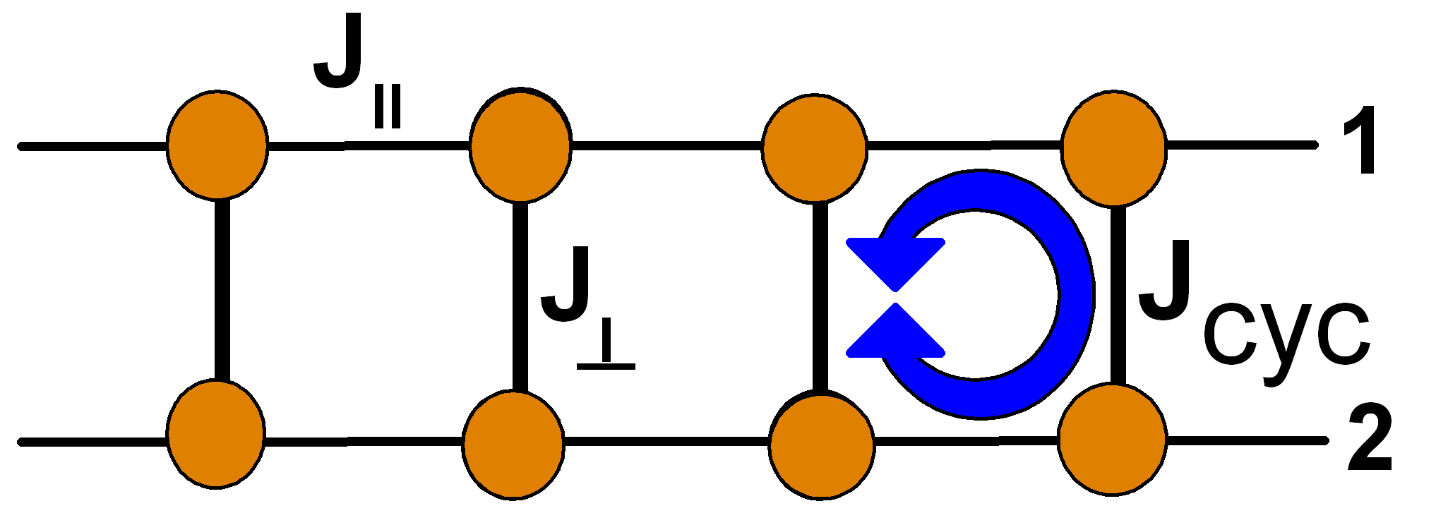
The system we are investigating is a two-leg ladder with localized $S=1/2$ at each vertex, see Ref. Schmidt and Uhrig, 2005 and references therein. The dominant couplings are the antiferromagnetic Heisenberg exchange couplings between nearest neighbours, see Fig. 1. The nearest neighbour exchange couplings are of similar magnitude. The ground state has zero spin and the elementary excitations are of triplet character, i.e., they have $S=1$. Thus we dub them triplons Schmidt and Uhrig (2003) in order to distinguish them from the elementary spin wave excitations, magnons, of systems with magnetic long-range order. The centers of the triplons can be seen to sit on the rungs of the ladder. Further details about the system and its experimental realization will be given in the following sections.

Figure 1: (Color online) Sketch of the two-leg spin ladder. Circles indicate spins with $S=1/2$. Solid lines represent the two-spin exchange couplings on the rungs $J_{\perp}$ and on the legs $J_{\parallel}$. The four-spin cyclic exchange is denoted by $J_{\textrm{cyc}}$.

The temperature development of the spectral weight is induced by two effects. First, the triplons are hardcore bosons so that they can only be created on a rung if there is no other triplon on this rung before. Clearly, this effect depends strongly on temperature because the relative frequency of a successful excitation depends on the concentration of thermally activated triplons. The higher the temperature is the less probable is an excitation process. This effect, due to the hardcore nature, has been dealt with in the preceding investigations as well James et al. (2008); Essler and Konik (2008); James et al. (2009).

Second, triplons can be excited if there are other triplons on rungs nearby. We call this process a conditional excitation henceforth. Thereby, the matrix element for the excitation of a triplon depends on the concentration of thermally activated triplons. It turns out that the sign of the conditional excitations is negative so that higher temperatures and concomitantly higher concentrations of triplons imply a lower spectral weight.

The conditional excitations become more and more important the more the triplons are extended. Hence the vertex corrections due to conditional excitations are significant for isotropic spin ladders where the couplings along rungs and legs of the ladder are of similar magnitude. In the limits investigated previously the vertex corrections did not play a significant role Mikeska and Luckmann (2006); James et al. (2008); Essler and Konik (2008).

We find that the conditional excitations dominate the temperature dependence of the spectral weight. Our theoretical results agree very well with our experimental ones so that evidence for the relevance of these vertex corrections is provided.

Technically, our theoretical calculations are based first on continuous unitary transformations Wegner (1994); Kehrein (2006) which map the original model onto an effective model which conserves the number of excitations Uhrig and Normand (1998); Knetter and Uhrig (2000); Knetter et al. (2003a). This is done in a perturbative fashion where the unperturbed Hamiltonian is given by isolated rungs Knetter et al. (2001); Knetter et al. (2003b). Alternative realizations of degenerate perturbation theory are also based on systematic changes of the underlying basis Trebst et al. (2000); Zheng et al. (2001); J. Oitmaa and Zheng (2006).

Second, we simplify the operators which describe excitation processes by a mean-field (MF) treatment. In this step we focus on a description in terms of single modes.

The paper is set up as follows. In Sect. II we present our model in detail. Subsequently, the theoretical approach is presented in Sect. III. The theoretical results are shown in Sect. IV and compared to experimental results in Sect. V. Finally, the paper is concluded in Sect. VI.

II Model

We study a two-leg $S=1/2$ ladder as it is depicted in Fig. 1. The model is characterized by Heisenberg exchange couplings on the rungs $J_{\perp}$ and on the legs $J_{\parallel}$ of the ladder as well as by a four-spin cyclic exchange $J_{\textrm{cyc}}$. The corresponding Hamiltonian in units of $J_{\perp}$ reads

$$\frac{H}{J_{\perp}} = H_{\perp}+\frac{J_{\parallel}}{J_{\perp}}H_{\parallel}+\frac{J_{\rm cyc}}{J_{\perp}}H_{\rm cyc}$$ (1a)

$$= \sum_{i}\vec{S}_{i,l}\cdot\vec{S}_{i,r}+x\sum_{i;\tau}\vec{S}_{i,\tau}\cdot\vec{S}_{i+1,\tau}+x_{\rm cyc}H_{\rm cyc},\qquad$$ (1b)

where $i$ denotes the rungs and $\tau\in\left\{1,2\right\}$ the upper and lower leg of the ladder. The expansion parameters employed are

$$x := J_{\parallel}/J_{\perp}$$ (2a)

$$x_{\text{cyc}} := J_{\text{cyc}}/J_{\perp}.$$ (2b)

The four-spin ring exchange is given by

$$H_{\textrm{cyc}} = \sum_{i}\left[\left(\vec{S}_{i,l}\cdot\vec{S}_{i+1,l}\right)\left(\vec{S}_{i,r}\cdot\vec{S}_{i+1,r}\right)\right.$$ (3)

$$+\left(\vec{S}_{i,l}\cdot\vec{S}_{i,r}\right)\left(\vec{S}_{i+1,l}\cdot\vec{S}_{i+1,r}\right)$$

$$\left.-\left(\vec{S}_{i,l}\cdot\vec{S}_{i+1,r}\right)\left(\vec{S}_{i+1,l}\cdot\vec{S}_{i,r}\right)\right].$$

These four-spin terms constitute the most important correction to the commonly considered nearest neighbor Heisenberg exchange. By now, this is established for planes Schmidt and Kuramoto (1990); Honda et al. (1993); Müller-Hartmann and Reischl (2002); Reischl et al. (2004) and ladders Brehmer et al. (1999); Mizuno et al. (1999); Matsuda et al. (2000a, b); Schmidt and Uhrig (2005). The size of $J_{\rm cyc}$ in cuprate ladders was found to be of the order 0.2-0.25 $J_{\perp}$ Nunner et al. (2002); Schmidt et al. (2003a); Schmidt et al. (2005); Notbohm et al. (2007). Further corrections like the two-spin interaction over the diagonal are almost one order of magnitude smaller Mizuno et al. (1999) so that they are neglected in the following.

The physics of spin ladders is well understood from the limit of isolated rungs $\{x=0,x_{\rm cyc}=0\}$. In this limit the ground state is the product state of singlets and the excitations are completely local triplets. The elementary excitations at finite values $x$ and $x_{\rm cyc}$ are dressed triplets which are called triplons Schmidt and Uhrig (2003). Triplon excitations are gapped and have total spin one. In the following we will consider triplets on the rungs as local triplons.

It is natural to represent the rung states in terms of bond operators Chubukov (1989a, b); Sachdev and Bhatt (1990). Within this representation, the four-dimensional Hilbert space of each rung $i$ of the ladder is given by the singlet

$$s^{\dagger}_{i}|0\rangle_{i}\!=|s\rangle_{i}\!=\frac{1}{\sqrt{2}}\left(|\!\uparrow\downarrow\rangle-|\!\downarrow\uparrow\rangle\right)$$ (4)

and the three triplet states

$$t^{\dagger}_{-1,i}|0\rangle_{i} \!=|t_{-1}\rangle_{i} \!=\frac{-1}{\sqrt{2}}\left(|\!\uparrow\uparrow\rangle-|\!\downarrow\downarrow\rangle\right)$$ (5a)

$$t^{\dagger}_{0,i}|0\rangle_{i} \!=|t_{0}\rangle_{i} \!=\frac{\mathrm{i}}{\sqrt{2}}\left(|\!\uparrow\uparrow\rangle+|\!\downarrow\downarrow\rangle\right)$$ (5b)

$$t^{\dagger}_{+1,i}|0\rangle_{i} \!=|t_{+1}\rangle_{i} \!=\frac{1}{\sqrt{2}}\left(|\!\uparrow\downarrow\rangle+|\!\downarrow\uparrow\rangle\right).$$ (5c)

The state $|0\rangle=\prod_{i}|0\rangle_{i}$ represents the completely empty system. This is actually an unphysical state which is needed here only for formal reasons.

The physically most important state is the ground state at $\{x=0,x_{\rm cyc}=0\}$ which will be used as a reference state $|{\rm ref}\rangle$ for our calculation. It is given by the product of singlets on all rungs

$$|{\rm ref}\rangle:=\underset{i}{\prod}|s\rangle_{i}.$$ (6)

One can also interpret $|{\rm ref}\rangle$ as a singlet condensate, i.e. singlet operators can be replaced by unity $s=1=s^{\dagger}$ Physically, $|{\rm ref}\rangle$ is the triplon vacuum, i.e., the state without any excitation.

The operator $t^{\dagger}_{\alpha,i}$ with $\alpha\in\left\{0,\pm 1\right\}$ creates an elementary excitation with $S^{z}=\alpha$ (flavor) when applied to a singlet state on rung $i$. Each rung is either occupied by a singlet or by a triplon, resulting in the so called hardcore constraint on all rungs $i$

$$\mathbbm{1}=s_{i}^{\dagger}s^{\phantom{\dagger}}_{i}+\sum_{\alpha}t^{\dagger}_{\alpha,i}t^{\phantom{\dagger}}_{\alpha,i}\quad\alpha\in\left\{-1,0,1\right\},$$ (7)

which implies particle-number conservation in terms of singlets and triplons.

The Hamiltonian (1b) can be reformulated in terms of the above bond operators. One finds

$$H=H_{\perp}+T_{0}+T_{-2}+T_{2}$$ (8)

where the index $n$ in $T_{n}$ indicates the change of the total triplon number, e.g., $T_{+2}\propto t^{\dagger}t^{\dagger}\!ss$ are pair creation processes and $T_{-2}\propto tts^{\dagger}\!s^{\dagger}$ are pair annihilation processes. In contrast, $T_{0}$ does not change the number of triplons in the system. This term includes triplon hopping processes $t^{\dagger}ts^{\dagger}\!s$ and two-triplon interactions $t^{\dagger}t^{\dagger}tt$. Note that we have omitted the spatial and flavor index here in order to keep the notation light. Finally, the operator $H_{\perp}$ counts the total number of triplons in the system.

The low-energy spectrum of spin ladders is well studied Barnes et al. (1993); Gopalan et al. (1994); Greven et al. (1996); Shelton et al. (1996); Oitmaa et al. (1996); Sushkov and Kotov (1998); Eder (1998); Jurecka and Brenig (2000); Trebst et al. (2000); Knetter et al. (2001); Schmidt and Uhrig (2005). All excitations can be classified by the parity with respect to reflections about the centerline of the spin ladder: an odd number of triplons has odd parity and an even number of triplons has even parity.

The most relevant low-energy excitation has odd parity corresponding to a single triplon. It is completely characterized by the one-triplon dispersion

$$\omega(k)=\nu_{0}+2\sum_{m=1}\nu_{m}\cos(mk),$$ (9)

where $k$ is the momentum along the ladder and the $\nu_{m}$ are the one-triplon hopping amplitudes. The dispersion takes a minimum at $k=\pi$ defining the one-triplon gap $\Delta$. In this work we are solely interested in one-triplon energies. Therefore, we do not discuss channels with more triplons. But we note that there are interesting interaction effects present in two-leg ladders leading to two-triplon bound and anti-bound states as well as pronounced continua in their response functions Uhrig and Schulz (1996, 1998); Shelton et al. (1996); Sushkov and Kotov (1998); Damle and Sachdev (1998); Trebst et al. (2000); Jurecka and Brenig (2000); Knetter et al. (2001); Schmidt and Uhrig (2005).

The dynamic structure factor $S^{\alpha,\beta}_{T}(k,\omega)$ is the quantity of interest for inelastic neutron scattering experiments. It is given by

$$S^{\alpha,\beta}_{T}(k,\omega)=\frac{1}{1-e^{-\frac{\omega(k)}{T}}}\,{\rm Im}\,\chi^{\alpha,\beta}_{T}(k,\omega)\quad,$$ (10)

where

$$\chi^{\alpha\beta}_{T}(k,\omega)=i\int_{-\infty}^{\infty}e^{i\omega t}\sum_{r}e^{-ikr}\langle[S_{r}^{\alpha}(t),S_{0}^{\beta}(0)]\rangle\theta(t)$$ (11)

denotes the retarded dynamic susceptibility and the superscripts $\alpha,\beta\in\{\pm 1,0\}$ correspond to the components of the spin. Since our model is SU(2) invariant, the only finite components of the dynamic structure factor are the diagonal ones ($\alpha=\beta$). We define

$$S_{T}(k,\omega)=S^{0,0}_{T}(k,\omega).$$ (12)

The dynamic structure factor at zero temperature is dominated by the one-triplon contribution Knetter et al. (2001); Schmidt and Uhrig (2005). Theoretically, the general form of the one-triplon contribution (or more generically of any single mode (SM) approximation) reads

$$S_{T=0}^{\rm SM}(k,\omega)=a^{2}(k)\delta(\omega-\omega(k)),$$ (13)

where the prefactor $a^{2}(k)$ defines the one-triplon spectral weight which is known to be strongly peaked at the gap momentum $k=\pi$ Uhrig et al. (2004); Schmidt and Uhrig (2005).

III Approach

In this work we are interested in the effects of thermal fluctuations on the one-triplon contribution to the dynamic structure factor of the spin ladder. Physically, one expects that the triplon acquires a finite life-time upon heating. Then the $\delta$-functions at zero temperature are replaced by resonances which are found to show asymmetric line-shapes Essler and Konik (2008).

Our approach is complementary. We do not describe the decay of triplons due to scattering with other thermally excited triplons, but we develop an effective single-mode approximation. That means that the one-triplon contribution to the dynamic structure factor is still given by a $\delta$-function, but with temperature-dependent spectral weight. On the level of the triplon dynamics, this is less sophisticated than the approach by Essler and collaborators James et al. (2008); Essler and Konik (2008); James et al. (2009). In contrast, we are able to efficiently incorporate vertex corrections which are also relevant at finite temperatures. This leads to a temperature-dependent one-triplon spectral weight in our theory.

In the following we give a very short introduction to the method of continuous unitary transformations focusing on the perturbative realization which is used in this work. The acronym CUT stands for the continuous unitary transformations in general and PCUT for their perturbative realization in particular.

We concentrate on the vertex corrections which are relevant for the single-mode description of the finite-temperature dynamic structure factor. For a detailed introduction to CUTs we refer to the literature, see below. In the sequel, we describe the mean-field decoupling of the vertex corrections in detail. They give access to the effective temperature-dependent description of the dynamic structure factor at low energies.

III.1 (P)CUTs

The CUT method was invented independently by Wegner Wegner (1994) and Głazek and Wilson Głazek and Wilson (1993, 1994) in 1994. The CUT itself is defined through the flow equation

$$\partial_{l}H(l)=\left[\eta(l),H(l)\right]$$ (14)

with the continuous parameter $l\in[0,\infty]$ and the initial condition $H(l=0)=H$ where $H$ is the given Hamiltonian. The final form of the effective Hamiltonian $H_{\text{eff}}=H(l=\infty)$ depends on the choice of the infinitesimal generator $\eta$.

Here we use (quasi)particle conserving CUTs Mielke (1998); Uhrig and Normand (1998); Knetter and Uhrig (2000); Fischer et al. (2010) which result in the effective Hamiltonian $H_{\text{eff}}$ being block-diagonal in the number of elementary excitations $q$. In the case of the spin ladder studied, $q$ is the number of excited triplons. In an eigenbasis $|q_{i}\rangle$ ($i$ is an additional index necessary due to degeneracies) of the particle-number operator $Q$ with eigenvalues $q\in\mathbb{N}_{0}$, the generator $\eta^{\rm pc}$ is given by

$$\eta^{\rm pc}_{ij}(l)=\mathrm{sgn}(q_{i}-q_{l})H_{ij}(l).$$ (15)

For the two-leg ladder we choose $J_{\perp}Q=H_{\perp}$ giving an effective Hamiltonian which conserves the number of triplons, i.e., $\left[H_{\perp},H_{\text{eff}}\right]=0$. Consequently, the effective Hamiltonian $H_{\text{eff}}$ decomposes into a sum of irreducible $n$-triplon operators $H_{n}$

$$H_{\text{eff}}=\sum_{n=0}^{\infty}H_{n},$$ (16)

and each $n$-triplon block can be treated separately, see Refs. Knetter et al., 2003a; Fischer et al., 2010 for details.

We apply the CUTs in their perturbative version, i.e., the effective Hamiltonian for the two-leg ladder is obtained as a high-order series expansion in the small parameters

$$x := J_{\parallel}/J_{\perp}$$ (17a)

$$x_{\rm cyc} := J_{\rm cyc}/J_{\perp}.$$ (17b)

The essential one-triplon dispersion $\omega(k)$ has already been determined earlier Schmidt and Uhrig (2005); Knetter et al. (2003a). The one-triplon hopping amplitudes $\nu_{m}$ have been calculated up to order 11 in both perturbative parameters. Various extrapolation schemes can be applied successfully Schmidt et al. (2003b). Especially the low-energy part of the dispersion including the one-triplon gap can be determined very reliably up to realistic values $x\approx 1.25-1.5$ and $x_{\rm cyc}\approx 0.2-0.25$.

In order to calculate spectral properties of the system such as the dynamic structure factor $S_{T}(k,\omega)$ one has to transform observables $O$ by the same CUT as the Hamiltonian. Hence the same generator $\eta^{\rm pc}$ given in Eq. (15) is used

$$\partial_{l}O(l)=\left[\eta^{\rm pc}(l),O(l)\right].$$ (18)

The relevant observable $O(r)$ with odd parity for the dynamic structure factor Schmidt and Uhrig (2005) is given locally on rung $r$ by

$$O(r)=S_{r,1}^{z}-S_{r,2}^{z}=t_{0,r}^{\dagger}s_{0,r}^{\phantom{\dagger}}+t_{0,r}^{\phantom{\dagger}}s_{0,r}^{\dagger}.$$ (19)

The bare observable creates or destroys a single triplon with flavor $0$ on rung $r$. After the CUT, the effective observable $O^{\rm eff}(r)$ comprises many channels reflecting the complicated nature of the interacting triplon problem. One finds

$$O^{\rm eff}(r)=U^{\dagger}O(r)U=\sum_{n,m}O_{n,m}^{\text{eff}}(r)$$ (20)

where $O_{n,m}^{\text{eff}}(r)$ stands for a process where $m$ triplons are annihilated and $n$ are created. Thus $n,m\in\mathbb{N}_{0}$ with the constraint that the difference $n-m$ is an odd number reflecting the odd parity of the observable. At zero temperature, no triplons are present so that only the terms $O_{n,0}$ with $n$ odd are relevant.

Below we need the most relevant one-triplon contribution $O_{1,0}$ which is defined by the one-triplon spectral weights $a^{2}(k)$. The corresponding real space amplitudes have been calculated earlier up to order 10 Schmidt and Uhrig (2005). Extrapolations of the low-energy part close to $k=\pi$ are reliable up to realistic values of $x$ and $x_{\rm cyc}$. The contributions $O_{n,0}$ with $n\geq 3$ are significantly smaller in weight than $O_{1,0}$ Knetter et al. (2001); Schmidt and Uhrig (2005).

At finite temperatures, also contributions $O_{n,m}$ with $m>0$ matter. These contributions give rise to vertex corrections. We will argue below that the most relevant vertex correction for the finite temperature physics at low energies of the spin ladder is the contribution $O_{2,1}$. It comprises processes where a second triplon is created assuming another triplon is already present in the system due to thermal fluctuations. Thus we refer to these processes as conditional excitation processes.

We determined this contribution up to order 9 in the perturbative parameters $x$ and $x_{\text{cyc}}$. For extrapolation, we used the method of internal variables Schmidt et al. (2003c). Unfortunately, no reliable Padé or DlogPadé resummation on top of this extrapolation scheme succeeded, in contrast to the extrapolation of the one-triplon dispersion and the one-triplon spectral weights. Certainly, this fact reflects the more complicated nature of conditional excitations. Nevertheless, we expect that the extrapolation still yields reasonable values for the physical processes up to realistic values of $x$ and $x_{\rm cyc}$.

III.2 Effective single-mode approximation

Next we set up our temperature-dependent theory which results in an effective single-mode approximation. A single-mode contribution to the dynamic structure factor (see Eq. (13)) depends solely on the dispersion and on the spectral weight. The general expression reads

$$S_{T}^{\rm SM}(k,\omega)=\frac{1}{1-e^{-\frac{\omega_{T}(k)}{T}}}\,a_{T}^{2}(k)\,\delta(\omega-\omega_{T}(k)),$$ (21)

where we set the Boltzmann constant $k_{\text{B}}$ to unity, i.e., we measure the temperature in units of energy henceforth.

First, we discuss the temperature effects in the effective dispersion $\omega_{T}(k)$. Second, we incorporate vertex corrections in the spectral weights $a_{T}^{2}(k)$.

III.2.1 Effective dispersion

The one-triplon contribution is characterized at zero temperature by $\omega(k)$. In the PCUT calculation the fully-condensed singlet state $|{\rm ref}\rangle$ with $\langle s^{\dagger}s\rangle=1$ is used as the reference state. Hence no parameter $s<1$ for the singlet occupation needs to be introduced as it was used previously to take the hardcore constraint into account Sachdev and Bhatt (1990); Gopalan et al. (1994). The CUT takes the hardcore constraint into account.

At finite temperatures, however, the situation is different. Even after the CUT there will be a finite occupation of triplons which lowers the singlet occupation. In analogy to the previous studies at zero temperature, we take this effect into account by introducing the mean-field parameter $s(T)$ defined as the condensate value $\langle s^{\dagger}\rangle=s$ with $s\in[0,1]$. We stress the difference to previous studies Sachdev and Bhatt (1990); Gopalan et al. (1994) where $s<1$ was used to consider quantum fluctuations while we use this concept only to consider thermal fluctations. More complex expressions such as $s_{j}^{\dagger}s_{i}^{\phantom{{\dagger}}}$ are reduced to $s^{2}$ which focusses on the average value neglecting fluctuations.

Then the $s$-dependent effective one-triplon dispersion reads

$$\omega_{T}(k,s)=\nu_{0}+2s^{2}(T)\sum_{m=1}\nu_{m}\cos(mk)$$ (22)

because each non-local hopping $t_{\alpha,j}^{\dagger}t_{\alpha,i}^{\phantom{{\dagger}}}$ with $j\neq i$ implies the transfer of a singlet $s_{i}^{\dagger}s_{j}^{\phantom{{\dagger}}}$. The local processes $t_{\alpha,j}^{\dagger}t_{\alpha,j}^{\phantom{{\dagger}}}$ do not require such a renormalization.

To determine the temperature-dependent mean field parameter $s(T)$ it is inserted in the hardcore constraint Eq. (7) yielding

$$1=s^{2}(T)+3\left\langle t^{\dagger}t\right\rangle(T).$$ (23)

So the average triplon occupation $\left\langle t^{\dagger}t\right\rangle(T)$ determines $s(T)$. Due to the spin symmetry the expectation values $\left\langle t_{\alpha}^{\dagger}t_{\alpha}^{\phantom{\dagger}}\right\rangle(T)$ with $\alpha\in\left\{-1,0,1\right\}$ are independent of $\alpha$ resulting in the factor 3 in Eq. (23).

The average triplon occupation can be calculated by the sum over all modes $\langle t_{k}^{\dagger}t_{k}^{\phantom{\dagger}}\rangle$ in momentum space. At finite temperatures one has

$$\left\langle t^{\dagger}_{k}t^{\phantom{\dagger}}_{k}\right\rangle=\frac{1}{Z}\mathrm{Tr}\left(t^{\dagger}_{k}t^{\phantom{\dagger}}_{k}e^{-\frac{H}{T}}\right)=\frac{\partial F}{\partial\omega_{k}}$$ (24)

where $k$ is the triplon momentum. The free energy $F$ is defined via the partition function $Z$ by

$$F=-T\ln(Z)$$ (25)

where $k_{\textrm{B}}$ is set to unity. Integration over the whole Brillouin zone yields the wanted local triplon density

$$\left\langle t^{\dagger}t\right\rangle\left(T\right)=\int_{-\pi}^{\pi}\frac{\left\langle t^{\dagger}_{k}t^{\phantom{\dagger}}_{k}\right\rangle}{2\pi}dk.$$ (26)

If the triplons were bosons without contraint $\left\langle t^{\dagger}_{k}t^{\phantom{\dagger}}_{k}\right\rangle$ would be given by the standard bosonic occupation $(\exp(\omega(k)/T)-1)^{-1}$. Unfortunately, there is no equivalent rigorous expression for hardcore bosons. As an approximate treatment we follow the arguments of Troyer et al. Troyer et al. (1994) to reweight the partition function $Z$ yielding

$$Z = \left(Z_{\omega}\right)^{N}$$

$$Z_{\omega} := 1+\frac{3}{2\pi}\int_{-\pi}^{\pi}e^{-\frac{\omega_{T}(k,s)}{T}}dk$$

where $N$ is the number of rungs. Consequently, the free energy becomes

$$F=-NT\ln\left(1+\frac{3}{2\pi}\int_{-\pi}^{\pi}e^{-\frac{\omega_{T}(k,s)}{T}}dk\right).$$ (28)

Combining Eqs. (28,26,23) yields

$$s^{2}(T)=1-\frac{3}{2\pi}\frac{1}{Z_{\omega}}\int_{-\pi}^{\pi}e^{-\frac{\omega_{T}(k,s)}{T}}dk.$$ (29)

Due to the dependence of the dispersion $\omega_{T}(k,s)$ on $s$ the above equation defines $s$ only implicitly. It has to be evaluated self-consistently.

The value of $s^{2}$ lies in the interval $[0,1]$. Clearly $\lim_{T\to 0}e^{-\frac{\omega_{T}(k,s)}{T}}=0$ as long as $\omega_{T}(k,s)\geq C>0$ which is the physically reasonable case. Hence $s^{2}(T=0)=0$ follows. Similarly, the limit $T\to\infty$ is given by $\lim_{T\to\infty}e^{-\frac{\omega_{T}(k,s)}{T}}=1$ so that $s^{2}(T=\infty)=1/4$ is implied.

For completeness, we mention another effect which implies a renormalization of the effective dispersion due to a finite concentration of thermally excited triplons. Triplon-triplon interactions of the type $t^{\dagger}_{1}t^{\dagger}_{2}t^{\phantom{{\dagger}}}_{3}t^{\phantom{{\dagger}}}_{4}$ are known to exist. For instance, they lead to the occurrence of bound states Windt et al. (2001); Knetter et al. (2001). They also yield some renormalization of the dispersion upon mean-field decoupling

$$t^{\dagger}_{1}t^{\dagger}_{2}t^{\phantom{{\dagger}}}_{3}t^{\phantom{{\dagger}}}_{4} \approx \langle t^{\dagger}_{1}t^{\phantom{{\dagger}}}_{3}\rangle t^{\dagger}_{2}t^{\phantom{{\dagger}}}_{4}+\langle t^{\dagger}_{2}t^{\phantom{{\dagger}}}_{3}\rangle t^{\dagger}_{1}t^{\phantom{{\dagger}}}_{4}$$ (30)

$$+\langle t^{\dagger}_{1}t^{\phantom{{\dagger}}}_{4}\rangle t^{\dagger}_{2}t^{\phantom{{\dagger}}}_{3}+\langle t^{\dagger}_{2}t^{\phantom{{\dagger}}}_{4}\rangle t^{\dagger}_{1}t^{\phantom{{\dagger}}}_{3}+\text{const.},\qquad$$

which is proportional to the triplon densities $\left\langle t^{\dagger}t\right\rangle(T)$. The inclusion of the above terms will renormalize the effective dispersion $\omega_{T}(k)$ slightly. We do not consider the effect of the terms in Eq. (30) here quantitatively for two reasons.

First, an estimate of the quantitative effect of these corrections indicates that they are not very significant. For instance, they are of the same order as the effect of the inclusion of the factor $s^{2}(T)$ in Eq. (22). If this term is omitted no qualitative changes of our results will occur because they are dominated by the renormalization of matrix elements, not by the renormalization of the energies as we will show in the following. Second, their systematic treatment is very tedious because a quantitative determination of all interaction elements would be required.

III.2.2 Vertex corrections and effective spectral weights

Figure 2: Propagation of the excitation included in the calculation. Diagram a) shows the one triplon excitation; diagram b) shows the conditional triplon excitation which requires the existence of a triplon.

The second building block for the one-triplon contribution to the dynamic structure factor is the one-triplon spectral weight. Its unconditional part, active also at zero temperature, is captured by $O_{1,0}^{\text{eff}}$ after the CUT. Its propagation is illustrated diagrammatically in panel a) of Fig. 2. Contributions $O_{n,m}^{\text{eff}}$ with $m>0$ are only active at finite temperatures; they represent conditional excitations. Our idea is to include such contributions as vertex corrections in an effective manner. We identify $O_{2,1}^{\text{eff}}$ as most important because it requires only a single triplon to be present. Hence its quantitative contribution will be proportional to the triplon density. In second quantization $O_{2,1}^{\text{eff}}$ contains operators of the form $t^{\dagger}_{\alpha}t^{\dagger}_{\beta}t^{\phantom{\dagger}}_{\gamma}$. It is illustrated diagrammatically in panel b) of Fig. 2.

Any term of $O_{m+1,m}^{\text{eff}}$ with $m>1$ requires the existence of $m$ triplons so that its quantitative contribution will be proportional to the $m$-th power of the triplon density. In the regime of low temperatures not larger than about the spin gap each additional power in the triplon density stands for another additional exponentially small factor.

Restricting to the two parts $O_{m+1,m}^{\text{eff}}$ with $m\in\{0,1\}$, the effective observable is given by

$$O^{\rm eff}(r) = U^{\dagger}O(r)U$$ (31)

$$\approx O_{1,0}^{\text{eff}}(r)+O_{2,1}^{\text{eff}}(r)$$

$$= \sum_{p}\left(a^{\phantom{\dagger}}_{p}t^{\dagger}_{0,r+p}+\textrm{h.c.}\right)$$

$$+\sum_{\alpha,\beta,\gamma}\sum_{i<j,p}\left(a_{i,j,p}^{\alpha,\beta,\gamma}t^{\dagger}_{\alpha,r+i}t^{\dagger}_{\beta,r+j}t^{\phantom{\dagger}}_{\gamma,r+p}+\textrm{h.c.}\right).\quad$$

The ordering of operators in the above equation is not unique. To avoid double counting, the convention $i<j$ is used. A few excitation processes appearing in $O_{2,1}^{\text{eff}}$ in low order in the small parameters are illustrated in Fig. 3.

Figure 3: (color online) Some conditional excitation processes are sketched which are of low order in $x$. The arrows indicate the rung on which the observable $O_{2,1}^{\text{eff}}(r)$ acts, whereas the cross x denotes the rung which is occupied by the one-triplon before the conditional excitation. Black filled circles denote the rungs occupied by triplons after the conditional excitation process. Open circles are in their singlet state after the excitation; the cyan (gray) part is shown for completeness.

Symmetries of the system imply further constraints. The conservation of the total $S^{z}$ component for processes of the type $t^{\dagger}_{\alpha}t^{\dagger}_{\beta}t_{\gamma}$ lead to

$$0=\alpha+\beta-\gamma\quad\quad\alpha,\beta,\gamma\in\left\{0,\pm 1\right\},$$ (32)

where it is understood that the bare observable is given by Eq. (19).

For scattering experiments we are interested in the Fourier transform of $O^{\rm eff}(r)$ in Eq. (31). For the unconditional contribution $O_{1,0}^{\text{eff}}$ we find

$$\begin{split}O_{1,0}^{\text{eff}}(k)&=\frac{1}{\sqrt{N}}\sum_{r}e^{\mathrm{i}kr}O_{1,0}^{z,\text{eff}}(r)\\ &=\frac{1}{\sqrt{N}}\sum_{r,p}\left(e^{\mathrm{i}kr}a^{\phantom{\dagger}}_{p}t^{\dagger}_{0,r+p}+e^{\mathrm{i}kr}a^{\phantom{\dagger}}_{p}t^{\phantom{\dagger}}_{0,r+p}\right)\\ &=\frac{1}{\sqrt{N}}\sum_{r,p}a^{\phantom{\dagger}}_{p}\left(e^{\mathrm{i}k(r-p)}t_{0,r}^{\dagger}+e^{\mathrm{i}k(r-p)}t^{\phantom{\dagger}}_{0,r}\right)\\ &=a(k)\left(t_{0,-k}^{\dagger}+t^{\phantom{\dagger}}_{0,k}\right)\end{split}$$ (33)

where we use

$$a(k):=\sum_{p}e^{-\mathrm{i}kp}a_{p}.$$ (34)

Note that the coefficients $a_{p}$ are real. For the symmetric spin ladder studied here they are also symmetric $a_{p}=a_{-p}$. The operators $t_{0,k}^{\dagger}$ and $t_{0,k}$ are defined by

$$t_{0,k}^{\phantom{\dagger}} := \frac{1}{\sqrt{N}}\sum_{r}e^{\mathrm{i}kr}t^{\phantom{\dagger}}_{0,r}$$ (35a)

$$t_{0,k}^{\dagger} := \frac{1}{\sqrt{N}}\sum_{r}e^{-\mathrm{i}kr}t^{\dagger}_{0,r}.$$ (35b)

The complete treatment of the conditional excitation is complicated since it involves several sums and the resulting terms are not diagonal in momentum space. We do not, however, aim at the exhaustive description of the multi-particle response, but at the renormalization of the single-mode response. Therefore, we use a mean-field decoupling for $O_{2,1}^{\text{eff}}(k)$ to identify the processes belonging to the creation of a single triplon.

The mean-field decoupling is motivated by Wick’s theorem Wick (1950), but represents an approximation in the present context because the triplons are hardcore bosons. For concentrations of the triplons tending to zero, i.e., for $T\to 0$, the hardcore constraint becomes ineffective and the use of Wick’s theorem is justified

$$t^{\dagger}_{\alpha,i}t^{\dagger}_{\beta,j}t^{\phantom{\dagger}}_{\gamma,p}\approx t^{\dagger}_{\alpha,i}\langle t^{\dagger}_{\beta,j}t^{\phantom{\dagger}}_{\gamma,p}\rangle+t^{\dagger}_{\beta,j}\langle t^{\dagger}_{\alpha,i}t^{\phantom{\dagger}}_{\gamma,p}\rangle.$$ (36)

Due to the symmetry constraint (32) the expectation values are non-zero only for the cases

$$\begin{split}\langle t^{\dagger}_{\beta,j}t^{\phantom{\dagger}}_{\gamma,p}\rangle\neq 0&\quad\text{if}\quad\beta=\gamma\quad\text{and}\quad\alpha=0\\ \langle t^{\dagger}_{\alpha,i}t^{\phantom{\dagger}}_{\gamma,p}\rangle\neq 0&\quad\text{if}\quad\alpha=\gamma\quad\text{and}\quad\beta=0.\end{split}$$ (37)

In all other cases the expectation values are zero. We define the hopping expectation values by

$$\tau^{\phantom{\dagger}}_{T}(j-p):=\langle t^{\dagger}_{\beta,j}t^{\phantom{\dagger}}_{\beta,p}\rangle.$$ (38)

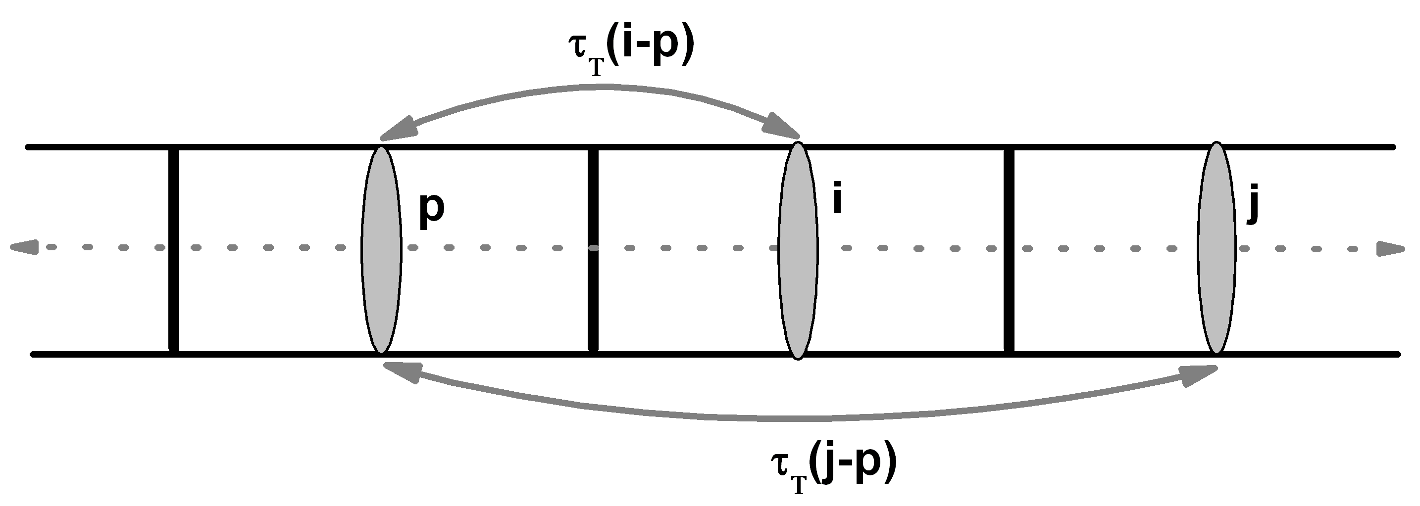
Due to spin rotation symmetry and translation symmetry this definition is independent of $\beta$, but depends only on the relative distance of the two rungs $j$ and $p$ as depicted in Fig. 4. Consequently, we perform an index shift $(j-p)\rightarrow j$ yielding $\tau_{T}(j)$ which is used in the following.

Figure 4: Illustration of the hopping expectation value $\tau_{T}(j-p)$ as defined in Eq. (38).

Employing the mean-field decoupling (36) renders the operator structure of $O_{2,1}^{\text{eff}}$ the same as for $O_{1,0}^{\text{eff}}$. Therefore, Fourier transformation makes it concise

$$O_{2,1}^{\text{eff}}(k) = \frac{1}{\sqrt{N}}\sum_{r,i,j,p}\sum_{\alpha,\beta,\gamma}a_{i,j,p}^{\alpha,\beta,\gamma}\left(e^{\mathrm{i}kr}t^{\dagger}_{\alpha,r+i}t^{\dagger}_{\beta,r+j}t^{\phantom{\dagger}}_{\gamma,r+p}\right.$$ (40)

$$\left.+e^{\mathrm{i}kr}t^{\phantom{\dagger}}_{\alpha,r+i}t^{\phantom{\dagger}}_{\beta,r+j}t^{\dagger}_{\gamma,r+p}\right)$$

$$\approx \frac{1}{\sqrt{N}}\sum_{r,i,j,p}\sum_{\beta}a_{i,j,p}^{0,\beta,\beta}\left(e^{\mathrm{i}kr}t^{\dagger}_{0,r+i}\tau^{\phantom{\dagger}}_{T}(j-p)\delta^{\phantom{\dagger}}_{\beta,\gamma}\right.$$

$$\left.+e^{\mathrm{i}kr}t^{\phantom{\dagger}}_{0,r+i}\tau^{\phantom{\dagger}}_{T}(j-p)\delta^{\phantom{\dagger}}_{\beta,\gamma}\right)$$

$$+\frac{1}{\sqrt{N}}\sum_{r,i,j,p}\sum_{\alpha}a_{i,j,p}^{\alpha,0,\alpha}\left(e^{\mathrm{i}kr}t^{\dagger}_{0,r+j}\tau^{\phantom{\dagger}}_{T}(i-p)\delta^{\phantom{\dagger}}_{\alpha,\gamma}\right.$$

$$\left.+e^{\mathrm{i}kr}t^{\phantom{\dagger}}_{0,r+j}\tau^{\phantom{\dagger}}_{T}(i-p)\delta^{\phantom{\dagger}}_{\alpha,\gamma}\right).$$

Shifting the indices $r\to r-i$ and $j\to j+p$ in the first sum as well as $r\to r-j$ and $i\to i+p$ in the second sum leads to

$$O_{2,1}^{\text{eff}}(k)\ =$$

$$\quad\frac{1}{\sqrt{N}}\sum_{r,i,j,p}\sum_{\beta}a_{i,j+p,p}^{0,\beta,\beta}\left(e^{-\mathrm{i}ki}e^{\mathrm{i}kr}t^{\dagger}_{0,r}\right.$$

$$\ \left.+e^{-\mathrm{i}ki}e^{\mathrm{i}kr}t^{\phantom{\dagger}}_{0,r}\right)\tau^{\phantom{\dagger}}_{T}(j)$$

$$\quad+\frac{1}{\sqrt{N}}\sum_{r,i,j,p}\sum_{\alpha}a_{i+p,j,p}^{\alpha,0,\alpha}\left(e^{-\mathrm{i}kj}e^{\mathrm{i}kr}t^{\dagger}_{0,r}\right.$$

$$\ \left.+e^{-\mathrm{i}kj}e^{\mathrm{i}kr}t_{0,r}\right)\tau^{\phantom{\dagger}}_{T}(i)$$ (41)

$$\overset{(\ref{operatordef})}{=}\sum_{i,j,p}\sum_{\beta}a_{i,j+p,}^{0,\beta,\beta}\left(t^{\dagger}_{0,-k}+t^{\phantom{\dagger}}_{0,k}\right)e^{-\mathrm{i}ki}\tau^{\phantom{\dagger}}_{T}(j)$$

$$\ +\sum_{i,j,p}\sum_{\alpha}a_{i+p,j,p}^{\alpha,0,\alpha}\left(t^{\dagger}_{0,-k}+t^{\phantom{\dagger}}_{0,k}\right)e^{-\mathrm{i}kj}\tau^{\phantom{\dagger}}_{T}(i)$$ (42)

$$=\sum_{i,j,p}\sum_{\alpha}\left(a_{j,i+p,}^{0,\alpha,\alpha}+a_{i+p,j,p}^{\alpha,0,\alpha}\right)\left(t^{\dagger}_{0,-k}+t^{\phantom{\dagger}}_{0,k}\right)e^{-\mathrm{i}kj}\tau^{\phantom{\dagger}}_{T}(i).$$

Finally the full effective observable $O^{\rm eff}(k)$ in momentum space is given by

$$O^{\rm eff}(k) = O_{1,0}^{\text{eff}}(k)+O_{2,1}^{\text{eff}}(k)$$ (43)

$$= \left[a(k)+A_{T}(k)\right]\left(t_{0,-k}^{\dagger}+t^{\phantom{\dagger}}_{0,k}\right),$$

where we used the successive definitions

$$A_{T}(k) := \sum_{i}A_{i}(k)\tau_{T}(i)$$ (44a)

$$A_{i}(k) := \sum_{j}A_{i,j}e^{-\mathrm{i}kj}$$ (44b)

$$A_{i,j} := \sum_{p,\alpha}\left(a_{j,i+p,}^{0,\alpha,\alpha}+a_{i+p,j,p}^{\alpha,0,\alpha}\right).$$ (44c)

Clearly, (43) shows that the conditional excitations imply a renormalization of the spectral weight of the triplons which are the single-mode excitations for the spin ladder. The temperature dependence of $A_{T}(k)$ stems from the temperature dependence of the hopping expectation values $\tau_{T}(j)$. Similar to the calculation of the triplon occupation in (26), the hopping expectation values result from the suitably weighted averages over the Brillouin zone

$$\tau_{T}(j)=\frac{1}{2\pi Z_{\omega}}\int_{-\pi}^{\pi}e^{-\frac{\omega_{T}(k)}{T}}\cos(jk)dk.$$ (45)

The expressions (44) for the effective spectral weights hold for all momenta $k$. But the main effect in the spectral weight is measured at the lowest excitation energy $\Delta:=\omega(\pi)$, i.e., at the momentum $k=\pi$. Hence we restrict ourselves to $k=\pi$ in the following. For $A_{i}(\pi)$ we obtain explicitly

$$A_{i}(\pi) = \sum_{p,j}(-1)^{j}\left(a_{j,i+p,p}^{0,0,0}+a_{i+p,j,p}^{0,0,0}\right.$$ (46)

$$\left.+2\left(a_{j,i+p,p}^{0,1,1}+a_{i+p,j,p}^{1,0,1}\right)\right),$$

where the factor $2$ comes from the fact that $a_{j,i+p,p}^{0,1,1}=a_{j,i+p,p}^{0,-1,-1}$ and $a_{j,i+p,p}^{1,0,1}=a_{j,i+p,p}^{-1,0,-1}$, respectively.

Adding the unconditional and the conditional excitation processes yields the total effective temperature-dependent one-triplon spectral weight at $k=\pi$

$$a^{2}_{T}(\pi)=\big{[}a(\pi)+A^{\phantom{\dagger}}_{T}(\pi)\big{]}^{2}s^{2}(T).$$ (47)

The factor $s^{2}(T)$ stands for the reduced availability of rungs for the creation of triplons if there are already some thermally excited. Putting all pieces together we generalize (13) to finite temperatures

$$S_{T}^{\rm SM}(k,\omega)=a^{2}_{T}(k)\delta(\omega-\omega_{T}(k)),$$ (48)

which we use in the present study for $k=\pi$ only. This is the dynamic structure factor in single-mode approximation of the dynamic structure factor including the vertex corrections relevant at finite temperatures. The physical content of Eq. (48) will be exploited in the next section.

IV Theoretical Results

Next we present our theoretical results obtained by extending the PCUT result to finite temperature using the mean-field (MF) approach. We demonstrate that the intensity decrease in the dynamic structure factor mainly arises from the contribution of the conditional excitations. The basic energy unit in this theory section is chosen to be the rung coupling constant $J_{\perp}$ allowing for direct comparison for different parameter sets $\left\{x,x_{\rm cyc}\right\}$.

In Ref. Notbohm et al., 2007 the parameters $x=1.5$ and $x_{\rm cyc}=0.2-0.25$ were determined to describe a generic cuprate spin ladder best. Thus we chose these parameters to compute the dependence of the self-consistent MF dispersions shown in Fig. 5 with temperature $T$ and wave vector $k$. This provides information on how the shape of the effective dispersion changes upon increasing temperature and momentum. The dispersion becomes flatter on increasing temperature implying a larger energy gap $\Delta(T)=\omega(\pi,T)$.

Figure 5: Effective mean-field dispersion for $x_{\rm cyc}=0.2$ and $x=1.5$ in dependence on temperature and momentum.

Figure 6: (color online) Excitation gap vs. temperature $T$ for $x=\left\{0.75,1,1.25,1.5\right\}$ and a different $x_{\rm cyc}$ in each panel. The red (gray) dots indicate the position of the characteristic temperature $T_{\text{char}}$.

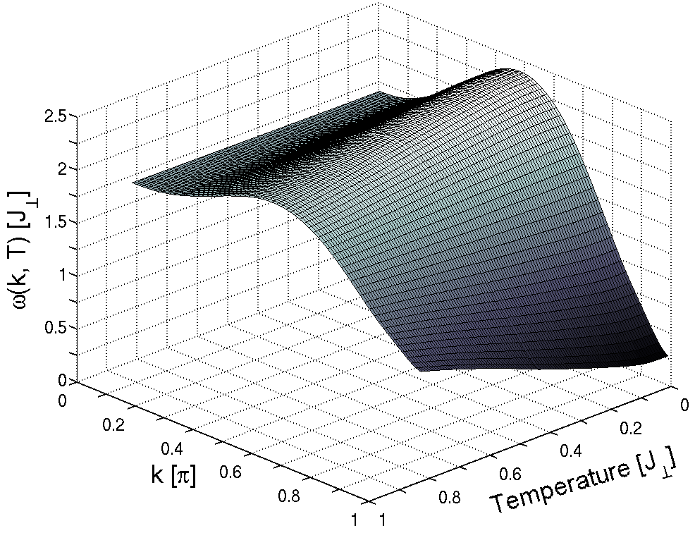
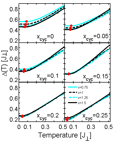
Figure 6 shows the gap as a function of temperature for various $x=\left\{0.75,1,1.25,1.5\right\}$ and a different $x_{\rm cyc}$ in each panel. The blue (gray) dots in each panel indicate a characteristic temperature $T_{\text{char}}$ above which the spin gap shows a significant dependency on temperature in form of a steep gap function $\Delta(T)$ for all $x$ and $x_{\rm cyc}$. The value of $T_{\text{char}}$ scales with the spin gap $\Delta(T=0)$; hence it decreases with increasing $x_{\rm cyc}$.

Three further striking points are to be mentioned. First, with increasing $x_{\rm cyc}$ the curves for $x=\left\{0.75,1,1.25,1.5\right\}$ approach one another until they lie almost on top of one another for $x_{\rm cyc}=0.15-0.2$. For $x_{\rm cyc}=0.25$ they start to spread again. Second, with increasing $x_{\rm cyc}$ the sequence of the curves in each panel changes from $0.75,1,1.25,1.5$ to $1.5,1.25,1,0.75$ from top to bottom. Third, the spin gap $\Delta(T)$ decreases on increasing $x_{\rm cyc}$.

Figure 7: (color online) The dependence of the Average singlet state occupation number $s^{2}(T)$ with temperature for various $x=\left\{0.75,1,1.25,1.5\right\}$ with a different $x_{\rm cyc}$ in each panel.

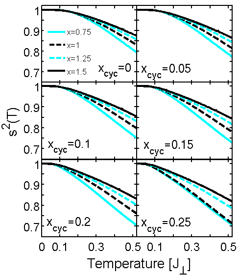
Furthermore, it is interesting how much the average singlet state occupation number $s^{2}(T)$ changes with temperature. Its behaviour is illustrated in Fig. 7. Below the characteristic temperature $T_{\text{char}}$ the occupation number $s^{2}(T)$ is almost independent of temperature for all $x_{\rm cyc}$ resulting from the constant gap energy $\Delta(T)$. Clearly, $T_{\text{char}}$ scales with the energy gap $\Delta(0)$. Above $T_{\text{char}}$ the occupation number $s^{2}(T)$ falls off the steeper the smaller $x$ for a given $x_{\rm cyc}$.

Figure 8: (color online) The upper panel shows the MF triplon hopping expectation value $\tau(j)$ for $j=\left\{0,\dots,6\right\}$ with $x=1.5$ and $x_{\rm cyc}=0.2$. The lower panel depicts the associated conditional MF spectral weight $A_{T}(\pi)$.

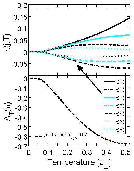
The generic behaviour of the MF triplon hopping excpectation values $\tau(j)$ is depicted in Fig. 8 (upper panel) for $j=\left\{0,\cdots,6\right\}$ vs.  temperature for $x=1.5$ and $x_{\rm cyc}=0.2$. For all other pairs of $x$ and $x_{\rm cyc}$ the hopping expectation values look very similar. The associated conditional MF spectral weight $A_{T}(\pi)$ is shown in the bottom panel of Fig. 8. Thus, the shape of $A_{T}(\pi)$ is dominated by $\tau(j)$ with $j\geq 1$ explaining the minimum in $A_{T}(\pi)$ at about $T=0.514J_{\perp}$ which is about twice the spin gap $\Delta(0)$ .

Figure 9: (color online) One-triplon spectral weight at $k=\pi$, where the spin gap $\Delta(0)$ occurs, for $T=0$ vs. $x$ for various $x_{cyx}$. The one-triplon spectral weight at $k=\pi$ increases on increasing $x$ for fixed $x_{\text{\rm cyc}}$. For fixed $x$ the one-triplon spectral weight increases also on increasing $x_{\text{\rm cyc}}$.

Figure 10: (color online) Conditional MF spectral weight vs.  temperature $T$ for $x=\left\{0.75,1,1.25,1.5\right\}$ and different $x_{\text{cyc}}$ in each panel.

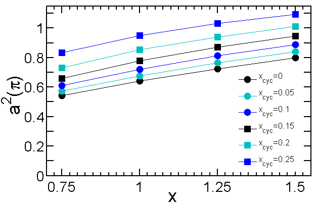
The zero temperature one-triplon spectral weight $a^{2}(\pi)$ vs. $x$ for $x_{\rm cyc}=\left\{0,0.05,0.1,0.15,0.2,025\right\}$ is shown in Fig. 9. With increasing $x$ the one-triplon spectral weight at $k=\pi$ grows. This increasing weight on increasing $x$ confirms the conclusion, that the most important contribution to the one triplon weight and to the conditional triplon excitation weight is found at $k=\pi$. This is the dominant feature in the dynamic structure factor.

Figure 11: (color online) The momentum integrated dynamic structure factor $I(T)=\int S(k,T)\text{d}k$ for $x=\left\{0.75,1,1.2,1.5\right\}$ with a different $x_{\text{\rm cyc}}$ in each panel is presented. It is plotted vs. temperature, normalized to the momentum integrated dynamic structure factor $I_{0}=\int S(k,0)\text{d}k$ at zero temperature.

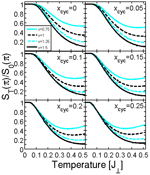
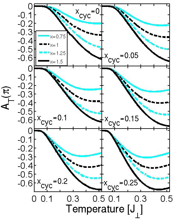
Fig. 10 depicts the conditional MF triplon spectral weight $A_{T}(\pi)$ obtained for various $x=\left\{0.75,1,1.25,1.5\right\}$ and different values $x_{\text{cyc}}$ vs.  temperature. The conditional MF triplon weight for various $x$ shows the expected almost constant behaviour below the characteristic temperature $T_{\text{char}}$ where all curves lie indistinguishably on top of one another. Above $T_{\text{char}}$ a steep fall-off is found. The steepness is affected by the values of $x$ and $x_{\rm cyc}$. The fall-off is the larger the larger $x$ and $x_{\rm cyc}$ are. For fixed $x_{\rm cyc}$ the fall-off becomes stronger on increasing $x$.

The calculated conditional MF amplitude $A_{T}(\pi)$ displays a minimum at about $J_{\perp}/2$ which corresponds to about twice the spin gap $\Delta(0)$. We do not see any physical reason why the weight should increase again. Furthermore, the justification for the approximations involved is less sound beyond temperatures of about $2\Delta(0)$. Life time effects of the modes are expected to become more and more important James et al. (2008); Essler and Konik (2008); James et al. (2009) so that we do not expect the calculated data to be reliable for temperatures beyond $J_{\perp}/2$.

The negative conditional MF amplitude $A_{T}(\pi)$ diminishes the one-triplon spectral weight $a_{T}(k)^{2}$ according to Eq. (47) yielding the normalized momentum-integrated structure factor $\frac{I(T)}{I_{0}}$ presented in Fig. 11. This is the experimentally relevant quantity. The shape of the normalized momentum-integrated structure factor $\frac{I(T)}{I_{0}}$ in Fig. 11 is very similar to the one of the conditional MF spectral weight in Fig. 10 confirming that the conditional excitation process is the dominating effect on increasing temperature. This fact demonstrates the importance of vertex corrections in strongly correlated systems.

V Comparison to Experiment

In an inelastic neutron scattering experiment the dynamic structure factor is measured by the intensity of the scattered neutrons. In order to compare with theory a series of measurements were made on a cuprate spin ladder at different temperatures $T$. These measurements reveal the temperature development of the structure factor.

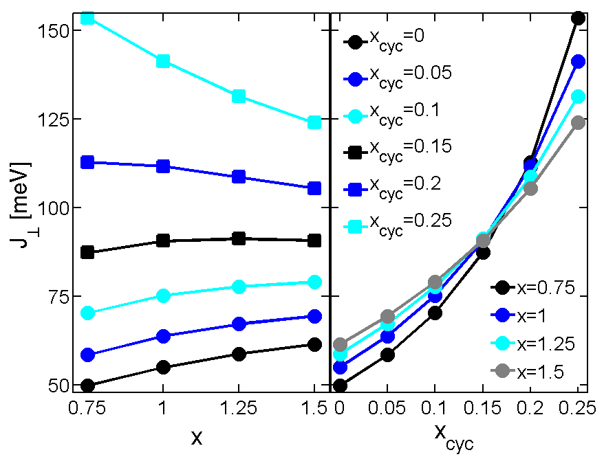
So far we discussed the theoretical results relative to the energy scale given by the coupling constant $J_{\perp}$. In order to compare to experimental data, we have to determine this energy scale. For each pair $\left\{x,x_{\rm cyc}\right\}$ the coupling constant $J_{\perp}$ is determined from the experimental spin gap $\Delta(T=0)=27.6$meV note (2); Notbohm et al. (2007). The obtained values of $J_{\perp}$ are shown in Fig. 12 as functions of $x$ (left panel) and of $x_{\rm cyc}$ (right panel).

A striking point is found in the right panel of Fig. 12 where for $x_{\rm cyc}=0.15$ the value of $J_{\perp}$ is nearly the same for all $x$. The sequence of the curves for various values of $x$ changes at $x_{\rm cyc}=0.15$, i.e., for lower $x_{\rm cyc}$ the curves rise on rising $x$ while they fall for larger $x_{\rm cyc}$. Thus the curve for $x_{\rm cyc}=0.15$ in the left panel of Fig. 12 is almost flat.

Figure 12: (color online) Rung coupling constants $J_{\perp}$ vs. $x$ (left panel) and vs. $x_{\rm cyc}$ (right panel) determined from the experimental energy gap $\Delta(0)=27.6$meV note (2); Notbohm et al. (2007).

V.1 Sample and INS Experiments

Single crystals of La₄Sr₁₀Cu₂₄O₄₁ were grown using the ‘traveling solvent floating zone’ method A. Revcolevschi (1999) at $9$ bar oxygen pressure. INS measurements were performed on the undoped ladder, La₄Sr₁₀Cu₂₄O₄₁ using the MAPS time-of-flight spectrometer at ISIS, Rutherford Appleton Laboratory, U.K. The sample consisted of three co-aligned single crystals with a total mass of 23g (see Ref. Notbohm et al., 2007 for details). The crystals were mounted in a closed cycle cryostat with the $(0kl)$ reciprocal lattice plane horizontal and the $c$ axis perpendicular to the incident neutron beam $k_{i}$. A Fermi chopper was used to select an incident neutron energy of $100$meV and $50$meV and was rotated at a speed of $300$ Hz to give an energy resolution at the elastic line of $4.1$meV and $1.6$meV, respectively. Close to the gap, at an energy transfer of $30$meV the energy resolution is $3.06$meV and $0.93$meV at an incident neutron energy of $100$meV and $50$meV, respectively. Data were collected at temperatures of $15$K, $50$K, $100$K, and $150$K, and of $15$K, $50$K, and $150$K with an incident energy of $100$meV and $50$meV, respectively. Incoherent nuclear scattering from a vanadium standard was used to normalize the magnetic cross-section. In the following text wave vectors $Q_{c}$ and $Q_{a}$ represent the direction along the ladder and along the rung respectively.

V.2 Background Subtraction and Data Analysis

The ladder signal was extracted by taking a constant-$Q$ cut at $Q_{c}=0.5$ and $Q_{a}=1.2$ (wave vector ranges $0.45<Q_{c}<0.55$ and $0.9<Q_{a}<1.5$) where $Q_{c}$ and $Q_{a}$ are given in units of $2\pi/c$ and $2\pi/a$, respectively. The wave vector $Q_{c}=0.5$ corresponds to the position of the gap and the $Q_{a}$ range is chosen to maximise the ratio of magnetic intensity to background due to the rung modulation which goes as $\approx(1-\cos(Q_{a}d_{\text{rung}}))$, where $d_{\text{rung}}$ is the rung distance. The background was determined from a constant-$Q$ cut for the wave vector range $-0.2<Q_{c}<0.2$, and $0.9<Q_{a}<1.5$. This range is appropriate for the determination of the background, because it contains no magnetic scattering due to the ladder structure factor. Each temperature run was treated in exactly the same way, yielding the data shown in Fig. 13.

Figure 13: (color online) Background subtracted ladder signals measured at various temperatures extracted from INS measurements on La₄Sr₁₀Cu₂₄O₄₁. The lower panel shows a zoom of the top panel.

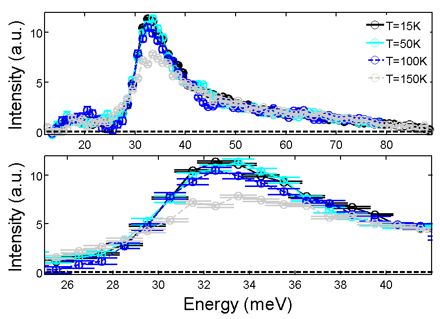
The highest intensity was measured for the coldest run at $15$K. The experiment does not reveal any temperature dependence between $15$K and $50$K. A slight decrease in intensity is observed for $100$K and a significant decrease for $150$K. The spin excitation gap is found to be at $E_{\Delta}=(30\pm 0.5)$meV, see lower panel of Fig. 13, which lies a little lower than that found in Refs. Eccleston et al., 1996; Azuma et al., 1994 and a little higher than found in Ref. Notbohm et al., 2007. Here we define the gap as the energy below the intensity maximum where the scattering strength is half of its maximum value.

The FWHM of the observed peak was extracted by fitting a gaussian to the data. As the real shape of the measured curve deviates from the ideal gaussian, the fit is adjusted such that the gaussian and the data points with an energy below the energy of the maximum intensity match each another. The FWHM values are found to be $5.3\pm 0.5$meV for $15$K, $5.1\pm 0.5$meV for $50$K, $5.3\pm 0.5$meV for $100$K and $(8\pm 0.5)$meV for $150$K for an incident energy of $100$meV and $3.3\pm 0.5$meV for $15$K, $3.5\pm 0.5$meV for $50$K and $(5.8\pm 0.5)$meV for $150$K for an incident energy of $50$meV. Different FWHM values obtained for data collected at the same temperature but different incident energies was due to changes in the energy resolution.

A broadening effect due to damping could therefore only be observed at $150$K. This result confirms that the broadening with increasing temperature is small in comparison to the intensity decrease with increasing temperature, which in turn validates the MF approach presented here. Strikingly the experimental intensity curves in Fig. 13 lie exactly on top of each other above $40$meV for all measured temperatures, indicating that there is a temperature independent tail which we attribute to the wave vector resolution.

The data is compared to the temperature dependent theoretical spectral weight described previously. To determine the relative changes we exclusively used the intensity signal in the range $28\leq\omega\leq 40$meV and calculated the integrated intensities normalized by the area obtained from the $15$K run. Fig. 14 shows the comparison between theory and experiment for the temperature dependent changes of the normalized integrated intensities. The temperature scale is restricted to the temperature region that has been probed experimentally.

Possible pairs of $\left(x,x_{\rm cyc}\right)$ matching the INS data are $\left\{\left(0.75,0.1\right),\left(1,0.15\right),\left(1.25,0.15\right),\left(1.5,0.2\right)\right\}$. However, previous INS measurments Notbohm et al. (2007) and optical conductivity measurements Nunner et al. (2002); Schmidt and Uhrig (2005) showed, that values of $x\approx 1.25-1.5$ and $x_{\rm cyc}\approx 0.20-0.27$ are realistic. To be consistent with previous experimental results we argue that the best agreement within the experimental error bars is found for $x=1.5$ and $x_{\rm cyc}=0.2$ (black solid curve).

Figure 14: (color online) Temperature dependence of normalized dynamic structure factor $\frac{S_{T}(\pi)}{S_{0}(\pi)}$ at $k=\pi$ for various pairs of $\left(x,x_{\text{\rm cyc}}\right)$. The energy scale is set by $J_{\perp}$ given in Tab. 1. The black and red (gray) dots with error bars depict the experimental result obtained from INS for $100$meV and $50$meV, respectively.

$\left(x,x_{\text{cyc}}\right)$	$J_{\perp}\!\left[\text{meV}\right]$
$\left(0.75,0\right)$	$54.2$
$\left(1.5,0\right)$	$66.8$
$\left(0.75,0.1\right)$	$76.4$
$\left(1,0.15\right)$	$98.4$
$\left(1.25,0.15\right)$	$99.1$
$\left(1.25,0.2\right)$	$118$
$\left(1.5,0.2\right)$	$115$
$\left(0.75,0.25\right)$	$166.8$
$\left(1.5,0.25\right)$	$135$

Table 1: Values of the coupling constant $J_{\perp}$ based on a spin gap of $\Delta=30$meV for the various pairs of $\left(x,x_{\text{cyc}}\right)$ for which data is presented in Fig. 14

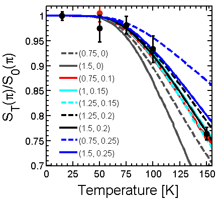
In Ref. Notbohm et al., 2007 $x=1.5$ and $x_{\rm cyc}=0.25$ with $J_{\perp}=124$meV were fitted to the one triplon dispersion extracted from experiment. This little discrepancy in $x_{\rm cyc}$ does not really matter because of the experimental errors and the approximation necessary for computing $A_{T}(\pi)$.

Furthermore, if slightly different energy gaps are assumed, such as $\Delta=35$meV (found in Refs. Eccleston et al., 1996; Azuma et al., 1994), $\Delta=30$meV (present work) and $\Delta=27.6$meV note (2); Notbohm et al. (2007), slightly different results are implied as presented in Fig. 15. Both a gap of $30$meV and of $27.6$meV match the data for realistic parameters $\left\{x,x_{\text{cyc}}\right\}$. In fact, using the spin gap $27.6$meV consistent with the data from Ref. Notbohm et al., 2007 leads to convincing agreement with the values for $\left\{x,x_{\text{cyc}}\right\}$ found in Ref. Notbohm et al., 2007 to fit the INS data. Hence our findings in this work are fully consistent with previous results.

Figure 15: (color online) Normalized spectral weight based on different spin gaps ($\Delta=35$meV (cyan (light gray) lines), $\Delta=30$meV (dark lines), and $\Delta=27.6$meV (blue (dark gray) lines)) is shown. Dashed lines rely on $\left(x,x_{\text{cyc}}\right)=\left(1.5,0.25\right)$ and solid lines on $\left(x,x_{\text{cyc}}\right)=\left(1.5,0.2\right)$. The black and red (dark gray) dots with error bars depict the experimental result obtained from INS for $100$meV and $50$meV, respectively.

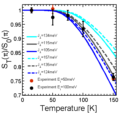
At about half the spin gap energy $\Delta(0)$ our MF theory of vertex corrections predicts a decrease of the spectral weight by $25\%$ for $x=1.5$ and $x_{\rm cyc}=0.2$ with $J_{\perp}=115$meV which agrees very nicely with experiment, see Fig. 15. We stress that a decrease of $25\%$ is well in the regime where we consider our approach valid and reliable.

Note, however, that we omitted the line broadening due to thermal fluctuations in the present analysis which play a more and more important role on increasing temperature. In particular, the unique experimental determination of the weight becomes increasingly difficult.

VI Conclusions

In summary, we derived in this paper vertex corrections in the dynamic structure factor for a quantum antiferromagnet without long range order. The model system investigated is the two-leg spin ladder. The vertex corrections are linked to thermal fluctuations; they are relevant only at finite temperatures. We computed them in the framework of continuous unitary transformations which lead to an effective description of the system in terms of hardcore triplons as elementary excitations.

The vertex corrections are evaluated on the mean-field level, i.e., on the level of a single-model approximation. We found that they induce conditional excitation process which reduce the unconditional, zero-temperature excitation amplitude. Thereby, the spectral weight of the low-lying excitations is diminished because its temperature dependence is indeed found to be dominated by the vertex corrections. The vertex corrections stem eventually from the hardcore character of the triplons. Yet we emphasize that they go beyond the obvious mechanism that no triplon can be excited if its site is already excited by another triplon.

We compared the calculated spectral weight quantitatively with the one measured in the undoped ladder La₄Sr₁₀Cu₂₄O₄₁ using inelastic neutron scattering for a range of temperatures up to $150$K, equivalent to half the spin gap energy. The theory should still apply to considerably higher temperatures as long as these stay below twice the spin gap energy. Experiments at higher temperatures for undoped ladders could test this framework further.

Further research, both theoretical and experimental, on the vertex corrections in other low-dimensional quantum antiferromagnets is called for. In particular, a challenging project consists in the combination of approaches studying the combined effect of line broadening of the single modes James et al. (2008); Essler and Konik (2008); James et al. (2009) and of the vertex corrections.