A factor mixture analysis model for multivariate binary data

Abstract

The paper proposes a latent variable model for binary data coming from an unobserved heterogeneous population. The heterogeneity is taken into account by replacing the traditional assumption of Gaussian distributed factors by a finite mixture of multivariate Gaussians. The aim of the proposed model is twofold: it allows to achieve dimension reduction when the data are dichotomous and, simultaneously, it performs model based clustering in the latent space. Model estimation is obtained by means of a maximum likelihood method via a generalized version of the EM algorithm. In order to evaluate the performance of the model a simulation study and two real applications are illustrated.

KEYWORDS: model based clustering, latent trait analysis, EM algorithm

1 Introduction

Observed binary variables are very common in behavioural and social research. Typical examples are those in which individuals can be classified according to the fact that they agree/disagree to some issues or to the fact that they can choose the right or wrong answer in an educational test. Such binary variables are often supposed to be indicators of one or more latent variables like, for instance, ability or attitude. In the education field latent variables are interpreted as ‘traits’ so that usually factor models for binary data are referred to as latent trait models (Lord and Novick, 1968; Moustaki, 1996). These models can be viewed as a particular class of a more general family of latent variable models classified by Bartholomew and Knott (1999) according to the different nature of manifest and latent variables. When both of them are continuous the latent variable model is the well-known classical factor analysis. When the former are continuous and the latter are discrete we have the latent profile analysis. If both are discrete we refer to the latent class analysis (Lazarsfeld, 1950, Goodman, 1974). With observed discrete variables and continuous latent variables, as in our situation, the latent variable model is called latent trait analysis. The main feature of latent trait models is that the conditional distribution of a complete p-dimensional set of responses of a given individual (called response pattern) is specified as a function of the latent variables. Each of the observed variables follows a Bernoulli conditional distribution, whereas the latent variables are usually assumed to be normally distributed. This assumption cannot be appropriate when the observed data arise from some unobserved sub-populations, so that the investigated population is not homogeneous. In order to detect the potential classes or groups of observations it can be more convenient to consider the latent space as categorical, by performing thus the latent class analysis. According to this approach if a sample of observations arises from some underlying sub-populations of unknown proportions, its distributional form is specified in each of the underlying populations and the purpose is to decompose the sample into its latent classes. For this reason latent class is also referred to as mixture-model clustering (McLachlan and Basford, 1988) or model-based clustering (Banfield and Raftery, 1993; Fraley and Raftery, 2002). For an exhaustive description of latent class analysis see, among the others, Vermunt and Magidson, (2003) and Moustaki and Papageorgiou, (2005).

It is worth noting that the purposes of latent trait and latent class analysis are different. Latent class analysis aims at performing clustering of units whereas the aim of latent trait model is dimension reduction (see Haberman, 1979, and Heinen, 1996, for a further discussion of similarities and differences between the two approaches). When the interest focuses on both issues simultaneously a unified strategy has to be considered.

With this purpose, Everitt (1988) and Everitt and Merette (1990) proposed an extension of model based clustering for mixed data in which the observed categorical variables are generated according to the underlying latent variable approach (Muthén, 1984). Uebersax and Grove (1993) presented a latent trait model for the analysis of agreement on dichotomous or ordered category ratings, in which they assumed a finite mixture of $k=2$ distributions on the univariate latent variable. They also imposed some restrictions on the parameters of the mixture in order to guarantee model estimation through a direct search optimization routine. More recently, a class of latent variable models, called factor mixture models, has been introduced (Yung; 1997, Muthén and Shedden, 1999; Lubke and Muthén, 2005) with the aim of measuring underlying continuous constructs and simultaneously modeling population heterogeneity by incorporating categorical and continuous latent variables. A drawback of this class of methods is that, for assumption, heterogeneity is exclusively ascribed to factor mean differences across the latent classes, while factor variances and covariances are held equal across classes. Montanari and Viroli (2010) proposed an alternative way to deal with unknown heterogeneity by explicitly assuming that the factors underlying a set of continuous observed variables follow a mixture of multivariate Gaussians. In so doing, heterogeneity is fully expressed by factor differences in mean and variance components and the density of the observed variables proves to be a mixture of $k$ heteroscedastic Gaussians, thus improving flexibility and clustering performance.

The aim of this work is to present an extension of heteroscedastic factor mixture analysis (Montanari and Viroli, 2010) for multivariate binary data. The proposed model contextually performs dimension reduction and cluster analysis. Dimension reduction is achieved by assuming that the data have been generated by a factor model with continuous latent variables. In so doing, we measure the ‘traits’ of a latent trait model. Cluster analysis is performed by assuming that the latent variables are modelled as a multivariate Gaussian mixture, thus realizing a model based clustering in the latent space. In this perspective the proposed model can be also viewed as a more general latent trait finite mixture model (Uebersax and Grove; 1993) by allowing heteroscedastic and multivariate mixture components.

The paper is organized as follows. In the next Section the proposed model is introduced and discussed. Section 3 is devoted to model identifiability. A generalized EM algorithm for the estimation of the model parameters is developed and illustrated in Section 4. Section 5 presents the results of a simulation study. Two real applications are finally illustrated.

2 The model

Let $\mathbf{y}=(y_{1},\ldots,y_{p})$ be a vector of $p$ observed binary variables. We assume they are measurements of $q$ latent variables, $\mathbf{z}=(z_{1},\ldots,z_{q})$ or, equivalently, the associations among the observed variables are wholly explained by $q$ latent variables, with $q<p$. The relation between $\mathbf{y}$ and $\mathbf{z}$ can be modelled through a monotone differentiable link function, like the logit, as follows

$$\textrm{logit}(\pi_{j}(\mathbf{z}))=\lambda_{j0}+\sum_{r=1}^{q}\lambda_{jr}z_{r}=\lambda_{j0}+{\boldsymbol{\lambda}}_{j}^{T}\textbf{z}\quad j=1,\ldots,p$$ (1)

where $\pi_{j}(\mathbf{z})=P(y_{j}=1|\mathbf{z})$. The parameters $\lambda_{j0}$ and ${\boldsymbol{\lambda}}_{j}=(\lambda_{j1},\lambda_{j2},\ldots,\lambda_{jq})$ are intercept and factor loadings, respectively, as in the classical factor analysis. Alternatively to the logit, we could have referred to the probit link function (Lord and Novick, 1968).

The joint density function of the response pattern $\mathbf{y}=(1,0,0,\ldots,1)$ is given by

$$f(\mathbf{y})=\int_{R^{q}}f(\mathbf{y}|\mathbf{z})f(\mathbf{z})d\mathbf{z}$$ (2)

where $f(\mathbf{y}|\mathbf{z})$ is the conditional distribution of $\mathbf{y}$ given $\mathbf{z}$ and $f(\mathbf{z})$ is the density function of $\mathbf{z}$. As in the classical factor analysis, we assume that the association among the observed variables is wholly explained by the $q$ latent variables that is the conditional independence of $\mathbf{y}$ given z:

$$f(\mathbf{y}|\mathbf{z})=\prod_{j=1}^{p}f(y_{j}|\mathbf{z})=\prod_{j=1}^{p}\pi_{j}(\mathbf{z})^{y_{j}}[1-\pi_{j}(\mathbf{z})]^{1-y_{j}},$$ (3)

that is, each $f(y_{j}|\mathbf{z})$ follows a Bernoulli distribution. In the classical latent trait model $\mathbf{z}$ is assumed to be multivariate normally distributed. Here, we investigate the alternative assumption that the vector of latent variables z is distributed according to a finite mixture of multivariate Gaussians

$$f(\textbf{z})=\sum_{i=1}^{k}\tau_{i}\phi_{i}^{(q)}({\boldsymbol{\mu}}_{i},{\boldsymbol{\Sigma}}_{i}),$$ (4)

where $\tau_{i}$ are the unknown mixing proportions, $\phi_{i}^{(q)}$ is the Gaussian density with vector mean $\boldsymbol{\mu}_{i}$ and covariance matrix ${\boldsymbol{\Sigma}}_{i}$ of order $q$. This assumption implies that, with respect to the latent variables, the overall population may be heterogeneous and it is composed of $k$ distinct sub-groups, with distribution defined by each Gaussian component. This allows to achieve one of the main aims of this work: the units or individuals may be classified on the basis of their factor values. In particular, clustering is obtained in a dimensionally reduced space defined by the latent traits.

More specifically, clustering is performed by a discrete latent variable we implicitly introduce by modeling the factors through a multivariate mixture of Gaussians. Since its role is to allocate each observation to one out of the $k$ sub-populations of the mixture, it is called allocation variable. The allocation variable is a $k$-dimensional random variable denoted by $\textbf{s}=[s_{i}]_{i=1,\ldots,k}$ following a multinomial distribution

$$f(\textbf{s})=\prod_{i=1}^{k}\tau_{i}^{s_{i}},$$ (5)

and therefore $Pr(s_{1}=0,\ldots,s_{i}=1,\ldots,s_{k}=0)=\tau_{i}$.

Thus the proposed model involves two kinds of latent variables, $\mathbf{z}$ and $\mathbf{s}$, which accomplish the different tasks of dimension reduction and clustering, respectively.

The relation between observed and latent variables can be posed in a hierarchical structure. Since s is related to $\mathbf{y}$ only through $\mathbf{z}$, the so-called complete density of the model $f(\textbf{y},\textbf{z},\textbf{s})$, can be rephrased in the following hierarchical form

$$f(\textbf{y},\textbf{z},\textbf{s}) = f(\textbf{y}|\textbf{z})f(\textbf{z}|\textbf{s})f(\textbf{s}),$$ (6)

which allows to estimate the model by a generalized version of the EM algorithm, that will be presented in the following.

3 Model identifiability

The identifiability of the model is crucial to obtain unique and consistent parameter estimates. The model is not identified when it can be equivalently expressed by different parameterizations. The proposed model (1) can be reformulated in compact form as follows

$$\textrm{logit}(\boldsymbol{\pi}(\mathbf{z}))=\boldsymbol{\lambda}_{0}+{\boldsymbol{\Lambda}}\mathbf{z}$$ (7)

where $\boldsymbol{\pi}(\mathbf{z})=\left(\pi_{1}(\mathbf{z}),\ldots,\pi_{p}(\mathbf{z})\right)$, $\boldsymbol{\lambda}_{0}$ is the $p$-dimensional vector of intercepts and $\boldsymbol{\Lambda}$ is the $p\times q$ matrix of the factor loadings. Notice that (7) is completely indistinguishable from $\textrm{logit}(\boldsymbol{\pi}(\mathbf{z}))=\boldsymbol{\lambda}_{0}+\boldsymbol{\Lambda}\mathbf{M}\mathbf{M}^{-1}\mathbf{z}$, where $\mathbf{M}$ is an invertible square matrix of dimension $q\times q$. In order to avoid this ambiguity and to make the model fully identified $q^{2}$ restrictions have to be imposed (because of the dimension of M).

One solution is the following. As in the classical factor analysis, we assume the factors are standardized, i.e. the mixture parameters must satisfy:

$$E(\textbf{z}) = \sum_{i=1}^{k}\tau_{i}{\boldsymbol{\mu}}_{i}=\textbf{0},$$ (8)

$$Var(\textbf{z}) = \sum_{i=1}^{k}\tau_{i}\left({\boldsymbol{\Sigma}}_{i}+{\boldsymbol{\mu}}_{i}{{\boldsymbol{\mu}}}_{i}^{\top}\right)-\left(\sum_{i=1}^{k}\tau_{i}{\boldsymbol{\mu}}_{i}\right)\left(\sum_{i=1}^{k}\tau_{i}{\boldsymbol{\mu}}_{i}\right)^{\top}=\textbf{I}_{q}.$$ (9)

This implies that the factors are uncorrelated but it is worth noting that they may be mutually dependent, since for non-Gaussian random variables uncorrelatedness does not imply independence and therefore potential nonlinear relationships between the factors are preserved. The previous assumptions introduce $q$ and $q(q-1)/2$ constraints in the estimation of the mean and covariance components, respectively. There are still $q^{2}-q(q+1)/2=q(q-1)/2$ restrictions to be imposed: in fact the model is still invariant under orthogonal rotations. Thus, as proposed by Jöreskog (1969), we introduce the further restrictions on the loading matrix $\boldsymbol{\Lambda}$ by fixing $q(q-1)/2$ loadings equal to 0 (as rule of thumb the upper triangular of $\boldsymbol{\Lambda}$ is fixed to zero).

The previous constraints are necessary and sufficient to obtain the uniqueness of the model solution. A further identifiability aspect to be considered is the existence of the solution. For factor models it is guaranteed by the well-known Lederman’s condition (1937), which relates the number of admissible common factors $q$ to the number of observed variables $p$:

$$k\leq\frac{1}{2}\{2p+1-\sqrt{8p+1}\}.$$ (10)

4 Generalized EM algorithm

In order to develop the EM algorithm for the proposed model a more compact notation must be defined. Let z̃ denote the latent variables with an added column of ones, $\textbf{\~{z}}=(\textbf{1},\textbf{z})$, and $\tilde{\boldsymbol{\Lambda}}$ the matrix of dimension $p\times(q+1)$ which contains also the intercepts. The model parameters are collectively denoted by $\boldsymbol{\theta}=\left\{\boldsymbol{\tilde{\Lambda}},\boldsymbol{\tau},\boldsymbol{\mu},\boldsymbol{\Sigma}\right\}$ where $\boldsymbol{\tau}$ is the vector of $k$ weights, $\boldsymbol{\mu}=(\boldsymbol{\mu}_{1},\ldots,\boldsymbol{\mu}_{k})$ and $\boldsymbol{\Sigma}=(\boldsymbol{\Sigma}_{1},\ldots,\boldsymbol{\Sigma}_{k})$. $\boldsymbol{\theta}$ can be efficiently estimated by the EM algorithm (Dempster et al., 1977). Let ${\textbf{y}}=({\textbf{y}}_{1},...,{\textbf{y}}_{n})$ denote the observed sample of size $n$. The EM algorithm consists of maximizing the conditional expected value of the complete log-likelihood given the observed data:

$$\arg\max_{\boldsymbol{\theta}}E_{\textbf{z},\textbf{s}|\textbf{y},\boldsymbol{\theta}^{\prime}}\left[\log\sum_{h=1}^{n}f\left(\textbf{y}_{h},\textbf{z}_{h},\textbf{s}_{h};\boldsymbol{\theta}\right)\right].$$ (11)

Thanks to the decomposition in (6), the problem simplifies in evaluating the conditional expectation of the logarithm of the three densities and the estimation algorithm has the following structure:

1. Choose starting values $\boldsymbol{\theta}^{\prime}=\left\{\tilde{\boldsymbol{\Lambda}}^{\prime},\boldsymbol{\tau}^{\prime},\boldsymbol{\mu}^{\prime},\boldsymbol{\Sigma}^{\prime}\right\}$.

2. Calculate:

   - $\tilde{\boldsymbol{\Lambda}}$ which maximizes $E_{\textbf{z}|\textbf{y},\boldsymbol{\theta}^{\prime}}\left[\log f(\textbf{y}|\textbf{z};\boldsymbol{\theta})\right]$

   - $\boldsymbol{\mu}$ and $\boldsymbol{\Sigma}$ which maximize $E_{\textbf{z},\textbf{s}|\textbf{y},\boldsymbol{\theta}^{\prime}}\left[\log f(\textbf{z}|\textbf{s};\boldsymbol{\theta})\right]$

   - $\boldsymbol{\tau}$ which maximizes $E_{\textbf{s}|\textbf{y},\boldsymbol{\theta}^{\prime}}\left[\log f(\textbf{s};\boldsymbol{\theta})\right]$

   - Set $\boldsymbol{\theta}^{\prime}=\boldsymbol{\theta}$

3. If convergence is not achieved return to step 2. Convergence is attained when the

   change in the observed data log-likelihood increases by less than a fixed $\epsilon$.

Since all the integrals involved in the expectation step cannot be analytically solved, they are approximated by a weighted sum over a finite number of points with weights given by the Gauss-Hermite quadrature points (see, among the others, Straud and Sechrest, 1966 and Bock and Aitkin, 1981). Thanks to this approximation, estimates for the mixture weights, means, and variance matrices can be obtained in closed form. On the contrary, an analytical estimator for the parameters contained in $\tilde{\boldsymbol{\Lambda}}$ cannot be derived but an iterative Newton-Raphson procedure is needed. This leads to a generalized version of the EM algorithm (GEM, see McLachlan and Krishnan, 2008) whose E and M steps are described in the following.

4.1 E-step

In order to compute the conditional expected value of the complete log-likelihood given the observed data, we need to determine the conditional distribution of the latent variables given the observed data on the basis of provisional estimates of $\boldsymbol{\theta}$, $\boldsymbol{\theta}^{\prime}$:

$$f\left(\textbf{z},\textbf{s}|\textbf{y};\boldsymbol{\theta}^{\prime}\right)=f\left(\textbf{z}|\textbf{y},\textbf{s};\boldsymbol{\theta}^{\prime}\right)f\left(\textbf{s}|\textbf{y};\boldsymbol{\theta}^{\prime}\right).$$ (12)

Using Bayes’ rule, the first term of the previous expression is given by

$$f\left(\textbf{z}|\textbf{y},s_{i}=1;\boldsymbol{\theta}^{\prime}\right)=\frac{f\left(\textbf{z}|s_{i}=1;\boldsymbol{\theta}^{\prime}\right)f(\textbf{y}|\textbf{z};\boldsymbol{\theta}^{\prime})}{f\left(\textbf{y}|s_{i}=1;\boldsymbol{\theta}^{\prime}\right)},$$ (13)

where $f\left(\textbf{z}|s^{(i)}=1\right)$ has the multivariate Gaussian density with vector mean $\boldsymbol{\mu}_{i}$ and covariance matrix ${\boldsymbol{\Sigma}}_{i}$ and $f\left(\textbf{y}|\textbf{z}\right)$ is given in expression (3). However $f(\textbf{y}|s_{i}=1;\boldsymbol{\theta}^{\prime})$ cannot be expressed in closed form and must be approximated. Among the possible approximation methods, Gauss-Hermite quadrature points are used here:

$$f(\textbf{y}|s_{i}=1;\boldsymbol{\theta}^{\prime}) = \int f(\textbf{z}|s_{i}=1;\boldsymbol{\theta}^{\prime})f(\textbf{y}|\textbf{z};\boldsymbol{\theta}^{\prime})d\textbf{z}$$

$$\cong \sum_{t_{1}=1}^{T_{1}}\ldots\sum_{t_{q}=1}^{T_{q}}w_{t_{1}}\ldots w_{t_{q}}f\left(\textbf{y}|\sqrt{2}{\boldsymbol{\Sigma}}_{i}^{1/2}\textbf{z}_{t}+{\boldsymbol{\mu}}_{i};\boldsymbol{\theta}^{\prime}\right)$$

where $w_{t_{1}},\ldots,w_{t_{q}}$ and $\textbf{z}_{t}=(z_{t_{1}},\ldots,z_{t_{q}})^{\top}$ represent the weights and the points of the quadrature respectively.

The second density of expression (12) is the posterior distribution of the allocation variable s given the observed data which can be computed as posterior probability:

$$f(s_{i}=1|\textbf{y};\boldsymbol{\theta}^{\prime})=\frac{f(s_{i}=1;\boldsymbol{\theta}^{\prime})f(\textbf{y}|s_{i}=1;\boldsymbol{\theta}^{\prime})}{\sum_{i=1}^{k}f(s_{i}=1;\boldsymbol{\theta}^{\prime})f(\textbf{y}|s_{i}=1;\boldsymbol{\theta}^{\prime})}.$$ (15)

4.2 M-step

The optimization step (a) of the algorithm consists in evaluating and maximizing:

$$E_{\textbf{z}|\textbf{y};\boldsymbol{\theta}^{\prime}}\left[\log f(\textbf{y}|\textbf{z};\boldsymbol{\theta})\right]=\int\log f(\textbf{y}|\textbf{z};\boldsymbol{\theta})f(\textbf{z}|\textbf{y};\boldsymbol{\theta}^{\prime})d\textbf{z}$$ (16)

with respect to ${\tilde{\boldsymbol{\lambda}}}_{j}=(1,\lambda_{j1},\ldots,\lambda_{jq}$) with $j=1,\ldots,p$, where $f(\textbf{z}|\textbf{y};\boldsymbol{\theta}^{\prime})=\sum_{i=1}^{k}f(s_{i}=1|\textbf{y};\boldsymbol{\theta}^{\prime})f\left(\textbf{z}|\textbf{y},s_{i}=1;\boldsymbol{\theta}^{\prime}\right)$. Notice that $f(\textbf{y}|\textbf{\~{z}};{\boldsymbol{\theta}})=f(\textbf{y}|\textbf{z};{\boldsymbol{\theta}})$. Let $S_{0}({\tilde{\boldsymbol{\lambda}}}_{j},\textbf{y}|\textbf{\~{z}})$ be the derivative with respect to $\tilde{\boldsymbol{\lambda}}_{j}$ of the log-density in (16):

$$S_{0}({\tilde{\boldsymbol{\lambda}}}_{j},\textbf{y}|\textbf{\~{z}})=\frac{\partial\log f({\textbf{y}}|\textbf{\~{z}};{\boldsymbol{\theta}})}{\partial{\tilde{\boldsymbol{\lambda}}}_{j}}=y_{j}\textbf{\~{z}}-\frac{\exp({\tilde{\boldsymbol{\lambda}}}_{j}^{\top}\textbf{\~{z}})\textbf{\~{z}}}{1+\exp({\tilde{\boldsymbol{\lambda}}}_{j}^{\top}\textbf{\~{z}})}.$$

Then the expected score function with respect to the parameter vector $\tilde{\boldsymbol{\lambda}}_{j}$

$$\sum_{i=1}^{k}f(s_{i}=1|\textbf{y};{\boldsymbol{\theta}^{\prime}})\int S_{0}({\tilde{\boldsymbol{\lambda}}}_{j},\textbf{y}|\textbf{\~{z}})f\left(\textbf{\~{z}}|\textbf{y},s_{i}=1;\boldsymbol{\theta}^{\prime}\right)d\textbf{\~{z}}=0$$

can be evaluated by approximating the integrals with Gaussian-Hermite quadrature points:

$$\int S_{0}({\tilde{\boldsymbol{\lambda}}}_{j},\textbf{y}|\textbf{\~{z}})f\left(\textbf{\~{z}}|\textbf{y},s_{i}=1;\boldsymbol{\theta}^{\prime}\right)d\textbf{\~{z}}$$ (18)

$$\cong\frac{1}{f(\textbf{y}|s_{i}=1;\boldsymbol{\theta}^{\prime})}\sum_{t_{1}=1}^{T_{1}}\ldots\sum_{t_{r}=1}^{T_{q}}w_{t_{1}}\ldots w_{t_{q}}S_{0}({\tilde{\boldsymbol{\lambda}}}_{j},\textbf{y}|\textbf{\~{z}}_{t}^{*})f\left(\textbf{y}|\textbf{\~{z}}_{t}^{*};\boldsymbol{\theta}^{\prime}\right)$$

where $\textbf{\~{z}}_{t}^{*}=(1,\textbf{z}_{t}^{*})$ and $\textbf{z}_{t}^{*}=\sqrt{2}{\boldsymbol{\Sigma}}_{i}^{1/2}\textbf{z}_{t}+\boldsymbol{\mu}_{i}$. The approximate gradient offers a non-explicit solution for the not null elements of the parameter vector $\tilde{\boldsymbol{\lambda}}_{j}$, whose estimates can be obtained by applying a constrained matrix in order to take into account the identifiability conditions on $\boldsymbol{\Lambda}$ (see, for major details, Tsonaka and Moustaki, 2007). The estimation problem can be solved by nonlinear optimization methods such as the Newton-type algorithms (Dennis and Schnabel, 1983).

The optimization step (b) of the algorithm consists in optimizing:

$$E_{\textbf{z},\textbf{s}|\textbf{y};\boldsymbol{\theta}^{\prime}}\left[\log f(\textbf{z}|\textbf{s};\boldsymbol{\theta})\right]=\sum_{i=1}^{k}\int\log f(\textbf{z}|\textbf{s};\boldsymbol{\theta})f(\textbf{z},\textbf{s}|\textbf{y};\boldsymbol{\theta}^{\prime})d\textbf{z}$$ (19)

with respect to $\boldsymbol{\mu}_{i}$ and $\boldsymbol{\Sigma}_{i}$. By substituting $f(\textbf{z},\textbf{s}|\textbf{y};\boldsymbol{\theta}^{\prime})=f(s_{i}=1|\textbf{y};\boldsymbol{\theta}^{\prime})f(\textbf{z}|\textbf{y},s_{i}=1;\boldsymbol{\theta}^{\prime})$ in the previous expression, the estimates of the new Gaussian mixture parameters in terms of previous parameters $\boldsymbol{\theta}^{\prime}$ are

$${\boldsymbol{\mu}}_{i} = \frac{f\left(s_{i}=1|\textbf{y};\boldsymbol{\theta}^{\prime}\right)E[\textbf{z}|s_{i}=1,\textbf{y};\boldsymbol{\theta}^{\prime}]}{f\left(s_{i}=1|\textbf{y};\boldsymbol{\theta}^{\prime}\right)},$$

$${\boldsymbol{\Sigma}}_{i} = \frac{f\left(s_{i}=1|\textbf{y};{\boldsymbol{\theta}}^{\prime}\right)\left(E[\textbf{zz}^{\top}|s_{i}=1,\textbf{y};{\boldsymbol{\theta}}^{\prime}]-{\boldsymbol{\mu}}_{i}{\boldsymbol{\mu}}_{i}^{\top}\right)}{f\left(s_{i}=1|\textbf{y};\boldsymbol{\theta}^{\prime}\right)},$$

where the first and second conditional moments, $E[\textbf{z}|s_{i}=1,\textbf{y};\boldsymbol{\theta}^{\prime}]$ and $E[\textbf{zz}^{\top}|s_{i}=1,\textbf{y};\boldsymbol{\theta}^{\prime}]$, can be computed through the Gauss-Hermite quadrature points, similarly to (4.1) and (18). In order to take into account the identifiability conditions given in (8) and (9), the following scaling (20) and centering (21) transformations are performed at each iteration:

$$\boldsymbol{\Sigma}_{i}\rightarrow(\textbf{A}^{-1})^{\top}\boldsymbol{\Sigma}_{i}\textbf{A}^{-1},\ \ \ \boldsymbol{\mu}_{i}\rightarrow(\textbf{A}^{-1})^{\top}\boldsymbol{\mu}_{i}$$ (20)

$$\boldsymbol{\mu}_{i}\rightarrow\boldsymbol{\mu}_{i}-\sum_{i=1}^{k}\tau_{i}\boldsymbol{\mu}_{i},$$ (21)

where A is the Cholesky decomposition matrix of $Var(\textbf{z})$.

Finally, the estimates for the weights of the mixture in step (c) can be computed by evaluating the score function of $E_{\textbf{z},\textbf{s}|\textbf{y};\boldsymbol{\theta}^{\prime}}[\log f(\textbf{s};\boldsymbol{\theta})]$ from which

$${\tau}_{i}=f\left(s_{i}=1|\textbf{y};\boldsymbol{\theta}^{\prime}\right).$$

The algorithm has been implemented in R code and is available from the authors upon request.

5 Model selection

The proposed model is characterized by two unknown dimensional quantities, the number of factors, $q$, and the number of groups, $k$. A possible way to perform model selection is to simultaneously choose $q$ and $k$ on the basis of some information criteria. However, this procedure would require the estimation of all possible combinations of models with $q$ and $k$ varying in a range of admissible values. This would imply a high computational effort, especially when $q$ increases. A possible alternative procedure is inspired by the model assumption that the factors explain all the associations among the observed variables (i.e. conditional independence assumption). This procedure represents a more computationally efficient solution in a forward selection strategy. In more details, it consists of two subsequent steps.

5.1 Choice of the number of factors

First, the most parsimonious models, with $q=1$ and $k$ varying from 1 to a maximum fixed value $K_{\textrm{max}}$, are fitted. If a single factor is not sufficient to explain the associations among the items (for at least one value of $k$), $q$ is increased by one until this condition is satisfied. A possible measure to evaluate if the associations are completely taken into account by $q$ factors, is based on the so-called bivariate residuals (Bartholomew and Knott, 1999, Bartholomew et al., 2002). They quantify the discrepancies between observed and expected frequencies for each bivariate marginal frequency distribution. Any large discrepancies will suggest that the model does not fit the data well. As a rule of thumb a residual greater than 4 is considered large, as suggested by Bartholomew et al. (2002).

The bivariate residual based criterion does not represent the only possible measure considered in the goodness of fit literature for latent trait models. Alternatively classical statistical tests, like the likelihood ratio ($LR$) and the Pearson chi square ($GF$) can be used. However, unlike the classical tests, the bivariate residuals are not affected by the sparseness problem typical of categorical data, as it could occur with several binary items (see, for major details, Reiser, 1996, Bartholomew and On Leung, 2002).

5.2 Choice of the number of components

Once $q$ has been selected, the number of components $k$ can be chosen according to the classical information criteria, such as the well-known BIC (Schwarz, 1978) and AIC (Akaike, 1974). This choice is very important because it is assumed that the number of components coincides with the number of groups. Therefore, the proposed model performs classification of units into $k$ groups in the latent space.

6 Simulation study

The effectiveness of the proposed model is first evaluated on a simulated study in order to analyze the goodness of fit and the classification performance. Six different simulation designs have been implemented by considering $q=1,2,3$ and $k=2,3$. A number of $200$ samples with $n=300$ units have been generated for the different six experimental conditions.

In each experiment, a set of $p=10$ binary variables have been simulated according to the following factor loadings. The intercepts $\boldsymbol{\lambda}_{0}$ have been randomly generated within the range $[-3,3]$ and factor loadings $\boldsymbol{\Lambda}$ have been randomly generated within the interval $[2,4]$ in the case of $q=1$ and for $q>1$ within $[0,0.5]$ and $[2,4]$ for different subsets of items so that a quasi simple structure is produced. The factor parameters have been chosen in order to have quite well-separated and standardized factors as required for the identifiability of the model. For instance, with reference to the simulation design, $q=2$ and $k=3$, the two factors are modelled by a mixture of three multivariate Gaussians with mean and covariance components equal to

$$\mu_{1}=[-1.19\ \ \ 0.77],\ \ \ \ \ \ \ \ \mu_{2}=[1.20\ \ \ 0.76],\ \ \ \ \ \ \ \ \mu_{3}=[-0.01\ \ \ -1.15]$$

$$\boldsymbol{\Sigma}_{1}=\left[\begin{array}[]{rr}0.17&\ 0.08\\ 0.08&0.14\end{array}\right],\ \ \boldsymbol{\Sigma}_{2}=\left[\begin{array}[]{rr}0.16&\ -0.08\\ -0.08&0.12\end{array}\right],\ \ \boldsymbol{\Sigma}_{3}=\left[\begin{array}[]{rr}0.10&\ -0.01\\ -0.01&0.09\end{array}\right]$$

The weights of the mixtures have been fixed equal to $\tau_{1}=0.3$, $\tau_{2}=0.3$ and $\tau_{3}=0.4$. Figure 1 shows the scatterplot of the two factor scores distinguished by group for one of the $200$ simulated samples.

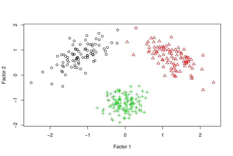
Figure 1: Scatterplot of the factor scores distinguished by group.

For each sample within each experimental design, the previously described GEM-algorithm has been run by initializing the factor loadings with the conventional latent trait analysis solution (with one group). The remaining starting values for the model parameters have been randomly chosen. Eight quadrature points per each dimension have been chosen for the integral approximation.

Table 1 reports the model selection results obtained following the procedure previously described. Columns refer to the different simulation designs. The first three rows contain results about the choice of the number of factors. For each experiment an increasing number of factors has been estimated until the percentage of samples (out of 200 generated samples) with low bivariate residuals is greater than $95\%$. Results show that the correct number of factors is selected in all the experimental conditions.

The remaining rows of the table relates to the choice of $k$, with $q$ given in the previous step. In particular, the percentages with which each fitted model is selected according to BIC and AIC are indicated. According to the BIC the best number of groups is always underestimated with the exception of the first column ($q=1$ and $k=2$) where the true number of groups is chosen most of times. On the contrary, the AIC correctly suggests $k$ in all the six situations. This is due to the fact that the behaviour of the BIC is more conservative than that of AIC because the former is characterized by a heavier penalty term which depends on the sample size and could favour simpler models. Therefore the less restrictive AIC seems to be more appropriate in our situation because of the complexity of the model.

Table 1: Model selection results for 6 different simulation designs. In the first three rows the percentages of samples (out of 200 generated samples) with low bivariate residuals are reported. In the last rows of the table the percentages with which each fitted model is selected according to BIC and AIC are indicated.

	True model specification
	$q=1$		$q=2$		$q=3$
	$k=2$	$k=3$	$k=2$	$k=3$	$k=2$	$k=3$
$q=1$	98%	96%	0%	0%	0%	0%
$q=2$	–	–	100%	100%	0%	0%
$q=3$	–	–	–	–	100%	100%
BIC
$k=1$	38%	20%	82%	4%	96%	31%
$k=2$	43%	51%	18%	69%	4%	68%
$k=3$	16%	27%	0%	27%	0%	1%
$k=4$	3%	2%	0%	0%	0%	0%
AIC
$k=1$	27%	8%	22%	0%	30%	0%
$k=2$	42%	41%	50%	22%	54%	40%
$k=3$	24%	43%	22%	56%	12%	47%
$k=4$	6%	8%	6%	22%	4%	13%

Table 2 reports the means and the root mean square errors (rmse) for the previously described model specification $q=2$ and $k=3$. The factor loading estimates are quite accurate, even if a major precision could be obtained by increasing the sample size and the number of quadrature points. In order to measure the classification performance of the proposed model, the misclassification error between the true class membership and the posterior classification of the estimated model obtained by equation (15) has been computed. The misclassification error mean is 0.131 (with standard error of 0.009), thus indicating that the 86.9% of units are generally correctly classified.

Table 2: In the left part of the table, the true thresholds and factor loadings of the simulated experiment are reported. The middle part of the table contains the means of the thresholds and factor loading estimates across the $200$ samples. In the last part of the table the corresponding root mean square errors are reported.

$\boldsymbol{\lambda}_{0}$	$\boldsymbol{\lambda}_{1}$	$\boldsymbol{\lambda}_{2}$	$\hat{\boldsymbol{\lambda}}_{0}$	$\hat{\boldsymbol{\lambda}}_{1}$	$\hat{\boldsymbol{\lambda}}_{2}$	$\textrm{rmse}_{0}$	$\textrm{rmse}_{1}$	$\textrm{rmse}_{2}$
0.45	2.16	0.00	0.49	2.83	0.00	0.42	1.02	0.00
-0.99	3.21	0.26	-1.04	4.35	0.29	0.71	1.77	0.59
0.11	2.06	0.43	0.14	2.52	0.49	0.33	0.77	0.33
-1.09	3.48	0.16	-1.17	4.70	0.21	0.74	1.83	0.55
-1.57	2.86	0.19	-1.62	3.62	0.26	0.66	1.31	0.51
-0.35	0.03	2.25	-0.40	-0.03	2.64	0.30	0.34	0.62
0.23	0.07	2.22	0.23	0.05	2.62	0.27	0.35	0.70
0.33	0.50	2.42	0.32	0.56	2.83	0.31	0.39	0.76
0.35	0.47	2.25	0.36	0.53	2.73	0.28	0.39	0.85
1.47	0.44	3.68	1.69	0.60	5.19	0.84	0.98	2.16

7 Data Analysis

7.1 Example 1: Attitude towards Abortion

This dataset has been extracted from the 1996 British Social Attitudes Survey (Knott et al., 1990; McGrath and Waterton, 1986). Binary responses to four out of seven items concerning attitude to abortion are given for $379$ individuals. The items investigate circumstances under which an individual would consider that an abortion should be allowed under law. The four circumstances are:

• $y_{1}$: the woman decides on her own that she does not.

• $y_{2}$: the couple agree that they do not wish to have a child.

• $y_{3}$: the woman is not married and does not wish to marry the man.

• $y_{4}$: the couple cannot afford any more children.

Possible responses are coded as 1 for ‘agree’ and 0 for ‘not agree’. Previous analysis (Bartholomew et al., 2002) on this data suggested the presence of two classes in which the response patterns can be grouped. The two classes can be easily interpreted as ‘conservative’ and ‘not conservative’ attitude to abortion, respectively. On the same data, latent trait analysis performed well and highlighted that all the four items are good indicators of a general factor summarizing the attitude towards abortion.

With the proposed model we aim at simultaneously performing a latent trait analysis and grouping the response patterns of the dataset into meaningful classes. To this purpose, a first numerical study has been conducted in order to select among different models with $k$ varying from 1 to 3. As far as the number of factors $q$ is concerned, due to the Lederman’s condition (10), given $p=4$ items only one factor can be estimated in an exploratory context. Moreover, $500$ different starting values for the EM-algorithm have been considered and the best model in terms of number of groups has been chosen according to the AIC criterion (although in this case BIC leads to the same choice). Coherently with the previous results on this data, the information criteria suggest $k=2$.

Table 3: Threshold and loading estimates, with bootstrap standard errors in brackets, attitude to abortion.

Item	$\hat{\lambda}_{i0}$	s.e.	$\hat{\lambda}_{i1}$	s.e.
$y_{1}$	-1.42	(0.067)	5.23	(0.245)
$y_{2}$	0.59	(0.040)	4.45	(0.153)
$y_{3}$	1.27	(0.104)	5.04	(0.301)
$y_{4}$	0.80	(0.056)	3.34	(0.149)

Table 3 reports the threshold and loading estimates. Corresponding standard errors have been obtained by $1000$ bootstrap samples. We can observe that all the loadings are quite similar and significant, confirming that there exists a latent variable common to all of them, which summarizes the opinion pro/anti-abortion of the respondents. This common factor is also used to classify the different response patterns, since it is modelled as a mixture of $k=2$ components. Table 4 shows the clustering results of the fitted model. For comparative purposes, classification obtained by latent class analysis given by Bartholomew et al. (2002) and hierarchical clustering (HC) according to different methods (complete linkage, single linkage and Ward method) is reported. As already mentioned before, latent class analysis distinguishes between two different behaviors of the respondents, those who tend to be in favour of abortion (not conservative group), since they answer ’yes’ at least to two out of the four items and those who are not in favour of abortion (conservative group) since they reply yes to one or none of the four items. On the contrary, if we look at the hierarchical clustering, all the reported methods, a part from the complete linkage one, suggest a more restrictive criterion of classification, that is the conservative group is constituted only by people who respond ‘no’ to all the items. This classification is also suggested by the proposed factor mixture analysis for binary data (FMAB). Thus, the results obtained with FMAB are in agreement with almost all the hierarchical clustering procedures but it is more restrictive than the classical latent class analysis.

Table 4: Class membership for the attitude to abortion data, according to different methods. Columns 2 and 3 are taken from Bartholomew et al. (2002).

Response	LC	Complete	Single	Ward	FMAB
pattern	allocation	HC	HC	HC	allocation
0000	1	1	1	1	1
0001	1	1	2	2	2
0010	1	2	2	2	2
0100	1	1	2	2	2
1000	1	1	2	2	2
0011	2	2	2	2	2
0101	2	1	2	2	2
0110	2	2	2	2	2
1100	2	1	2	2	2
0111	2	2	2	2	2
1011	2	2	2	2	2
1101	2	1	2	2	2
1110	2	2	2	2	2
1111	2	2	2	2	2

7.2 Example 2: American students exposure to school and neighborhood violence

This example has been extracted from the National Longitudinal Survey of Freshmen (NLSF). The NLSF aims at evaluating the academic and social progress of American college students at regular intervals in order to capture emergent psychological processes (by measuring the degree of social integration and intellectual engagement) and to control for pre-existing background differences with respect to social, economic, and demographic characteristics. Data are collected over a period of four waves (1999-2003).
For this analysis we have considered a part of the questionnaire administered in the year 1999 that investigates the freshmen exposure to school and neighborhood violence at age six to ten. It is composed by 21 binary items, 12 of them measuring violence in the schools, the remaining measuring violence in the neighborhood. The items are reported in Table 5.

Table 5: NLSF data: item description.

Item	Question
w1q13a	In your grade school, when you were between the age of six and ten, did you see students fighting?
w1q13b	Students smoking?
w1q13c	Student cutting class?
w1q13d	Students Cutting school?
w1q13e	Students verbally abusing teacher’s?
w1q13f	Did you see physical violence directed at teachers by students?
w1q13g	Vandalism of school or personal property?
w1q13h	Theft of school or personal property?
w1q13i	Students consuming alcohol?
w1q13j	Students taking illegal drugs?
w1q13k	Students carrying knives as weapons?
w1q13l	Students with guns?
w1q14a	In your neighborhood, before you were ten, do you remember seeing homeless people on the street?
w1q14b	Prostitutes on the street?
w1q14c	Gang members hanging on the street?
w1q14d	Drug paraphernalia on the street?
w1q14e	People selling illegal drugs in public?
w1q14f	People using illegal drugs in public?
w1q14g	People drinking or drunk in public?
w1q14h	Physical violence in public?
w1q14i	Hearing the sound of gunshots?

Possible responses are ‘yes’ (coded by 1) or ‘no’ (coded by 0). The original sample was 3924 students of different races. Since we consider several specifications of the proposed latent variable model we reduced computational time by analyzing a random subsample of 400 individuals.
We started with estimating different FMAB models with $q=1$ and $k$ ranging from $1$ to $4$. In all cases the one-factor model is rejected according to both $GF$ and $LR$ test. Also looking at the bivariate residuals there are several pairs of items that present high values, confirming a bad fit. Thus we considered $q=2$ and $k=1,2,3,4$. For these models $GF$ and $LR$ test still indicate that the two-factor model is a poor fit to the data (Table 6), but the bivariate residuals lead to different conclusions. In Table 7 the greatest bivariate residual ($Gffit$) for each pair of responses, for chosen groups $k=3$, are shown (as in the simulation study, the number of groups has been determined according to the AIC criterion, Table 6). We can observe that only one pair of items presents a residual equal to 5.16, indicating that the two latent variables accounts for the pairwise associations and thus that the fit is satisfactory. Evidently, the classical overall goodness of fit tests are strongly affected by sparseness present in the data and this leads to a wrong rejection of the two-factor model.

In the first four columns of Table 8 we reported the loading estimates with associated standard errors in brackets, computed by 1000 bootstrap samples. All the loadings are significant and most of them are negative. We can observe that the items concerning violence in the schools present high negative loadings related to the first factor, whereas the items measuring violence in the neighborhood have high negative loadings in correspondence of the second factor. Thus we can interpret the first factor as “absence of violence in the schools”. The items that strongly influence it are those expressing cutting school (w1q13c and w1q13d) and taking illegal drugs (w1q13j).

On the other hand the second factor can be interpreted as “absence of violence in the neighborhood”. It is interesting to notice that also in this case the items that present the highest loadings are w1q14d and w1q14e, that are the items related to the use and to the traffic of illegal drugs.

Table 6: NLSF data: BIC, AIC, GF and LR for the two-factor model.

$k$	logL	$\sharp par$	BIC	AIC	GF	LR	$df$
1	-2658.257	62	5687.99	5440.51	1007733	904.84	139
2	-2649.596	68	5706.61	5435.19	323533.9	771.76	93
3	-2642.207	74	5727.78	5432.41	786993.6	764.37	81
4	-2643.952	80	5767.22	5447.90	472935.8	766.12	69

Table 7: NLSF data: greatest bivariate residuals for each response, $q=2$, $k=3$.

Response	Items	$Gffit$
(0,0)	7,8	0.59
(0,1)	13,14	3.95
(1,0)	4,12	2.48
(1,1)	8,15	5.16

Table 8: NLSF data: factor loadings with standard errors in brackets: unrotated and rotated solutions.

Items	$\hat{\lambda}_{i1}$	s.e.	$\hat{\lambda}_{i2}$	s.e.
w1q13a	-1.62	(0.01)	0.00	(0.00)
w1q13b	-2.18	(0.04)	0.03	(0.01)
w1q13c	-4.74	(0.22)	0.18	(0.02)
w1q13d	-5.76	(0.26)	0.43	(0.03
w1q13e	-1.74	(0.01)	-0.06	(0.01)
w1q13f	-1.12	(0.01)	-0.25	(0.01)
w1q13g	-1.59	(0.01)	-0.37	(0.01)
w1q13h	-1.45	(0.01)	-0.10	(0.01)
w1q13i	-1.52	(0.88)	-1.56	(0.54)
w1q13j	-8.66	(1.73)	1.72	(0.52)
w1q13k	-1.91	(0.02)	-0.23	(0.01)
w1q13l	-0.81	(0.08)	-0.85	(0.08)
w1q14a	-0.75	(0.01)	-2.06	(0.01)
w1q14b	-0.78	(0.01)	-2.00	(0.02)
w1q14c	-1.36	(0.02)	-3.10	(0.06)
w1q14d	-2.41	(0.05)	-5.08	(0.11)
w1q14e	-3.58	(0.27)	-6.37	(0.45)
w1q14f	-2.44	(0.04)	-3.39	(0.09)
w1q14g	-1.93	(0.02)	-2.62	(0.02)
w1q14h	-2.08	(0.01)	-2.34	(0.01)
w1q14i	-0.85	(0.01)	-1.56	(0.01)

Figure 2 shows the scatterplot of the estimated factor scores distinguished by group. The first cluster, drawn by circles, is constituted by students who present low factor scores for the first latent trait. In other words they are individuals that attended unsafe schools despite the level of safety in the neighborhood. The second cluster, indicated with triangles, is composed by individuals who lived and brought up in no violent environments (both schools and neighborhoods). The third cluster, indicated with crosses, is composed by students who attended schools with little violence but lived in violent neighborhoods.

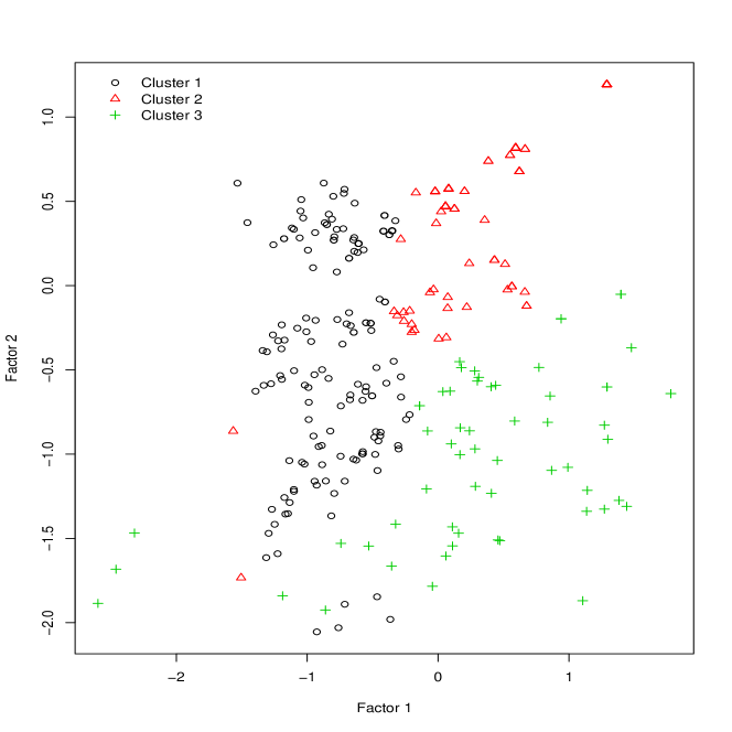
Figure 2: NLSF data: scatterplot of the estimated factor scores distinguished by group.

The three groups of students can be also interpreted by computing the weighted loadings, $\boldsymbol{\Lambda}\boldsymbol{\mu}_{i}$, within each cluster $i$ with $i=1,\ldots,k$, reported in Table 9. In the first group, the weighted loadings are positive for all the items, but higher for those related to school, and therefore for these individuals, on average, the probability of giving answer 1 (presence of violence) is greater than giving answer 0 (absence of violence). The second group of students is characterized by negative weighted loadings and therefore they more likely answer 0. The third group of students is characterized by a contrast between the climate and safety in school and neighborhoods, as previously observed.

Table 9: NLSF data: weighted loadings within each cluster.

	Cluster 1	Cluster 2	Cluster 3
w1q13a	1.29	-0.81	-0.40
w1q13b	1.74	-1.07	-0.58
w1q13c	3.80	-2.30	-1.38
w1q13d	4.66	-2.71	-1.94
w1q13e	1.37	-0.89	-0.35
w1q13f	0.83	-0.65	0.04
w1q13g	1.17	-0.92	0.07
w1q13h	1.12	-0.76	-0.23
w1q13i	0.85	-1.32	1.58
w1q13j	7.27	-3.69	-4.26
w1q13k	1.46	-1.03	-0.18
w1q13l	0.45	-0.71	0.86
w1q14a	0.12	-1.12	2.38
w1q14b	0.16	-1.11	2.30
w1q14c	0.37	-1.80	3.53
w1q14d	0.75	-3.04	5.74
w1q14e	1.38	-4.09	7.06
w1q14f	1.15	-2.44	3.63
w1q14g	0.93	-1.91	2.79
w1q14h	1.11	-1.88	2.40
w1q14i	0.32	-0.99	1.74

8 Discussion

The proposed model combines two methodologies coming from different traditions. Latent trait analysis arose with the aim of evaluating general abilities in education field. Nowadays it represents one of the widest methods to deal with dimension reduction for binary data. On the other hand, Gaussian mixture models have been shown to be a powerful tool for clustering in many applications.
The combination of these two approaches allows to both measure latent factors and to detect potential groups of observations, simultaneously. In particular, clustering is obtained in the dimensionally reduced space defined by the latent traits.

For these reasons it can be viewed as a generalization of the proposal by Uebersax and Grove (1993) by allowing heteroscedastic and multivariate mixture components. A similar approach has been also discussed by Muthèn and Asparouhov (2006) in the context of Item Response Theory (IRT) mixture models. However, differently from our proposal, they do not explicitly assume a semi-parametric distributional form for the latent variables through a mixture of multivariate Gaussians. In addiction we tried fitting a IRT mixture model with Mplus 5 (Muthèn and Muthèn, 2007) on NLSF data with two factors and three classes with the aim of making a comparison with our solution but the algorithm did not achieve convergence.

Results obtained on real data seem to be promising. However, some aspects still need to be investigated. From a computational point of view, the use of a full information maximum likelihood method becomes computationally intensive as the number of latent variables increases. A further challenging aspect for future research is related to the goodness of fit of the model. As already highlighted, the classical tests can be rarely used due to the presence of sparse data. For this reason we referred to the bivariate margins that, although very used in the latent trait analysis, are measures of fit rather than tests. In this sense limited information tests proposed in literature (Reiser, 1996, Maydeu-Olivares and Joe, 2005) could be extended to the proposed model. The analysis could be furthermore extended by considering mixed type of observed variables and, more generally, by putting the model in the framework of generalized linear models.