Nucleation at the DNA supercoiling transition

Abstract

Twisting DNA under a constant applied force reveals a thermally activated transition into a state with a supercoiled structure known as a plectoneme. Using transition state theory, we predict the rate of this plectoneme nucleation to be of order $10^{4}$ Hz. We reconcile this with experiments that have measured hopping rates of order 10 Hz by noting that the viscous drag on the bead used to manipulate the DNA limits the measured rate. We find that the intrinsic bending caused by disorder in the base-pair sequence is important for understanding the free energy barrier that governs the transition. Both analytic and numerical methods are used in the calculations. We provide extensive details on the numerical methods for simulating the elastic rod model with and without disorder.

I Introduction

When overtwisted, DNA forms supercoiled structures known as plectonemes (as seen in the lower right of Fig. 1), familiar from phone cords and water hoses. Single molecule experiments commonly hold a molecule of DNA under constant tension and twist one end; the appearance of a growing plectoneme can be thought of as the nucleation of a new phase that can store some of the added twists as writhe. Recent experiments that hold DNA near this supercoiling transition have shown that it is not initiated by a linear instability (as it is in macroscopic objects), but is rather an equilibrium transition between two metastable states, with and without a plectoneme. These states are separated by a free energy barrier that is low enough to allow thermal fluctuations to populate the two states, but high enough that the characteristic rate of hopping is only about 10 Hz. Two experimental groups, using different methods to manipulate the DNA (one, an optical trap Forth et al. (2008); the other, magnetic tweezers Brutzer et al. (2010)), have observed this nucleation at the transition and reported similar qualitative and quantitative results.

Understanding the rate of plectoneme nucleation at the supercoiling transition is a useful goal for both biology and physics. First, the biological function of DNA is tied to its microscopic physical characteristics, and plectoneme nucleation is sensitive to many of these. The microscopic dynamics of DNA in water is one such factor: while often theorized as a cylindrical rod in a viscous liquid, these dynamics have not been well studied experimentally. The nucleation rate is also sensitive to the intrinsic bend disorder present in a given DNA sequence, potentially providing information to clarify the degree of bend disorder, which is debated in current literature Bednar et al. (1995); Vologodskaia and Vologodskii (2002); Trifonov et al. (1987); Nelson (1998). Popular elastic rod models for DNA can also be tested. Second, DNA supercoiling provides to physics a unique testing ground for theories of thermal nucleation. The theory of thermal nucleation in spatially extended systems (critical droplet theory) was essentially proposed in its current form by Langer in the 1960’s Langer (1968, 1969) (see Hänggi (Hänggi et al., 1990, section IV.F), and also Coleman Coleman (1977) for the corresponding ‘instanton’ quantum tunneling analogue.) Experimental validation of these theories has been difficult in bulk systems, however, for reasons that DNA nucleation neatly bypasses. (a) The nucleation rate in most systems is partly determined by the atomic-scale surface tension; in DNA the continuum theory describes the entire nucleation process. (b) Nucleation in bulk phases is rare (one event per macroscopic region per quench), and hence typically has a high energy barrier. Small estimation errors for this barrier height typically hinder quantitative verification of the (theoretically interesting) prefactor. In single-molecule DNA experiments, the plectoneme nucleation barrier is only a few $kT$, and indeed rather short segments of DNA exhibit multiple hops over the barrier — allowing direct measurements of the transition rate in equilibrium. (c) Nucleation in bulk phases is normally dominated by disorder (raindrops nucleate on dust and salt particles); in DNA the likely dominant source of disorder (sequence-dependence) is under the experimentalist’s control.

As an illustrative example, consider the classic early study of supercurrent decay in thin wires Langer and Ambegokar (1967); McCumber and Halperin (1970). Here (a) the superconductor (like DNA) is well described by a continuum theory (Ginzburg-Landau theory) because the coherence length is large compared to the atomic scale, but (c) the rate for a real, inhomogeneous wire will strongly depend on, for example, local width fluctuations. Finally, (b) the rate of nucleation is so strongly dependent on experimental conditions that an early calculation Langer and Ambegokar (1967) had an error in the prefactor of a factor of $10^{10}$ McCumber and Halperin (1970), but nonetheless still provided an acceptable agreement with experiment.

Reaction-rate theory predicts a rate of plectoneme nucleation related to the energy barrier between the two states. We perform a full calculation of this energy barrier and of the rate prefactor, including hydrodynamics, entropic factors, and sequence-dependent intrinsic bend disorder, to determine which effects contribute to this slow rate. We calculate a rate of order $10^{4}$ Hz, about 1000 times faster than measured experimentally. The discrepancy can be attributed to a slow timescale governing the dynamics of the measurement apparatus. The experiments measure the extension by monitoring the position of a large bead connected to one end of the DNA, and its dynamics are much slower than that of the DNA strand — thus the bead hopping rate that the experiments measure is much slower than the plectoneme nucleation hopping rate that we calculate. Future experiments may be able to slow the plectoneme nucleation rate enough that the bead dynamics is unimportant, such that the bead motion would reveal the dynamic characteristics of the DNA itself.

We begin in section II with the nucleation rate calculation in the absence of disorder: II.1 gives the saddle-point energy, II.2 gives the technique for calculating the prefactor, II.3 overviews the dynamics of DNA in water, and II.4 gives the transition-state theory calculation in full. Section III presents the results of the undisordered calculation, with qualitative explanations of the magnitudes of the various terms, and shows that the results are incompatible with the experiments. This motivates our discussion of base-pair disorder in section IV, where we estimate the disorder-renormalization of the elastic constants in section IV.2, and formulate and calculate the rates in sections IV.3 and IV.4. We conclude in section V.

We draw the reader’s attention in particular to the appendices, where substantive, general-purpose results are presented for numerical discretization and calculations with the elastic rod model. Appendix B reformulates the Euler-angle description in terms of more geometrically natural rotation matrices. Appendix C explains how to transform a DNA with $N$ segments from the $3N$-dimensional Euler-angle or rotation-matrix space to the $4N$-dimensional $(x,y,z,\phi)$ space of the natural dynamics, and the Jacobians needed to transform path integrals over the latter into path integrals over the former. Appendix D discusses the discretization and the rotation-invariant forms for bend and twist in terms of rotation matrices. Finally, Appendix E provides our numerical implementation of randomly-bent DNA, mimicking the effects of a random base-pair sequence.

II Nucleation rate calculation

Figure 1: (Color online) The free energy double-well: A schematic one-dimensional representation of the two metastable states and the saddle point that separates them.

II.1 Saddle point energetics

To understand the dynamics of nucleation, we must first find the saddle point DNA configuration that serves as the barrier between the stretched state and the plectonemic state. We model the DNA as an inextensible elastic rod, with total elastic energy

$$E_{\mathrm{elastic}}=\int_{0}^{L}ds[\frac{B}{2}\beta(s)^{2}+\frac{C}{2}\Gamma(s)^{2}],$$ (1)

where $s$ is arclength along the rod, $\beta$ and $\Gamma$ are the local bend and twist deformation angles, respectively, and $L$ is the contour length of the rod (for more details, see Appendix A; the dynamical equations of motion will be discussed in section II.3). Fain and coworkers used variational techniques to characterize the extrema of this elastic energy functional ; this revealed a “soliton-like excitation” as the lowest-energy solution with nonzero writhe Fain et al. (1997). They found that the soliton’s energy differed from that of the straight state by a finite amount in the infinite-length limit. This soliton state, depicted at the top of the barrier in Fig. 1, is the one we identify as the saddle configuration.

The shape of the saddle configuration is controlled by the bend and twist elastic constants $B$ and $C$, as well as the torque $\tau$ and force $F$ applied as boundary conditions. Defining the lengths

$$a \equiv\sqrt{\frac{B}{F}}$$ (2)

$$b \equiv\frac{2B}{\tau}$$ (3)

$$\ell \equiv(a^{-2}-b^{-2})^{-1/2},$$ (4)

we can write the Euler angles characterizing the saddle configuration as Fain et al. (1997)

$$\cos\theta(s) =1-2\left(\frac{a}{\ell}\right)^{2}\left[1-\tanh^{2}\left(\frac{s}{\ell}\right)\right]$$

$$\phi(s) =\quad\quad\>+\>\frac{s}{b}+\tan^{-1}\left[\frac{b}{\ell}\tanh\left(\frac{s}{\ell}\right)\right]$$ (5)

$$\psi(s) =\frac{s}{C/\tau}-\frac{s}{b}+\tan^{-1}\left[\frac{b}{\ell}\tanh\left(\frac{s}{\ell}\right)\right],$$

where $s$ is arclength along the DNA backbone.

For the experiments in which we are interested, $L/\ell~{}\gg~{}1$ (the soliton “bump” is much smaller than the length of the DNA), such that we can safely remove the soliton from the infinite length solution and still have the correct boundary conditions [$\theta(\pm L/2)=0$, such that the tangent vector $\hat{t}$ points along the $z$ axis at the ends of the DNA]. In this case, the linking number in the saddle state is given by Fain et al. (1997)

$$K_{s} =\frac{1}{2\pi}\left[\phi(L/2)-\phi(-L/2)+\psi(L/2)-\psi(-L/2)\right]$$

$$=\frac{\tau L}{2\pi C}+W_{s}(\tau),$$ (6)

where we have used Eq. (5) and separated the linking number into twist (the first term) and writhe:

$$W_{s}(\tau)=\frac{2}{\pi}\tan^{-1}\left[\frac{b}{\ell}\tanh\left(\frac{L}{2\ell}\right)\right].$$ (7)

To find the saddle configuration’s torque at the supercoiling transition , we numerically solve Eq. (6) for $\tau$ using the experimentally observed critical linking number $K_{s}^{*}$ .

The energy barrier $\Delta E$ is the difference in elastic energy between the saddle and straight states at the same linking number $K_{s}$ . We find

$$\Delta E=\frac{8B}{\ell}\tanh\left(\frac{L}{2\ell}\right)-2\pi W_{s}\left(\tau+\frac{\pi C}{L}W_{s}\right).$$ (8)

Inserting the experimental values listed in Table 1 into Eq. (8), we calculate an energy barrier

$$\Delta E=5.5~{}kT.$$ (9)

This barrier would seem surprisingly small considering that typical atomic rates are on the order of $10^{13}$ Hz: using this for the attempt frequency in an activated rate would give $10^{13}e^{-5.5}=10^{11}$ Hz for the hopping rate. The next sections present a more careful calculation, which shows that the timescale for motion over the barrier is in fact many orders of magnitude smaller than $10^{13}$ Hz due to the larger length scales involved (and even smaller when we calculate the bead hopping rate), but also that the entropy from multiple available nucleation sites significantly lowers the barrier.

Table 1: Parameter values for nucleation rate calculation.

Symbol	Description	Value
$B$	bend elastic constant	(43 nm) $kT$ Forth et al. (2008)
$C$	twist elastic constant	(89 nm) $kT$ Forth et al. (2008)
$F$	applied force	1.96 pN Forth et al. (2008)
$kT$	thermal energy at 23.5∘C	4.09 pN nm
$L$	basepair length of DNA strand	740 nm Forth et al. (2008)
$K_{s}^{*}$	critical linking number	8.7 Forth et al. (2008)
$\tau$	saddle point torque [Eq. (6)]	25 pN nm
$\ell$	soliton length scale [Eq. (4)]	13 nm
$R$	bead radius	250 nm
$\eta$	viscosity of water at 23.5∘C	$9.22\times 10^{-10}$ pN s / nm2
$N$	number of segments	740
$d$	length of segment	1 nm
$r_{D}$	DNA hydrodynamic radius	1.2 nm
$\zeta$	translation viscosity coeff. [Eq. (14)]	$1.54\times 10^{-9}$ pN s / nm2
$\lambda$	rotation viscosity coeff. [Eq. (15)]	$1.67\times 10^{-8}$ pN s

These values have been calculated using $B_{m}=B$, that is, for disorder $D=0$. See Eq. (30).

II.2 Transition state theory: the basic idea

When, as in our case, the energy barrier is much larger than the thermal energy $kT$, the rate of nucleation is suppressed by the Arrhenius factor $\exp{(-\Delta E/kT)}$. Going beyond this temperature dependence to an estimate of the full rate, however, requires a more detailed calculation. We will follow the prescription from Kramers’ spatial-diffusion-limited reaction-rate theory Hänggi et al. (1990) to calculate the rate of hopping. The requirements are that (1) the timescales involved in motion within the two metastable wells are much faster than the timescale of hopping, and (2) (for Kramers’ “spatial-diffusion-limited” theory) the system is overdamped, in the sense that the ratio of damping strength to the rate of undamped motion over the barrier top is large. We check that these requirements are met for the intrinsic DNA nucleation rate after the calculation in section II.4.

Under these two conditions, Kramers’ reaction-rate theory tells us that the rate of hopping over the barrier is controlled only by the rate of motion through the “narrow pass” at the top of the barrier, since it is much slower than any other timescale in the system. This means that the hopping rate should be the characteristic rate of motion across the barrier top times the probability of finding the system near the barrier top, which, in terms of the curvature in the unstable direction away from the saddle point, we can write schematically as

$$k_{\mathrm{hopping}} =\left(\mathrm{Characteristic~{}rate~{}of~{}motion~{}at~{}barrier~{}top}\right)$$

$$\quad\times(\mathrm{Prob.~{}of~{}being~{}at~{}top})$$ (10)

$$=\left(\frac{\mathrm{Energy~{}curvature}}{\mathrm{Damping}}\right)(\mathrm{Prob.~{}of~{}being~{}at~{}top}).$$ (11)

It is important to note that, in current experiments, the measuring apparatus violates condition (1) above. The measurement of the extension is only an indirect readout of the configurational state of the DNA — it is a measure of the position of a large bead connected to one end of the DNA strand. If the bead has much slower dynamics than the DNA, then it will set the characteristic rate of motion in Eq. (10). In section III.4, we will find that this is the case for the experimental numbers we use. Therefore, the rate we will calculate is a plectoneme nucleation hopping rate that is not the same as the (slower) bead hopping rate. We will find also that future experiments may be able to measure the underlying plectoneme nucleation hopping rate by testing regimes where the bead hopping rate is not limited by the bead dynamics.

II.3 Dynamics of DNA in water: the diffusion tensor

To find the rate of motion over the barrier top, we need to know the microscopic dynamics. We will be treating the DNA strand as a series of cylindrical segments, parametrized by the Cartesian coordinates $(x_{n},y_{n},z_{n})$ of one end of each segment plus the Euler angle $\psi_{n}$ that controls local twist (see section C.1 for a discussion about the choice of coordinates). Assuming overdamped motion such that we can neglect inertial terms, we will write the equations of motion in the form [with $\vec{r}_{n}=(x_{n},y_{n},z_{n},\psi_{n})$, $i,j$ labeling coordinates, and $m,n$ labeling segments] Hänggi et al. (1990)

$$\frac{dr_{mi}}{dt}=-M_{mi,nj}\frac{dE}{dr_{nj}};$$ (12)

$M$ is the diffusion tensor, which transforms forces to velocities.

The simplest diffusion tensor produces motion proportional to the local forces, making it diagonal in segment number $n$ and coordinate $i$:

$$M^{\mathrm{diagonal}}_{mi,nj}=\left\{\begin{array}[]{ll}\frac{1}{d\zeta}\,\delta_{mn}\,\delta_{ij}&\mathrm{for}~{}i,j\in\{x,y,z\}\\ \frac{1}{d\lambda}\,\delta_{mn}&\mathrm{for}~{}i=j=\psi\end{array}\right.$$ (13)

The viscous diffusion constants are set so they reproduce the known diffusion constant for a straight cylinder of length $B/kT$ (the bending persistence length) and radius $r_{D}=1.2$ nm: Balaeff et al. (2004); Cox (1970)

$$\zeta =\frac{2\pi\eta}{\ln{(B/(kT\,r_{D}))}}$$ (14)

$$\lambda =2\pi\eta\,r_{D}^{2},$$ (15)

where the viscosity of water $\eta=9.22\times 10^{-10}$ pN s/nm² at the experimental temperature of $23.5^{\circ}$ C.

It is important to note that the DNA in this experiment is attached to a large bead (with radius $R\approx 250$ nm) that must also be pulled through the water during the transition . We take this into account by setting the translational diffusion constant for the final segment in the chain according to Stokes’ Law:

$$M_{Ni,Nj}=\delta_{ij}/(6\pi\eta R)~{}~{}~{}~{}\mathrm{for}~{}i,j\in\{x,y,z\}.$$ (16)

Hydrodynamic effects may also be important, which introduce interactions between segments: as segments move, they change the velocity of the water around them, and this change propagates to change the viscous force felt by other nearby segments. Following Ref. Klenin et al. (1998), we incorporate hydrodynamic effects by using a Rotne-Prager tensor for the translational diffusion, modeling the strand as a string of beads :

$$M^{\mathrm{Rotne-Prager}}_{mi,nj}=\left\{\begin{array}[]{ll}D_{0}\frac{3a}{4r_{mn}}\left[\delta_{ij}+\frac{r_{mn,i}r_{mn,j}}{r_{mn}^{2}}+\frac{2a^{2}}{3r_{mn}^{2}}\left(\delta_{ij}-3\frac{r_{mn,i}r_{mn,j}}{r_{mn}^{2}}\right)\right]\\ \quad\quad\quad\mathrm{for}~{}r_{mn}\geq 2a,~{}m\neq n\\ D_{0}\left[\left(1-\frac{9}{32}\frac{r_{mn}}{a}\right)\delta_{ij}+\frac{3}{32}\frac{r_{mn,i}r_{mn,j}}{a\,r_{mn}}\right]\\ \quad\quad\quad\mathrm{for}~{}r_{mn}\leq 2a,~{}m\neq n\\ D_{0}\,\delta_{ij}~{}\,\mathrm{for}~{}m=n\end{array}\right.$$ (17)

for $i,j\in\{x,y,z\}$, where $D_{0}=(6\pi\eta a)^{-1}$ and $a$ is an effective bead radius chosen such that a straight configuration of Kuhn length $L_{K}=2B/kT$ (with a number of beads $L/L_{K}$) has the same total diffusion constant as a cylinder of length $L$ and radius $r_{D}$ (see Klenin et al. (1998)). With the parameters in Table 1, we use $a=0.98$ nm.

II.4 Transition state theory: full calculation

In the full multidimensional space inhabited by our model, the saddle configuration will have a single unstable direction that locally defines the “reaction coordinate” depicted in Fig. 1. The direction of the unstable mode can be found numerically by locally solving the equations of motion Eq. (12). First, the local quadratic approximation to the energy is provided by the Hessian

$$H_{mi,nj}=\frac{d^{2}E}{dr_{mi}dr_{nj}},$$ (18)

where the derivatives are taken with respect to the unitless variables $\vec{r}={x/\ell_{0},y/\ell_{0},z/\ell_{0},\psi}$ (where $\ell_{0}$ is an arbitrary length scale ; see also section C.1). Inserting the quadratic form defined by $H$ at the saddle point into Eq. (12), we then diagonalize the matrix $MH_{\mathrm{saddle}}$ to find the dynamical normal modes of the system; the single mode $u$ with a negative eigenvalue $-\lambda_{b}$ is the unstable mode at the top of the barrier:

$$M_{li,mj}H^{\mathrm{saddle}}_{mj,nk}\,u_{nk}=-\lambda_{b}\,u_{li},$$ (19)

and $\lambda_{b}$ defines the characteristic rate of Eq. (11). We have checked that we find the correct saddle configuration and unstable mode $u$ by perturbing forward and backward along $u$ and numerically integrating the dynamics of Eq. (12) — one case ends in the straight state well and the other in the plectonemic state well. This generates the transition path connecting the two wells, as illustrated in Fig. 2.

Figure 2: (Color online) Snapshots along the transition path. After perturbing the saddle state along the unstable direction $u$ (bottom left and top right snapshots), we integrate the equations of motion in Eq. (12) to follow the unstable dynamics into the two metastable wells. Here, we use Rotne-Prager dynamics with $D=0$, the timestep between frames is $1.5\times 10^{-6}$ s, and other parameters are as given in Table 1.

To find the probability of being near the top of the barrier in the multidimensional case, we need to know not only the energy barrier $\Delta E$, but also the entropic factors coming from the amount of narrowing in directions transverse to the transition path , which are controlled by the remaining eigenvalues of $H_{\mathrm{saddle}}$ and the Hessian $H_{\mathrm{straight}}$ of the straight state. The full result from spatial-diffusion limited multidimensional transition state theory is (to lowest order in $kT$) Hänggi et al. (1990)

$$k_{\mathrm{hopping}}=\frac{\lambda_{b}}{2\pi}\sqrt{\frac{\det H_{\mathrm{straight}}/(2\pi kT)}{|\det H_{\mathrm{saddle}}/(2\pi kT)|}}e^{-\Delta E/kT};$$ (20)

or, in terms of the eigenvalues of each Hessian,

$$k_{\mathrm{hopping}}=\frac{\lambda_{b}}{2\pi}\sqrt{\frac{\prod_{i=1}^{4(N-2)}\lambda_{i}^{\mathrm{straight}}/(2\pi kT)}{|\prod_{i=1}^{4(N-2)}\lambda_{i}^{\mathrm{saddle}}/(2\pi kT)|}}e^{-\Delta E/kT}.$$ (21)

These are correct if each eigenvalue is sufficiently large such that the local quadratic form is a good approximation where $E\lesssim kT$.

In our case, we must deal separately with the two zero modes due to invariance with respect to location $s_{s}$ and rotation angle $\rho_{s}$ of the saddle configuration’s bump. Extracting these directions from the saddle integral, we have

$$k_{\mathrm{hopping}} =\frac{\lambda_{b}}{2\pi}\left(\int J_{s}J_{\rho}\frac{ds_{s}}{\ell_{0}}d\rho_{s}\right)\sqrt{\frac{\prod_{i=1}^{4(N-2)}\lambda_{i}^{\mathrm{straight}}/(2\pi kT)}{|\prod_{i=3}^{4(N-2)}\lambda_{i}^{\mathrm{saddle}}/(2\pi kT)|}}e^{-\Delta E/kT}$$

$$=\frac{\lambda_{b}}{2\pi}\left(2\pi\frac{L}{\ell_{0}}J_{s}J_{\rho}\right)\frac{1}{2\pi kT}\sqrt{\frac{\det H_{\mathrm{straight}}}{|\det^{\prime}H_{\mathrm{saddle}}|}}e^{-\Delta E/kT},$$ (22)

where the Jacobians $J_{s}=|d\vec{r}_{s}/ds_{s}|$ and $J_{\rho}=|d\vec{r}_{s}/d\rho_{s}|$, and $\det^{\prime}$ represents the determinant without the two zero modes (but including the unstable mode). Numerically, $J_{s}$ and $J_{\rho}$ are calculated using the known forms for derivatives of the saddle point’s Euler angles $\alpha_{s}$ [Eqs. (5)] with respect to $s_{s}$ and $\rho_{s}$: $J_{s}=|[J^{T}(\vec{r}_{s})]^{-1}d\vec{\alpha}_{s}/ds_{s}|$ and $J_{\rho}=|[J^{T}(\vec{r}_{s})]^{-1}d\vec{\alpha}_{s}/d\rho_{s}|$, where $J$ is defined in Eq. (49).

We can now check that we meet the requirements for using Kramers’ theory set out in section II.2. First, we check condition (1) by looking at the smallest nonnegative eigenvalues of $MH$. The slowest mode is transverse motion with wavelength $2L$, and since the bead has much larger viscous drag than the rest of the DNA chain, it sets the damping for this motion; this produces a frequency $F/(6\pi\eta RL)\approx 600$ Hz. The other modes all have frequencies of order $10^{4}$ Hz or faster. We will find that the calculated Kramers rate of hopping lies between these two timescales — this means that, while the bead motion is too slow to follow the fast hopping, Kramers’ theory should correctly give the plectoneme nucleation hopping rate for a fixed bead position. We can check (2) by comparing the characteristic rate for undamped barrier motion to the characteristic damping rate. In the spirit of section III.2, we are dealing with a portion of DNA of length $\ell_{B}$, such that it has a mass $\mu\ell_{B}$, where $\mu=3.3\times 10^{-21}$ g/nm is the linear mass density of DNA Mülhardt (2006), and the energy curvature at the barrier top is on the order of $\pi^{4}B/\ell_{B}^{3}$. Then the damping coefficient is $\zeta/\mu=5\times 10^{11}~{}\mathrm{s}^{-1}$, and the rate for undamped barrier motion is $\sqrt{(\pi^{4}B/\ell_{B}^{3})/(\mu\ell_{B})}=4\times 10^{8}~{}\mathrm{s}^{-1}$. Since the ratio of these values is much greater than one, we are firmly in the overdamped regime, and Kramers’ rate theory applies Hänggi et al. (1990).

III Initial results and order of magnitude checks

III.1 Initial results

We calculate the rate in Eq. (22) using numerical methods described in the Appendices. We will quote the results of the calculation by looking individually at the factors that contribute to the rate. Writing the rate in various simple forms,

$$k_{\mathrm{hopping}} =\frac{\lambda_{b}}{2\pi}e^{-\Delta E/kT+S/k}$$ (23)

$$=\frac{\lambda_{b}}{2\pi}e^{-\Delta\mathcal{F}/kT};$$ (24)

$S$ encapsulates the entropic factors coming from fluctuations in the straight and saddle configurations, and the effective free energy barrier $\Delta\mathcal{F}=\Delta E-TS$ provides the relative probability of being near the top of the saddle Hänggi et al. (1990).

Figure 3: (Color online) Transition state theory plectoneme nucleation hopping rate (bottom) and the factors that contribute to that rate (top) versus external force. (Blue; lower) Energetic factor $\exp{(-\Delta E/kT)}$; (Red; middle) entropic factor $\exp{(S/k)}$; (Green; upper) dynamic factor $\lambda_{b}/2\pi$, in Hz; (Black) the final hopping rate per unit length from Eq. (22). The calculation is performed for the experimental conditions in Ref. Forth et al. (2008), with $L=2.2$ kbp (squares) and $L=4.2$ kbp (diamonds). On this log scale, adding the three distances from the horizontal line at $10^{0}$ in the top plot produces the final rate. Note that the entropic factor cancels the slowing from the energy barrier factor. (Here the calculation is performed without intrinsic bend disorder, producing small or even negative free energy barriers — see section IV.)

For the experimental parameters in Table 1, using Rotne-Prager dynamics , we find $\lambda_{b}/2\pi=4.0\times 10^{4}$ Hz, $\Delta E/kT=5.5$, and $S/k=5.8$, such that $\Delta\mathcal{F}/kT~{}=~{}-0.3$. There are two surprises here: (1) the characteristic rate of motion over the barrier is very slow compared to typical atomic timescales, and (2) the entropic factors are so large that they completely erase the energy barrier. We consider these issues in more detail in the next three sections. We will find that the slow characteristic rate comes from the larger length scales involved in the transition, and that entropy wins over energy due to the length of the DNA. (Roughly speaking, since we calculate a probability per unit length of a plectoneme critical nucleus, for long enough DNA there will always be such a nucleus.)

These rate factors and the corresponding rate per unit length of DNA are plotted as a function of external force for the two experimentally-measured lengths in Fig. 3 . This rate per unit length itself depends on the length because (1) the saddle-state torque $\tau$ changes with $L$ and (2) the twisting component of the unstable mode $d\psi$ is length-dependent at the lengths of interest .

III.2 Order of magnitude estimates of the dynamical prefactor

Typically, rates for atomic scale systems have prefactors on the order of $10^{13}$ Hz. Indeed, inserting typical atomic length scales (Å) and energy scales (eV) into the simple rate equation Eq. (11), and using Stokes’ law for an angstrom sized sphere in water, the energy curvature is $1$ eV/Ų, and the damping is $6\pi\eta r_{a}=10^{-13}$ eV s/Ų, producing a dynamical prefactor of $10^{13}$ Hz.

Why, then, is our dynamical prefactor of order $10^{4}-10^{5}$ Hz? It turns out that the relevant length and energy scales for the DNA supercoiling transition are not atomic. For the saddle state, we are dealing with length scales on the order of tens of nanometers (much larger than single atoms), and energy scales related to the elastic constants ($B/\ell\approx 10$ pN nm $<0.1$ eV).

Figure 4: (Color online) Unstable mode at top of barrier. (top) The four components of the unstable mode eigenvector as a function of arclength $s$ along the DNA strand. (bottom) Plot of $dr=\sqrt{dx^{2}+dy^{2}+dz^{2}}$; the peaks show the locations where the (Cartesian) motion of the DNA is greatest when traversing the barrier. Note that the width of the peak is about 75 nm — inserting this length scale into Eq. (25) produces a prefactor $\sim~{}10^{5}$ Hz.

To arrive at a better estimate, we can approximate the saddle energetics from bending energies only. Consider approximating the saddle state as a straight configuration with a single planar sinusoidal bump of length $\ell_{B}$ and amplitude $A$. Since the elastic bending energy is $E_{B}=\frac{B}{2}\int(\frac{dt}{ds})^{2}ds$, where the relevant component of the tangent vector is in this case $t=Ak_{t}\cos{(k_{t}s)}$ for wavenumber $k_{t}=\pi/\ell_{B}$, the total bending energy for the bump is $E_{B}=\frac{B\ell_{B}}{2}k_{t}^{4}A^{2}=\frac{\pi^{4}B}{\ell_{B}^{3}}\frac{A^{2}}{2}$; this leads to an energy curvature with respect to amplitude of $d^{2}E_{B}/dA^{2}=\frac{\pi^{4}B}{\ell_{B}^{3}}$. The viscous damping coefficient corresponding to a rod of radius $r_{D}$ and length $\ell_{B}$ moving sideways through water is $\ell_{B}\zeta$, with $\zeta$ given by Eq. (14). Putting this together, our back-of-the-envelope estimate for the prefactor is [see Eq. (11)]

$$\frac{\mathrm{Energy~{}curvature}}{\mathrm{Damping}}\sim\frac{\pi^{4}B}{\ell_{B}^{4}\zeta}.$$ (25)

We see that the prefactor is strongly dependent on the length scale $\ell_{B}$ of the bending of DNA in the unstable mode motion. This length scale should be related to the length $\ell\sim 10$ nm, defined in Eq. (4), characterizing the shape of the saddle configuration. As shown in Fig. 4, we can check the amount of DNA involved in the unstable mode motion by looking at the unstable mode eigenvector. This reveals that a better estimate for $\ell_{B}$ is in fact 75 nm; inserting this into Eq. (25) gives a prefactor $\sim 10^{5}$ Hz, agreeing with the order of magnitude found in the full calculation. This simple calculation shows, then, how the 8 orders of magnitude separating the atomic scale rates from that of our full DNA calculation arise from the smaller energy scales and larger length scales involved.

III.3 Understanding the entropic factor

We calculate an entropy $S$ that entirely cancels the energy barrier $\Delta E$. What sets the size of $S$? Comparing Eq. (22) and Eq. (23), we see that the entropic factor

$$e^{(S/k)}=\left(2\pi\frac{L}{\ell_{0}}J_{s}J_{\rho}\right)\frac{1}{2\pi kT}\sqrt{\frac{\det H_{\mathrm{straight}}}{|\det^{\prime}H_{\mathrm{saddle}}|}}.$$ (26)

This factor comes from comparing the size of fluctuations in the normal modes of the straight and saddle states. We expect that most of the modes will be similarly constrained in the two states, except for the two zero modes that appear in the saddle state. These zero modes create a family of equivalent saddle points at different locations and rotations along the DNA, each of which contributes to the final rate. Imagining counting the number of equivalent saddle points along $2\pi$ radians in $\rho$ and $L$ nanometers in $s$, we can write the entropic factor in the form

$$e^{(S/k)}=\frac{2\pi}{\rho_{0}}\frac{L}{s_{0}},$$ (27)

where $\rho_{0}$ and $s_{0}$ define how far one must move the soliton bump along $\rho$ and $s$ to get to an independent saddle point . We expect that $\rho_{0}$ should be about $\pi$ radians (giving two independent saddle points at each $s$), and $s_{0}$ should be of the order of the length scale of the soliton, $\ell\approx 10$ nm, producing $\rho_{0}s_{0}\sim 30$ nm. And indeed, using $S/k=5.8$ found in the full calculation, Eq. (27) gives $\rho_{0}s_{0}=14~{}$nm . Thus the size of the entropic factor makes sense: it is large because there are many equivalent locations along the DNA where the plectoneme can form.

III.4 Estimates of the free energy barrier and bead dynamics

Figure 5: (Color online) Bound on free energy barrier from experimental extension distribution. (top) A histogram of measured extensions near the supercoiling transition, for $F=2$ pN, $L=2.2$ kbp Forth et al. (2008); Daniels et al. (2009), clearly demonstrating bistability. (bottom) Fitting the negative natural logarithm of the probability density to three quadratic functions indicates that there is a free energy barrier separating the straight state (longer extensions) from the supercoiled state (shorter extensions) of at least 2 $kT$.

The effective free energy barrier in our calculation is reduced to near zero. This is due to the entropic factor, which favors the saddle state due to the location and rotation zero modes . With a free energy barrier this small, though, plectonemes would form spontaneously even at zero temperature, and with no barrier to nucleation, no bistability would be observed — indeed, this would violate our original assumptions necessary for the use of transition state theory itself. However, the fact that bistability is observed in experiment Forth et al. (2008); Brutzer et al. (2010) assures us that the effective free energy barrier is in reality nonzero; furthermore, the degree of bistability can give us a reasonable bound on the size of the barrier.

Two separate experimental groups have directly measured the distribution of extensions observed for many seconds near the supercoiling transition; one such histogram Forth et al. (2008); Daniels et al. (2009) is shown in the top of Fig. 5, and the distributions measured by the other group Brutzer et al. (2010) appear remarkably similar. Taking the natural logarithm of this probability density produces an effective free energy landscape in units of $kT$, shown in the bottom of Fig. 5.

To compare the free energy barrier apparent from the extension data to the one from our calculation [defined in Eq. (23)], there are two subtleties to consider. First, the measurements with extension near the middle, between the two peaks, are not guaranteed to correspond to configurations that are traversing the saddle between the two wells (that is to say, extension is not the true reaction coordinate). Since adding extra probability density unrelated to the transition near the saddle point would lower the measured effective free energy barrier, we will only be able to put a lower bound on the true $\Delta\mathcal{F}$. Second, looking at the transition state rate equation for one-dimensional dynamics Hänggi et al. (1990),

$$k_{\mathrm{1D}}=\frac{\lambda_{b}}{2\pi}\sqrt{\frac{\lambda_{\mathrm{well}}}{\lambda_{\mathrm{saddle}}}}e^{-\Delta E/kT},$$ (28)

we see the entropic factor coming from the ratio of energy curvatures in the saddle and well states . Comparing this to Eq. (24), we see that the comparable effective free energy barrier should be corrected by this entropic ratio, such that

$$\Delta\mathcal{F}/kT=\Delta E/kT-\frac{1}{2}\ln{\frac{\lambda_{\mathrm{well}}}{\lambda_{\mathrm{saddle}}}},$$ (29)

where the $\lambda$s are the curvatures in the well and saddle states. As shown in the bottom of Fig. 5, we can use fit parabolas to estimate this entropic correction, finding 0.5 $kT$. Using the heights of the parabolic fits, we find that $\Delta E=2.5~{}kT$, such that our lower bound on the effective free energy barrier is about 2 $kT$.

Finally, we can now check whether the bead dynamics slow the hopping measured in experiments. The curvature of the parabola at the top of the barrier in Fig. 5 gives $\lambda_{\mathrm{saddle}}/2\pi=3\times 10^{-3}$ pN/nm; this matches with the energy curvature $F/L$ that controls the bead’s motion in section II.4. Thus, as in section II.4, the characteristic rate of bead motion is about 600 Hz — using the lower bound of 2 $kT$ for the free energy barrier then gives a bead hopping rate of 80 Hz, near the observed hopping rate. This provides an explanation for the discrepancy between the fast rate we calculate and the slow measured rate: the experimental rate is limited by the dynamics of the bead.

IV Including intrinsic bends

DNA with a random basepair sequence is not perfectly straight, but has intrinsic bends coming from the slightly different preferred bond angles for each basepair. This can profoundly affect our calculation by both providing pinning sites for plectonemes and changing the relevant effective viscosity.

IV.1 History of intrinsic bend measurements

Since thermal fluctuations also bend DNA, the degree of intrinsic bend disorder is difficult to measure, but can be estimated using specific DNA sequences that are intrinsically nearly straight. The contribution to the bend persistence length from quenched disorder alone ($P$) can be found using the relation Bednar et al. (1995) $(B/kT)^{-1}=P^{-1}_{\mathrm{eff}}=P^{-1}_{m}+P^{-1}$: $P_{m}$ is found using an intrinsically straight sequence (such that $P^{-1}=0$) and compared to $P_{\mathrm{eff}}$ from a random sequence.

Using estimates of wedge angles along with sequence information, Trifonov et al. estimated $P=216$ nm Trifonov et al. (1987); Nelson (1998). An experiment using cryo-electron microscopy Bednar et al. (1995) found $P_{m}\approx 80$ nm and $P_{\mathrm{eff}}\approx 45$ nm, giving an intrinsic bend persistence length of $P~{}\approx~{}130$ nm. More recently, a group using cyclization efficiency measurements found $P_{m}=49.5\pm 1$ nm and $P_{\mathrm{eff}}=48\pm 1$ nm, from which they conclude that $P>1000$ nm Vologodskaia and Vologodskii (2002), in striking contrast with the previous estimates.

We include intrinsic bend disorder in our simulations by shifting the zero of bending energy for each segment by a random amount, parameterizing the disorder strength by $D=P^{-2}$ (see section E.1 for a detailed description). We are able to locate the new saddle point including disorder, as illustrated in Fig. 6, using numerical methods described in section E.3. Due to the disagreement in the literature about the correct value of $P$, we treat it as an adjustable parameter and examine the effects of disorder in a range from $P=1000$ nm to $P=130$ nm ($D=0.03~{}\mathrm{nm}^{-1/2}$ to $D=0.09~{}\mathrm{nm}^{-1/2}$).

Figure 6: The saddle state with increasing intrinsic bend disorder. (Color online) From top to bottom, $D=(0,0.02,0.04,0.06,0.088)$ nm^-1/2, corresponding to persistence lengths $P=(\infty,2500,625,278,130)$ nm, respectively. The saddle state is located numerically by searching locally for zero force solutions.

IV.2 Renormalization of DNA elastic parameters

It is important to note that the measured elastic constants $B$ and $C$ are effective parameters that have been renormalized by both thermal fluctuations and intrinsic bend disorder. Our simulations do not explicitly include thermal fluctuations, but incorporate them by using the measured effective elastic constants. When we explicitly include bend disorder, however, we must use microscopic constants $B_{m}$ and $C_{m}$ adjusted so they create the same large-scale (measured) effective constants. Nelson has characterized the first-order effect of disorder on the elastic constants Nelson (1998); correspondingly, we use microscopic elastic parameters

$$B_{m} =\frac{B}{1-B/(kTP)},$$ (30)

$$C_{m} =C.$$ (31)

IV.3 Rate equation with disorder

If the disorder is large enough, plectoneme formation will be strongly pinned to one or more locations along the DNA. In this case, the zero modes have vanished, and we find the total rate by adding the contributions from each saddle point at each location $s_{j}$. Using Eq. (20),

$$k_{\mathrm{hopping}}=\sum_{j}\frac{\lambda_{b,j}}{2\pi}\sqrt{\frac{\det H_{\mathrm{straight}}}{|\det H_{\mathrm{saddle}}|}}e^{-(E_{\mathrm{saddle},j}-E_{\mathrm{straight}})/kT}.$$ (32)

We can determine when this approximation will be valid by checking that fluctuations in the saddle point position $s_{j}$ are small compared to the spacing between locations. The size of fluctuations in $s_{j}$ can be found in the quadratic approximation as

$$\Delta s_{j} =\sqrt{kT\bigg{/}\frac{d^{2}}{ds_{j}^{2}}E_{\mathrm{saddle}}(s_{j})}$$

$$\approx\sqrt{kT\bigg{/}\frac{d^{2}}{ds_{j}^{2}}\left(D\frac{dE_{\mathrm{saddle}}(s_{j})}{dD}\right)},$$ (33)

where we have replaced $E_{\mathrm{saddle}}$ by its first-order approximation at low disorder $D$ (see section E.2). Calculating the second derivative numerically at the pinning sites using Eq. (66), we find $\frac{d^{2}}{ds_{j}^{2}}\frac{dE_{\mathrm{saddle}}(s_{j})}{dD}\approx 0.5$ pN/nm. We can thus avoid special treatment of the translation modes when the fluctuations in $s_{j}$ are much smaller than the average distance between pinning sites, about $75$ nm (see Fig. 14). Setting $\Delta s_{j}<75$ nm in Eq. (33) then produces a lower bound on the disorder strength $D$ (or, equivalently, an upper bound on the intrinsic bend disorder persistence length $P$):

$$D>10^{-3}~{}\mathrm{nm}^{-1/2},~{}\mathrm{or}~{}P<10^{6}~{}\mathrm{nm}.$$ (34)

The experimental estimates for the disorder persistence length $P$ are typically much smaller than this bound (hundreds to thousands of nanometers), so the large disorder limit [Eq. (32)] should be valid for our calculation.

IV.4 Results with disorder

Figure 7: Hopping rate and effective free energy barrier vs. disorder magnitude, for conditions in Table 1. (Color online) The green dashed line corresponds to one experimental estimate of the bending order persistence length, $P=130$ nm Bednar et al. (1995), and the blue hatched region corresponds to another, $P>1000$ nm Vologodskaia and Vologodskii (2002). The hopping rate $k_{\mathrm{hopping}}$ (top) does not change significantly with the addition of intrinsic bend disorder. The effective free energy barrier $\Delta\mathcal{F}$ (bottom) increases with disorder, such that only the smaller $P$ is consistent with the lower bound of 2 $kT$ found using the distribution in Fig. 5. The points show results from a single random DNA sequence, and the error bars are estimates that include uncertainty in DNA sequence and elastic constants, corresponding to the range of values found in Fig. 8.

Figure 8: (Color online) Hopping rate factors versus disorder magnitude for different sequences (for the one best plectoneme location $s^{*}$ when $D>0$, and with $F=2$ pN, $L=2.2$ kbp). Colors are the same as in Fig. 3. Different solid markers correspond to five different random seeds (five different basepair sequences). Horizontal bars correspond to varying the bend elastic constant $B$ for one of the sequences by adding and subtracting the uncertainty in its measurement, (3 nm)$kT$. On this log scale, adding the three distances from the horizontal line at $10^{0}$ produces the final contribution to the rate from location $s^{*}$. (Including multiple plectoneme locations further increases the entropic factor.) Both sequence dependence and parameter uncertainty increase the spread of possible rates by about an order of magnitude.

Fig. 7 displays our results for the hopping rate and effective free energy barrier as a function of the intrinsic bend disorder strength $D$, for $D$ in the range corresponding to experimental estimates of the persistence length $P$. The hopping rate is calculated using Eq. (22) at zero disorder and Eq. (32) with disorder (in this case summing over 10 saddle points — see section E.3 for details). The effective free energy barrier is calculated using Eq. (24) (using the average $\lambda_{b}$ over the 10 saddle locations). We see first that the nucleation rate is not significantly altered by the intrinsic disorder, remaining between $10^{4}$ and $10^{5}$ Hz (too fast to measure with current experiments). The effective free energy barrier, however, rises above zero with increasing disorder, making our calculation more physically plausible. Furthermore, note that only the larger experimental estimate for intrinsic disorder ($P=$ 130 nm; green dashed line) is consistent with our lower bound on $\Delta\mathcal{F}$ of 2 $kT$.

In Fig. 8, we plot the components that contribute to the rate, defined in Eq. (23): the dynamic factor $\lambda_{b}$ (green), the entropic factor $\exp{(S/k)}$ (red), and the energetic factor $\exp{(-\Delta E/kT)}$ (blue). To explore the variance caused by sequence dependence, we calculate these factors for five different random intrinsic bend sequences, for a single plectoneme location $s$ (here, the location $s^{*}$ predicted to have the lowest energy barrier by first-order perturbation theory; see section E.2). Depending on the actual degree of disorder, sequence dependence creates a spread in the hopping rate of around one order of magnitude.

Since the hopping rate is exponentially sensitive to energy scales at the transition, it will also be important to carefully consider our knowledge of the true elastic constants $B$ and $C$. Our values [ $B$ = (43 $\pm$ 3 nm)$kT$ and $C$ = (89 $\pm$ 3 nm)$kT$ ] were obtained directly from the same experimental setup that produced the hopping data Forth et al. (2008), and come from fitting force-extension data to the worm-like chain model Wang et al. (1997). The uncertainties in parameters correspond to ranges of rate predictions — we numerically check these ranges by performing the rate calculation using both the upper and lower limits of the ranges for the quoted value of the two elastic constants. We find that changes in the elastic constants mainly affect the rate through the energy barrier $\Delta E$ [Eq. (8)], which is much more sensitive to $B$ than to $C$. The horizontal bars in Fig. 8 show the results of changing $B$ from its lower to its upper limit; we see that the uncertainty in the bending elastic constant produces variations on the same scale as the sequence dependence.

V Discussion and conclusions

To calculate the rate for plectoneme nucleation at the supercoiling transition, we first use an elastic rod theory to characterize the saddle state corresponding to the barrier to hopping. Using reaction rate theory, we then calculate the rate prefactor, including entropic factors and hydrodynamic effects. We also analyze the effect of intrinsic bend disorder, which simultaneously lowers the energy barrier and increases the entropic barrier. We find that the experimental rate is in fact set by the slow timescale provided by the bead used to manipulate the DNA, with an intrinsic plectoneme nucleation hopping rate about 1000 times faster than the measured bead hopping rate.

Further insight is gained by studying the factors that contribute to the plectoneme nucleation rate. First, the energy barrier is calculated analytically using elastic theory [Eq. (8)]. Second, the rate of motion at the barrier top can be obtained in the full calculation, and the order of magnitude ($10^{5}$ Hz) agrees with the expected rate of motion of a rod in a viscous fluid when inserting the appropriate length and energy scales. Third, the entropic contribution to the prefactor significantly lowers the free energy barrier, in a way directly related to the saddle configuration’s translational zero mode. Finally, from the experimental observations of bistability, we know that the size of the barrier should be at least $2~{}kT$ (Fig. 5).

Exploring possible corrections to the calculation, we developed a method to include disorder due to the randomness in the basepair sequence. This disorder introduces a random intrinsic bend to the DNA, which we are able to incorporate by numerically locating the saddle point configurations. Intrinsic bends do not significantly change the hopping rate, though they do increase the effective free energy barrier (Fig. 7). Both sequence dependence and uncertainties in the elastic parameters produce variations in the rate, but they are not large enough to slow the hopping rate by three orders of magnitude to the experimental timescale.

We instead attribute the slowness of the hopping to the large bead used to manipulate the DNA, since the timescale controlling the bead’s motion ($\omega_{b}\sim 5\times 10^{2}$ Hz) is two orders of magnitude slower than the plectoneme nucleation rate ($k_{\mathrm{hopping}}\sim 5\times 10^{4}$ Hz). This separation of timescales means that the bead moves through an effective free energy potential that is set by all possible DNA configurations at a given bead position . When the bead is near the saddle extension, the energy barrier is lower between states with and without a plectoneme (see Fig. 9), and the microscopic configuration of the DNA hops quickly between states with and without a plectoneme at a rate faster than $k_{\mathrm{hopping}}$. But since experiments measure the bead position, this hopping is invisible, and we see only the slower hopping of the bead (of order 10 Hz), which is set by its own viscous drag. The situation is illustrated in Fig. 10.

Figure 9: (Color online) Schematic of the double-well in extension and plectoneme length coordinates. Integrating over the “plectoneme length” dimension would produce the observed bistable free energy as a function of extension shown in Fig. 5. Note that fixing the bead position at the saddle extension produces stable states with and without a plectoneme, with a (smaller) free energy barrier between them, producing the fast-timescale hopping behavior illustrated in Fig. 10.

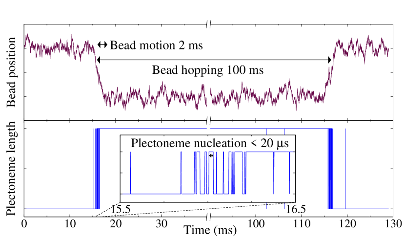
Figure 10: (Color online) Schematic illustrating relevant timescales. Since the timescale governing the bead’s motion through water (2 ms) is much slower than the plectoneme nucleation timescale (20 $\mu$s), the bead sets the experimentally measured hopping timescale (100 ms). When the bead is located at the saddle point, the free energy barrier to plectoneme formation is lowered (see Fig. 9), such that plectonemes nucleate at a rate faster than our calculated $k_{\mathrm{hopping}}$. Plectonemes have time to form and disappear many times (inset) as the bead moves slowly between the two free energy wells.

If the characteristic rate controlling the bead motion were instead made faster than the hopping rate, similar experiments could directly measure the plectoneme nucleation hopping rate. Some modifications would be relatively easy: we estimate that increasing the external force $F$ to 5.5 pN (the highest force at which plectonemes are observed in the current experiments Sheinin ) would decrease $k_{\mathrm{hopping}}$ by a factor of 3; decreasing the length of the DNA to 1 kbp would decrease $k_{\mathrm{hopping}}$ by a factor of about 2; reducing the bead’s size to 100 nm would increase $\omega_{b}$ by a factor of 2. These modifications would bring the two rates closer by about one order of magnitude. We do not see an obvious way to overcome the remaining factor of ten, but leave the challenge open to experimentalists. If this challenge can be met, future experiments may be able to directly measure the plectoneme nucleation hopping rate, giving useful information about the microscopic dynamics of DNA in water, and providing a novel testing ground for transition state theory.

Appendix A The elastic rod model

The physical properties of long DNA molecules have been found to be well-described by linear elastic theory (often referred to as the “worm-like chain” model, especially in a statistical mechanics context; see, e.g., Vologodskii and Marko (1997); Marko and Siggia (1995)). In this formulation, the DNA is modeled as a thin elastic rod, and the energy associated with deforming it from its natural relaxed state is the sum of local elastic bending, twisting, and stretching energies. The corresponding elastic constants are sensitive to experimental conditions such as the ionic concentration of the surroundings; in our experimental setup, the bend and stretch elastic constants $B$ and $S$ can be measured by fitting force-extension curves, and the (renormalized) twist elastic constant $C$ can be measured from the slope of the torque as a function of linking number. These values are listed in Table 1 Forth et al. (2008). For the low forces in the current experiment (which are in a biologically-relevant range Forth et al. (2008)), the stretch elasticity can be safely ignored ; we thus treat our DNA as an inextensible elastic rod, with energy as given in Eq. (1). Furthermore, since all parts of the DNA stay sufficiently far from touching each other in the saddle state, we also neglect nonlocal repulsive interactions (which would be required to stabilize plectonemes), allowing an analytical description of the saddle state Fain et al. (1997).

Appendix B Calculating the energy of a DNA configuration

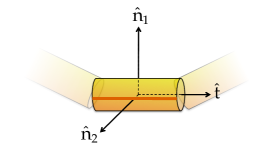
Figure 11: (Color online) Local basis vectors.

In our numerical calculations, we approximate the continuous elastic rod as a discretized chain of segments, each with fixed length $d$. The orientation of each segment is described by the rotations necessary to transform the global Cartesian axes onto the local axes of the segment. When minimizing the (free) energy, we find it convenient to use Euler angles $\phi,\theta,$ and $\psi$, since any set of Euler angles specifies a valid configuration . However, writing the energy in terms of differences of Euler angles can lead to numerical problems near the singularities at the poles. When calculating energies and forces, we therefore instead use the full rotation matrix $R$. $R$ rotates a segment lying along the $z$-axis to its final orientation; $R$’s columns are thus the two normal unit vectors followed by the tangent unit vector (see Fig. 11):

$$R^{(n)}=\left[\begin{array}[]{ccc}\hat{n}_{1}^{(n)}&\hat{n}_{2}^{(n)}&\hat{t}^{(n)}\end{array}\right]$$ (35)

$$\hat{n}_{1}=( \cos{\phi}\cos{\psi}-\cos{\theta}\sin{\phi}\sin{\psi},$$

$$- \cos{\psi}\sin{\phi}-\cos{\theta}\cos{\phi}\sin{\psi},$$

$$\sin{\theta}\sin{\psi}),$$

$$\hat{n}_{2}=( \cos{\theta}\cos{\psi}\sin{\phi}+\cos{\phi}\sin{\psi},$$ (36)

$$\cos{\theta}\cos{\phi}\cos{\psi}-\sin{\phi}\sin{\psi},$$

$$- \cos{\psi}\sin{\theta}),$$

$$\hat{t}=( \sin{\theta}\sin{\phi},-\cos{\psi}\sin{\theta},\cos{\theta}).$$

There are three degrees of freedom in the “hinge” between each segment that determine the local elastic energy: the two components of bending $\beta_{1}$ and $\beta_{2}$ (along $\hat{n}_{1}$ and $\hat{n}_{2}$, respectively), and the twist $\Gamma$. In terms of the rotation matrix

$$\Delta^{(n)}\equiv(R^{(n)})^{T}R^{(n+1)},$$ (37)

which measures the rotation between adjacent segments, mapping the $n$th segment’s axes onto those of the $(n+1)$th, the bends and twist can be written in an explicitly rotation-invariant form: to lowest order in the angles (see Section D.2),

$$\vec{\beta}\cdot\hat{n}_{1}=\beta_{1} =(\Delta_{23}-\Delta_{32})/2$$ (38)

$$\vec{\beta}\cdot\hat{n}_{2}=\beta_{2} =(\Delta_{31}-\Delta_{13})/2$$ (39)

$$\Gamma =(\Delta_{12}-\Delta_{21})/2,$$ (40)

where the $(n)$ superscripts have been omitted. The above forms are useful when the sign of a given component is necessary . Otherwise, the following squared forms may be used, which have the advantage of a larger range of validity away from zero (see Section D.2):

$$\vec{\beta}^{2} =\beta_{1}^{2}+\beta_{2}^{2}=2(1-\Delta_{33})$$ (41)

$$\Gamma^{2} =1-\Delta_{11}-\Delta_{22}+\Delta_{33}.$$ (42)

Our energy function is then the discretized version of Eq. (1):

$$E_{\mathrm{elastic}}=\frac{1}{2d}\sum_{m}B\vec{\beta}_{m}^{2}+C\Gamma_{m}^{2},$$ (43)

or, separating the bend into its two components,

$$E_{\mathrm{elastic}}=\frac{1}{2d}\sum_{m}B(\vec{\beta}_{m}\cdot\hat{n}_{1}^{(m)})^{2}+B(\vec{\beta}_{m}\cdot\hat{n}_{2}^{(m)})^{2}+C\Gamma_{m}^{2}.$$ (44)

Appendix C Transition state calculation details

C.1 Changing to the correct coordinates

So far, we have used Euler angles $(\phi,\theta,\psi)$ to parametrize the DNA configuration. We can easily calculate energy derivatives with respect to these coordinates. However, the hopping rate calculation requires that we do our path integral in the same coordinates as the dynamics, given in Section II.3, which are defined in Cartesian space with a local twist [$\vec{r}=(x,y,z,\psi)$]. To efficiently calculate the correct Hessian, then, we need to convert energy derivatives to $\vec{r}$ space.

First, we note that there is one less coordinate in Euler angle space: this comes from the inextensibility constraint, which $\vec{r}$ space does not have. Thus we add a coordinate $\Delta$ to the Euler angles specifying the length of each segment (which will usually be set to a constant $d$); we will call this set of coordinates $\vec{\alpha}=(\phi,\theta,\psi,\Delta)$. Also, $\vec{r}$ has $N+1$ elements, each defining the location of one end of a segment, while $\vec{\alpha}$ has $N$ elements, each defining the Euler angles and length of each segment. To match the number of degrees of freedom, we remove center of mass motion and set constant orientation boundary conditions by fixing the location of the first segment’s two ends and fixing the last segment’s orientation along $\hat{z}$: $\vec{r}(0)=\vec{0}$, $\vec{r}(1)=d\,\hat{z}$, $\vec{r}(N+1)=\vec{r}(N)+d\,\hat{z}$. This gives a total of $4(N-2)$ degrees of freedom.

The Jacobian we would like to calculate is

$$J_{mi,nj}=\frac{d\vec{\alpha}_{mi}}{d\vec{r}_{nj}},$$ (45)

where $m$ and $n$ label segments and $i$ and $j$ label components. First writing the Euler angles for a given segment $n$ in terms of $\vec{t}_{n}=(x,y,z)_{n+1}-(x,y,z)_{n}$,

$$\phi =\arctan{\left(-t_{y}/t_{x}\right)}$$ (46)

$$\theta =\arccos{\left(t_{z}/\sqrt{t_{x}^{2}+t_{y}^{2}+t_{z}^{2}}\right)}$$ (47)

$$\Delta =\sqrt{t_{x}^{2}+t_{y}^{2}+t_{z}^{2}}.$$ (48)

We then take derivatives with respect to Cartesian coordinates to produce the $\phi$, $\theta$, and $\Delta$ rows in the Jacobian. A subtlety arises in finding expressions for derivatives of the Euler angle $\psi$ with respect to Cartesian coordinates. We would like the derivative to correspond to rotating the adjacent segments to accommodate the change in the location of their connecting ends. Due to the way in which Euler angles are defined, this rotation does not in general leave $\psi$ unchanged, as one might naively expect. We therefore obtain the derivatives of $\psi$ by first writing the rotation matrix corresponding to infinitesimal motion in Cartesian space and then calculating the corresponding change in $\psi$. This produces the nonzero terms in the $\psi$ row of $J_{1}$ below.

In the end, we have

$$J_{mn}=\delta_{m,n}\left[J_{1}(m)+J_{2}\right]-\delta_{m,n+1}J_{1}(m),$$ (49)

where (including the names of the components for clarity)

$$\begin{array}[]{ccc}{}\hfil&{}\hfil&\begin{array}[]{cccc}\;\;\;\;\;\;\;\;x&\;\;\;\;\;y&\;\;\;\;\;\;\;\;\;\;z&\;\;\;\psi\end{array}\\ J_{1}(n)\equiv&\begin{array}[]{c}\phi\\ \theta\\ \psi\\ \Delta\end{array}&\left[\begin{array}[]{cccc}-t_{y}/p&t_{y}/p&0&0\\ t_{x}t_{z}/p\Delta^{2}&t_{y}t_{z}/p\Delta^{2}&-p/\Delta^{2}&0\\ t_{y}t_{z}/p^{2}\Delta&-t_{x}t_{z}/p^{2}\Delta&0&0\\ t_{x}/\Delta&t_{y}/\Delta&t_{z}/\Delta&0\end{array}\right],\end{array}$$ (50)

$p\equiv\sqrt{\Delta^{2}-t_{z}^{2}}$, $J_{2}\equiv\delta_{\psi,\psi}$, and all the components are evaluated at location $n$. We use this Jacobian to transform forces with respect to angles $\vec{\alpha}$ to forces with respect to $\vec{r}$, which are then used to assemble the Hessian for use in calculating the unstable mode and the entropic factors for the transition state calculation in Section II.4.

C.2 Other subtleties

Since derivatives in $\vec{r}$ space will in general couple to $\Delta$ (changing the lengths of segments), we also include an extra stretching energy:

$$E_{\mathrm{stretching}}=\frac{S}{2}\sum_{n}(\Delta_{n}-d)^{2}.$$ (51)

This avoids problems with extra zero modes corresponding to changing $\Delta$. We may choose the stretch elastic constant $S$ to match DNA (in which case it should be about 1000 pN Wang et al. (1997)); but since $S$ is so large compared to the other elastic constants, the stretching modes have much higher energy and are the same for the straight and saddle configurations, canceling in the rate equation [e.g. Eq. (21)]. Thus we find that our results are insensitive to the exact value of $S$, as expected.

As can be seen by inserting $\vec{t}=(0,0,1)$ into Eq. (50), there are singularities in the Jacobian when $\vec{t}$ points along the $z$-axis. This corresponds to the singularity in the Euler angle representation at the poles (when $\theta=0$, $\phi$ and $\psi$ are degenerate). This is a problem for our formulation because our usual boundary conditions hold the ends in the $\hat{z}$ direction. As pointed out in Ref. Kulić et al. (2007), a simple way to avoid this problem is to rotate the system away from the singularity (rotating the direction of the force as well). When performing calculations that require the Jacobian, we therefore rotate the system about the $y$-axis by an angle $\beta$ and modify the external force term in the energy from $-F\cos{\theta}$ to $-F(\cos{\beta}\cos{\theta}+\sin{\beta}\sin{\theta}\sin{\phi})$. This more general formulation also permits an explicit check that our energies and derivatives are rotation invariant.

The Hessian is constructed by taking numerical derivatives of forces, which can be calculated analytically. This gives the Hessian as a $4(N-2)\times 4(N-2)$ matrix, which is diagonalized to find eigenvalues for the entropic calculation [Eq. (21)]. At zero disorder, the zero modes must first be removed; numerically, we find that the zero modes show up conveniently as the two modes with smallest eigenvalues, a few orders of magnitude smaller than any others.

Appendix D Numerical details

D.1 Choosing $d$

As shown in Fig. 12, we must be careful to choose our discretization length (the length $d$ of each segment) such that our energy calculations are sufficiently accurate. We can check the accuracy of the discretized energy calculation by comparing with the analytical energy barrier in Eq. (8). Choosing $d=1$ nm (about 3 DNA basepairs) produces energy barriers within 0.2$kT$ of the continuum limit (corresponding to 20% changes in the hopping rate) with reasonable memory and time expenditure.

Figure 12: (Color online) Choosing $d$. Error in the discretized energy barrier [comparing to the exact result in Eq. (8)] as a function of the number of discrete segments $N$ (for $L=740$ nm and other parameters as in Table 1). Inset: the same data on a log-log plot. The green (upper) line has a slope of $-2$, showing convergence proportional to $1/N^{2}$. We choose $N=740$ ($d=1$ nm) as a good trade-off between accuracy and required computational resources.

D.2 Deriving rotation-invariant forms for bend and twist

The amount of local bend and twist can be measured by differences in the rotation matrices of adjacent segments. We would like expressions in terms of the rotation matrices that are correct to lowest order in the bend or twist angle and that are explicitly rotation invariant. Our procedure will be to form rotation invariant terms and, writing them in terms of Euler angles and their derivatives, check what they measure in terms of bend and twist.

We can first write the bend and twist in terms of derivatives of the local basis vectors (see Fig. 11) or Euler angles Fain et al. (1997):

$$\beta^{2} =\left[\dot{\vec{t}}\,\right]^{2}=\dot{\phi}^{2}\sin^{2}\theta+\dot{\theta}^{2}$$ (52)

$$\Gamma^{2} =\left[(\vec{n}\times\dot{\vec{n}})\cdot\vec{t}\,\right]^{2}=\left(\dot{\phi}\cos\theta+\dot{\psi}\right)^{2}.$$ (53)

We then form rotation-invariant terms from rotation matrices and compare their Taylor series expansions with respect to bend and twist angles to Eq. (52) and Eq. (53). First checking $\mathrm{Tr}[(R^{(n+1)}-R^{(n)})^{T}(R^{(n+1)}-R^{(n)})]$, we find that

$$\beta^{2}+\Gamma^{2} =\frac{1}{2}\left(R^{(n)}_{\alpha\beta}-R^{(n+1)}_{\alpha\beta}\right)\left(R^{(n)}_{\alpha\beta}-R^{(n+1)}_{\alpha\beta}\right)$$

$$=3-\Delta_{11}-\Delta_{22}-\Delta_{33}.$$ (54)

Next we check the dot product of the difference in the tangent unit vector $\hat{t}$:

$$\beta^{2} =\delta\hat{t}\cdot\delta\hat{t}=\left(R^{(n)}_{\alpha 3}-R^{(n+1)}_{\alpha 3}\right)\left(R^{(n)}_{\alpha 3}-R^{(n+1)}_{\alpha 3}\right)$$

$$=2(1-\Delta_{33}).$$ (55)

Eq. (54) and Eq. (55) produce Eq. (41) and Eq. (42).

To find expressions for signed $\beta$ and $\Gamma$, we notice that the above use only the diagonal elements of $\Delta$; we can also form rotation invariant terms using the off-diagonal elements, producing (with the Levi-Civita symbol $\varepsilon$)

$$\beta_{1} =\varepsilon_{1\gamma\delta}\Delta_{\gamma\delta}/2=(\Delta_{23}-\Delta_{32})/2$$ (56)

$$\beta_{2} =\varepsilon_{2\gamma\delta}\Delta_{\gamma\delta}/2=(\Delta_{31}-\Delta_{13})/2$$ (57)

$$\Gamma =\varepsilon_{3\gamma\delta}\Delta_{\gamma\delta}/2=(\Delta_{12}-\Delta_{21})/2.$$ (58)

We can see the benefit of using the squared forms [Eq. (41) and Eq. (42)] by checking their dependence on pure bending or twisting rotations. For example, with two segments differing only in twist, such that $\psi^{(n+1)}=\psi^{(n)}+\alpha$, we find that Eq. (40) and Eq. (42) produce, respectively , $\Gamma=\sin{\alpha}$ and $\Gamma^{2}=2(1-\cos\alpha)$. Plotting $\Gamma^{2}$ for the two cases (Fig. 13) demonstrates that they have the same curvature near $\alpha=0$ (by design), but using the non-squared version in Eq. (40) leads to a second minimum at $\alpha=\pi$: we find that, especially when including intrinsic bend disorder, this can cause the numerical minimizer to allow $\psi$ to slip by $\pi$ to the next minimum, unphysically removing linking number. For this reason, we use the squared forms unless otherwise necessary.

Figure 13: (Color online) Checking bend and twist expressions. (top) Two different rotation-invariant approximations to the bend or twist angle squared (green, dash-dotted; and red, dotted) compared to the actual angle squared (blue, solid). Using the non-squared version (green, dash-dotted) leads to a smaller range of validity. (bottom) Typical magnitude of bend and twist angles for a plectoneme (for $F=2$ pN, $d=1$ nm). Note that the bend and twist angles stay within the region where either approximation should be valid.

Appendix E Including intrinsic bend disorder

E.1 Setting the disorder size

As discussed in Section IV, we need to include DNA’s intrinsic bend disorder to understand the energetics of the saddle point barrier crossing. To accomplish this, we shift the zero of the elastic bend energy for each hinge; generalizing Eq. (44),

$$E_{\mathrm{bend}}=\frac{B}{2d}\sum_{m}((\vec{\beta}_{m}-\sigma_{b}\vec{\xi}_{m})\cdot\hat{n}_{1}^{(m)})^{2}+((\vec{\beta}_{m}-\sigma_{b}\vec{\xi}_{m})\cdot\hat{n}_{2}^{(m)})^{2}.$$ (59)

For each $i$, we choose each of the two components of $\xi$ from a normal distribution with unit standard deviation. We then need to relate $\sigma_{b}$ to the resulting intrinsic bend persistence length $P$. The persistence length is defined by the decay of orientation correlations:

$$\langle\hat{t}(0)\cdot\hat{t}(s)\rangle=\langle\cos\theta(s)\rangle=e^{-s/P},$$ (60)

where $\theta(s)$ is the angle between segments separated by arclength $s$ Bednar et al. (1995). For small $s$ [and thus small $\theta(s)$], Eq. (60) becomes

$$1-\frac{1}{2}\langle\theta(s)^{2}\rangle=1-\frac{s}{P}.$$ (61)

At zero temperature and zero force, the size of $\langle\theta(s)^{2}\rangle$ is set by the intrinsic bends $\xi_{m}$ only; we are doing a random walk in two dimensions with one step of root-mean-square size $\sqrt{2}\sigma_{b}$ taken for every segment of length $d$. Thus $\langle\theta(s)^{2}\rangle=2\frac{s}{d}\sigma_{b}^{2}$, which when inserted into Eq. (61) gives the desired relation between persistence length $P$ and the size of individual random bends $\sigma_{b}$:

$$P=\frac{d}{\sigma_{b}^{2}}.$$ (62)

We will also define a convenient parameter $D$ controlling disorder strength that is independent of the segment length $d$:

$$D\equiv\frac{\sigma_{b}}{\sqrt{d}},$$ (63)

such that

$$P=D^{-2}.$$ (64)

E.2 First order changes in the energy barrier due to disorder

Figure 14: (Color online) Typical sensitivity of saddle energy to bending disorder strength as a function of position [$A(s)$, as defined in Eq. (67)], for $L=740$ nm. Peaks indicate positions where plectoneme nucleation is energetically favored. For DNA, the bending disorder strength $D$ is estimated to be of order 0.01 to 0.1 nm^-1/2; thus we expect pinning to individual sites (with barriers on the order of $kT$), but also that multiple plectoneme locations will contribute to the final hopping rate in Eq. (32) (with multiple locations having energy within about 1 $kT$).

Figure 15: (Color online) The lowest saddle energy as a function of disorder strength $D$. The blue dots are the true saddle energies, calculated by numerically zeroing forces on the saddle configuration. The green line represents the first-order approximation given by $DA(s^{*})$; we see that the approximation correctly predicts the scale of the change, but overestimates it by many $kT$ at large disorder.

How does disorder change the energy of the saddle point? Since the disorder changes only the bending energy, we can find the lowest order change from the zero disorder energy by taking the derivative of Eq. (59) with respect to disorder strength $\sigma_{b}$ at $\sigma_{b}=0$:

$$\frac{dE}{d\sigma_{b}}\bigg{|}_{\sigma_{b}=0} =\frac{dE_{\mathrm{bend}}}{d\sigma_{b}}\bigg{|}_{\sigma_{b}=0}$$

$$=-\frac{B}{d}\sum_{m}(\vec{\beta}_{m}\cdot\hat{n}_{1}^{(m)})(\vec{\xi}_{m}\cdot\hat{n}_{1}^{(m)})$$

$$\quad\quad\quad\>\>\>+(\vec{\beta}_{m}\cdot\hat{n}_{2}^{(m)})(\vec{\xi}_{m}\cdot\hat{n}_{2}^{(m)})$$

$$=-\frac{B}{d}\sum_{m}\vec{\beta}_{m}\cdot\vec{\xi}_{m},$$ (65)

or, in terms of disorder strength $D$ defined in Eq. (63),

$$\frac{dE}{dD}\bigg{|}_{D=0}=-\frac{B}{\sqrt{d}}\sum_{m}\vec{\beta}_{m}\cdot\vec{\xi}_{m}.$$ (66)

We will specifically be interested in the derivative of the saddle configuration’s energy, which will depend on its location $s$ and rotation $\rho$. Noting that $\rho$ will simply rotate the bend vector $\vec{\beta}$, we can write down the form of the dependence on $\rho$:

$$E_{\mathrm{saddle}}^{{}^{\prime}}(s,\rho)\equiv\frac{dE_{\mathrm{saddle}}(s,\rho)}{dD}\bigg{|}_{D=0}=-A(s)\cos(\rho-\rho^{*}(s))$$ (67)

for some $A(s)$ and $\rho^{*}(s)$. $A(s)$ gives the maximum derivative (sensitivity to disorder) at position $s$, and $\rho^{*}(s)$ is the preferred rotation of the saddle that gives the maximum (negative) derivative. We can find $A(s)$ and $\rho^{*}(s)$ numerically using the derivative calculated at two values of $\rho$ separated by $\pi/2$:

$$A(s) =\sqrt{\left(E_{\mathrm{saddle}}^{{}^{\prime}}(s,0)\right)^{2}+\left(E_{\mathrm{saddle}}^{{}^{\prime}}(s,\pi/2)\right)^{2}}$$ (68)

$$\rho^{*}(s) =\arctan\left(\frac{E_{\mathrm{saddle}}^{{}^{\prime}}(s,\pi/2)}{E_{\mathrm{saddle}}^{{}^{\prime}}(s,0)}\right).$$ (69)

Fig. 14 shows a typical $A$ as a function of $s$. Fig. 15 compares the first-order approximation to the saddle energy at the location $s^{*}$, given by $DA(s^{*})$, to $E_{\mathrm{saddle}}$ calculated numerically by zeroing forces (see Section E.3). We see that the approximation correctly predicts the scale of the change for the disorder sizes in which we are interested, but overestimates the change by many $kT$ for large disorder. We therefore use the first-order approximation to find the likely locations of the lowest energy saddle points [at the peaks of $A(s)$], and then zero the forces numerically.

To estimate the typical size of this sensitivity to disorder, we first note that the bend magnitude for the saddle configuration is [inserting Eqs. (5) into Eq. (52)]

$$|\vec{\beta}_{\mathrm{saddle}}|=\frac{2d}{\ell}{\text{sech}}{\left(\frac{s}{\ell}\right)}.$$ (70)

Approximating the function ${\text{sech}}{(x)}$ as 1 in the range $-2<x<2$ and 0 elsewhere, Eq. (66) becomes

$$\frac{dE_{\mathrm{saddle}}}{dD}\bigg{|}_{D=0}\approx-\frac{B}{\sqrt{d}}\frac{2d}{\ell}\sum_{n=0}^{4\ell/d}\xi_{m}$$ (71)

for randomly distributed $\xi$ with unit variance, which produces

$$\sqrt{\big{\langle}\big{(}\frac{dE_{\mathrm{saddle}}}{dD}\big{)}^{2}\big{\rangle}}\approx\frac{4B}{\sqrt{\ell}}.$$ (72)

Inserting $B=(43$ nm$)kT$ and $\ell\approx 10$ nm gives a typical sensitivity of about $(50$ nm${}^{1/2})kT$, agreeing with the scale found in the full calculation, as shown in Fig. 14.

E.3 Finding saddle points

With large disorder, the saddle points must be found numerically. We start by estimating the set of saddle locations $\{s^{*}\}$ and rotations $\{\rho^{*}\}$ using first order perturbation theory (Section E.2). We find the local maxima of $A(s)$ using a one-dimensional local search method starting from a set of points spaced by the saddle configuration length scale $\ell$. This gives $\{s^{*}\}$, from which $\{\rho^{*}\}$ can be found using Eq. (69). For each $s^{*}$ and corresponding $\rho^{*}$, we create a zero-disorder saddle configuration [Eqs. (5)], and then use this as the starting point for a multidimensional equation solver (scipy.fsolve) that numerically locates the saddle with disorder by finding solutions with zero net force on each segment.

References

- Forth et al. (2008) S. Forth, C. Deufel, M. Y. Sheinin, B. Daniels, J. P. Sethna, and M. D. Wang, Phys. Rev. Lett. 100, 148301 (2008).
- Brutzer et al. (2010) H. Brutzer, N. Luzzietti, D. Klaue, and R. Seidel, Biophys. J. 98, 1267 (2010).
- Bednar et al. (1995) J. Bednar, P. Furrer, V. Katritch, A. Z. Stasiak, J. Dubochet, and A. Stasiak, J. Mol. Biol. 254, 579 (1995).
- Trifonov et al. (1987) E. N. Trifonov, R. K.-Z. Tan, and S. C. Harvey, in DNA Bending and Curvature, edited by W. K. Olson, M. H. Sarma, and M. Sundaralingam (Adenine Press, 1987), pp. 243–254.
- Nelson (1998) P. Nelson, Phys. Rev. Lett. 80, 5810 (1998).
- Vologodskaia and Vologodskii (2002) M. Vologodskaia and A. Vologodskii, J. Mol. Biol. 317, 205 (2002).
- Langer (1968) J. S. Langer, Phys. Rev. Lett. 21, 973 (1968).
- Langer (1969) J. S. Langer, Ann. Phys. 54, 258 (1969).
- Hänggi et al. (1990) P. Hänggi, P. Talkner, and M. Borkovec, Rev. Mod. Phys. 62, 251 (1990).
- Coleman (1977) S. Coleman, in Proc. Int. School of Subnuclear Physics (Erice, 1977), p. 265.
- Langer and Ambegokar (1967) J. S. Langer and V. Ambegokar, Phys. Rev. 164, 498 (1967).
- McCumber and Halperin (1970) D. E. McCumber and B. I. Halperin, Phys. Rev. B 1, 1054 (1970).
- Fain et al. (1997) B. Fain, J. Rudnick, and S. Östlund, Phys. Rev. E 55, 7364 (1997).
- Balaeff et al. (2004) A. Balaeff, C. R. Koudella, L. Mahadevan, and K. Schulten, Phil. Trans. R. Soc. Lond. A 362, 1355 (2004).
- Cox (1970) R. G. Cox, J. Fluid Mech. 44, 791 (1970).
- Klenin et al. (1998) K. Klenin, H. Merlitz, and J. Langowski, Biophys. J. 74, 780 (1998).
- Mülhardt (2006) C. Mülhardt, Molecular Biology and Genomics (Academic Press, 2006).
- Daniels et al. (2009) B. C. Daniels, S. Forth, M. Y. Sheinin, M. D. Wang, and J. P. Sethna, Phys. Rev. E 80, 040901(R) (2009).
- Wang et al. (1997) M. D. Wang, H. Yin, R. Landick, J. Gelles, and S. M. Block, Biophys. J. 72, 1335 (1997).
- (20) M. Sheinin, personal communication.
- Vologodskii and Marko (1997) A. V. Vologodskii and J. F. Marko, Biophys. J. 73, 123 (1997).
- Marko and Siggia (1995) J. F. Marko and E. D. Siggia, Macromolecules 28, 8759 (1995).
- Kulić et al. (2007) I. M. Kulić, H. Mohrbach, R. Thaokar, and H. Schiessel, Phys. Rev. E 75, 011913 (2007).
- Crut et al. (2007) A. Crut, D. A. Koster, R. Seidel, C. H. Wiggins, and N. H. Dekker, Proc. Natl. Acad. Sci. USA 104, 11957 (2007).
- Doyle and Underhill (2005) P. S. Doyle and P. T. Underhill, in Handbook of Materials Modeling, edited by S. Yip (Springer, 2005), p. 2619.
- Rotne and Prager (1969) J. Rotne and S. Prager, J. Chem. Phys. 50, 4831 (1969).