The Molecular Outflows in the $\rho$ Ophiuchi Main Cloud:
Implications For Turbulence Generation

Abstract

We present the results of CO ($J=3-2$) and CO ($J=1-0$) mapping observations toward the active cluster forming clump, L1688, in the $\rho$ Ophiuchi molecular cloud. From the CO ($J=3-2$) and CO ($J=1-0$) data cubes, we identify five outflows, whose driving sources are VLA 1623, EL 32, LFAM 26, EL 29, and IRS 44. Among the identified outflows, the most luminous outflow is the one from the prototypical Class 0 source, VLA 1623. We also discover that the EL 32 outflow located in the Oph B2 region has very extended blueshifted and redshifted lobes with wide opening angles. This outflow is most massive and have the largest momentum among the identified outflows in the CO ($J=1-0$) map. We estimate the total energy injection rate due to the molecular outflows identified by the present and previous studies to be about 0.2 $L_{\odot}$, larger than or at least comparable to the turbulence dissipation rate [$\approx(0.03-0.1)L_{\odot}$]. Therefore, we conclude that the protostellar outflows are likely to play a significant role in replenishing the supersonic turbulence in this clump.

1 Introduction

It is now well accepted that the majority of stars in our Galaxy form in clusters (Lada & Lada, 2003). Recent observations have revealed that active cluster forming regions are not distributed uniformly in parent molecular clouds, but localized and embedded in dense clumps with typical sizes of $\sim$ 1 pc and masses of $10^{2}\sim$ 10${}^{3}M_{\odot}$ (e.g., Ridge et al., 2003). More than half of all the young stellar populations associated with a parent molecular cloud are confined in such pc-scale, cluster forming clumps (e.g., Lada et al., 1991; Carpenter, 2000; Allen et al., 2006), where many stars at different stages of formation are born in close proximity to one another. For example, in the Perseus molecular cloud, one of the nearby well-studied star forming regions, two pc-scale cluster forming clumps, IC 348 and NGC 1333, contain about 80% of the young stars associated with this cloud (Carpenter, 2000). The mass fraction of molecular gas occupied by these two regions in the parent molecular cloud is less than a few tens %. In such dense clumps, the feedback from the older generation of stars affects the formation of the younger generation of stars (e.g., Norman & Silk, 1980; McKee, 1989; Vazquez-Semadeni et al., 2010).

Among the stellar feedback processes, protostellar outflows have been considered to be one of the important mechanisms to control the structure and dynamical properties of cluster forming clumps (Bally et al., 1996; Shu et al., 2000; Matzner & McKee, 2000; Matzner, 2007) because the outflows from a group of young stars interact with a substantial volume of their parent clump by sweeping up the gas into shells. Indeed, recent numerical simulations of cluster formation have demonstrated that the protostellar outflows largely regulate the structure formation and star formation in a dense cluster forming clump (Li & Nakamura, 2006; Nakamura & Li, 2007; Wang et al., 2010; Li et al., 2010). Li & Nakamura (2006) showed that the supersonic turbulence in dense clumps can be maintained by the momentum injection from the protostellar outflows (see also Carroll et al., 2009), and thus the clumps as a whole can be supported by the turbulent pressure due to the protostellar outflows against global gravitational collapse at least for several dynamical times. Furthermore, Nakamura & Li (2007) showed that the global star formation efficiency tends to be reduced by the momentum injection from the protostellar outflows, although local star formation can often be triggered by the dynamical compression due to the protostellar outflows. These studies indicate that the protostellar outflow feedback is a key to understanding the formation of stars in a pc-scale cluster forming clump.

Recent millimeter and submillimeter observations of nearby pc-scale cluster forming clumps have revealed the significant role of protostellar outflows in clustered star formation. An excellent example is NGC 1333, where several protostellar outflows apparently overlapping and interacting with themselves are found in the central region of the dense clump; those outflows influence the distribution of the dense gas significantly (Sandell & Knee, 2001; Gutermuth et al., 2009). The less dense parts, seen as cavities, are found to be filled with high-velocity gas created by the outflows (Knee & Sandell, 2000; Walsh et al., 2007; Hatchell et al., 2007; Hatchell & Dunham, 2009). On the basis of the ¹³CO ($J=1-0$) observations, Quillen et al. (2005) found 22 cavities with sizes of 0.1 $-$ 0.2 pc in diameter in the central region of NGC 1333 (see also Cunningham et al., 2006). Those cavities appear to expand slowly. They interpreted those cavities as remnants of past YSO outflow activity, although the role of those “fossil” cavities in cloud dynamics is still unclear.

Another example is the Serpens clump, where several powerful outflows were identified by the CO ($J=2-1$) observations (Davis et al., 1999). The energy injection rate of these outflows is comparable to or somewhat larger than the dissipation rate of the turbulent energy in this clump, indicating that the outflows are the main source of the supersonic turbulence (Sugitani et al., 2010). Sugitani et al. (2010) suggested that the outflows in this clump have enough momentum to support the whole clump against global collapse. For NGC 2264-C, Maury et al. (2009) suggested that the parent clump cannot be sufficiently supported by the outflows in the current generation, although they are likely to contribute much to maintaining the observed turbulence. In the Orion Molecular Cloud-2 FIR 3/4 region, Shimajiri et al. (2008) found an observational example showing that the dynamical interaction of protostellar outflows with a dense clump may have triggered fragmentation of the clump, leading to future star formation. In this paper, to gain further evidence of the significant role of protostellar outflows in clustered star formation, we investigate the outflow activity in the dense part of the $\rho$ Ophiuchi molecular cloud (hereafter the $\rho$ Ophiuchi main cloud), one of the nearby pc-scale cluster forming clumps, on the basis of CO ($J=3-2$) and CO ($J=1-0$) observations.

The $\rho$ Ophiuchi main cloud is a suitable object to investigate the star formation process in a cluster forming clump because this cloud is the nearest pc-scale cluster forming clump at a distance of about 125 pc (e.g., Lombardi et al. 2008; Loinard et al. 2008; Wilking et al. 2008). The $\rho$ Oph clump is known to harbor a rich cluster of young stellar objects (YSOs) in different evolutionary stages (Wilking et al. 2008; Enoch et al. 2008; Jørgensen et al. 2008). On the basis of the recent infrared observations using the Spitzer space telescope, Padgett et al. (2008) identified about 300 YSOs, including Class 0/I/II/III sources, most of which are associated with the central region of the $\rho$ Ophiuchi main cloud. Furthermore, recent millimeter and submillimeter dust continuum observations of $\rho$ Oph have revealed that a large number of dense cores are concentrated in the central dense part of the clump and their mass spectra are similar in shape to the stellar IMF (Motte et al., 1998; Johnstone et al., 2000; Stanke et al., 2006). These facts indicate that active star formation is still ongoing in this cloud.

So far, more than 10 molecular outflows from the YSOs have been identified in $\rho$ Oph (e.g., Bontemps et al., 1996; Sekimoto et al., 1997; Kamazaki et al., 2003; Wilking et al., 2008). The most spectacular outflow in $\rho$ Oph is the one from a prototypical Class 0 source, VLA 1623, (André et al., 1990; Dent et al., 1995), which is associated with Herbig-Haro objects, many knots of the H₂ emission at 2.12 $\mu$m, and the water masers. Dent et al. (1995) mapped the molecular outflow from the VLA 1623 using CO$(J=3-2)$ emission. They revealed that the outflow is highly-collimated with an opening angle less than 1.6 degree, extending over a length of about 0.5 pc. Kamazaki et al. (2003) discovered three other molecular outflows in the Oph A and B2 regions, although they did not successfully map the entire outflow lobes. In the southern part of $\rho$ Oph, Bussmann et al. (2007) mapped the outflows from EL 29 and LFAM 26. These outflows appear to be less powerful than the VLA 1623 outflow. However, the physical properties of the molecular outflows previously identified have not been well determined because of the lack of the large-scale mapping observations. To study how the outflows affect the clump dynamics and local star formation, we have performed the CO ($J=3-2$) and CO ($J=1-0$) observations toward the $\rho$ Oph main cloud, using the ASTE 10 m and Nobeyama 45 m telescopes, respectively, and have derived the physical properties of the outflows identified in the clump.

The rest of the paper is organized as follows. First, we present the details of our CO $(J=3-2)$ and CO $(J=1-0)$ mapping observations in Section 2. In Section 3, we derive the physical parameters of the molecular outflows identified from our CO ($J=3-2$) and CO ($J=1-0$) maps. Then, we make a brief discussion of how the observed outflows interact with the dense cores identified from the H¹³CO⁺ ($J=1-0$) map by Maruta et al. (2010) in Section 4. We also estimate how the observed outflows contribute to turbulence generation in this clump, and compare the clump with other nearby cluster forming clumps, Serpens and NGC 1333. Finally, we summarize our main conclusion in Section 5.

2 Observations

2.1 CO ($J=3-2$) Observations

The CO ($J=3-2$; 345.7959899GHz) mapping observations were carried out with the ASTE 10 m telescope (Ezawa et al., 2004) during the period of 2004 October. The beamsize in HPBW of the ASTE telescope is 22^′′, which corresponds to 0.013 pc at a distance of 125 pc. The main-beam efficiency, $\eta_{\rm 32}$, was 0.35 at 345 GHz. We used a 345 GHz SIS heterodyne receiver, which had the typical system noise temperature of 175-350 K in DSB mode at the observed elevation. The temperature scale was determined by the chopper-wheel method, which provides us with the antenna temperature, $T_{A}^{*}$, corrected for the atmospheric attenuation. As a backend, we used four sets of 1024 channel autocorrelators, providing us with a frequency resolution of 125 kHz that corresponds to 0.11 km s^-1 at 345 GHz. The position switching technique was employed to cover the dense region of the $\rho$ Ophiuchi main cloud, about $23^{\prime}\times 23^{\prime}$ area, corresponding to about 0.8 pc $\times$ 0.8 pc at a distance of 125 pc. After subtracting linear baselines, the data were convolved with a Gaussian-tapered Bessel function (Magnum et al. 2007) and were resampled onto a 5^′′ grid. The resultant effective FWHM resolution is 40^′′. The typical rms noise level is 0.28 K in brightness temperature ($T_{\rm mb}$) with a velocity resolution of 0.4 km s^-1.

2.2 CO ($J=1-0$) Observations

As shown in the next section, our CO ($J=3-2$) observations revealed that the outflow previously identified by Kamazaki et al. (2003) in the Oph B2 region, the EL 32 outflow, is very extended. Unfortunately, the CO ($J=3-2$) map does not cover the whole redshifted outflow lobe. To map the whole extent of the EL 32 outflow, we performed the CO ($J=1-0$) observations using the Nobeyama 45 m radio telescope. The CO ($J=1-0$; 115.2712018 GHz) mapping observations were carried out with the 25-element focal plane receiver BEARS equipped in the Nobeyama 45 m telescope during the period from December 2009 to May 2010, as a part of the Nobeyama 45m Legacy Project (see http://www.nro.nao.ac.jp/). At 115 GHz, the telescope has a FWHM beam size of 15^′′ and a main beam efficiency, $\eta_{10}$, of 0.32. At the back end, we used 25 sets of 1024 channel auto-correlators (ACs) which have bandwidths of 32 MHz and frequency resolutions of 37.8 kHz (Sorai et al., 2000). The frequency resolution corresponds to a velocity resolution of 0.1 km s^-1 at 115 GHz. During the observations, the system noise temperatures were in the range between 300 to 900 K in DSB at the observed elevation. The standard chopper wheel method was used to convert the output signal into the antenna temperatures ($T_{A}^{*}$), corrected for the atmospheric attenuation. Our mapping observations were made by the OTF mapping technique (Sawada et al., 2008). We adopted a spheroidal function as a gridding convolution function (GCF) to calculate the intensity at each grid point of the final cube data with a spatial grid size of 12^′′. The final effective resolution of the map is 30^′′. The rms noise level of the final map is 1.0 K in brightness temperature ($T_{\rm mb}$) at a velocity resolution of 0.4 km s^-1.

3 Results

3.1 CO ($J=3-2$) and CO ($J=1-0$) maps

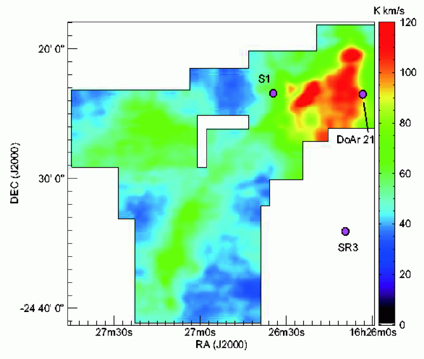
Figure 1: CO ($J=3-2$) total integrated intensity map in the velocity range from $v_{\rm LSR}=-9.8$ km s^-1 to +12.2 km s^-1 toward the $\rho$ Ophiuchi main cloud. The CO ($J=3-2$) integrated intensity is shown in color in units of K km s^-1. The circles indicate the positions of B stars S1, DoAr 21, and SR3.

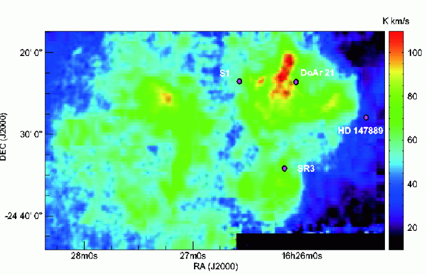
Figure 2: CO ($J=1-0$) total integrated intensity map in the velocity range from $v_{\rm LSR}=-3.2$ km s^-1 to +8.0 km s^-1 toward the $\rho$ Ophiuchi main cloud. The CO ($J=1-0$) integrated intensity is shown in color in units of K km s^-1. The circles indicate the positions of B stars S1, SR3, DoAr 21, and HD 147889.

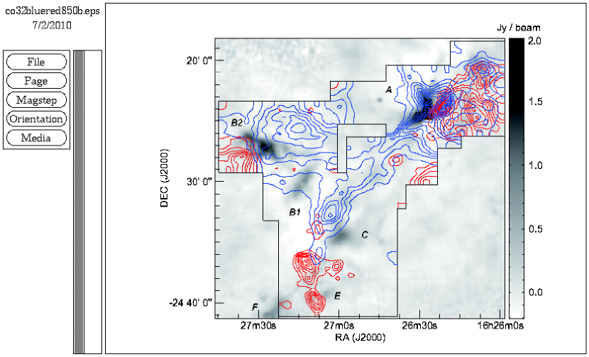
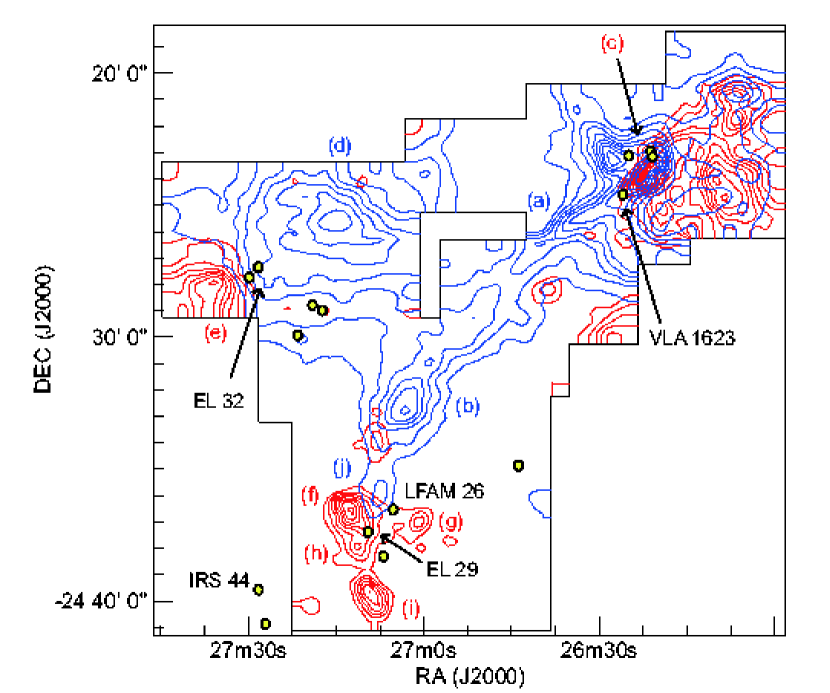
Figure 3: (a) CO ($J=3-2$) map of the $\rho$ Ophiuchi main cloud on the 850 $\mu$m image obtained by Johnstone et al. (2000). Blue contours represent blueshifted CO ($J=3-2$) intensity integrated between $-9.8$ km s^-1 and 2.2 km s^-1, starting from 18 K km s^-1 at intervals of 4 K km s^-1. Red contours represent redshifted CO ($J=3-2$) intensity integrated between $7.4$ km s^-1 and 11.8 km s^-1, starting from 1.6 K km s^-1 at intervals of 0.8 K km s^-1. The gray scale shows the 850 $\mu$m image in units of $Jy/{\rm beam}$. The dense subclumps are designated by A, b1, B2, C, E, and F. (b) CO ($J=3-2$) map of the $\rho$ Ophiuchi main cloud overlaid with the positions of the embedded YSOs listed by van Kempen et al. (2009) and some other YSOs with the yellow circles. Positions of several peaks of outflow components detected by the CO ($J=3-2$) observations are indicated by the alphabets (a) through (j).

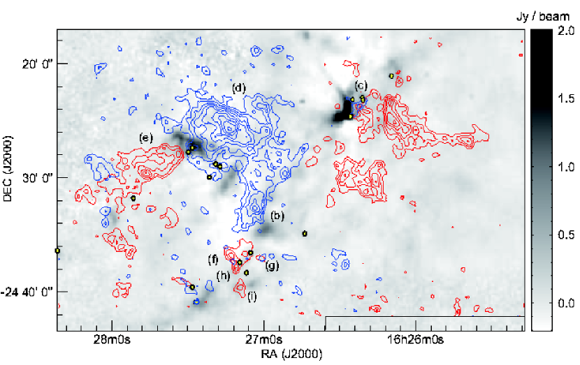
Figure 4: CO ($J=1-0$) map of the $\rho$ Ophiuchi main cloud on the 850 $\mu$m image obtained by Johnstone et al. (2000). Blue contours show the CO ($J=1-0$) intensity integrated between $-4.0$ km s^-1 and 1.2 km s^-1, starting from 8.9 K km s^-1 at intervals of4.1 K km s^-1. Red contours show the CO ($J=1-0$) intensity integrated between 6.4 km s^-1 and 9.2 km s^-1, starting from 4.1 K km s^-1 at intervals of 2.8 K km s^-1. The gray scale, symbols, and alphabets are the same as those of Figure 3.

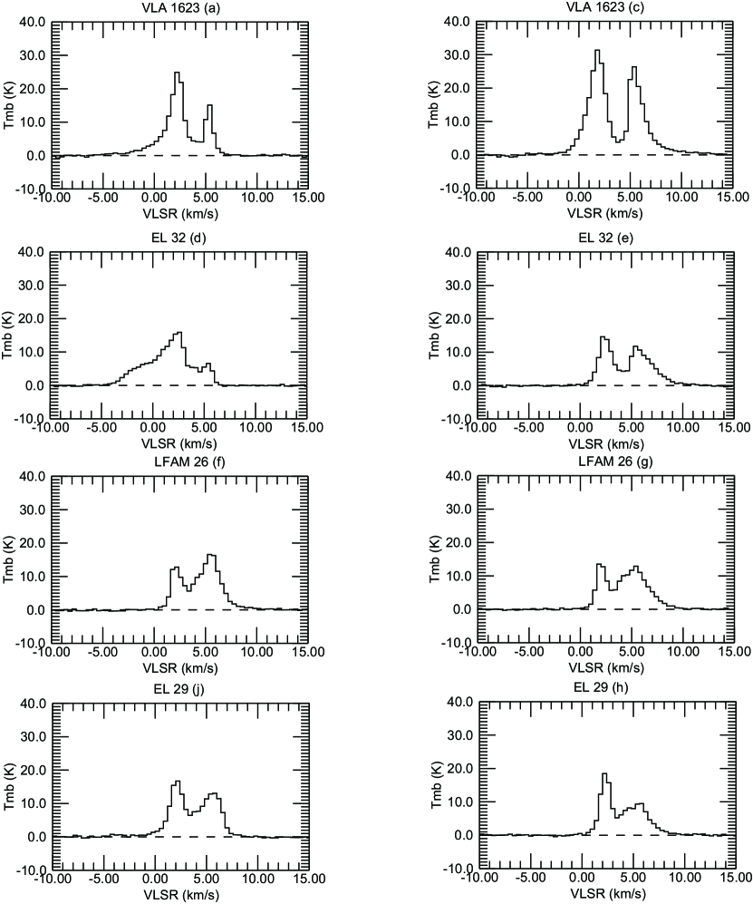
Figure 5: CO ($J=3-2$) spectra toward several high-velocity lobes indicated by alphabets in Figure 3. Each spectra is smoothed in a $1^{\prime}\times 1^{\prime}$ grid centered at the position of the peak intensity.

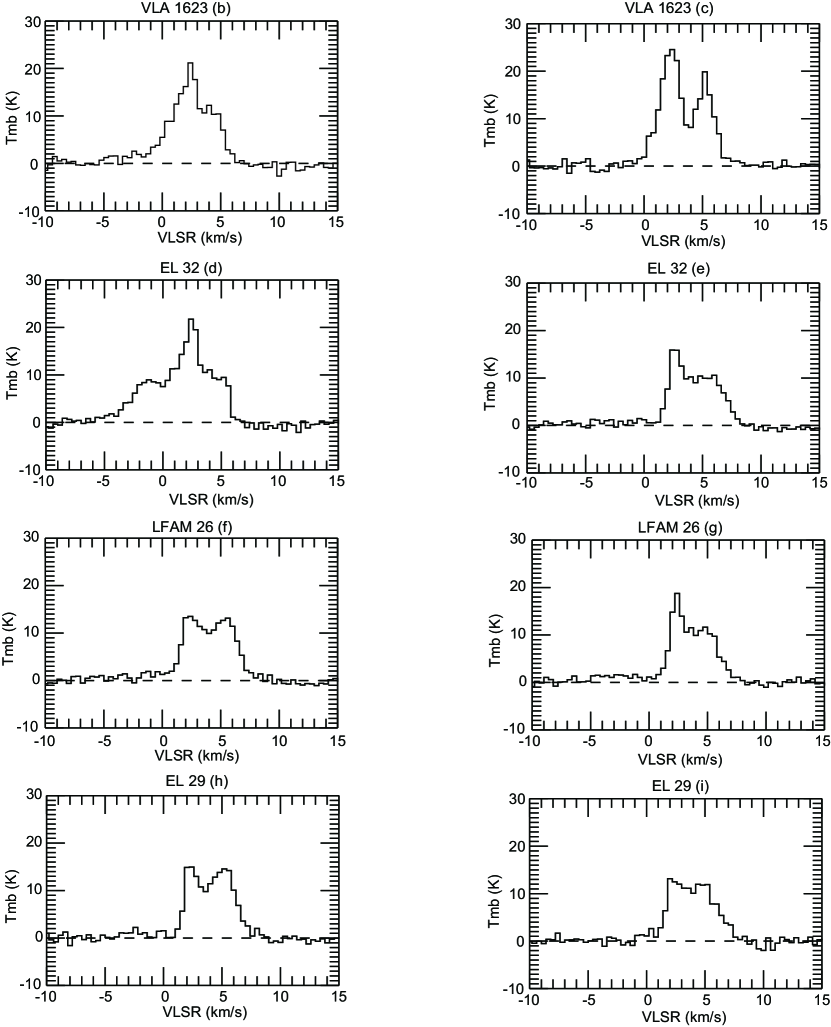
Figure 6: CO ($J=1-0$) spectra toward several high-velocity lobes indicated by alphabets in Figure 4. Each spectra is smoothed in a $1^{\prime}\times 1^{\prime}$ grid centered at the position of the peak intensity.

In Figures 1 and 2, we present the CO ($J=3-2$) and CO ($J=1-0$) integrated intensity maps in the ranges of $v_{\rm LSR}=-9.8\sim+12.2$ km s^-1 and $v_{\rm LSR}=-3.2\sim+8.0$ km s^-1, respectively. In Figures 3 and 4, the distributions of the blueshifted and redshifted CO ($J=3-2$) and CO ($J=1-0$) components, respectively, are also shown on the 850$\mu$m images obtained by Johnstone et al. (2000). In Figure 3a, several dense subclumps, which are recognized in the 850 $\mu$m images, are designated by A, B1, B2, C, D, E, and F. By comparing the H¹³CO⁺ spectra with the ¹²CO ($J=3-2$ and $J=1-0$) ones at the same position, the shapes of the ¹²CO ($J=3-2$) and ¹²CO ($J=1-0$) line profiles appear to be caused mainly by self-absorption rather than multiple velocity components (see also Figures 5 and 6).

The CO $(J=1-0)$ map in Figure 2 shows a clear break between the east and west parts of the $\rho$ Oph clump, although the radial velocities of the two parts are not so different ($v_{\rm LSR}\sim 3.5-4.5$ km s^-1). The CO $(J=3-2)$ integrated intensity map also appears to reasonably follow that of CO $(J=1-0)$, although the detailed distributions are different. The strongest CO ($J=3-2$) emission comes from the western side of Oph A (see Figure 1). As shown later, the region with the strongest CO ($J=3-2$) emission has both the blueshifted and redshifted components that are likely to be due to the outflow from the VLA 1623 source. In the entire Oph A filament, the CO ($J=3-2$) component blueshifted from the systemic velocity of Oph A is predominantly strong, suggesting that Oph A is compressed from the far side by the photodissociation region (PDR) excited by a young B3 star, S1.

The second strongest CO ($J=3-2$) emission comes near the north-west edge of the observational box, in which the CO ($J=1-0$) integrated intensity is the strongest. This region has both broadly distributed blueshifted and redshifted components, and may be influenced by the PDR excited by the B2 star, HD 147889. There are two other areas having moderately strong CO ($J=3-2$) emission. One is located near the north-east part of the CO ($J=3-2$) observational box, and the other is an elongated structure running from the box center to the south-east part. As discussed below, these two components originate from the high velocity gas by molecular outflows.

3.2 Outflow Identification

Using the CO ($J=3-2$) and CO ($J=1-0$) data cubes, we identified molecular outflows as follows (e.g., Takahashi et al., 2008). First, we scrutinized the velocity channel maps of both the data to find localized blueshifted or redshifted emission in the area within a radius of 1^′ from each YSO. Here, we used the YSO list obtained by Jørgensen et al. (2008) and van Kempen et al. (2009). From our CO ($J=3-2$) data, we identified 4 outflows. All these outflows can also be clearly recognized in the CO $(J=1-0)$ map. In addition, we identified one outflow from the CO ($J=1-0$) data, which is located outside our CO ($J=3-2$) map. All the outflows identified in the present paper were already detected by previous studies. The characteristics of the identified outflows are summarized in Table 1. In Figures 5 and 6, we present the CO ($J=3-2$) and CO ($J=1-0$) spectra centered on some of the high-velocity lobes, respectively. Each of the spectra shows signs of significant self-absorption due to the ambient gas at ambient velocities; both the CO line emission is clearly optically thick. In the following, we discuss the characteristics of the outflows identified in the present paper, and then derive their physical parameters.

3.3 Individual Outflows

3.3.1 VLA 1623

In Figure 3, two highly-collimated, strong blueshifted-components labeled (a) and (b) can be clearly recognized. They trace the collimated (south-east) outflow from the VLA 1623 source, which was first discovered by André et al. (1990) with the CO ($J=2-1$) observations. The north-west lobe of this outflow, labeled (c), is less prominent than the south-east one. The north-west flow has the low-velocity blue and redshifted components, suggesting that the outflow axis is almost parallel to the plane of the sky. This is in good agreement with the CO ($J=2-1$) observations of André et al. (1990). However, as shown in the next subsection, some physical quantities of the outflow are significantly different from theirs. This is due to the fact that their observations did not cover the whole VLA 1623 outflow. For example, our outflow size is larger by a factor of 5, the outflow velocity is smaller by a factor of 2, and thus the estimated dynamical time of the south-east component is longer by a factor of about 10 than that estimated by André et al. (1990). When the outflow parameters are estimated using the same area as they mapped, our quantities agree reasonably with those derived by André et al. (1990).

The whole outflow lobes [the components (a), (b), and (c)] were first mapped by Dent et al. (1995) using the CO $(J=3-2)$ observations. They found that the blueshifted flow is extended over a length of about 0.5 pc with a narrow opening angle of less than 1.6 degree. Our CO ($J=3-2$) map is in good agreement with that of Dent et al. (1995). Since this component is distinct in our CO $(J=1-0)$ map presented in Figure 4, we think that it can be detected with the CO ($J=2-1$) emission. Our total mass and momentum of the outflow are reasonably in good agreement with those of Dent et al. (1995), taking into account the different adopted fractional abundance ratio and distance to $\rho$ Oph, which cause the difference in the mass estimation by a factor of 3. The blueshifted components are also remarkable in the line profiles presented in Figures 5 and 6, in which the line profiles of the components (a) and (b) show strong blueshifted wings.

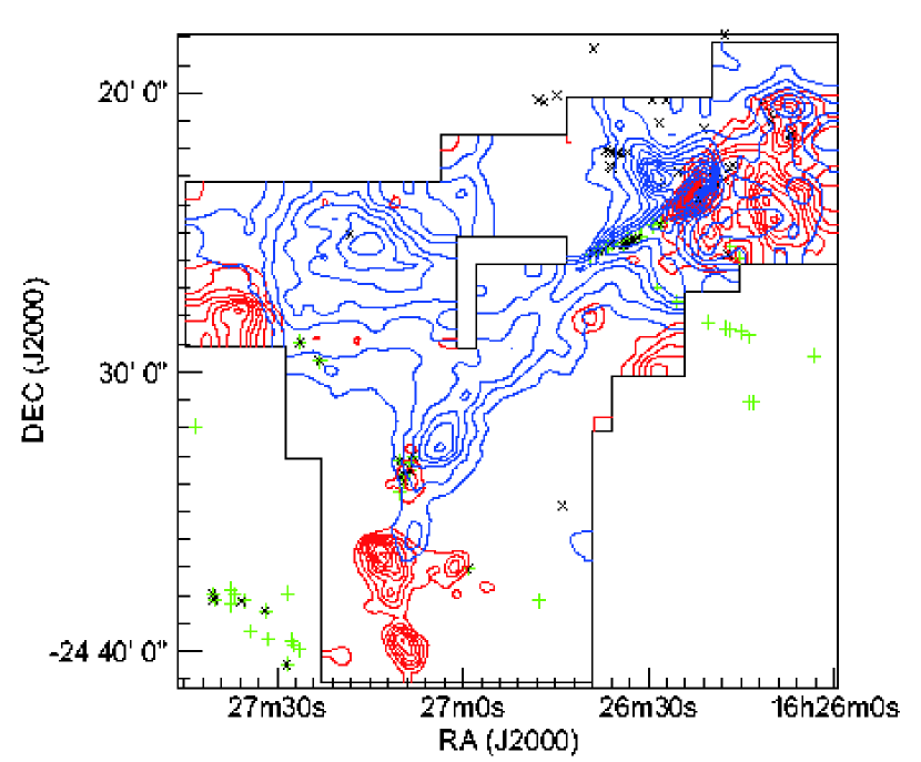
Figure 7: CO ($J=3-2$) map of the $\rho$ Ophiuchi main cloud. The contours are the same as those of Figure 3. The crosses and pluses indicate the positions of the H₂ knots identified by Gómez et al. (2003) and Khanzadyan et al. (2004), respectively.

In Figure 7, we show the positions of the H₂ knots identified by Gómez et al. (2003) and Khanzadyan et al. (2004). Many H₂ knots are associated with the blueshifted lobe labeled (a) in Figure 3b. These H₂ knots are clearly recognized in the IRAC channel 2 (4.5$\mu$m) image taken by the Spitzer space telescope (Zhang & Wang, 2010). Khanzadyan et al. (2004) compared their H₂ knots with those identified by Gómez et al. (2003) to measure the proper motions of the H₂ knots, and estimated the flow speed of about 130 km s^-1, which is much faster than the outflow speed of about 20 km s^-1 estimated from our CO ($J=3-2$) data.

3.3.2 Elias 32 and IRS 44

In our CO ($J=3-2$) image shown in Figure 3, we can clearly recognize a spatially extended outflow in the Oph B2 region (labeled (d) and (e)). The line profiles presented in Figures 5 and 6 also show distinct high-velocity wing emission for both the blueshifted and redshifted components. In particular, the blueshifted wings of both the CO ($J=3-2$) and CO ($J=1-0$) line profiles are very strong. This outflow appears to be from a Class I YSO, Elias 32, as suggested by Kamazaki et al. (2003). Although in our CO ($J=3-2$) image, most of the redshifted component labeled (e) appears to be outside the observed area, our CO (J$=1-0$) map have successfully revealed that the redshifted flow also extends with a wide opening angle toward the south-east direction (see Figure 4).

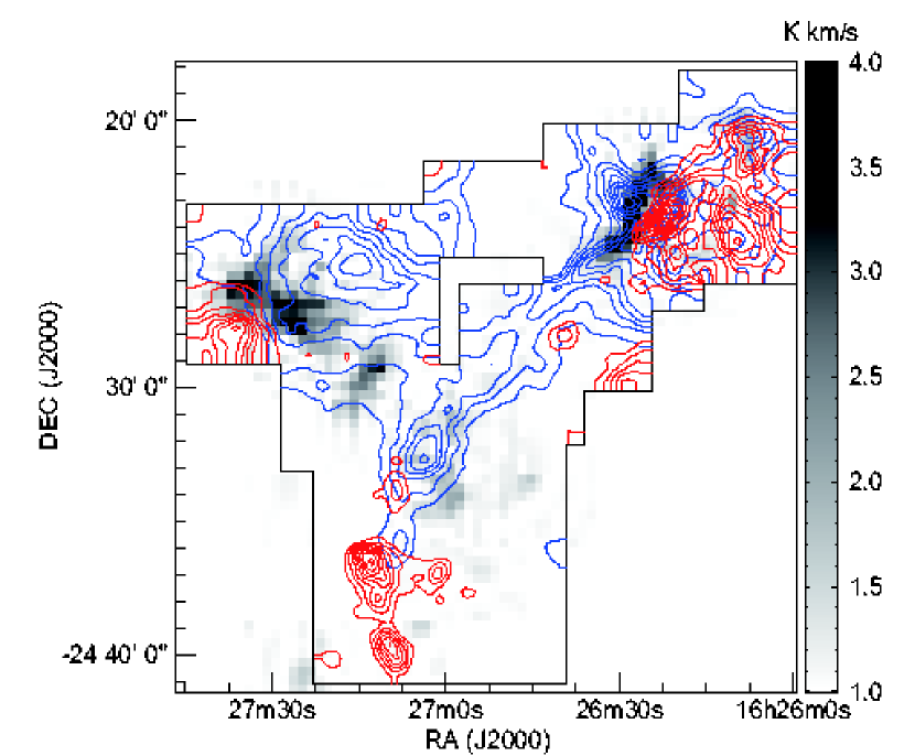
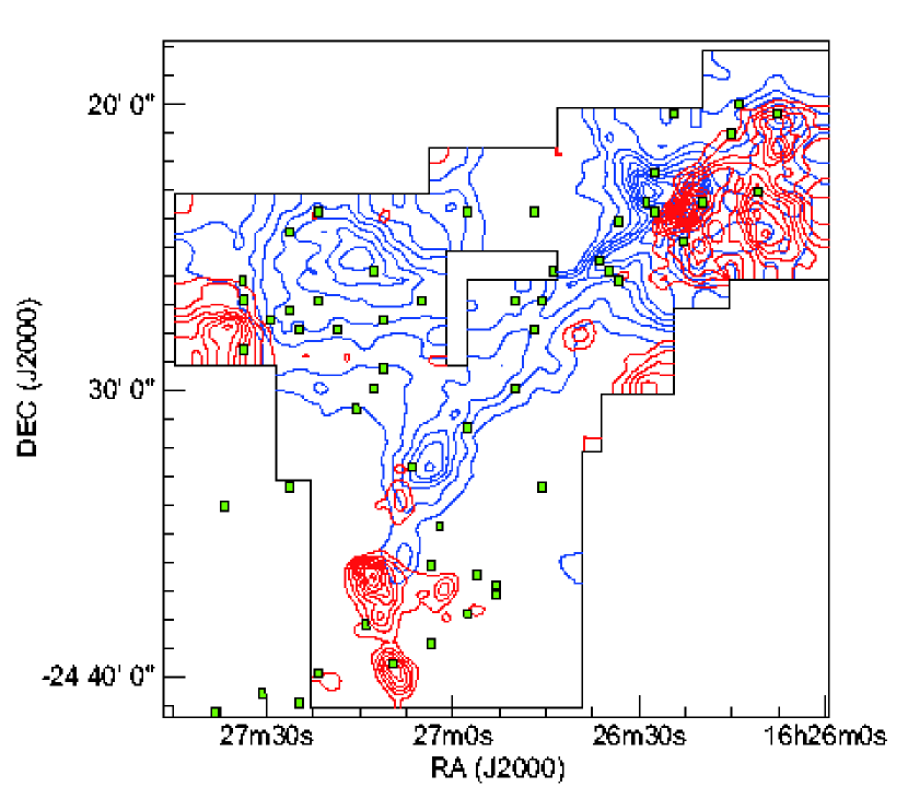
Figure 8: (a) CO ($J=3-2$) map of the $\rho$ Ophiuchi main cloud overlaid on the H¹³CO⁺ ($J=1-0$) integrated intensity map obtained by Maruta et al. (2010) in gray scale. (b) CO ($J=3-2$) map of the $\rho$ Ophiuchi main cloud. The positions of the H¹³CO⁺ cores identified by Maruta et al. (2010) are overlaid by the squares. For both the panels (a) and (b), the blue and red contours are the same as those of Fig. 3.

The blueshifted (north-west) lobe appears to be anti-correlated with the dense gas detected in H¹³CO⁺ emission in the B2 region by Maruta et al. (2010) (see Figure 8a). Around the peak of the CO ($J=3-2$) emission in the blueshifted lobe, the H¹³CO⁺ emission is less prominent, indicating that the dense gas is swept out of the region. In addition, the dense gas well follows the south-east part of the blueshifted lobe, showing an arc-like shape. According to Maruta et al. (2010), a small hole is seen in their H¹³CO⁺ data cube in the southern part of the Oph B2 region (labeled No. 1 in their Figures 2b and 2c), which is located near the north-west edge of the redshifted lobe. Two other holes are also seen near the northern (No. 2 in their Figure 2b, corresponding to the south-east edge of the blueshifted lobe) and southern (No. 3 in their Figure 2b, corresponding to the north-west edge of the redshifted lobe) edges of the B2 region. These holes are likely to be created by the EL 32 outflow. Furthermore, the blueshifted lobe is extended beyond the B2 region, reaching the No. 4 and 5 arcs in Figure 2b of Maruta et al. (2010). These structures suggest that the Oph B2 region is strongly influenced by the EL 32 outflow. See Section 3 of Maruta et al. (2010) for more detail.

Near the southern boundary of the observed area with CO ($J=1-0$) presented in Figure 4, which is outside the CO ($J=3-2$) map, we can see a weak blueshifted and redshifted lobes, which are probably the outflow lobes from IRS 44. This outflow was first discovered by Terebey et al. (1989) by means of the CO ($J=1-0$) interferometric observations using the Owens Valley Millimeter Interferometer. Jørgensen et al. (2009) presented the three-color Spitzer IRAC image of several knots that are proposed to be associated with the outflow from IRS 43 or other nearby YSO including IRS 44 (see their Figure B.1). Although these knots are clearly along a line pointing directly back toward both IRS 43 and 44, the direction of our redshifted lobe of the IRS 44 outflow does not match that suggested by the knots. Thus, these knots are probably not associated with the IRS 44 outflow.

3.3.3 Elias 29 and LFAM 26

In the southern part of the CO ($J=3-2$) map (Figure 3), we can find 4 redshifted (labeled (f), (g), (h), and (i)) and 1 blueshifted (labeled (j)) components. This region was mapped by Bussmann et al. (2007) using the CO ($J=3-2$) emission, but our map covers a larger area than that of Bussmann et al. (2007). The overall feature of the CO ($J=3-2$) map is in good agreement with that of Bussmann et al. (2007), although we found a new redshifted component labeled (i) in the southern part of this region. The redshifted components labeled (h) and (i) and the blueshifted component labeled (j) are most likely to be from a Class I YSO, EL 29. As pointed out by Bussmann et al. (2007), the EL 29 outflow axis has an S-like shape, traced by several H₂ knots detected by Gómez et al. (2003) and Ybarra et al. (2006). In addition, our CO ($J=3-2$) and CO ($J=1-0$) maps in Figures 3 and 4 show that the EL 29 outflow has both the blueshifted and redshifted components on the north side, suggesting that the outflow axis is almost parallel to the plane of the sky. The reason why the EL 29 outflow is so deformed is unclear. One possibility is the interaction with the magnetic field. Recently, the magnetic field structure toward $\rho$ Oph has been mapped by Tamura et al. (2010). They found that the ordered magnetic field penetrates the Oph E and F filaments almost perpendicularly. The direction of the magnetic field coincides well with the outflow axis of the redshifted component. Another possibility is the dynamical interaction with dense gas. In fact, the redshifted outflow lobe is located in the less dense region between the Oph E and F regions. This implies that the outflow hit the dense gas ridge and the direction was altered. Both effects might be responsible for the shape of the redshifted outflow lobe.

On the other hand, we interpret that the other redshifted components (f) and (g) are associated with the outflow from a Class I YSO, LFAM 26, because a line connecting the two H2 knots detected by Khanzadyan et al. (2004), f04-01a and f04-01b, reasonably coincides with a line between the outflow components (f) and (g). Furthermore, the bow-shocked-like shapes of the two knots support our interpretation that the component (g) is coming from LFAM 26. As seen in the CO ($J=1-0$) map in Figure 4, the redshifted components labeled (f) and (g) are also associated with weak blueshifted components, suggesting that the LFAM 26 outflow axis is nearly parallel to the plane of the sky. This interpretation is consistent with the fact that the disk around LFAM 26 is almost edge-on with the rotation axis parallel to the east-west direction (Duchene et al., 2004). Although the VLA 1623 outflow is still the most powerful in this region, the estimated speeds of the EL 29 and LFAM 26 outflows are relatively as large as that of VLA 1623 when the inclination angles of the three outflows are taken into account.

3.4 Derivation of Physical Quantities

In the above subsection, we identified 5 outflows from the CO ($J=3-2$) and CO ($J-1-0$) observations. Here, we derive the physical quantities of the 5 clear outflows, following the procedure described below.

Under the assumption of local thermodynamical equilibrium (LTE) condition and optically thin emission, the molecular outflow masses derived from CO ($J=3-2$) and CO ($J=1-0$) can be calculated, respectively, as

$$M_{\rm 32}=\sum_{j}M_{32,j}\ ,$$ (1)

and

$$M_{\rm 10}=\sum_{j}M_{10,j}\ .$$ (2)

Here, $M_{32,j}$ and $M_{10,j}$ are the outflow masses at the $j$-th channel, derived from CO ($J=3-2$) and CO ($J=1-0$), respectively, and are given by

$$M_{32,j} = 5.0\times 10^{-8}\left({X_{\rm CO}\over 10^{-4}}\right)^{-1}\left({D\over 125{\rm pc}}\right)^{2}\left({\Delta\theta\over{\rm arcsec}}\right)^{2}$$ (3)

$$\times\left({\eta_{32}\over 0.35}\right)^{-1}\left({\sum_{i}T_{A,i,j}^{*}(3-2)\Delta v\over{\rm K\ km\ s^{-1}}}\right)M_{\odot}\ ,$$

and

$$M_{10,j} = 3.4\times 10^{-7}\left({X_{\rm CO}\over 10^{-4}}\right)^{-1}\left({D\over 125{\rm pc}}\right)^{2}\left({\Delta\theta\over{\rm arcsec}}\right)^{2}$$ (4)

$$\times\left({\eta_{10}\over 0.32}\right)^{-1}\left({\sum_{i}T_{A,i,j}^{*}(1-0)\Delta v\over{\rm K\ km\ s^{-1}}}\right)M_{\odot}\ ,$$

where $i$ denotes the grid index on the $j$-th channel. Here, the same excitation temperature $T_{\rm ex}$ of 30 K is adopted for the both lines. The fractional abundance of CO relative to H₂, $X_{\rm CO}$, and the distance to the cloud, $D$, are adopted to be $1\times 10^{-4}$ (a typical value of high-density regions of molecular clouds; e.g., Garden et al. (1991)) and 125 pc (e.g., Lombardi et al., 2008; Loinard et al., 2008; Wilking et al., 2008), respectively. The main beam efficiencies of the ASTE and Nobeyama 45 m telescopes, are $\eta_{\rm 32}=0.35$ and $\eta_{\rm 10}=0.32$, respectively. The integrated intensities of the CO ($J=3-2$) and CO ($J=1-0$) lines at the $i$-th grid are $\eta_{32}^{-1}\sum_{j}T_{A,i,j}^{*}(3-2)\Delta v$ and $\eta_{10}^{-1}\sum_{j}T_{A,i,j}^{*}(1-0)\Delta v$, respectively, where we integrated the antenna temperatures above the 3 $\sigma$ noise levels in the velocity range given in Tables 2 and 3 (see Sections 2.1 and 2.2 for the values of the 1 $\sigma$ rms noise). The symbols $\Delta\theta$ and $\Delta v$ (= 0.4 km s^-1) indicate the grid size and the velocity resolution of the data.

For both the lines, the outflow mass $M_{\rm out}$, the outflow momentum $P_{\rm out}$, and kinetic energy $E_{\rm out}$ are estimated as

$$M_{\rm out}=\sum_{j}M_{j}\ ,$$ (5)

$$P_{\rm out}=\sum_{j}M_{j}|V_{j}-V_{\rm sys}|/\cos\xi\ ,$$ (6)

and

$$E_{\rm out}=\sum_{j}\frac{1}{2}M_{j}(V_{j}-V_{\rm sys})^{2}/\cos^{2}\xi\ ,$$ (7)

respectively, where $M_{j}$ is the mass of the $j$-th channel, $V_{j}$ is the LSR velocity of the $j$-th channel and $V_{\rm sys}$ is the systemic velocity of the driving source. We adopt $V_{\rm sys}\simeq 3.8$, 4.3, 4.9, 4.9, and 4.2 km s^-1 for VLA 1623, EL 32, EL29, LFAM 26, and IRS 44, respectively. Each systemic velocity was determined from the peak $V_{\rm LSR}$ of the H¹³CO⁺ ($J=1-0$) emission averaged in the $2^{\prime}\times 2^{\prime}$ area centered at the position of each source, where we used the H¹³CO⁺ ($J=1-0$) emission of the Nobeyama 45 m archive data whose fits data are available from the Nobeyama web page (http://www.nro.nao.ac.jp/). The systemic velocities are in agreement with the values used by the previous studies: $V_{\rm sys}\simeq 3.7$km s^-1 for VLA 1623 (Kamazaki et al., 2003), 3.9 km s^-1 for EL 32 (Kamazaki et al., 2003), 5 km s^-1 for EL 29 and LFAM 26 (Bussmann et al., 2007), and 3.8 km s^-1 for IRS 44 (Sekimoto et al., 1997). The angle $\xi$ is the inclination angle of an outflow, which is generally uncertain. The three outflows from VLA 1623, EL 29, and LFAM26 in the present paper are expected to be almost parallel to the plane of the sky. Therefore, we adopt $\xi=80^{\circ}$ (see André et al., 1990). For the remaining EL 32 and IRS 44 outflows, we adopt $\xi=57.3^{\circ}$, following Bontemps et al. (1996). The projected maximum size of each outflow lobe, $R_{\rm obs}$, was measured at the 3 $\sigma$ contour in its channel maps. The maximum size of each outflow lobe was estimated by correcting for the projection with the inclination angle $\xi$ as $R_{\rm out}=R_{\rm obs}/\sin\xi$. The velocity range of each outflow was determined using the channel maps: isolated components from high-velocity CO emission are clearly identifiable at more than 3 $\sigma$ level within the velocity range, without significant contamination of emission from the ambient gas. We also note that for all the previously-identified outflows, the velocity ranges for the integration are more or less similar to those listed in Tables 2 and 3.

From these quantities, we calculated the characteristic velocity $V_{\rm out}=P_{\rm out}/M_{\rm out}$, dynamical time $t_{\rm dyn}=R_{\rm out}/V_{\rm out}$, mass loss rate $\dot{M}_{\rm out}=M_{\rm out}/t_{\rm dyn}$, outflow luminosity $L_{\rm out}=E_{\rm out}/t_{\rm dyn}$, and outflow momentum flux $F_{\rm out}=P_{\rm out}/t_{\rm dyn}$. Tables 2 and 3 summarize the outflow parameters derived from the CO ($J=3-2$) and CO ($J=1-0$) data, respectively. The CO lines often become optically thick even toward the outflow wing components. Therefore, the physical parameters such as the outflow mass and momentum listed in Tables 2 and 3, where both the emission lines are assumed to be optically thin, give the lower limits.

Most of the physical quantities estimated from CO ($J=3-2$) and CO ($J=1-0$) are in reasonably good agreement with each other. The total outflow luminosity estimated from CO ($J=3-2$) is only about 6 % larger than that of CO ($J=1-0$). However, for the EL 32 outflow, the mass estimated from CO ($J=1-0$) is larger by a factor of 4 than that of CO ($J=3-2$). This deviation causes large discrepancy in the other quantities such as the momentum, momentum flux, and luminosity. This deviation on the estimated outflow mass is greatest among those of the five outflows. This may imply that the EL 32 outflow is more evolved and thus the outflow gas density may be smaller than the critical density of the CO $(J=3-2)$ transition, $3\times 10^{4}$ cm^-3 . If this is the case, we are probably underestimate the CO ($J=3-2$) outflow mass because of the LTE assumption. This interpretation is consistent with the fact that the dynamical time of the EL 32 outflow is long and that the outflow lobes are most spread out with the widest opening angles.

4 Role of Protostellar Outflows in Clustered Star Formation

4.1 Interaction between the Outflows and Dense Gas in $\rho$ Oph

Recent observations suggest that the dynamical interaction of dense gas with protostellar outflows is likely to trigger the formation of dense cores. For example, Sandell & Knee (2001) performed the 850 $\mu$m dust continuum emission observations toward a nearby pc-scale cluster forming clump, NGC 1333, and found that the dense cores are distributed along multiple shells and filaments that are most likely created by protostellar outflows. Recently, Shimajiri et al. (2008) observed the Orion Molecular Cloud-2 FIR 3/4 regions using the Nobeyama Millimeter Array, and revealed that the ¹²CO emission toward the FIR 4 region shows an L-shaped structure in the position-velocity diagram, suggesting that an outflow from the FIR 3 region compressed the gas in the FIR 4 region, triggering the formation of multiple dense cores in the past few $\times 10^{4}$ yr. These observations suggest that dynamical compression due to protostellar outflows regulates the formation of dense cores in pc-scale cluster forming clumps. Here, we discuss how the outflows in $\rho$ Oph affect the structures of the dense gas.

Using the H¹³CO⁺ ($J=1-0$) data obtained with the Nobeyama 45 m telescope, Maruta et al. (2010) identified 68 dense cores in the central dense region of the $\rho$ Ophiuchi main cloud. The H¹³CO⁺ ($J=1-0$) transition has a critical density of about $10^{5}$ cm^-3, and therefore is suitable as a dense gas tracer. In the following, we compare the H¹³CO⁺ data with the outflows identified in the present paper, to examine whether the outflows are interacting with the dense gas in this region.

The interaction between the CO outflows and the H¹³CO⁺ dense gas seems distinct in the Oph B2 region. In Figure 8a, we present the CO ($J=3-2$) images on the H¹³CO⁺ total integrated intensity map. We also show the positions of the H¹³CO⁺ cores identified by Maruta et al. (2010) in Figure 8b by open squares. About 30 out of 50 H¹³CO⁺ cores located in our CO ($J=3-2$) observed area are distributed around the outflow lobes. For example, in the Oph B2 region, the dense region detected by the H¹³CO⁺ emission has an arc-like shape, following the south-east part of the blueshifted lobe. The part with strong CO ($J=3-2$) emission in the blueshifted lobe appears to be less dense: the peak of the CO ($J=3-2$) blueshifted emission does not correspond to any peak of the H¹³CO⁺ emission.

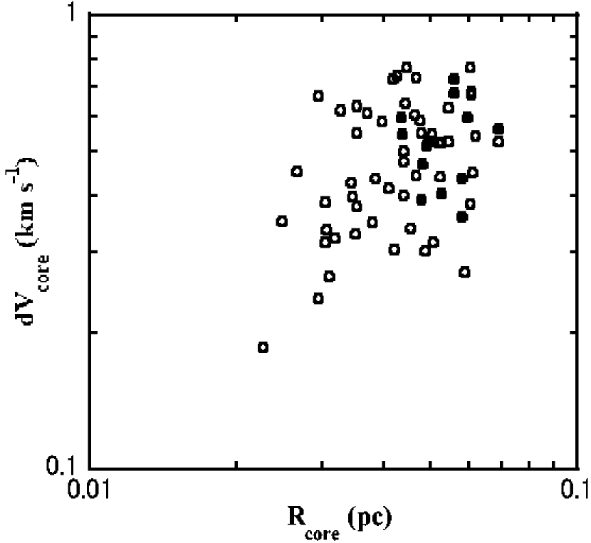
Figure 9: Line-width-radius relation of the H¹³CO⁺ cores identified by Maruta et al. (2010). Filled circles are the cores that appear to be associated with the EL 32 outflow lobes, while open circles the other cores.

The EL 32 outflow possibly injected some energy into the H¹³CO⁺ dense cores. In Figure 9, we present the line-widths of the H¹³CO⁺ cores against their radii, which is essentially the same as Figure 9a of Maruta et al. (2010). The H¹³CO⁺ cores associated with the Oph B2 region, which are indicated by the filled circles, tend to have larger velocity widths. This tendency seems to be consistent with the observations by Friesen et al. (2009), who performed NH₃ observations toward the B1, B2, C, and F regions and found that the NH₃ cores in the B2 region have somewhat larger velocity widths. In addition, they found that the Oph B2 region is slightly warmer ($T\sim 15$ K) than the other regions ($T\sim 12$ K). Friesen et al. (2010) also revealed that the ratio of the NH₃ abundance to N₂H⁺ abundance in the Oph B2 region appears to be smaller than that of the other regions. These facts appear to support the idea that the Oph B2 region is largely affected by the outflow activity. However, there is a possibility that the cores in the B2 region simply tend to follow the line width-radius relation for which the cores with larger radii have larger line widths, although the line-widths of the H¹³CO⁺ cores seem to be almost independent of the core radii for $\rho$ Oph (Maruta et al., 2010). We need further observational evidence to quantify the interaction of the dense gas with the outflow.

In addition to the EL 32 outflow, the VLA 1623 outflow also seems to interact with the dense gas. The head of the collimated blueshifted lobe of the VLA 1623 outflow is located just between the Oph B1 and C regions, which might be broken up into the two parts by the outflow. The No. 33 H¹³CO⁺ core identified by Maruta et al. (2010) appears to collide with the VLA 1623 outflow near the edge of the Oph C region. There are also about 10 H¹³CO⁺ cores that are distributed around the collimated blueshifted lobe of the VLA 1623 outflow.

The redshifted lobe of the EL 29 outflow has an S-shape axis, going through the less dense area between the Oph E and F regions. This suggests that the outflow was presumably bent into an S-shape as a result of the dynamical interaction with the dense filamentary ridge. The redshifted lobe has the two peaks labeled (h) and (i), near which two H¹³CO⁺ cores (No. 34 and 39 in Table 1 of Maruta et al. (2010)) are located. The difference between the radial velocity of the cores ($\simeq 4-5$ km s^-1) and velocity of the redshifted lobe ranges from 2 and 3 km s^-1. Thus, the external pressure exerted on the core surfaces is expected to be significant. In fact, the cores have the virial ratios of 3 $-$ 6, suggesting that they are not gravitationally confined but compressed by the external pressure. Furthermore, the detailed virial analysis performed by Maruta et al. (2010) indicates that most of the cores in $\rho$ Oph seem not to be confined by their self-gravity, but to be confined by the ambient turbulent pressures. This trend is in good agreement with recent numerical simulations of cluster formation by Nakamura & Li (2010, in preparation). These characteristics appear to be consistent with the idea that the outflows trigger the formation of dense cores in the central part of $\rho$ Oph. However, the core distribution projected on the plane of the sky may be just a coincidence. In the 3D space, the cores may not interact with the outflow lobes. To directly verify the interaction with the outflows, we need additional observations such as using SiO and CH₃OH emission, known as shock tracers.

The importance of the external pressures on core dynamical states has been suggested even in the nearby low-mass star forming regions such as the Pipe nebula (Lada et al., 2008). Lada et al. (2008) performed a detailed virial analysis of the cores identified from the extinction map of this region, and found that all the cores have virial ratios larger than unity, suggesting that most of the cores are pressure-confined. However, it is unlikely that the large external pressure is due to the protostellar outflows because star formation activity is quite low in the Pipe nebula (Forbrich et al., 2009). Furthermore, the typical external pressure of the Pipe nebula ($P/k_{B}\sim 8\times 10^{4}$ K cm^-3) is nearly an order of magnitude smaller than that of $\rho$ Oph ($P/k_{B}\sim 3\times 10^{6}$ K cm^-3), where $k_{B}$ is the Boltzmann constant. Lada et al. (2008) proposed that the source of the external pressure is due to the self-gravity of the Pipe nebula itself. In any case, the previous and our studies indicate that the ambient turbulent pressures of the molecular clouds play a significant role in core dynamics for both clustered and distributed star formation.

4.2 A Dynamical Role of the Outflows in $\rho$ Oph

4.2.1 Turbulent Dissipation and Generation

On the basis of numerical simulations, Mac Low (1999) derived the approximated formula for the energy dissipation rate of supersonic turbulence as

$$L_{\rm turb}\simeq f\frac{1/2M\Delta V^{2}}{\lambda_{d}/\Delta V}$$ (8)

where $f(\simeq 0.33)$ is the nondimensional coefficient, $\Delta V$ is the 1D FWHM velocity width, and $\lambda_{d}$ is the driving scale of supersonic turbulence (see equation [7] of Mac Low (1999)). Applying this formula, we evaluate the rate of turbulent energy dissipation in the $\rho$ Ophiuchi main cloud. Loren (1989a) estimated the total gas mass of the whole $\rho$ Ophiuchi main cloud (corresponding to the R21, R22, R24, R25, and R26 regions in his Table 1) to be 883 $M_{\odot}$ using the ¹³CO ($J=1-0$) emission, where the mass is recalculated by using our assumed distance of 125 pc to the cloud. The 1D FWHM velocity width and the mean diameter of $\rho$ Oph (L1688) are estimated to be $\Delta V\simeq 1.5$ km s^-1 and about 1.6 pc, respectively (see Loren, 1989a). The rate of the turbulent energy dissipation is estimated to be

$$L_{\rm turb}\simeq 0.03L_{\odot}\ ,$$ (9)

where we took the cloud diameter as the driving scale of the turbulence. We note that the driving scale of the outflow-driven turbulence is rather uncertain because the driving scale may vary significantly between outflows. In fact, the size of the outflows detected from our observations range from 0.1 pc to 0.6 pc. For example, Maury et al. (2009) adopted the cloud diameter as the driving scale of the outflow-driven turbulence. On the other hand, Arce et al. (2010) adopted the driving scale of 0.2 pc for NGC 1333, although they mentioned that this may be a lower limit because the most outflow lobes they identified in NGC 1333 have larger sizes. From a theoretical consideration, Matzner (2007) derived the driving scale of 0.4 pc for the outflow-driven turbulence. Nakamura & Li (2007) obtained a driving scale similar to that of Matzner (2007) on the basis of the numerical simulations of cluster formation. If we adopt $\lambda_{d}=0.4$ pc, then the energy dissipation rate increases up to $L_{\rm turb}\simeq 0.12L_{\odot}$.

From the analysis in the previous section, we can evaluate the total energy injection rate (mechanical luminosity) due to the protostellar outflows in L1688 as

$$L_{\rm tot}\simeq\sum_{k}{E_{\rm out,{\it k}}\over t_{\rm dyn,{\it k}}}\simeq 0.2L_{\odot}\ .$$ (10)

where $E_{\rm out,{\it k}}$ and $t_{\rm dyn,{\it k}}$ are the outflow energy and dynamical time of the $k$-th outflow, respectively, and we used the quantities obtained from the CO ($J=3-2$) observations. Here, we also included the contribution from small outflows detected in previous observations (Bontemps et al., 1996; Sekimoto et al., 1997; Kamazaki et al., 2003; Stanke et al., 2006). The physical parameters of such outflows are listed in Table 4, where all the quantities have been scaled such that they correspond to an assumed distance of 125 pc. The estimated $L_{\rm tot}$ is sensitive to the inclination angles assumed. If we adopt $\xi=57.3^{\circ}$ (random orientation) for all the outflows, the above value is reduced to $L_{\rm tot}\simeq 0.03L_{\odot}$. The estimated $L_{\rm tot}$ gives a lower limit of the outflow energy injection rate because we assumed the optically thin for the CO line emission and we neglected the contribution from undetected faint outflows. Therefore, we conclude that the total outflow energy injection rate is larger than or at least comparable to the turbulent dissipation rate.

4.2.2 Force Exerted by the Outflows

To clarify how the outflows affect the dynamical state of the cloud, we assess the force balance in the cloud, following Maury et al. (2009). To prevent the global gravitational contraction, the following pressure gradient is needed to achieve the hydrostatic equilibrium:

$${dP_{\rm grav}\over dr}\simeq-G{M(r)\rho(r)\over r^{2}}\left(1-\alpha^{-2}\right)\ ,$$ (11)

where $M(r)$ is the mass contained within the radius $r$ and we assume that the cloud is spherical. The effect of magnetic field is taken into account by the factor $(1-\alpha^{-2})$ and $\alpha$ is the mass-to-magnetic flux ratio normalized to the critical value (e.g., Nakano 1998). Assuming the density profile of $\rho\propto r^{-2}$, the pressure needed to support the cloud against the gravity is estimated to be

$$P_{\rm grav}\simeq{GM(R)^{2}\over 8\pi R^{4}}\left(1-\alpha^{-2}\right)\ .$$ (12)

The force needed to balance the gravitational force is thus evaluated to be

$$F_{\rm grav}\simeq 4\pi R^{2}P_{\rm grav}(R)={GM(R)^{2}\over 2R^{2}}\left(1-\alpha^{-2}\right)\ .$$ (13)

Adopting $M(R)=883M_{\odot}$, $R=0.8$ pc (Loren, 1989a), and $\alpha=1.4$, $F_{\rm grav}$ can be estimated to be

$$F_{\rm grav}=1.3\times 10^{-3}M_{\odot}\ {\rm km\ s^{-1}yr^{-1}}\ ,$$ (14)

where we used the same $\alpha$ as that estimated by Sugitani et al. (2010) for the Serpens main core, a nearby cluster forming clump similar to $\rho$ Oph, although this value is highly uncertain. The moderately strong magnetic field of $\alpha=1.4$ can reduce the gravitational force by a factor of 2. On the other hand, the total force exerted by the outflows in this region is estimated as

$$F_{\rm tot}\simeq\sum_{k}{P_{\rm out,\it k}\over t_{\rm dyn,\it k}}=0.12\times 10^{-3}M_{\odot}\ {\rm km\ s^{-1}\ yr^{-1}}\ .$$ (15)

The force due to the outflows, $F_{\rm tot}$ is one order of magnitude smaller than that needed to stop the global gravitational collapse, $F_{\rm grav}$. Therefore, the force exerted by the outflows seems not to be sufficient for directly supporting the whole cloud against its gravitational collapse. However, we assumed that the emission lines are optically thin in deriving the outflow parameters, and therefore the estimated total force of the outflows gives the lower limit. If we adopt the optical depth of $\tau\sim 5$ for the CO ($J=3-2$) line (Kamazaki et al., 2003), $F_{\rm out}\sim 0.7\times 10^{-3}$ $M_{\odot}$ km s^-1 yr^-1, which is about a half of $F_{\rm grav}$. If this is the case, the force exerted by the outflows may significantly contribute to the cloud support. The accurate estimate of the optical depth is necessary to clarify the dynamical role of the outflows on the cloud support.

4.2.3 Comparison with other nearby cluster forming clumps

Recent observations of nearby cluster forming regions have revealed the detailed structure of pc-scale dense clumps and star formation activity including the outflows. Here, using the same method as in Section 4.2.2, we compare the dynamical states of two nearby cluster forming clumps, NGC 1333 and Serpens, with $\rho$ Oph.

Table 5 shows the global properties of the nearby cluster forming clumps. For the Serpens clump, we adopted the results of Sugitani et al. (2010) who used the outflow parameters estimated by Davis et al. (1999). For NGC 1333, we estimated the physical quantities using the outflow parameters obtained by Sandell & Knee (2001) and the clump mass obtained by Ridge et al. (2003). The outflow parameters listed in Table 5 are estimated under the assumption of optically thin. Therefore, they give the lower limits. Recently, for NGC 1333, Arce et al. (2010) performed a detailed analysis on the effect of outflows in the parent clump using the ¹²CO ($J=1-0$) and ¹³CO ($J=1-0$) lines, taking into account the effect of opacity. The virial mass is estimated from the total mass and mean FWHM velocity width as

$$M_{\rm VIR}=210a^{-1}\left(\frac{R_{\rm cl}}{\rm pc}\right)\left(\frac{\Delta V}{\rm km\ s^{-1}}\right)^{2}M_{\odot}$$ (16)

where the dimensionless parameter $a$ is set to $5/3$, corresponding to the density profile of $\rho\propto r^{-2}$. The cloud masses, velocity widths, and cloud radii are adopted from the references indicated in the caption of Table 5. For all the clumps, the energy injection rate of the outflows seems larger than or comparable to the turbulent dissipation rate. Thus, we expect that the protostellar outflows can power supersonic turbulence in these three pc-scale cluster forming clumps. Our analysis also indicates that for Serpens and NGC 1333, the outflows can exert the significant force against global gravitational collapse. However, for $\rho$ Oph, the total force of the observed outflows appears not to be enough to support the whole cloud even if we correct the effect of opacity by a factor of $\sim 5$. In fact, the virial ratio is quite small, and the clump should collapse globally. We note that the estimated virial ratio of $\rho$ Oph is insensitive to the adopted line. For example, if we use the C¹⁸O ($J=1-0$) emission, the virial ratio is estimated to be about 0.2, where we adopted the cloud mass of 494 $M_{\odot}$, the velocity width of about 1.6 km s^-1, and the radius of about 0.3 pc from Tachihara et al. (2000).

Why is the estimated virial ratio of $\rho$ Oph so small? One possibility is that the current star formation got less active than before, and therefore the cloud turbulence dissipated significantly. According to Evans et al. (2009), the current star formation rate appears to be smaller than the value averaged over the cloud lifetime for $\rho$ Oph. In fact, Loren (1989b) obtained a very shallow linewidth-radius relation for the $\rho$ Oph clump, based on the ¹³CO ($J=1-0$) observations. The shallow linewidth-radius relation might suggest that the large-scale turbulent motions have dissipated significantly because of the lack of the large-scale energy injection events. If this is the case, the clump as a whole might be in the course of the large-scale gravitational collapse. Another possibility is that the $\rho$ Oph clump as a whole has been compressed by a large-scale shock, which has enhanced the cloud gravitational energy, reducing the virial ratio of the clump significantly. Several previous studies suggest that the $\rho$ Oph cloud has been compressed by an expanding shell created by stellar winds and supernova explosions in the Sco OB2 association, and star formation in this cloud has been externally triggered (Vrba, 1977; Meyers et al., 1985; Loren & Wootten, 1986; de Geus, 1992; Motte et al., 1998; Tachihara et al., 2002). The cloud morphology and kinematics appear to support this scenario. For example, the south-western side of the cloud has a sharp edge, whereas the north-eastern side has a less dense elongated structure. This is consistent with the scenario that the shell passing through the cloud from the south-western side to the north-eastern side would compress the cloud. The expanding shell is also observed with the HI emission. In addition, Motte et al. (1998) revealed that the dense cores as well as several YSOs appear to be distributed along a linear chain that is roughly perpendicular to the direction of shock propagation. They proposed that the large-scale shock has compressed the cloud to create a dense ridge that has fragmented into many cores to form stars. Meyers et al. (1985) suggested that the velocity difference of $\lesssim$ 10 km s^-1 between optical absorption lines of CH and CH⁺ is caused by the shock transmitted into the dense clump. This yields the cloud-crushing time of $t_{cc}\sim{\rm a\ few}\ 10^{5}$ yr, which is about 5 $-$ 10 times shorter than the typical age of the YSOs in this clump. Here, the cloud crushing time $t_{cc}$ is the timescale for the cloud to be crushed by the shock transmitted into the cloud. According to numerical simulations of the interaction of a large-scale shock with a cloud, the shock motions are converted into the cloud turbulence sufficiently within several cloud crushing times (see e.g., Nakamura et al., 2006). The large-scale shocks are sometimes considered to be one of the important driving sources of the cloud turbulence (e.g., McKee & Ostriker, 2007). For $\rho$ Oph, the observed turbulent motions seem too weak to support the whole cloud against the global gravitational collapse, although the shock due to the large-scale expanding shell has passed over some $\sim$10 $t_{cc}$ ago. The large-scale shock seems not to have been sufficient to supply the supersonic cloud turbulence in this clump.

Using the ¹³CO ($J=1-0$) data, Padoan et al. (2009) derived the power spectrum of the turbulent field in NGC 1333 and claimed that there is no evidence of outflow-driven turbulence in NGC 1333. This result apparently contradicts our conclusion. However, the ¹³CO emission can trace only tenuous inter-core gas with densities as low as $10^{3}$ cm^-3. Thus, their power spectrum is likely to be contaminated by the ambient components that are not associated with the dense cluster forming clump whose typical density is $10^{4}$ cm^-3. In addition, it is difficult to detect protostellar outflows from the ¹³CO ($J=1-0$) line because of its weak emission at the high-velocity wings. The line also tends to be strongly optically thick toward cluster forming clumps. Therefore, the ¹³CO emission may not be suitable for searching the influence by protostellar outflows in molecular clouds. More careful analysis will be needed. Denser molecular gas tracers such as the C¹⁸O ($J=1-0$) line are likely to be more appropriate for this kind of analysis. In fact, Brunt et al. (2009) investigated the turbulent field in NGC 1333 on the basis of the PCA analysis using the ¹²CO, ¹³CO, and C¹⁸O emission, and found that the power index of the turbulent spectrum derived from C¹⁸O is significantly shallower than those of ¹²CO and ¹³CO , implying that the outflows are likely to be responsible for the turbulence generation in the pc-scale cluster forming clump (see also Arce et al., 2010). This result supports our conclusion.

5 Summary

We summarize the primary results of the present paper as follows.

1. We have performed the CO ($J=3-2$) and CO ($J=1-0$) observations toward the nearest pc-scale cluster forming clump, $\rho$ Ophiuchi main cloud, and identified 5 outflows, whose driving sources are VLA 1623, EL 32, LFAM26, EL29, and IRS 44. We found that the EL 32 and EL 29 outflows identified by the previous studies are larger than previously mapped.

2. We estimated the physical quantities of the outflows. The most luminous outflow was found to be the one from VLA 1623. We also discovered that the EL 32 outflow has the largest mass and momentum among the identified outflows. The physical quantities estimated from the two lines reasonably agree with each other.

3. We compared our outflow images with the H¹³CO⁺ map obtained by Maruta et al. (2010), and found that 30 out of 50 H¹³CO⁺ cores appear to overlap with the outflow lobes on the plane of the sky. This might imply that the outflows influence the dense cores significantly.

4. We estimated the physical parameters of the identified outflows and measured the total outflow energy injection rate and momentum flux. The total outflow energy injection rate is significantly larger than the dissipation rate of the supersonic turbulence in this region. We conclude that the outflows can power the supersonic turbulence in this region.

In contrast, the outflows do not have enough momentum flux to support the whole clump against the global gravitational contraction. However, this result is sensitive to the assumed optical depth for the CO lines. If the CO lines are optically thick, then the contribution of the outflow force to the cloud support is expected to be significant. The accurate estimate of the optical depth for the CO lines toward the outflows is needed for further clarification of the role of the outflows on the cloud support.

5. Using the literatures, we applied the same analysis to the two nearby pc-scale cluster forming clumps: Serpens and NGC 1333, and obtained the total energy injection rates and momentum fluxes. Our analysis indicates that for both the cluster forming clumps, the outflows are likely to play a significant role in the global cloud support and turbulence generation.

6. The virial ratio of $\rho$ Oph is estimated to be only 0.2 even if the contribution of the moderately strong magnetic support against global collapse is taken into account. Such a small virial ratio might suggest that the current star formation is inactive, and thus energy injection from the forming stars is not sufficient to support the clump. Alternatively, the small virial ratio might be a result of the large-scale shock compression. The observed weak cloud turbulence may suggest that the large-scale shock due to supernovae cannot supply the supersonic turbulence significantly to this cloud. Instead, the large-scale shock may have triggered further star formation by increasing the gravitational energy.

Appendix A Mass of Molecular Outflows

In this Appendix, we derive an expression for the outflow mass calculated from the CO ($J=3-2$) and CO ($J=1-0$) emission under the assumption of local thermodynamic equilibrium (LTE) with the populations of all levels characterized by a single excitation temperature, $T_{\rm ex}$. The CO ($J=3-2$) and CO ($J=1-0$) emission associated with the molecular outflows is also assumed to be optically thin. In this sense, our estimated outflow masses are the lower limit.

For molecular gas in LTE, the optical depth for the transition from upper level, $J+1$, to lower level, J, is given by

$$\tau_{\nu}={c^{2}A_{J+1,J}\over 8\pi\nu^{2}}{2J+3\over 2J+1}\left[1-\exp\left(-{h\nu\over k_{B}T_{\rm ex}}\right)\right]{n_{J}L\over d\nu}\ ,$$ (A1)

where $c$ is the speed of light, $A_{J+1,J}$ is Einstein’s A coefficient for the transition from the upper level to the lower level, $\nu$ is the frequency of the transition, $k_{B}$ is the Boltzmann constant, $n_{J}$ is the density of the molecule in the lower level, $J$, and $L$ is the thickness along the line of sight [$A_{10}=7.203\times 10^{-8}$ s^-1 and $A_{32}=2.497\times 10^{-6}$ s^-1 for CO ($J=1-0$) and CO ($J=3-2$), respectively.].

The column density of the molecule in the lower level $J$ is then estimated as

$$N_{J}=\int n_{J}Ld\nu=\frac{8\pi\nu^{3}}{c^{3}A_{J+1,J}}{2J+1\over 2J+3}\left[1-\exp\left(-{h\nu\over k_{B}T_{\rm ex}}\right)\right]^{-1}\int\tau_{v}dv\ ,$$ (A2)

where the relation $d\nu=(\nu/c)dv$ is used.

The column density of the molecule in the lower level $J$ is also expressed using the total column density, $N_{\rm tot}$, as

$$N_{J}={2J+1\over Z(T_{\rm ex})}N_{\rm tot}\exp\left[-\frac{hBJ(J+1)}{k_{B}T_{\rm ex}}\right]\ ,$$ (A3)

and

$$Z(T_{\rm ex}) = \sum_{J=0}^{\infty}(2J+1)\exp\left[-\frac{hBJ(J+1)}{k_{B}T_{\rm ex}}\right]$$ (A4)

$$\approx {k_{B}T_{\rm ex}\over hB}\left[1+{1\over 3}{hB\over k_{B}T_{\rm ex}}+{1\over 15}\left({hB\over k_{B}T_{\rm ex}}\right)^{2}\right]\ ,$$ (A5)

where $Z$ is the partition function and $B$ is the rotational constant ($B=57.8975$ GHz for CO). From eq. [A2], we thus obtain the expression for the total column density as

$$N_{\rm tot}={8\pi\nu^{3}\over c^{3}A_{J+1,J}(2J+3)}Z(T_{\rm ex})\exp\left[-\frac{hBJ(J+1)}{k_{B}T_{\rm ex}}\right]\left[1-\exp\left(-{h\nu\over k_{B}T_{\rm ex}}\right)\right]^{-1}\int\tau_{v}dv\ .$$ (A6)

The optical depth $\tau_{\nu}$ can be obtained from the expression for the antenna temperature at the frequency $\nu$:

$$T_{A}^{*}=\eta{h\nu\over k_{B}}\left[f(T_{\rm ex})-f(T_{\rm bg})\right]\left[1-\exp\left(-\tau_{\nu}\right)\right]\approx\eta{h\nu\over k_{B}}\left[f(T_{\rm ex})-f(T_{\rm bg})\right]\tau_{\nu}\ ,$$ (A7)

and

$$f(T)\equiv{1\over\exp(h\nu/k_{B}T)-1}\ ,$$ (A8)

where $\eta$ is the beam efficiency and $T_{\rm bg}$ is the temperature of the background radiation. The beam dilution factor is set to unity. We adopt the cosmic microwave background radiation with $T_{\rm bg}=2.7$ K as the background radiation. Then, the value of $f(T_{\rm ex})$ is much larger than $f(T_{\rm bg})$ when $T_{\rm ex}\sim 30$ K, the adopted value in the present paper.

Therefore, we neglect the second term in the right hand side of eq. [A7], $f(T_{\rm bg})$. The column density at the $i$-th grid on the $j$-th channel is then given using the relation $\nu=2B(J+1)$ by

$$N_{\rm tot,{\it i,j}}={8\pi k_{B}\nu^{2}\over hc^{3}A_{J+1,J}(2J+3)}Z(T_{\rm ex})\exp\left[\frac{hB(J+1)(J+2)}{2k_{B}T_{\rm ex}}\right]\eta^{-1}T_{A,i,j}^{*}\Delta v\ .$$ (A9)

Thus, the outflow mass calculated from the CO ($J=3-2$) and CO ($J=1-0$) emission is given, respectively, by

$$M_{32}=\sum_{j}M_{32,j}\ ,$$ (A10)

and

$$M_{10}=\sum_{j}M_{10,j}\ ,$$ (A11)

where

$$M_{32,j} = \mu m_{\rm H}X_{\rm CO}^{-1}\Omega D^{2}\sum_{i}N_{\rm tot,\it i,j}$$ (A12)

$$= 9.4\times 10^{-10}\left({X_{\rm CO}\over 10^{-4}}\right)^{-1}\left({D\over 125{\rm pc}}\right)^{2}\left({\Delta\theta\over{\rm arcsec}}\right)^{2}\left({\eta_{32}\over 0.35}\right)^{-1}\left({\sum_{i}T_{A,i,j}^{*}\Delta v\over{\rm K\ km\ s^{-1}}}\right)$$

$$\times T_{\rm ex}\exp\left[{16.6\ {\rm K}\over T_{\rm ex}}\right]\left[1+{1\over 3}\left({T_{\rm bg}\over T_{\rm ex}}\right)+{1\over 15}\left({T_{\rm bg}\over T_{\rm ex}}\right)^{2}\right]M_{\odot}\ ,$$

and

$$M_{10,j} = 9.2\times 10^{-9}\left({X_{\rm CO}\over 10^{-4}}\right)^{-1}\left({D\over 125{\rm pc}}\right)^{2}\left({\Delta\theta\over{\rm arcsec}}\right)^{2}\left({\eta_{10}\over 0.32}\right)^{-1}\left({\sum_{i}T_{A,i,j}^{*}\Delta v\over{\rm K\ km\ s^{-1}}}\right)$$ (A13)

$$\times T_{\rm ex}\exp\left[{5.53\ {\rm K}\over T_{\rm ex}}\right]\left[1+{1\over 3}\left({T_{\rm bg}\over T_{\rm ex}}\right)+{1\over 15}\left({T_{\rm bg}\over T_{\rm ex}}\right)^{2}\right]M_{\odot}\ .$$

Here, $i$ is the grid index on the $j$-th channel, $\eta_{32}$ and $\eta_{10}$ are the main beam efficiencies of the ASTE and Nobeyama 45 m telescopes, respectively, $m_{\rm H_{2}}$ is the mass of a hydrogen molecule, $X_{\rm CO}$ is the fractional abundance of CO relative to H₂, and $\mu$ is the mean molecular weight of the gas and is set to 2.33. $\Omega$ is the solid angle of the object and $D$ is the distance to the object.

Table 1: Molecular Outflows Identified in the Present Paper

Name	Region	Reference	Characteristics
VLA 1623	Oph A	1,2,3,6,7	Class 0, highly-collimated, strong blueshifted lobe
EL32	Oph B2	1,7	Class I, very extended lobes, most massive and most luminous
EL29	Oph E	1,3,4,5,8	Class I
LFAM 26	Oph E	1,4	Class I
IRS 44	Oph F	1,4,8	Class I

Table 2: Molecular Outflow Parameters Obtained From CO ($J=3-2$)

Name	Velocity Range	$V_{\rm out}$	$R_{\rm out}$	$M_{\rm out}$	$P_{\rm out}$	$t_{\rm dyn}$	$\dot{M}_{\rm out}$	$F_{\rm out}$	$L_{\rm out}$	Position
	(km s-1)	(km s-1)	(pc)	($10^{-2}M_{\odot}$)	($M_{\odot}$km s-1)	($10^{4}$ yr)	($M_{\odot}$yr-1)	($M_{\odot}$km s-1yr-1)	($10^{-2}L_{\odot}$)
Blue Lobe
VLA 1623	$-5.0\sim 1.0$	21.7	0.51	2.2	0.49	2.3	$9.8\times 10^{-7}$	$2.1\times 10^{-5}$	4.2	S-E
VLA 1623	$-5.0\sim 1.0$	20.4	0.098	0.55	0.11	0.47	$1.2\times 10^{-7}$	$2.4\times 10^{-5}$	4.3	N-W
EL 32	$-5.0\sim 0.5$	9.73	0.25	2.3	0.22	2.6	$8.8\times 10^{-7}$	$8.6\times 10^{-6}$	0.71	N-W
LFAM 26	$-5.0\sim 1.0$	29.9	0.089	0.022	0.0065	0.29	$7.5\times 10^{-8}$	$2.2\times 10^{-6}$	0.73	W
EL 29	$-5.0\sim 1.0$	21.6	0.083	0.11	0.025	0.38	$3.0\times 10^{-7}$	$6.5\times 10^{-6}$	1.3	N
Red Lobe
VLA 1623	$6.5\sim 13.0$	22.7	0.096	0.25	0.056	0.41	$6.0\times 10^{-7}$	$1.4\times 10^{-5}$	2.9	N-E
EL 32	$6.5\sim 10.0$	5.7	0.17	0.50	0.028	2.9	$1.7\times 10^{-7}$	$9.7\times 10^{-7}$	0.049	S-E
LFAM 26	$6.5\sim 12.0$	19.4	0.11	0.25	0.048	0.55	$4.5\times 10^{-7}$	$8.6\times 10^{-6}$	1.5	E
LFAM 26	$7.0\sim 12.0$	24.2	0.0089	0.037	0.089	0.36	$1.0\times 10^{-7}$	$2.5\times 10^{-6}$	0.55	W
EL 29	$6.5\sim 12.0$	21.6	0.13	0.22	0.047	0.60	$3.7\times 10^{-7}$	$8.0\times 10^{-6}$	1.5	S

Note. — The CO ($J=3-2$) emission lines are assumed to be optically thin. Therefore, the physical quantities listed here give the lower limits.

Table 3: Molecular Outflow Parameters Obtained From CO ($J=1-0$)

Name	Velocity Range	$V_{\rm out}$	$R_{\rm out}$	$M_{\rm out}$	$P_{\rm out}$	$t_{\rm dyn}$	$\dot{M}_{\rm out}$	$F_{\rm out}$	$L_{\rm out}$	Position
	(km s-1)	(km s-1)	(pc)	($10^{-2}M_{\odot}$)	($M_{\odot}$km s-1)	($10^{4}$yr)	($M_{\odot}$yr-1)	($M_{\odot}$km s-1yr-1)	($10^{-2}L_{\odot}$)
Blue Lobe
VLA 1623	$-3.0\sim 1.0$	20.8	0.52	3.9	0.78	2.5	$1.5\times 10^{-6}$	$3.2\times 10^{-5}$	5.8	S-E
VLA 1623	$-3.0\sim 1.0$	18.8	0.084	0.34	0.065	0.44	$8.0\times 10^{-7}$	$1.5\times 10^{-5}$	2.3	N-W
EL 32	$-3.0\sim 0.5$	9.4	0.22	10.0	0.94	2.3	$4.4\times 10^{-6}$	$4.1\times 10^{-5}$	3.3	N-W
LFAM 26	$-3.0\sim 1.5$	20.7	0.053	0.023	0.0050	0.25	$9.5\times 10^{-8}$	$1.9\times 10^{-6}$	0.33	E
EL 29	$-3.0\sim 1.5$	13.5	0.074	0.25	0.033	0.54	$4.7\times 10^{-7}$	$6.2\times 10^{-6}$	0.69	N
IRS 44	$-3.0\sim 1.0$	8.7	0.036	0.15	0.013	0.40	$3.7\times 10^{-7}$	$3.2\times 10^{-6}$	0.26	S-W
Red Lobe
EL 32	$6.5\sim 9.0$	4.6	0.31	3.2	0.15	6.5	$5.0\times 10^{-7}$	$2.3\times 10^{-6}$	0.087	S-E
LFAM 26	$6.5\sim 9.0$	15.8	0.10	0.31	0.048	0.64	$4.8\times 10^{-7}$	$7.6\times 10^{-6}$	0.99	E
LFAM 26	$6.5\sim 9.0$	15.4	0.068	0.045	0.0070	0.43	$1.0\times 10^{-7}$	$1.7\times 10^{-6}$	0.21	W
EL 29	$6.5\sim 9.0$	17.6	0.096	0.34	0.062	0.54	$6.5\times 10^{-7}$	$9.7\times 10^{-6}$	1.7	S
EL 29	$6.5\sim 9.0$	16.9	0.083	0.21	0.034	0.48	$4.3\times 10^{-7}$	$7.2\times 10^{-6}$	1.0	N
IRS 44	$6.5\sim 9.0$	8.4	0.089	0.14	0.012	1.0	$1.3\times 10^{-7}$	$1.1\times 10^{-6}$	0.083	N

Note. — The CO ($J=1-0$) emission lines are assumed to be optically thin. Therefore, the physical quantities listed here give the lower limits.

Table 4: Molecular Outflow Parameters Compiled From the Literature in the $\rho$ Ophiuchi Main Cloud

Name	$V_{\rm out}$	$M_{\rm out}$	$F_{\rm out}$	$L_{\rm out}$	Reference
	(km s-1)	($M_{\odot}$)	($M_{\odot}$ km s-1 yr-1)	($L_{\odot}$)
WL 6	7.5	$1.5\times 10^{-3}$	$2.0\times 10^{-6}$	$1.2\times 10^{-3}$	1
WL 10	7.5	$5.7\times 10^{-3}$	$3.5\times 10^{-6}$	$2.2\times 10^{-3}$	1
AN	3	$8.2\times 10^{-3}$	$2.6\times 10^{-6}$	$7.0\times 10^{-3}$	2
AS	2	$2.9\times 10^{-3}$	$3.7\times 10^{-6}$	$2.9\times 10^{-3}$	2
MMS126	6.5	$1.0\times 10^{-3}$	$0.19\times 10^{-6}$	$0.059\times 10^{-3}$	3
WL 12			$1.4\times 10^{-6}$		4
IRS 43			$3.4\times 10^{-6}$		4
IRS 48			$6.9\times 10^{-6}$		4
IRS 51			$1.3\times 10^{-6}$		4

Note. — All the quantities listed in the table are corrected to $D=125$ pc under the assumption that observed lines are optically thin. The values of outflow mechanical luminosities for WL 5, and WL 10 are estimated from the expression $L_{\rm out}=F_{\rm out}V_{\rm out}/2$.

Table 5: Global Properties of Nearby Cluster Forming Clumps

Name	Distance	Mass	Radius	Velocity Width	Virial Ratio	$L_{\rm turb}$	$L_{\rm tot}$	$F_{\rm grav}$	$F_{\rm tot}$
	(pc)	($M_{\odot}$)	(pc)	(km s-1)		($L_{\odot}$)		($M_{\odot}$ km s-1 yr-1)
Serpens 1	260	210	0.46	2.0	1.1	0.14 $-$ 0.32	1.3	$1.9\times 10^{-4}$	5.2$\times 10^{-4}$
$\rho$ Oph 2	125	883	0.8	1.5	0.22	0.06 $-$ 0.12	0.2	$1.3\times 10^{-3}$	$1.2\times 10^{-4}$
NGC 1333 3	220	573	0.44	2.8	0.76	0.41 $-$ 0.90	0.65	$1.8\times 10^{-3}$	$6.0\times 10^{-4}$

Note. — Reference: ¹Sugitani et al. (2010), ²this paper, ³Knee & Sandell (2000). For all the clumps, the contribution of magnetic support is taken into account for estimation of $F_{\rm grav}$ whose value is reduced by a factor of about 2. See Sugitani et al. (2010) in detail. The outflow parameters listed in the table are the lower limits because they are estimated under the assumption that the lines are optically thin.

References

- Allen et al. (2006) Allen, L. et al. 2006. in Protostars and Planets V, eds. B. Reipurth, D. Jewitt, and K. Keil (The University of Arizona Press), p. 361
- André et al. (1990) André, P., Martin-Pintado, J., Despois, D., & Montmerle, T. 1990, A&A, 236, 180
- Arce et al. (2010) Arce, H. G., Borkin, M. A., Goodman, A. A., Pineda, J. E., & Halle, M. W. 2010, ApJin press
- Bally et al. (1996) Bally, J., Devine, D., & Reipurth, B. 1996, ApJ, 473, 49
- Bontemps et al. (1996) Bontemps, S., André, P., Terebey, S., & Cabrit, S. 1996, A&A, 311, 858
- Brunt et al. (2009) Brunt, C. M., Heyer, M. H., & Mac Low, M.-M. 2009, ApJ, 504, 883
- Bussmann et al. (2007) Bussmann, R. S., Wong, T. W., Hedden, A. S., Kulesa, C. A., & Walker, C. K. ApJ, 657, L33
- Carpenter (2000) Carpenter, J. M. 2000, ApJ, 120, 139
- Carroll et al. (2009) Carroll, J. J., Frank, A., Blackman, E. G., & Cunningham, A. J., & Quillen, A. C. 2009, ApJ, 695, 1376
- Carroll et al. (2010) Carroll, J. J., Frank, A., & Blackman, E. G. 2010, submitted to ApJ (arXiv:1005.1098)
- Ceccarelli et al. (2002) Ceccarelli, C., Boogert, A. C. A., Tielens, A. G. G. M., Caux, E., Hogerheijde, M. R., & Parise, B. 2002, A&A, 395, 863
- Cunningham et al. (2006) Cunningham, A., Frank, A., Quillen, A., & Blackman, E. 2006, ApJ, 653, 416
- Davis et al. (1999) Davis, C. J., Matthews, H. E., Ray, T. P., Dent, W. R. F., & Richer, J. S. 1999, MNRAS, 309, 141
- Duchene et al. (2004) Duchene, G., Bouvier, J., Bontemps, S., Andre , P., & Motte, F. 2004, A&A, 427, 651
- de Geus (1992) de Geus, E.J. 1992, A&A, 262, 258
- Dent et al. (1995) Dent, W. R. F., Matthews, H. E., & Walther, D. M. 1995, MNRAS, 277, 193
- Ezawa et al. (2004) Ezawa, H., Kawabe, R., Kohno, K., & Yamamoto, S. 2004, Proc. SPIE, 5489, 763
- Evans et al. (2009) Evans, N. J. et al. 2009, ApJS, 181, 321
- Forbrich et al. (2009) Forbrich, J., Lada, C. J., Muench, A. A., Alves, J., & Lombardi, M. 2009, ApJ, 704, 292
- Friesen et al. (2009) Friesen, R. K., Di Francesco, J., Shirley, Y. L., & Myers, P. C., 2009, ApJ, 697, 1457
- Friesen et al. (2010) Friesen, R. K., Di Francesco, J., Shimajiri, Y., & Takakuwa, S., 2010, ApJ, 708, 1002
- Garden et al. (1991) Garden, R. P., Hayashi, M., Gatley, I., Hasegawa, T., & Kaifu, N. 1991, ApJ, 374, 540
- Gómez et al. (2003) Gómez, M., Stark, D. P., Whitney, B. A.,& Churchwell, E. 2003, AJ, 126, 863
- Gutermuth et al. (2009) Gutermuth, R. A., Myers, P. C., Megeath, S. T., Allen, L. E., Pipher, J. L., Muzerolle, J., Porras, A., Winston, E., & Fazio, G. 2009, ApJ, 674, 336
- Hatchell et al. (2007) Hatchell, J., Fuller, G. A., & Richer, J. S. 2007, A&A, 472, 187
- Hatchell & Dunham (2009) Hatchell, J. & Dunham, M. M. 2009, A&A, 502, 139
- Higuchi et al. (2009) Higuchi, A., Kurono, Y., Saito, M., & Kawabe, R. 2009, ApJ, 705, 468
- Hiramatsu et al. (2010) Hiramatsu, M., Hirano, N., Takakuwa, S. 2010, ApJ, 712, 778
- Johnstone et al. (2000) Johnstone, D., Wilson, C. D., Moriarty-Schieven, G., Joncas, G., Smith, G., Gregersen, E., & Fich, M. 2000, ApJ, 545, 327
- Jørgensen et al. (2008) Jørgensen, J. K., Johnstone, D., Kirk, H., Myers, P. C., Allen, L. E., & Shirley, Y. L. 2008, ApJ, 683, 822
- Jørgensen et al. (2009) Jørgensen, J. K., van Dishoeck, E. F., Visser, R., Bourke, T. L., Wilner, D. J., Lommen, D., Hogerheijde, M. R., & Myers, P. C. 2009, A&A, 507, 861
- Kamazaki et al. (2003) Kamazaki, T., Saito, M., Hirano, N., Umemoto, T. & Kawabe, R. ApJ, 2003, 584, 357
- Khanzadyan et al. (2004) Khanzadyan, T., Gredel, R., Smith, M. D., & Stanke, T. 2004, A&A, 426, 171
- Knee & Sandell (2000) Knee, L. B. G. & Sandell, G. 2000, A&A, 361, 671
- Lada et al. (1991) Lada, E. A., Bally, J., & Stark, A. A. 1991, ApJ, 368, 432
- Lada et al. (2008) Lada, C. J., Muench, A. A., Rathborne, J., Alves, J. F., & Lombardi, M. 2008, ApJ, 672, 410
- Lada & Lada (2003) Lada, C. J. & Lada, E. A. ARA&A, 2003, 41, 57
- Li & Nakamura (2006) Li, Z.-Y. & Nakamura, F. ApJ, 2006, 640, L187
- Li et al. (2010) Li, Z.-Y., Wang, P., Abel, T., & Nakamura, F. ApJ, 2010, 720, L26
- Loinard et al. (2008) Loinard, L., Torres, R. M., Mioduszewski, A. J. & Rodriguez, L. F. 2008, ApJ, 675, L29
- Lombardi et al. (2008) Lombardi, M., Lada, C. J. & Alves, J. 2008, A&A, 480, 785
- Loren & Wootten (1986) Loren, R.B., & Wootten, A. 1986, ApJ, 306, 142
- Loren (1989a) Loren, R. B. 1989a, ApJ, 338, 902
- Loren (1989b) Loren, R. B. 1989b, ApJ, 338, 925
- Mac Low (1999) Mac Low, M.-M. 1999, ApJ, 524, 169
- Matzner & McKee (2000) Matzner, C. D. & McKee, C. F. ApJ, 2000, 545, 364
- Matzner (2007) Matzner, C. D. ApJ, 2007, 659, 1394
- Maruta et al. (2010) Maruta, H., Nakamura, F., Nishi, R., Ikeda, N., & Kitamura, Y. 2010, ApJ, 714, 680
- Maury et al. (2009) Maury, A. J. André, P., & Li, Z.-Y. 2009, A&A, 499, 175 submitted to ApJ
- Meyers et al. (1985) Meyers, K.A., Snow, T.P., Federman, S.R., & Breger, M. 1985, ApJ, 288, 148
- McKee (1989) McKee, C. F. 1989, ApJ, 345, 782
- McKee & Ostriker (2007) McKee, C. F., & Ostriker, E. C. 2007, ARA&A, 45, 565
- Motte et al. (1998) Motte, F., André, P., & Neri, R. 1998, A&A, 336, 150
- Norman & Silk (1980) Norman, C. & Silk, J. 1980, ApJ, 238, 158
- Nakamura et al. (2006) Nakamura, F., McKee, C. F, Klein, R. I., & Fisher, R. T. 2006, ApJS, 164, 477
- Nakamura & Li (2007) Nakamura, F. & Li, Z.-Y. ApJ, 2007, 662, 395
- Padgett et al. (2008) Padgett, D. L. et al. 2008, ApJ, 672, 1013
- Padoan et al. (2009) Padoan, P., Juvela, M., Kritsuk, A., & Norman, M. L. 2009, ApJ, 707, L153
- Quillen et al. (2005) Quillen, A. C., Thorndike, S. L., Cunningham, A., Frank, A., Gutermuth, R. A., Blackman, E. G., Pipher, J. L., & Ridge, N. 2005, ApJ, 632, 941
- Ridge et al. (2003) Ridge, N. A., Wilson, T. L., Megeath, S. T., Allen, L. E., & Myers, P. C. 2003, AJ, 126, 286
- Sandell & Knee (2001) Sandell, G. & Knee, L. B. G., 2001, ApJ, 546, L49
- Sawada et al. (2008) Sawada, T. et al. 2008, PASJ, 60, 445
- Sekimoto et al. (1997) Sekimoto, Y., Tatematsu, K., Umemoto, T., Koyama, K., Tsunoi, Y., Hirano, N., & Yamamoto, S. 1997, ApJ, 489, L63
- Shimajiri et al. (2008) Shimajiri, Y., Takahashi, S., Takakuwa, S., Saito, M., & Kawabe, R. 2008, ApJ, 683, 255
- Shu et al. (2000) Shu, F. H., Najita, J., Shang, H., & Li, Z.-Y. 2000, in Planets and Protostars IV, ed. V. Mannings, A. Boss, & S. Russell (Tucson: Univ. Arizona Press), p. 789
- Sorai et al. (2000) Sorai, K., Sunada, K., Okumura, S. K., Tetsuro, I., Tanaka, A., Natori, K., & Onuki, H. 2000, Proc. SPIE, 4015, 86
- Stanke et al. (2006) Stanke, T., Davis, C., Gredel, R., McCaughrean, M., menten, K., Nuernberger, D., Smith, M. D., & Zinnecker, H. 2006, A&A, 447, 609
- Sugitani et al. (2010) Sugitani, K., Nakamura, F., Tamura, M., Watanabe, M., Kandori, R., Nishiyama, S., Kusakabe, N., Hashimoto, J., Nagata, T., & Sato, S. 2010, submitted to ApJ Hirano, N., & Yamamoto, S. 1997, ApJ, 489, L63
- Tachihara et al. (2000) Tachihara, K., Mizuno, A., & Fukui, Y. 2000, ApJ, 528, 817
- Tachihara et al. (2002) Tachihara, K., Onishi, T., Mizuno, A., & Fukui, Y. 2002, A&A, 385, 909
- Takahashi et al. (2008) Takahashi, S., Saito, M., Ohashi, N., Kusakabe, N., Takakuwa, S., Shimajiri, Y., Tamura, M., & Kawabe, R. 2008, ApJ, 688, 344
- Tamura et al. (2010) Tamura, M., Hashimoto, J., Kandori, R., Kusakabe, N., Nakajima, Y., Saito H., Nishiyama, S., Hatano, H., Sato, Y., Fukue, T., Nagata, T., Sato, S., Hough, J., and IRSF/SIRIUS Team, 2010, in Astronomical Polarimetry 2008 (eds. Bastien and Manset), in press
- Terebey et al. (1989) Terebey, S., Vogel, S. N., & Myers, P. C. 1989, ApJ, 340, 472
- van Kempen et al. (2009) van Kempen, T. A., van Dishoeck, E. F., Salter, D. M., Hogerheijde, M. R., Jorgensen, J. K., & Boogert, A. C. A., 2009, A&A, 498, 167
- Vazquez-Semadeni et al. (2010) Vázquez-Semadeni, E., Colín, P., Gómez, G. C. Ballesteros-Paredes, J., & Watson, A. W. 2010, ApJ, in press
- Vrba (1977) Vrba, F.J. 1977, AJ, 82, 198
- Walsh et al. (2007) Walsh, A. J., Myers, P. C., Di Francesco, J., Mohanty, S., Bourke, T. L., Gutermuth, R., & Wilner, D. 2007, ApJ, 655, 958
- Wang et al. (2010) Wang, P., Li, Z.-Y., Abel, T., & Nakamura, F. 2010, ApJ, 709, 27
- Wilking et al. (2008) Wilking, B. A., Gagné, M., Allen, L. E. 2009, in Handbook of Star Forming Regions Vol. II in press
- Wilson et al. (1999) Wilson, K. E. et al. 1999, ApJ, 513, L139
- Ybarra et al. (2006) Ybarra, J. E., Barsony, M., Haisch, K. E., Jr., Jarrett, T. H., Sahai, R., & Weinberger, A. J. 2006, ApJ, 647, L159
- Zhang & Wang (2010) Zhang, M. & Wang, H. 2010, AJ, 138, 1830