Affine Maps of the Polarization Vector for Quantum Systems of Arbitrary Dimension

Abstract

The operator-sum decomposition (OS) of a mapping from one density matrix to another has many applications in quantum information science. To this mapping there corresponds an affine map which provides a geometric description of the density matrix in terms of the polarization vector representation. This has been thoroughly explored for qubits since the components of the polarization vector are measurable quantities (corresponding to expectation values of Hermitian operators) and also because it enables the description of map domains geometrically. Here we extend the OS-affine map correspondence to qudits, briefly discuss general properties of the map, the form for particular important cases, and provide several explicit results for qutrit maps. We use the affine map and a singular-value-like decomposition, to find positivity constraints that provide a symmetry for small polarization vector magnitudes (states which are closer to the maximally mixed state) which is broken as the polarization vector increases in magnitude (a state becomes more pure). The dependence of this symmetry on the magnitude of the polarization vector implies the polar decomposition of the map can not be used as it can for the qubit case. However, it still leads us to a connection between positivity and purity for general d-state systems.

I Introduction

The study of maps of density operators has become an active field of research in quantum information theory. Such maps are used to describe open-system evolution, i.e., evolution of quantum systems which interact with their environment in a non-trivial way. Such maps are also useful for describing methods to alleviate such noise and, in some cases, as indicators of entanglement A. Peres (1996); M. Horodecki, P. Horodecki and R. Horodecki (1996). These are especially important in the study of quantum information processing.

General maps of density operators to density operators were first studied by Sudarshan, Mathews and Rau (SMR) E. C. G. Sudarshan, P. M. Mathews and J. Rau (1961). They provided a method for describing open-system evolution and referred to such maps as “dynamical maps.” This name is particularly appropriate for describing noise since detailed properties of the environment causing the noise are often unknown. Often these maps are written in what is called an operator-sum representation (OSR). Kraus later considered completely positive maps K. Kraus (1983). The assumption of complete positivity is sometimes useful but is not a necessary assumption for open system evolution. The physical implications of the complete positivity assumption has recently been discussed at length in the literature P. Pechukas (1994); Pec ; T.F. Jordan, A. Shaji and E. C. G. Sudarshan (2004); A. Shaji and E.C.G. Sudarshan (2005); Shabani and Lidar (2009a); Rodríguez-Rosario et al. (2010). Such work is not only important for quantum error correction and the description of noise in quantum systems Shabani and Lidar (2009b), but also for quantum control more generally. (See Ref. D. Dong and I.R. Petersen (2009); C. Brif, R. Chakrabarti, H. Rabitz (2010) for recent reviews of quantum control theory and applications.)

Studies of maps of qubits have been extensive. Some notable discussions are found in Refs. Nielsen and Chuang (2000); C. King and M.B. Ruskai (2001) where they describe a geometric picture of the spaces of states of qubits and the ranges of maps of qubits. This is done using the Bloch vector, or polarization vector parameterization of the density operator Mahler, G. and Weberruss, V.A. (1998); L. Jakóbczyk and M. Siennicki (2001); Arvind, K. S. Mallesh and N. Mukunda (1997) and an affine mapping of the polarization vector. This affine map is essentially equivalent to the OSR, but is more geometrical, leading to geometric constructions which are sometimes helpful tools for visualization as well as analysis.

The subject of noise in quantum systems governs most of the discussion of such maps in Ref. Nielsen and Chuang (2000), and this will also be the case here. The discussions in Refs. Nielsen and Chuang (2000); C. King and M.B. Ruskai (2001) are based on the Bloch vector parameterization of the density operator. The generalization of the Bloch vector is known as the generalized Bloch vector, coherence vector, or polarization vector. Since the dimension of this vector grows with the dimension of the Hilbert space as $d^{2}-1$, where $d$ is the dimension of the Hilbert space, the simple three dimensional picture (for $d=2$) becomes more difficult to use and one loses the ability to visualize the entire space. However, the polarization vector parameterization has several appealing properties. (1) The components of the polarization vector are measurable quantities; they are proportional to the expectation values of Hermitian operators. (2) The trace condition (the trace of the density operator must be one) and the hermiticity of the density operator become apparent in this picture. (3) The positivity of the density operator can be expressed in terms of the components of the density operator and the magnitude of the polarization vector is directly related to its purity (Byrd, M.S. and N. Khaneja (2003); G. Kimura (2003)). (4) The Casimir invariants, quantities which are invariant under all unitary operators, are easily written down in terms of the polarization vector Byrd, M.S. and N. Khaneja (2003). (5) A tensor product basis may be used so that subsystems of interest are manifest L. Jakóbczyk and M. Siennicki (2001); Byrd, M.S. and N. Khaneja (2003). Clearly these are not entirely independent properties. However, they are useful properties. For these reasons, this picture, which generalizes the Bloch equations, is becoming more widely used in both theory and experiment. This begs the question, which we attempt to answer, how can we fully utilize this picture?

In this paper we discuss the generalization of affine maps of the polarization vector to systems with $d$ dimensions. We provide explicit expressions for the affine map of the polarization vector in terms of the OSR elements. (The representation of a map of the polarization vector generally contains linear and translational terms.) Our explicit calculation provides a direct link between the OSR, pioneered by Sudarshan, Mathews and Rau E. C. G. Sudarshan, P. M. Mathews and J. Rau (1961) and the affine map picture as is done in Refs. Nielsen and Chuang (2000); C. King and M.B. Ruskai (2001) for qubits. We discuss the possibility of extending the description of the positivity domain for qubits C. King and M.B. Ruskai (2001) to $d$-dimensional systems and find a continuous symmetry breaking description which describes the inability of one to apply a simple singular value decomposition (SVD) to all density operators. This symmetry breaking provides a picture which compliments the work of Kimura and Kossakowski describing the positivity domains for density operators of $d$-state systems G. Kimura and A. Kossakowski (2005) but in a very different way.

Specifically, in Section II, a brief review of the derivation of the general operator-sum decomposition (OSR) from the dynamical map is given, along with a brief review of the polarization vector parameterization of the density operator. In Section III the form of the affine map is derived from the OSR and some properties of the affine map are given. In Section IV physical examples of noise are given to show how the polarization vector changes for some important types of noise. We then examine a particularly important basis for the operators comprising the OSR in Section V. Having established the relation between the OSR and affine map, we show how one can find the affine map directly from the corresponding dynamical map in Section VI. Section VII contains a review of the singular value decomposition of the affine map for qubits and our attempted generalization. Finally, concluding remarks and future directions are provided in Section VIII.

II Background

In this section we provide background for what follows. This primarily follows the results of Ref. E. C. G. Sudarshan, P. M. Mathews and J. Rau (1961).

II.1 Dynamical Maps and the SMR Decomposition

As did Sudarshan, Mathews, and Rau, let us consider a general mapping from one Hermitian matrix to another of the form

$$\rho^{\prime}=A\rho,$$ (1)

or more explicitly

$$\rho^{\prime}_{r^{\prime}s^{\prime}}=A_{r^{\prime}s^{\prime},rs}\rho_{rs}.$$ (2)

Since the density matrix is required to be Hermitian $\rho=\rho^{\dagger}$, positive semi-definite, $\rho\geq 0$, and have trace one $\mbox{Tr}\rho=1$ the mapping $A$ must have the following properties in order for it to map density operators to density operators:

$$A_{sr,s^{\prime}r^{\prime}}=(A_{rs,r^{\prime}s^{\prime}})^{*},\;\;$$ (3)

which ensures hermiticity,

$$x_{r}^{*}x_{s}A_{sr,s^{\prime}r^{\prime}}y_{s^{\prime}}y_{r^{\prime}}\geq 0,\;\;A_{rr,s^{\prime}r^{\prime}}=\delta_{s^{\prime}r^{\prime}},$$ (4)

which ensure positivity and the trace condition respectively. SMR then introduced a matrix $B$, related to $A$ by relabeling, such that

$$B_{rr^{\prime},ss^{\prime}}\equiv A_{sr,s^{\prime}r^{\prime}}.$$ (5)

This matrix has the following properties:

$$B_{rr^{\prime},ss^{\prime}}=(B_{ss^{\prime},rr^{\prime}})^{*},\;\;$$ (6)

corresponding to Eq. (3), and

$$z^{*}_{rr^{\prime}}B_{rr^{\prime},ss^{\prime}}z_{ss^{\prime}}\geq 0,\;\;B_{rr^{\prime},rs^{\prime}}=\delta_{r^{\prime}s^{\prime}},$$ (7)

which corresponds to Eqs. (4). In this article we will allow the map to be more general initially and only require the first of these conditions corresponding to the hermiticity condition, Eq. (3) or, equivalently, Eq. (6). Since $B$ satisifies the hermiticity condition, it can be considered a Hermitian matrix and as such it is diagonalizable using a spectral decomposition, or eigenvector decomposition. Letting $\eta_{k}$ be the eigenvalues of $B$ the spectral decomposition can be written as

$$B_{rr^{\prime},ss^{\prime}}=\sum_{k}\eta_{k}\xi^{(k)}_{rr^{\prime}}\xi^{(k)\dagger}_{s^{\prime}s}.$$ (8)

This is also sometimes written with indices supressed as follows:

$$B=\sum_{k}\eta_{k}C_{k}^{\phantom{\dagger}}C_{k}^{\dagger},$$ (9)

where $(C_{k})_{rr^{\prime}}=\xi^{(k)}_{rr^{\prime}}$ are eigenvectors of $B$ and $\eta_{k}$ its eigenvalues. This is shown in detail in T.F. Jordan, A. Shaji and E. C. G. Sudarshan (2004). The $C_{k}$, as well as the density operator itself, may be written as a matrix or a vector.

If the $\eta_{k}$ are all positive, they may be absorbed into the $C$’s to arrive at the familiar form of the operator-sum decomposition:

$$\rho^{\prime}=\sum_{k}A_{k}^{\phantom{\dagger}}\rho A_{k}^{\dagger},$$ (10)

where $A_{k}=\sqrt{\eta_{k}}C_{k}$ Kra .

II.2 Polarization Vector Representation of the Density Operator

Before we present the polarization representation of density operators, it is important to provide our conventions. These are contained in Ref. Byrd, M.S. and N. Khaneja (2003) which follow Refs. Arvind, K. S. Mallesh and N. Mukunda (1997); Byrd, M.S. (1998). However, they are not completely standard; see for example G. Kimura (2003); Mahler, G. and Weberruss, V.A. (1998); L. Jakóbczyk and M. Siennicki (2001) for other conventions. A density operator on a $d$-dimensional Hilbert space ${\cal H}_{d}$ will be represented using a set of traceless, Hermitan matrices $\{\lambda_{i}\}$, $i=1,2,...,d^{2}-1$ with the normalization condition $\mbox{Tr}(\lambda_{i}\lambda_{j})=2\delta_{ij}$, commutation $[\lambda_{i},\lambda_{j}]=2if_{ijk}\lambda_{k}$ ($f_{ijk}$ are the totally antisymmetric structure constants), and anticommutation relations $\{\lambda_{i},\lambda_{j}\}=\frac{4}{d}{\mathchoice{\rm{1\mskip-4.5mul}}{\rm{1\mskip-4.5mul}}{\rm{1\mskip-3.8mul}}{\rm{1\mskip-4.3mul}}}\delta_{ij}+2d_{ijk}\lambda_{k}$ (the $d_{ijk}$ are the totally symmetric $d$-tensor components), where the sum over repeated indices is to be understood unless otherwise stated. (In some cases the sum is displayed explicitly for emphasis.) These three relations may be summarized using the following equation

$$\lambda_{i}\lambda_{j}=\frac{2}{d}{\mathchoice{\rm{1\mskip-4.5mul}}{\rm{1\mskip-4.5mul}}{\rm{1\mskip-3.8mul}}{\rm{1\mskip-4.3mul}}}\delta_{ij}+d_{ijk}\lambda_{k}+if_{ijk}\lambda_{k}.$$ (11)

The density operator can now be written as

$$\rho=\frac{1}{d}\left({\mathchoice{\rm{1\mskip-4.5mul}}{\rm{1\mskip-4.5mul}}{\rm{1\mskip-3.8mul}}{\rm{1\mskip-4.3mul}}}+b{\vec{n}}\cdot{\vec{\lambda}}\right),$$ (12)

where $b=\sqrt{(d(d-1)/2)}$. The “dot” product is a sum over repeated indices,

$$\vec{a}\cdot\vec{b}=a_{i}b_{i}=\sum_{i=1}^{d^{2}-1}a_{i}b_{i}.$$ (13)

Any complete set of $d^{2}-1$ mutually trace-orthogonal, Hermitian matrices can serve as a basis and can be chosen to satisfy the conditions given here. The components of the polarization vector ${\vec{n}}$ are proportional to the expectation values of the set of Hermitian observables ${\vec{\lambda}}$:

$$n_{i}=\frac{d}{2b}\mbox{Tr}(\lambda_{i}\rho).$$ (14)

Therefore these are directly measurable quantities which can be used to completely specify any state, pure or mixed.

Pure states have the properties that

$${\vec{n}}\cdot{\vec{n}}=1,\;\;\;\mbox{and}\;\;\;{\vec{n}}\star{\vec{n}}={\vec{n}},$$ (15)

where the “star” product is defined by

$$(\vec{a}\star\vec{b})_{k}=\frac{1}{d-2}\sqrt{\frac{d(d-1)}{2}}\;d_{ijk}a_{i}b_{j}.$$ (16)

For later use, a “cross” product between two coherence vectors can also be defined by

$$(\vec{a}\times\vec{b})_{k}=f_{ijk}a_{i}b_{j}.$$ (17)

The set of mixed states can be specified in terms of a set of positivity conditions Byrd, M.S. and N. Khaneja (2003); G. Kimura (2003).

III Affine Maps from the OSR

In this section we obtain the affine map of the polarization vector in terms of the components of the OSR of the dynamical map. However, we begin with a general case, as is done in Ref. C. King and M.B. Ruskai (2001), and restrict to particular classes of maps which are often physically relevant. Furthermore, we do not restrict to completely positive maps. The affine map provides a final connection between these three different forms of the map: the dynamical map $A$ (or equivalently $B$), the OSR, and the affine map.

III.1 Explicit form for the Affine Map

Let the operator-sum decomposition for a map from one density operator to another be given by

$$\rho^{\prime}=\Phi(\rho)=\sum_{k}\eta_{k}C_{k}\rho C^{\dagger}_{k}.$$ (18)

Following Ref. C. King and M.B. Ruskai (2001) which treats the qubit case, the $C_{k}$ can be represented by (complex) linear combinations of the $\{\lambda_{i}\}$, as

$$C_{k}=v_{0k}{\mathchoice{\rm{1\mskip-4.5mul}}{\rm{1\mskip-4.5mul}}{\rm{1\mskip-3.8mul}}{\rm{1\mskip-4.3mul}}}+\vec{v}_{k}\cdot\vec{\lambda},$$ (19)

where $v_{0k}$, $v_{ik}\in\mathbb{C}$.

The following identity will be used repeatedly in our derivations

$$(a{\mathchoice{\rm{1\mskip-4.5mul}}{\rm{1\mskip-4.5mul}}{\rm{1\mskip-3.8mul}}{\rm{1\mskip-4.3mul}}}+\vec{u}\cdot{\vec{\lambda}})(b{\mathchoice{\rm{1\mskip-4.5mul}}{\rm{1\mskip-4.5mul}}{\rm{1\mskip-3.8mul}}{\rm{1\mskip-4.3mul}}}+\vec{w}\cdot{\vec{\lambda}})=\left(ab+\frac{2}{d}\vec{u}\cdot\vec{w}\right){\mathchoice{\rm{1\mskip-4.5mul}}{\rm{1\mskip-4.5mul}}{\rm{1\mskip-3.8mul}}{\rm{1\mskip-4.3mul}}}+\left(a\vec{w}+b\vec{u}+i\vec{u}\times\vec{w}+\frac{1}{c}\vec{u}\star\vec{w}\right)\cdot{\vec{\lambda}},$$ (20)

where the definitions Eqs. (16) and (17) were used along with the following definition,

$$c=\sqrt{\frac{d(d-1)}{2}}\;\frac{1}{d-2}.$$ (21)

Two special classes of maps are particularly important, unital maps and trace preserving maps. They are defined by

1. $\Phi$ is called unital if $\Phi({\mathchoice{\rm{1\mskip-4.5mul}}{\rm{1\mskip-4.5mul}}{\rm{1\mskip-3.8mul}}{\rm{1\mskip-4.3mul}}})={\mathchoice{\rm{1\mskip-4.5mul}}{\rm{1\mskip-4.5mul}}{\rm{1\mskip-3.8mul}}{\rm{1\mskip-4.3mul}}}$,

2. $\Phi$ is called trace preserving if $\forall\;\rho$, $\mbox{Tr}(\Phi(\rho))=\mbox{Tr}(\rho)$.

If the map is unital, they by explicit calculation using Eq. (18),

$$\sum_{k}\eta_{k}\left[|v_{0k}|^{2}+\frac{2}{d}\vec{v}_{k}\cdot{\vec{v}}^{*}_{k}\right]=1,$$ (22)

and

$$\sum_{k}\eta_{k}\left(v_{0k}{\vec{v}}^{*}_{k}+v_{0k}^{*}{\vec{v}}_{k}+i{\vec{v}}_{k}\times{\vec{v}}_{k}^{*}+\frac{1}{c}{\vec{v}}_{k}\star{\vec{v}}_{k}^{*}\right)=0.$$ (23)

Similarly, if the map is trace preserving, then an explicit calculation shows that

$$\sum_{k}\eta_{k}\Big{[}|v_{0k}|^{2}+\frac{2}{d}\vec{v}_{k}\cdot{\vec{v}}^{*}_{k}\Big{]}=1,$$ (24)

and

$$\sum_{k}\eta_{k}\left(v_{0k}{\vec{v}}^{*}_{k}+v_{0k}^{*}{\vec{v}}_{k}+i{\vec{v}}_{k}^{*}\times{\vec{v}}_{k}+\frac{1}{c}{\vec{v}}_{k}^{*}\star{\vec{v}}_{k}\right)=0.$$ (25)

Note that if the map is either unital or trace-preserving, then the condition given in Eq. (22) (equivalently Eq. (24)) holds.

To provide the explicit form of the map, we first use Eqs. (18), (19), and (20), so that

$$\Phi(\rho)=\sum_{k}\eta_{k}C_{k}\rho C_{k}^{\dagger}=\sum_{k}\eta_{k}(v_{0k}{\mathchoice{\rm{1\mskip-4.5mul}}{\rm{1\mskip-4.5mul}}{\rm{1\mskip-3.8mul}}{\rm{1\mskip-4.3mul}}}+{\vec{v}}_{k}\cdot{\vec{\lambda}})\frac{1}{d}({\mathchoice{\rm{1\mskip-4.5mul}}{\rm{1\mskip-4.5mul}}{\rm{1\mskip-3.8mul}}{\rm{1\mskip-4.3mul}}}+b{\vec{n}}\cdot{\vec{\lambda}})(v_{0k}^{*}{\mathchoice{\rm{1\mskip-4.5mul}}{\rm{1\mskip-4.5mul}}{\rm{1\mskip-3.8mul}}{\rm{1\mskip-4.3mul}}}+{\vec{v}}_{k}^{*}\cdot{\vec{\lambda}}),$$ (26)

can be rewritten and the identity and ${\vec{\lambda}}$ parts treated separately.

First, consider the identity part. The coefficient of the identity can be written in the following form

$$\sum_{k}\eta_{k}\left(\frac{1}{d}\Big{[}|v_{0k}|^{2}+\frac{2}{d}{\vec{v}}_{k}\cdot{\vec{v}}_{k}^{*}\Big{]}+\frac{2b}{d^{2}}\left(v_{0k}^{*}{\vec{v}}_{k}+v_{0k}{\vec{v}}_{k}^{*}+i{\vec{v}}_{k}^{*}\times{\vec{v}}_{k}+\frac{1}{c}{\vec{v}}_{k}^{*}\star{\vec{v}}_{k}\right)\cdot{\vec{n}}\right),$$ (27)

If the map is unital, using Eqs. (22) and (23), the coefficient of the identity reduces to

$$\frac{1}{d}+\frac{4ib}{d^{2}}\sum_{k}\eta_{k}({\vec{v}}_{k}^{*}\times{\vec{v}}_{k})\cdot{\vec{n}}.$$ (28)

If the map is also trace-perserving, subtracting Eq. (23) from Eq. (25) implies that the coefficient of the identity is $1/d$.

Now let us consider the non-identity part of the map. Denoting the result of the map by $\rho^{\prime}$, we have

$$\Phi(\rho)=\rho^{\prime}=\frac{1}{d}\Big{(}{\mathchoice{\rm{1\mskip-4.5mul}}{\rm{1\mskip-4.5mul}}{\rm{1\mskip-3.8mul}}{\rm{1\mskip-4.3mul}}}+b\;{\vec{n}}^{\prime}\cdot{\vec{\lambda}}\Big{)}.$$ (29)

Viewing the map as an affine map of the coherence vector ${\vec{n}}$,

$${\vec{n}}\mapsto{\vec{n}}^{\prime}=T{\vec{n}}+\vec{t},$$ (30)

so the components of $\vec{n}^{\prime}$ are given by

$$n^{\prime}_{q}=T_{pq}n_{p}+t_{q}.$$ (31)

Thus, after some rearrangement, the map can be written as

$$\frac{1}{d}\sum_{k}\eta_{k}\left[v_{0k}^{*}{\vec{v}}_{k}+v_{0k}{\vec{v}}_{k}^{*}+i{\vec{v}}_{k}\times{\vec{v}}_{k}^{*}+\frac{1}{c}{\vec{v}}_{k}^{*}\star{\vec{v}}_{k}\right]\cdot{\vec{\lambda}}$$ (32)

$$+\frac{1}{d}\sum_{k}\eta_{k}\bigg{[}b|v_{0k}|^{2}{\vec{n}}+\frac{2b}{d}({\vec{v}}_{k}\cdot{\vec{n}}){\vec{v}}^{*}_{k}+ib(v_{0k}^{*}{\vec{v}}_{k}\times{\vec{n}}+v_{0k}{\vec{n}}\times{\vec{v}}_{k}^{*})+\frac{b}{c}(v_{0k}{\vec{n}}\star{\vec{v}}_{k}^{*}+v_{0k}^{*}{\vec{n}}\star{\vec{v}}_{k})$$

$$\;\;\;\;\;\;\;\;+\frac{ib}{c}\big{\{}({\vec{v}}_{k}\star{\vec{n}})\times{\vec{v}}_{k}^{*}+({\vec{v}}_{k}\times{\vec{n}})\star{\vec{v}}_{k}^{*}\big{\}}-b({\vec{v}}_{k}\times{\vec{n}})\times{\vec{v}}^{*}_{k}+\frac{b}{c^{2}}({\vec{v}}_{k}\star{\vec{n}})\star{\vec{v}}_{k}^{*}\bigg{]}\cdot{\vec{\lambda}},$$ (33)

where $T=\sum_{k}\eta_{k}T_{k}$ and $\vec{t}=\sum_{k}\eta_{k}\vec{t}_{k}$. The $k^{\mbox{\scriptsize{th}}}$ term (32), is

$$\vec{t}_{k}=\frac{1}{b}\left[v_{0k}^{*}{\vec{v}}_{k}+v_{0k}{\vec{v}}_{k}^{*}+i{\vec{v}}_{k}\times{\vec{v}}_{k}^{*}+\frac{1}{c}{\vec{v}}_{k}^{*}\star{\vec{v}}_{k}\right].$$ (34)

Note that $\vec{t}$ is zero for a unital map.

The $k^{\mbox{\scriptsize{th}}}$ term (33) represents the action of the real $(d^{2}-1)\times(d^{2}-1)$ matrix $T$. (The proof of the reality of $T$ is given below.) The components of the linear part of the map, which we refer to as the $T$ matrix, may then be written as

$$T_{pq} = \frac{1}{d}\sum_{k}\eta_{k}\left[\left(|v_{0k}|^{2}-\frac{2}{d}v_{rk}^{*}v_{rk}^{\phantom{*}}\right)\delta_{pq}+\frac{2}{d}(v_{pk}v_{qk}^{*}+v_{pk}^{*}v_{qk})+if_{rpq}(v_{0k}^{*}v_{rk}-v_{0k}v_{rk}^{*})\right.$$ (35)

$$+\;d_{rpq}(v_{0k}^{*}v_{rk}+v_{0k}v_{rk}^{*})-id_{rpq}f_{srt}v_{tk}^{*}v_{sk}^{\phantom{*}}$$

$$+\left.(d_{qsr}d_{rtp}+d_{qtr}d_{spr}-d_{qpr}d_{str})v_{tk}^{\phantom{*}}v^{*}_{sk}\!\!\!\!\!\!\!\!\!\phantom{\sum_{k}}\right].$$

It is worth emphasizing that the $T$ matrix and the vector $\vec{t}$ specify an affine map of the polarization vector. We also note that the map is linear when $\vec{t}=0$. This is equivalent to the dynamical map, $A$ (or $B$) specified in Section II and also the operator-sum decomposition. Thus we have provided a mapping of a vector to a vector which corresponds to a general mapping of a density operator to a density operator. The next question which we will answer in part is the following. What are the properties of this map? We are able to provide partial answers to this broad question for both the general map and for some particular cases of interest, which we do next.

III.2 Properties of the Associated Linear Map

In this subsection we show that the linear term in the affine map, i.e., the $T$ matrix, is real. Although this must be true, it is shown explicitly since it is not obvious from the expression Eq. (35). In addition, we provide general conditions for the matrix to be symmetric.

III.2.1 The $T$-matrix is real

It is not clear that the third to the last term in the curly brackets ($\{\}$), (33), which mixes star and cross products, is real. If we can show that this is real, then we will have shown that $T$ is real since the other terms are obviously real. Let us consider whether

$$+\frac{ib}{c}\sum_{k}\eta_{k}\big{[}\big{(}({\vec{v}}_{k}\star{\vec{n}})\times{\vec{v}}_{k}^{*}\big{)}\cdot{\vec{\lambda}}+\big{(}({\vec{v}}_{k}\times{\vec{n}})\star{\vec{v}}_{k}^{*}\big{)}\cdot{\vec{\lambda}}\big{]}$$ (36)

is equal to its complex conjugate.

To provide a sufficient condition, let us first consider a term with a given $k$. From the identity, Eq. (85):

$$d_{ijm}f_{mln}+d_{jlm}f_{min}+d_{lim}f_{mjn}=0$$ (37)

we can form the following identities with any vectors $\vec{a},\vec{b},\vec{c},\vec{\lambda}$. (Here we will use $\vec{\lambda}$ as the basis for the Lie algebra, but in these identities, it could be any vector.) First, we contract the LHS of Eq. (37) with $a_{i}b_{j}c_{l}\lambda_{n}$ and find:

$$[(\vec{a}\star\vec{b})\times\vec{c}]\cdot\vec{\lambda}+[(\vec{b}\star\vec{c})\times\vec{a}]\cdot\vec{\lambda}+[(\vec{c}\star\vec{a})\times\vec{b}]\cdot\vec{\lambda}=0.$$ (38)

For the next identity, we contract Eq. (37) with $a_{j}b_{l}c_{n}\lambda_{i}$ to obtain:

$$[(\vec{b}\times\vec{c})\star\vec{a}]\cdot\vec{\lambda}+\vec{\lambda}\cdot[\vec{c}\times(\vec{a}\star\vec{b})]+[(\vec{a}\times\vec{c})\star\vec{b}]\cdot\vec{\lambda}=0.$$ (39)

For our purposes, it is relevant to note the following symmetries in the indices. The identity is invariant under the interchange of the following pairs of indices $(l,i)$, $(i,j)$, $(l,j)$, so that these are the only two different types of identities when we distinguish $\vec{\lambda}$ as a set of basis elements.

We will use this second identity Eq. (39) to rewrite the first of the two terms in Eq. (36). First, note that

$$[{\vec{v}}^{*}_{k}\times({\vec{v}}_{k}\star{\vec{n}})]\cdot\vec{\lambda}+[({\vec{n}}\times{\vec{v}}^{*}_{k})\star{\vec{v}}_{k}]\cdot\vec{\lambda}+[({\vec{v}}_{k}\times{\vec{v}}^{*}_{k})\star{\vec{n}}]\cdot\vec{\lambda}=0.$$ (40)

Now the first term in this equation is the same (up to sign) as the first of the two terms in Eq. (36). This allows us to rewrite Eq. (36) as

$$\frac{ib}{c}\left\{[({\vec{n}}\times{\vec{v}}_{k}^{*})\star{\vec{v}}_{k}]\cdot\vec{\lambda}+[({\vec{v}}_{k}\times{\vec{v}}_{k}^{*})\star{\vec{n}}]\cdot\vec{\lambda}+[({\vec{v}}_{k}\times{\vec{n}})\star{\vec{v}}_{k}^{*}]\cdot\vec{\lambda}\right\}.$$ (41)

We now want to show that the complex conjugate of the coefficient of $\vec{\lambda}$ is real by showing it is equal to itself ($z^{*}=z\Rightarrow z$ is real). Let us take the complex conjugate of the coefficient recalling that ${\vec{n}}$ is real:

$$\frac{-ib}{c}\left\{[({\vec{n}}\times{\vec{v}}_{k})\star{\vec{v}}_{k}^{*}]\cdot\vec{\lambda}+[({\vec{v}}_{k}^{*}\times{\vec{v}}_{k})\star{\vec{n}}]\cdot\vec{\lambda}+[({\vec{v}}_{k}^{*}\times{\vec{n}})\star{\vec{v}}_{k}]\cdot\vec{\lambda}\right\}.$$ (42)

The first term here is the negative of the third term above, the second is the negative of the second above and the third is the negative of the first. Therefore the two are equal due to the overall minus sign in this latter expression and so the coefficient is real and this part of the map is real. To prove that this sufficient condition is also necessary, we use the fact that there exists a minimal decompostion of the map such that each $T_{k}$ is independent and can always be put in minimal form Ou, Y.-C. and Byrd, M.S. (2010). Then, since the $\eta_{k}$ are real, this condition is also necessary when the map is in minimal form. $\square$

III.2.2 Conditions for $T$ to be a symmetric matrix

The importance of this stems from the fact that a symmetric matrix can be decomposed in a polar decomposition

$$S={\cal O}D{\cal O},$$ (43)

where $S$ is a real symmetric matrix and ${\cal O}$ is orthogonal. We will show this to be true for a given $k$ and the generalization follows from the sum $\sum_{k}T_{k}$.

The only antisymmetric term in the expression for $T$ is

$$T^{(a)}_{pq}=\sum_{k}\eta_{k}if_{rpq}(v_{0k}^{*}v_{rk}-v_{0k}v_{rk}^{*})$$ (44)

Therefore, for $T$ to be symmetric, we require this term to vanish.

Again, let us first consider the necessary condition that each term given by a fixed $k$ vanish independently. Since the matrices $(f_{\alpha\beta})_{\gamma}$ form a representation of the Lie algebra of SU(d), the only way for this to to happen is if all vector components, indexed by $\gamma$, vanish independently. This implies that we must have

$$v_{0k}^{*}v_{\gamma k}=v_{0k}v_{\gamma k}^{*}.$$ (45)

There are several ways in which this can happen. Let us consider some examples. Any of the following is sufficient to ensure that $T$ is symmetric:

1. $v_{0k}$ and $v_{\gamma k}$ are all real. (Thus all $C_{k}$ are Hermitian.)

2. For a given $k$ either $v_{0k}=0,$ or $v_{\gamma k}=0,\;\forall\gamma$. (Note ${\vec{v}}_{\gamma k}=0$ for all $\gamma$ is rather trivial because then $C_{k}\propto{\mathchoice{\rm{1\mskip-4.5mul}}{\rm{1\mskip-4.5mul}}{\rm{1\mskip-3.8mul}}{\rm{1\mskip-4.3mul}}}$.)

3. $v_{\gamma k}=v_{\delta k},\;\forall k,\forall\gamma,\delta$ and $v_{0k}=v_{\gamma k}$. Note that the vectors can be different for each $k$, but all have the same components for each $k$. They are also NOT required to be real.

IV Example Channels

Here we consider some examples of maps which are of special interest. These are far from exhaustive and we will consider other examples in future applications.

IV.1 $C_{k}$ hermitian

When the $C_{k}$ are hermitian, the $T$ matrix is symmetric as shown in the previous section. Here we provide explicit expressions.

Consider a map with $C_{k}=C_{k}^{\dagger}$ so that the $C_{k}$ are Hermitian, or sometimes called self-adjoint. Then $C_{k}$ can be expressed as

$$C_{k}=(v_{0k}{\mathchoice{\rm{1\mskip-4.5mul}}{\rm{1\mskip-4.5mul}}{\rm{1\mskip-3.8mul}}{\rm{1\mskip-4.3mul}}}+v_{ik}\lambda_{i}),$$ (46)

with $v_{0k},v_{ik}\in\mathbb{R}$.

Since the components of $T$, Eq. (35), are real, the matrix components of the affine map for Hermitian $C_{k}$, are

$$(T_{k})_{pq} = |v_{0k}|^{2}\delta_{pq}+\frac{2}{d}({\vec{v}}_{k})_{p}({\vec{v}}_{k})_{q}+2v_{0k}d_{rpq}({\vec{v}}_{k})_{r}$$ (47)

$$-f_{tpr}f_{rsq}({\vec{v}}_{k})_{t}({\vec{v}}_{k})_{s}+d_{tpr}d_{rsq}({\vec{v}}_{k})_{t}({\vec{v}}_{k})_{s},$$

where the third and fifth terms in Eq. (35) vanish since $v_{0k},{\vec{v}}_{k}$ are real. This is symmetric (in $p$ and $q$) since the first two terms clearly are symmetric and the latter two can be shown to be symmetric by renaming the dummy indices $s$ and $t$, and cyclicly permuting the indices on $c$ and $d$, viz.

$$f_{tpr}f_{rsq}({\vec{v}}_{k})_{t}({\vec{v}}_{k})_{s} = f_{spr}f_{rtq}({\vec{v}}_{k})_{s}({\vec{v}}_{k})_{t}$$ (48)

$$= f_{rsp}f_{tqr}({\vec{v}}_{k})_{s}({\vec{v}}_{k})_{t}$$

$$= f_{tqr}f_{rsp}({\vec{v}}_{k})_{t}({\vec{v}}_{k})_{s}.$$

Therefore if the $C_{k}$ are Hermitian, then the map $T_{pq}$ is real and symmetric in $p$ and $q$.

The affine part of the transformation reduces to

$$\vec{t}_{k}=\frac{1}{b}(2v_{0k}{\vec{v}}_{k}+\frac{1}{c}{\vec{v}}_{k}\star{\vec{v}}_{k}).$$ (49)

IV.2 $C_{k}$ Unitary

This case will be explored further in the next subsection where numerous reasons are given for the special consideration. Here we provide an explicit expression for the $T$ matrix and note that $\vec{t}$ is zero for this case. One case of interest is when the map is given by $\Phi(\rho)=\sum_{k}\eta_{k}U_{k}\rho U_{k}^{\dagger}$ where $\sum_{k}\eta_{k}=1$ and $\eta_{k}>0$.

Consider a map with $C_{k}C_{k}^{\dagger}={\mathchoice{\rm{1\mskip-4.5mul}}{\rm{1\mskip-4.5mul}}{\rm{1\mskip-3.8mul}}{\rm{1\mskip-4.3mul}}}=C_{k}^{\dagger}C_{k}$. Then $C_{k}$ can be expressed as

$$C_{k}=(v_{0k}{\mathchoice{\rm{1\mskip-4.5mul}}{\rm{1\mskip-4.5mul}}{\rm{1\mskip-3.8mul}}{\rm{1\mskip-4.3mul}}}+v_{ik}\lambda_{i}),$$ (50)

with the following constraints

$$\left(|v_{0k}|^{2}+\frac{2}{d}\vec{v}_{k}\cdot\vec{v}_{k}^{*}\right)=1,$$ (51)

and

$$0 = \left(v_{0k}\vec{v}_{k}^{*}+v_{0k}^{*}\vec{v}_{k}+i\vec{v}_{k}\times\vec{v}_{k}^{*}+\frac{1}{c}\vec{v}_{k}\star\vec{v}_{k}^{*}\right)$$ (52)

$$= \left(v_{0k}\vec{v}_{k}^{*}+v_{0k}^{*}\vec{v}_{k}+i\vec{v}_{k}^{*}\times\vec{v}_{k}+\frac{1}{c}\vec{v}_{k}\star\vec{v}_{k}^{*}\right).$$

This implies separately that

$$0=\left(v_{0k}\vec{v}_{k}^{*}+v_{0k}^{*}\vec{v}_{k}+\frac{1}{c}\vec{v}_{k}\star\vec{v}_{k}^{*}\right)$$ (53)

and

$$0=\vec{v}_{k}\times\vec{v}_{k}^{*}.$$ (54)

This implies that $T_{k}$ reduces to

$$(T_{k})_{pq} = |v_{0k}|^{2}\delta_{pq}+\frac{2}{d}({\vec{v}}_{k})_{p}({\vec{v}}_{k}^{*})_{q}+i[v_{0k}^{*}f_{rpq}({\vec{v}}_{k})_{r}-v_{0k}f_{rpq}({\vec{v}}_{k}^{*})_{r}]$$ (55)

$$+[v_{0k}d_{rpq}({\vec{v}}_{k}^{*})_{r}+v_{0k}^{*}d_{rpq}({\vec{v}}_{k})_{r}]+i\big{[}d_{spr}f_{rtq}({\vec{v}}_{k})_{s}({\vec{v}}_{k}^{*})_{t}+d_{rsq}f_{tpr}({\vec{v}}_{k})_{t}({\vec{v}}_{k}^{*})_{s}\big{]}$$

$$-f_{tpr}f_{rsq}({\vec{v}}_{k})_{t}({\vec{v}}_{k}^{*})_{s}+d_{tpr}d_{rsq}({\vec{v}}_{k})_{t}({\vec{v}}^{*}_{k})_{s}.$$

IV.3 Qutrits

In this section we provide explicit example channels which are relevant for physical problems involving three-state systems. See also Ref. A. Checinska, K. Wodkiewicz (2008) and references therein.

IV.3.1 Qutrit Depolarizing Channel

In general the effect of the depolarizing channel on a density operator is to cause a uniform shrinking of the polarization vector ${\vec{n}}$. This is written as

$$\rho=\frac{1}{d}({\mathchoice{\rm{1\mskip-4.5mul}}{\rm{1\mskip-4.5mul}}{\rm{1\mskip-3.8mul}}{\rm{1\mskip-4.3mul}}}+b{\vec{n}}\cdot{\vec{\lambda}})\rightarrow\rho^{\prime}=\frac{1}{d}({\mathchoice{\rm{1\mskip-4.5mul}}{\rm{1\mskip-4.5mul}}{\rm{1\mskip-3.8mul}}{\rm{1\mskip-4.3mul}}}+bp{\vec{n}}\cdot{\vec{\lambda}}),$$ (56)

where $p$ is the shrinking factor. (See for example Byrd, M.S., Brennen, G.K. (2008) and references therein.)

The effect of the depolarizing channel on the coherence vector is such that it uniformly shrinks each component of ${\vec{n}}$ by a common factor. It can be readily verified that if we let

$$C_{0}=\sqrt{1-x}\>{\mathchoice{\rm{1\mskip-4.5mul}}{\rm{1\mskip-4.5mul}}{\rm{1\mskip-3.8mul}}{\rm{1\mskip-4.3mul}}},$$ (57)

and

$$C_{k}=\sqrt{3x/16}\>\lambda_{k},\;\;\;k=1,2,\ldots,8$$ (58)

we then have $\sum_{k=0}^{8}C_{k}C_{k}^{\dagger}={\mathchoice{\rm{1\mskip-4.5mul}}{\rm{1\mskip-4.5mul}}{\rm{1\mskip-3.8mul}}{\rm{1\mskip-4.3mul}}}$, $\vec{t}=0$, $(T_{0})_{pq}=(1-x)\delta_{pq}$, and $(T_{k})_{pq}=(x/8)\delta_{kp}\delta_{kq}+(3x/16)(d_{kpr}d_{rkq}-f_{kpr}f_{rkq})$ for $k=1,2,\ldots,8.$ The coherence vector is thus transformed according to

$${\vec{n}}\mapsto T{\vec{n}}=\sum_{k}T_{k}{\vec{n}}=(1-9x/8){\vec{n}}.$$ (59)

Thus the shrinking factor is $p=1-9x/8$.

IV.3.2 Qutrit Phase Damping Channel

Analogous to the qubit phase damping channel, the effect of the phase damping channel on a three state system is such that it leaves the diagonal components of ${\vec{n}}$ unchanged while uniformily shrinking the off-diagonal components. When the operators $C_{k}$ are chosen to be

$$C_{0}=\sqrt{1-x}\>{\mathchoice{\rm{1\mskip-4.5mul}}{\rm{1\mskip-4.5mul}}{\rm{1\mskip-3.8mul}}{\rm{1\mskip-4.3mul}}},$$ (60)

$$C_{1}=\sqrt{3x/20}\>({\mathchoice{\rm{1\mskip-4.5mul}}{\rm{1\mskip-4.5mul}}{\rm{1\mskip-3.8mul}}{\rm{1\mskip-4.3mul}}}+\lambda_{3}),\;\;\;C_{2}=\sqrt{3x/20}\>({\mathchoice{\rm{1\mskip-4.5mul}}{\rm{1\mskip-4.5mul}}{\rm{1\mskip-3.8mul}}{\rm{1\mskip-4.3mul}}}-\lambda_{3}),$$ (61)

and

$$C_{3}=\sqrt{3x/20}\>({\mathchoice{\rm{1\mskip-4.5mul}}{\rm{1\mskip-4.5mul}}{\rm{1\mskip-3.8mul}}{\rm{1\mskip-4.3mul}}}+\lambda_{8}),\;\;\;C_{4}=\sqrt{3x/20}\>({\mathchoice{\rm{1\mskip-4.5mul}}{\rm{1\mskip-4.5mul}}{\rm{1\mskip-3.8mul}}{\rm{1\mskip-4.3mul}}}-\lambda_{8}),$$ (62)

it can be shown that $\sum_{k=0}^{4}C_{k}C_{k}^{\dagger}={\mathchoice{\rm{1\mskip-4.5mul}}{\rm{1\mskip-4.5mul}}{\rm{1\mskip-3.8mul}}{\rm{1\mskip-4.3mul}}}$, $\vec{t}=0$, $(T_{0})_{pq}=(1-x)\delta_{pq}$, $(T_{1})_{pq}=\mu_{3}^{+}$, $(T_{2})_{pq}=\mu_{3}^{-}$, $(T_{3})_{pq}=\mu_{8}^{+}$, and $(T_{4})_{pq}=\mu_{8}^{-}$, where

$$\mu_{l}^{\pm}\equiv\frac{3x}{20}\left[\delta_{pq}+\frac{2}{3}\delta_{pl}\delta_{ql}\pm d_{lpq}-f_{lpr}f_{lqr}+d_{lpr}d_{lqr}\right].$$ (63)

When $\eta_{k}=1$ for $\forall k$ the matrix T shrinks the off-diagonal components of the coherence vector by a factor of $1-3x/5$, i.e.,

$$n_{i}\mapsto\left\{\begin{array}[]{ll}n_{i},&\mbox{for}\;\;i=3,8\\ (1-3x/5)n_{i},&\mbox{otherwise}\end{array}\right.$$ (64)

In the last expression we have taken the usual convention of labeling the diagonal elements of the basis as 3 and 8.

IV.3.3 Off-Diagonal Channel

Let us now define

$$C_{0}=\sqrt{1-x}\>{\mathchoice{\rm{1\mskip-4.5mul}}{\rm{1\mskip-4.5mul}}{\rm{1\mskip-3.8mul}}{\rm{1\mskip-4.3mul}}},$$ (65)

and

$$C_{k}=\sqrt{x/4}\>\lambda_{k},\;\;\;\mbox{for}\;\;\;k=1,2,4,5,6,7.$$ (66)

These values of $k$ correspond to the off-diagonal generators of $SU(3)$. It can be verified that this particular OSR transforms the coherence vector according to

$$n_{i}\mapsto\left\{\begin{array}[]{ll}(1-3x/2)n_{i},&\mbox{for}\;\;i=3,8\\ (1-x)n_{i},&\mbox{otherwise}\end{array}\right.$$ (67)

when $\eta_{k}=1$ for $\forall k$. In this case, the diagonal components of ${\vec{n}}$ shrink faster with $x$ than the off-diagonal components. If instead $\eta_{k}=(-1)^{k}$, the mapping given by $T=\sum_{k}(-1)^{k}T_{k}\>\>\>($again $\vec{t}=\sum_{k}(-1)^{k}\vec{t}_{k}=\vec{0})$ affects the components of ${\vec{n}}$ in such a way as to shrink them according to

$$n_{i}\mapsto\left\{\begin{array}[]{ll}(1-3x/2)n_{i},&\mbox{for}\;\;i=1,4,6\\ (1-x/2)n_{i},&\mbox{for}\;\;i=2,5,7\\ (1-x)n_{i},&\mbox{for}\;\;i=3,8\end{array}\right.$$ (68)

The components of ${\vec{n}}$ associated with the real off-diagonal elements $(\lambda_{i},\;i=1,4,6)$ shrink with $x$ faster than those associated with the imaginary off-diagonal elements $(\lambda_{i},\;i=2,5,7)$. The diagonal components are reduced in magnitude at an intermediate rate. The values assigned to the $\eta_{k}$ have a significant effect on the evolved state, as clearly illustrated by this example.

IV.3.4 Trit Flip Channel

For qubits, the bit flip channel acts in such a way as to flip the basis state $\left|1\right\rangle$ to $\left|2\right\rangle$ and vice versa. For qutrits there are three basis states which can be labeled as $\left|1\right\rangle$, $\left|2\right\rangle$, and $\left|3\right\rangle$. To describe the effect of flipping one of these basis states to another in terms of an affine mapping of the polarization vector let us first define the following pure state density matrices

$$\rho_{1}=\left(\begin{array}[]{ccc}1&0&0\\ 0&0&0\\ 0&0&0\\ \end{array}\right),\;\;\;\rho_{2}=\left(\begin{array}[]{ccc}0&0&0\\ 0&1&0\\ 0&0&0\\ \end{array}\right),\;\;\;\rho_{3}=\left(\begin{array}[]{ccc}0&0&0\\ 0&0&0\\ 0&0&1\\ \end{array}\right).$$ (69)

Now the affect of flipping from the state $\left|1\right\rangle$ to $\left|2\right\rangle$ is equivalent to the density operator $\rho_{1}$ evolving to $\rho_{2}$. This can be acheived by the transformation $C_{(1,2)}^{\phantom{\dagger}}\rho_{1}C_{(1,2)}^{\dagger}=\rho_{2}$, where

$$C_{(1,2)}=\left(\begin{array}[]{ccc}0&1&0\\ 1&0&0\\ 0&0&0\\ \end{array}\right).$$ (70)

Notice that $C_{(1,2)}$ is an element of the Gell-Mann basis for $SU(3)$. The affine map associated with this transformation has a linear part as well as a nonzero translational part, specifically

$$T_{(1,2)}=\left(\begin{array}[]{cccccccc}1&0&0&0&0&0&0&0\\ 0&-1&0&0&0&0&0&0\\ 0&0&-1&0&0&0&0&0\\ 0&0&0&0&0&0&0&0\\ 0&0&0&0&0&0&0&0\\ 0&0&0&0&0&0&0&0\\ 0&0&0&0&0&0&0&0\\ 0&0&0&0&0&0&0&1/3\\ \end{array}\right),\;\;\;{\mbox{and}}\;\;\;t_{(1,2)}=\left(\begin{array}[]{c}0\\ 0\\ 0\\ 0\\ 0\\ 0\\ 0\\ 1/3\\ \end{array}\right).$$ (71)

Note that since $C_{(1,2)}^{\phantom{\dagger}}\rho_{2}C_{(1,2)}^{\dagger}=\rho_{1}$, the affine map associated with the flip $\left|2\right\rangle\rightarrow\left|1\right\rangle$ is the same as above. Similarly one can show that the transformation $C_{(1,3)}^{\phantom{\dagger}}\rho_{1}C_{(1,3)}^{\dagger}=\rho_{3}$, with

$$C_{(1,3)}=\left(\begin{array}[]{ccc}0&0&1\\ 0&0&0\\ 1&0&0\\ \end{array}\right),$$ (72)

is equivalent to the affine mapping

$$T_{(1,3)}=\left(\begin{array}[]{cccccccc}0&0&0&0&0&0&0&0\\ 0&0&0&0&0&0&0&0\\ 0&0&0&0&0&0&0&-1/\sqrt{3}\\ 0&0&0&1&0&0&0&0\\ 0&0&0&0&-1&0&0&0\\ 0&0&0&0&0&0&0&0\\ 0&0&0&0&0&0&0&0\\ 0&0&-1/\sqrt{3}&0&0&0&0&-2/3\\ \end{array}\right),\;\;\;{\mbox{and}}\;\;\;t_{(1,3)}=\left(\begin{array}[]{c}0\\ 0\\ 1/2\sqrt{3}\\ 0\\ 0\\ 0\\ 0\\ -1/6\\ \end{array}\right).$$ (73)

Since $C_{(1,3)}^{\phantom{\dagger}}\rho_{3}C_{(1,3)}^{\dagger}=\rho_{1}$, the mapping associated with $T_{(1,3)}$ and $t_{(1,3)}$ will yield the transition $\left|3\right\rangle\rightarrow\left|1\right\rangle$. For the flips $\left|2\right\rangle\leftrightarrow\left|3\right\rangle$, the associated OSR decomposition has the term $C_{(2,3)}$ with

$$C_{(2,3)}=\left(\begin{array}[]{ccc}0&0&0\\ 0&0&1\\ 0&1&0\\ \end{array}\right).$$ (74)

This leads to an affine mapping of the form

$$T_{(2,3)}=\left(\begin{array}[]{cccccccc}0&0&0&0&0&0&0&0\\ 0&0&0&0&0&0&0&0\\ 0&0&0&0&0&0&0&1/\sqrt{3}\\ 0&0&0&0&0&0&0&0\\ 0&0&0&0&0&0&0&0\\ 0&0&0&0&0&1&0&0\\ 0&0&0&0&0&0&-1&0\\ 0&0&1/\sqrt{3}&0&0&0&0&-2/3\\ \end{array}\right),\;\;\;{\mbox{and}}\;\;\;t_{(2,3)}=\left(\begin{array}[]{c}0\\ 0\\ -1/2\sqrt{3}\\ 0\\ 0\\ 0\\ 0\\ -1/6\\ \end{array}\right),$$ (75)

V A preferred basis: $C_{k}$ unitary and orthogonal

It is often the case that a preferred basis for the $C_{k}$ is chosen. One important case, is when the $C_{k}$ are both orthogonal and unitary. This choice corresponds to a nice error basis Knill (1996) and applies to the so-called generalized Pauli matrices which are formed from $C_{k}$ given by $U_{m,n}=X^{m}Z^{n}$, $m,n=0,1,2$ where $X|j\rangle=|j+1\texttt{mod}d\rangle$, $Z|j\rangle=w^{j}|j\rangle$, $w=e^{2\pi i/3}$ and $\{|j\rangle\}_{j=0}^{2}$ is an orthonormal basis. We also note that it can be applied to decoupling controls which form an discrete subgroup of the unitary group, but in that case the Hamiltonian is modified rather than the density operator Ou, Y.-C. and Byrd, M.B. .

Since the case where the $C_{k}$ are unitary and orthogonal is a particularly important case, we show that when the $C_{k}$ are orthogonal, unitary, and belong to a discrete subgroup of the unitary group, the trace of pairs of unequal $T_{k}$ must be $-1$ between elements of the set.

Let $\{U_{k}\}$ be such a set which also forms a subset of a fundamental irreducible representation of a discrete subgroup of the unitary group, i.e., $U_{k}^{\dagger}U_{k}={\mathchoice{\rm{1\mskip-4.5mul}}{\rm{1\mskip-4.5mul}}{\rm{1\mskip-3.8mul}}{\rm{1\mskip-4.3mul}}}$, and the set of $U_{k}$ can be extended to form a discrete subgroup of the unitary group, and Tr$(U_{i}U_{j}^{\dagger})=0$ for $i\neq j$. Then, since $U_{j}^{\dagger}U_{i}$ is a group element, the trace corresponds to the character of the product. The character, for an irreducible representation, is the same for each element in a class and, in this case, the class has character equal to zero. However, it can be different for different representations. Note that the corresponding $T$ matrix is an orthogonal matrix since it belongs to the adjoint representation of the group which is a real $(d^{2}-1)$-dimensional representation. This follows from the equation

$$U_{k}\rho U_{k}^{\dagger}=U_{k}\frac{1}{d}\left({\mathchoice{\rm{1\mskip-4.5mul}}{\rm{1\mskip-4.5mul}}{\rm{1\mskip-3.8mul}}{\rm{1\mskip-4.3mul}}}+b{\vec{n}}\cdot{\vec{\lambda}}\right)U_{k}^{\dagger}=\frac{1}{d}\left({\mathchoice{\rm{1\mskip-4.5mul}}{\rm{1\mskip-4.5mul}}{\rm{1\mskip-3.8mul}}{\rm{1\mskip-4.3mul}}}+b\sum_{ij}n_{i}(R_{k})_{ij}\lambda_{j}\right),$$ (76)

where $U_{k}\in U(d)$ and $R_{k}$ is in the adjoint representation of the group. In this case $T_{k}$ corresponds to $R_{k}$, and $U_{k}$ is the same group element as $R_{k}$ but in a different representation.

Since $\mbox{Tr}(U^{\dagger}_{i}U_{j})=0$, and $U_{i}\otimes U_{j}$ is in the tensor product of the representation of $U(d)\otimes U(d)$, we can write $\mbox{Tr}(U_{i}^{\dagger}\otimes U_{j}^{\dagger}U_{k}\otimes U_{l})=0$ and this is the product of the two representations. If we take the complex conjugate of the first of these two representations (to obtain the conjugate representation) we find that the product, which is equal to the direct sum of the real $(d^{2}-1)$-dimensional representation and the trivial one, must be zero. Since the trace of the sum is the sum of the traces, and the trivial representation has character (trace) one, the other must have trace $-1$. Therefore, if the $C_{k}$ are unitary, orthogonal, and the set of these can be extended to form a group, then the corresponding $T_{k}$ have the traces of the products all equal to $-1$, viz., $\mbox{Tr}(C_{i}C_{j}^{\dagger})=0\Leftrightarrow\mbox{Tr}(T_{i}^{T}T_{j})=-1,\;\forall\;i\neq j$.

As mentioned above, this result is important for error prevention and control methods. It is also generally important for translating between the OSR and the affine map when this basis is chosen.

We now briefly discuss how one would obtain the affine map directly from the dynamical map, showing that the OSR is in fact not a necessary intermediate step.

VI Affine Map from the Dynamical Map

It is fairly straight-forward to show that the affine map can be obtained directly from the dynamical map. In this case, a convenient basis is the set of matrices which form a basis for GL($n,\mathbb{C}$). Such a basis is defined by the set of matrices with a $1$ in the $i$th column and $j$th row and zeros everywhere else, denoted $\{E_{ij}\}$. Given that from Eq. (2),we see that the two bases may be converted from one to another using, for example, the correspodence between the raising and lower operators of the group and the hermitian basis. To be specific, one would expand $\rho=\sum_{r,s}\rho_{rs}E_{rs}$, and use the corresponding hermitian basis $\Lambda_{rs}=E_{rs}+E_{sr}$ and $\Lambda_{rs}^{\prime}=i(E_{rs}-E_{sr})$ as well as linear combinations of the identity and Cartan algebra elements to expand the diagonal matrices. (See for example Bishop, C.A. and Byrd, M.S. (2009) and references therein.)

Thus we have given the following correspondences: dynamical maps $\rightarrow$ OSR $\rightarrow$ affine map and dynamical map $\rightarrow$ affine map. Note, however, that the OSR is not unique – not for completely positive matrices Nielsen and Chuang (2000) nor for those that are not completely positive Ou, Y.-C. and Byrd, M.S. (2010). Therefore, the set of $T_{k}$ matrices is also not unique and thus converting from one picture to another is not a one-to-one transformation. The dynamical map is essentially unique as is the $T$ matrix as well as the minimal decomposition of the map .

VII Singular Value Decomposition

In the analysis of maps of qubit density operators, sufficient conditions for the positivity of maps follows from positivity conditions described by the Bloch-sphere C. King and M.B. Ruskai (2001); Fujiwara and Algoet (1999). The maps, represented as an affine map of the vector, can be decomposed in terms of a singular value decomposition (SVD) which greatly simplifies the analysis C. King and M.B. Ruskai (2001). Here we discuss a decomposition which is similar to the singular value decomposition of the affine map for qubits, but applies to a $d$-dimensional system when $d>2$. This turns out to be much more complicated for $d$-state systems than it is for a two-state system. The reason, as explained in detail below, is that there are restrictions on the “rotation” part of the map (that part which does not change the magnitude of ${\vec{n}}$). The restrictions are determined by the “shrinking” part of the map (that part which can reduce the magnitude of one or more components of ${\vec{n}}$) and differ for different shrinking matrices. Thus we are seeking an answer to the following question. To what extent can we generalize the results of qubits to qudits with $d>2$? Our results provide conditions under which a SVD may be performed as well as restrictions to its use. This provides some insight into the geometry of the space.

VII.1 SVD For Affine Qubit Maps

Before presenting our results for qudits, we will review the basic idea for qubits as used in Ref. C. King and M.B. Ruskai (2001). Let some initial density matrix

$$\rho=\frac{1}{2}({\mathchoice{\rm{1\mskip-4.5mul}}{\rm{1\mskip-4.5mul}}{\rm{1\mskip-3.8mul}}{\rm{1\mskip-4.3mul}}}+{\vec{n}}\cdot{\vec{\sigma}}),$$ (77)

be acted on by

$$\Phi(\rho)=\frac{1}{2}({\mathchoice{\rm{1\mskip-4.5mul}}{\rm{1\mskip-4.5mul}}{\rm{1\mskip-3.8mul}}{\rm{1\mskip-4.3mul}}}+{\vec{n}}^{\prime}\cdot{\vec{\sigma}}).$$ (78)

This map can be described by an affine map of the polarization vector,

$${\vec{n}}^{\prime}=T{\vec{n}}+\vec{t}.$$ (79)

In what follows we will let $\vec{t}=0$ and discuss $T$. The translation may be treated separately.

For two-state systems, maps can be diagonalized by means of a SVD. This is because any real $N\times N$ matrix $M$ can be written as

$$M={\cal O}_{1}D{\cal O}_{2},$$ (80)

where ${\cal O}_{i}\in SO(N)$ and $D$ is a diagonal matrix with the entries being called the singular values. For qubit maps $N=d^{2}-1$ is 3 and an action of $U\in U(2)$ on the density operator is equivalent to an $SO(3)$ matrix acting on the polarization vector ${\vec{n}}$. To see this, we write

$$U\rho U^{\dagger}=\frac{1}{2}\left({\mathchoice{\rm{1\mskip-4.5mul}}{\rm{1\mskip-4.5mul}}{\rm{1\mskip-3.8mul}}{\rm{1\mskip-4.3mul}}}+\sum_{ij}n_{i}R_{ij}\sigma_{j}\right),$$ (81)

where $R\in SO(3)$. Thus acting before and after a map enables one to choose a preferred basis for the map. This basis can be chosen so that $T$ is diagonal since choosing $R$ and $R^{\prime}$ appropriately enables us to put $T$ into a diagonal form using $D=RTR^{\prime}$. This set of diagonalized maps can be considered a double coset space of the elements of the set of maps.

For future reference it is relevant to note that for a positive map, the matrix $D$ cannot increase the magnitude of ${\vec{n}}$ or any component of ${\vec{n}}$. (Again, we are taking $\vec{t}=0$.) In general, for the SVDs we will consider here, we will refer to the $D$ part (diagonal part) as the “shrinking factor” since, for a positive map, it can decrease, but not increase, the magnitude of the polarization vector. The parts ${\cal O}$ will be called “rotations” although the maps can clearly be physically achieved in many different ways.

VII.2 SVD For Qutrits

Here we will discuss the case of qutrits. The generalization to qudits follows. We know that for a mapping from pure states to pure states, the map is a unitary transformation. That is, any map from a pure state to a pure state can be written as a unitary transformation. The unitary transformation acts on the density operator to produce an affine map which has the form $T\in$Ad(SU(3))$\subset$SO(8). That is, the $T$ matrix is an element of the adjoint representation of SU(3) which is a subset of SO(8). It clearly does not span the space of SO(8) in the way that SU(2) covers SO(3) since the dimension of SU(3) is $3^{2}-1$ = 8 and the dimension of SO(8) is $8\cdot 7/2=28$.

For an even simpler case, consider a map which acts as a depolarizing channel together with a “rotation.” In this case there is a uniform shrinking factor such that each component of the polarization vector is reduced by the same factor $p<1$. (See for example Byrd, M.S., Brennen, G.K. (2008) and references therein.) For qutrits, when $p<1/2$, the map has a SVD with

$$T={\cal O}_{1}D{\cal O}_{2},$$ (82)

where ${\cal O}_{i}\in$ SO(8). Any matrix in SO(8) is allowed since any direction for the polarization vector leads to a positive density matrix output as long as the shrinking factor is $p<1/2$ and uniform. This follows from the positivity conditions in Refs. Byrd, M.S. and N. Khaneja (2003); G. Kimura (2003).

For there to exist a SVD for maps which have $1/2<p<1$ the SVD can not either be the SVD for $p<1/2$ nor can it be the SVD for pure states. The SVD for these intermediate values of $p$ must have some elements ${\cal O}_{i}\in$ SO(8) that can not be arbitrary elements of SO(8), but come from a restricted set which depend on the shrinking factor. However, they are also not restriced only to the set of matrices in SU(3)$\subset$ SO(8), they are from a larger set. The question is, what is that set and how do we find the values?

Whereas the general problem is quite complicated, we can make some general statements about the allowable rotations. Let us consider the algebra of SU(3)$\subset$ SO(8). For pure states, the set of allowable rotations are only those which are in SU(3) and at the other extreme, all rotations in SO(8) are allowable when the magnitude of the polarization vector $|{\vec{n}}|\leq 1/2$ as discussed above. Thus the SO(8) symmetry is much larger than the SU(3) symmetry and it could be said that the symmetry is broken continuously by the increasing magnitude of the polarization vector. Such considerations are important for a variety of reasons. Most notably, the “good quantum numbers” are labels for states which are carriers of an irreducible representation of a group. (See for example A. Bohm (1993).) Thus symmetries determine simultaneously measurable quantities for a quantum system and thus enable us to specify a state as well as we can. When a symmetry is broken, the symmetry for the system is reduced and the set of good quantum numbers changes, indicating a change in allowed states of the system. In this description of the allowable states, one possible symmetry breaking construction which could be used for broken symmetries is the following subgroup chain:

$$SO(8)\supset SO(6)\times SO(2)\cong SU(4)/\mathbb{Z}_{2}\times U(1)\supset SU(3).$$

Note, however, that the restricted symmetry arises from positivity conditions on the density operator. This positivity condition is associated with purity/mixedness of the system. Thus we have a connection between the positivity of the system and its entropy. This relation is only direct for two-state systems, however, since there are two positivity constraints for three-level systems and more for higher-dimensional systems.

The explicit parameterization of the rotation matrices can be obtained from the exponentiation of the algebraic elements given in the appendix. There we have expressed the algebraic elements of SO(8) in terms of the algebraic elements of SU(3). This embedding of the SU(3) rotations into the set of SO(8) rotations is important since it specifies the unitary part of the transformation. We will not provide the explicit parameterizations in each of the regimes, but do discuss an example.

The general case is straight-forward to infer. There is a ball at the center of the space of density operators which has a spherical symmetry in which all density operators are positive semi-definite. At the other extreme are the pure states which can only be acted upon by a rotation part consisting of unitary transformations. The intermediate points have “rotation” matrices which are restricted and depend on the magnitude and direction of the polarization vector.

As an illustrative example we consider the case where a qutrit is initially in the pure state $\left|2\right\rangle$ (let $\left|1\right\rangle$,$\left|2\right\rangle$, and $\left|3\right\rangle$ represent the basis states of a three-state system). The coherence vector associated with the density matrix $\left|2\right\rangle\!\!\left\langle 2\right|$ is given by ${\vec{n}}=(0,0,-\sqrt{3}/2,0,0,0,0,1/2)^{T}$, where the third and eighth components are associated with the diagonal generators of $SU(3)$, i.e., $\left|1\right\rangle\!\!\left\langle 1\right|-\left|2\right\rangle\!\!\left\langle 2\right|$ and $1/\sqrt{3}(\left|1\right\rangle\!\!\left\langle 1\right|+\left|2\right\rangle\!\!\left\langle 2\right|-2\left|3\right\rangle\!\!\left\langle 3\right|)$ respectively. If the components of ${\vec{n}}$ experience a rotation due to, say, the orthogonal matrix $f_{28}$ (see Appendix B), and shrink in magnitude by the factor $(1-p)$, the evolved state ${\vec{n}}^{\prime}=(1-p)\exp{(-i\theta f_{28})}{\vec{n}}$ may or may not correspond to a positive-semidefinite matrix. Since the initial state was pure, the necessary condition for positivity is $S_{3}=1-3{\vec{n}}^{\prime}\cdot{\vec{n}}^{\prime}+2({\vec{n}}^{\prime}\star{\vec{n}}^{\prime})\cdot{\vec{n}}^{\prime}\geq 0$, see Ref. Byrd, M.S. and N. Khaneja (2003); G. Kimura (2003).

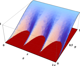
Figure 1: Plot showing the region of positivity when the initial pure state $\left|2\right\rangle$ is allowed to experience a uniform shrinking $(1-p)$ and rotation of angle $\theta$ by the matrix $f_{28}$ (see Appendix B). The quantity $1-3{\vec{n}}^{\prime}\cdot{\vec{n}}^{\prime}+2({\vec{n}}^{\prime}\star{\vec{n}}^{\prime})\cdot{\vec{n}}^{\prime}$ is graphed vertically since for this initial pure state the condition $1-3{\vec{n}}^{\prime}\cdot{\vec{n}}^{\prime}+2({\vec{n}}^{\prime}\star{\vec{n}}^{\prime})\cdot{\vec{n}}^{\prime}\geq 0$ is necessary and sufficient for positivity.

In Fig. 1 we plot the region of positivity as a function of the parameters $\theta$ and $p$. The figure shows that while $S_{3}=0$ initially $(p=\theta=0)$, this quantity quickly becomes negative as the state begins to rotate without shrinking. The figure also shows, although not very clearly, how the initial state becomes positive again as $\theta$ increases to multiples of $2\pi/3$ while no shrinking has occured. When the components of the initial coherence vector uniformily shrink by an amount $(1-p)>1/2$ we see that any rotation about the matrix $f_{28}$ leads to a positive density operator.

VIII Concluding Remarks

We have obtained an expression for an arbitrary affine mapping of the polarization vector associated with a $d$-dimensional density operator in terms of the components of the operator-sum representation of the dynamical map. This provides a geometric picture, albeit somewhat abstract, via the polarization vector components which are measurable quantities. We also described a direct method for expressing the affine map in terms of the dynamical map. Some example channels were provided in order to highlight the connection between particular terms in our expression and specific operators appearing in the OSR. For the important case that the OSR components are unitary and orthogonal, we have shown that the corresponding affine components are real and have trace -1 between pairs of unequal terms. This is particularly useful for the generalization of the Bloch equations since this basis is used for error prevention methods.

To generalize the methods used for qubit maps, we discussed the possible generalization of the singular value decomposition of qubit affine maps to higher dimensional systems. We have found that a symmetry-breaking occurs due to positivity constraints. Thus we have given a relation between the physical symmetry, the purity and the entropy of the physical system. In this particular case we have provided the example of the depolarizing channel, but the generalization is also discussed.

While we have provided some particular expressions for physically motivated quantum channels (maps), applications of this work range from information theory to practical experiments as is the case with the OSR. One example of the utility is given in Ref. Wu, L.-A. and Byrd, M.S. (2009), where the robust simulation of quantum systems with quantum systems was considered. In addition, the preferred basis given here provides a connection between quantum error correcting codes and direct application thereof. This is due, in part, to the ability to more directly determine the input and output, and therefore the map itself, for quantum systems undergoing noisy evolution. In future work we will use this to try to provide more practical methods for determining the best combination of error prevention methods. (See Byrd, M.S., Wu, L.-A. and Lidar, D.A. (2004) for a review.)

More generally, we anticipate applications of this could be more wide spread in quantum control. For example, classical control systems utilizing affine maps may be found in Judjevic’s book, “Geometric Control Theory,” chapter 4. This includes Linear systems reachability, and constraints. We also hope that our work will be useful in ways not yet foreseen by us.

Appendix A Identities

In this appendix we provide identities that were used in the derivations of the expressions above.

The commutation relations, anti-commutation relations, and normalization of the matrices representing the basis for the Lie algebra can be summarized by the following equation:

$$\lambda_{i}\lambda_{j}=\frac{2}{d}\delta_{ij}+if_{ijk}\lambda_{k}+d_{ijk}\lambda_{k},$$ (83)

where here, and throughout this appendix, a sum over repeated indices is understood.

As with any Lie algebra we have the Jacobi identity:

$$f_{ilm}f_{jkl}+f_{jlm}f_{kil}+f_{klm}f_{ijl}=0.$$ (84)

There is also a Jacobi-like identity,

$$f_{ilm}d_{jkl}+f_{jlm}d_{kil}+f_{klm}d_{ijl}=0,$$ (85)

which was given by Macfarlane, et al. A.J. Macfarlane, A. Sudbery and P.H. Weisz (1968).

The following identities, are also provided in A.J. Macfarlane, A. Sudbery and P.H. Weisz (1968),

$$d_{iik} = 0,$$ (86)

$$d_{ijk}f_{ljk} = 0,$$ (87)

$$f_{ijk}f_{ljk} = d\delta_{il},$$ (88)

$$d_{ijk}d_{ljk} = \frac{d^{2}-4}{d}\delta_{il},$$ (89)

and

$$f_{ijm}f_{klm}=\frac{2}{d}(\delta_{ik}\delta_{jl}-\delta_{il}\delta_{jk})+(d_{ikm}d_{jlm}-d_{jkm}d_{ilm})$$ (90)

and finally

$$f_{piq}f_{qjr}f_{rkp} = -\left(\frac{d}{2}\right)f_{ijk},$$ (91)

$$d_{piq}f_{qjr}f_{rkp} = -\left(\frac{d}{2}\right)d_{ijk},$$ (92)

$$d_{piq}d_{qjr}f_{rkp} = \left(\frac{d^{2}-4}{2d}\right)f_{ijk},$$ (93)

$$d_{piq}d_{qjr}d_{rkp} = \left(\frac{d^{2}-12}{2d}\right)d_{ijk}.$$ (94)

The proofs of these are fairly straight-forward and are omitted.

Appendix B Algebra of rotation matrices

In this section we provide the basis elements for the symmetry breaking from the SO(8) symmetry to the SU(3) symmetry. A basis for the algebra of SO(8) is given by one set of matrices and the SU(3) algebraic basis elements are expressed in terms of that basis using the structure constants which provide the algebra for the adjoint representation of the group. This provides the afforementioned embedding of the group SU(3) into SO(8) by the exponentiation of the algebra.

The structure constants for SU(3) are $f_{ijk}$ and we write them in matrix form as $(f_{i})_{jk}$, i.e. the matrix $f_{i}$ has elements $j,k$. Consider the basis for a matrix representation of SO(8) given by the set of all

$$m_{jk}=i(\left|j\right\rangle\!\!\left\langle k\right|-\left|k\right\rangle\!\!\left\langle j\right|),$$

for which $j<k=2,...,8$.

For SU(3) we label the matrices 1-8, with elements $j,k$ corresponding to the eight Gell-Mann matrices. The basis is

$$\begin{array}[]{cc}f_{1jk}=i\left(\begin{array}[]{cccccccc}0&0&0&0&0&0&0&0\\ 0&0&1&0&0&0&0&0\\ 0&-1&0&0&0&0&0&0\\ 0&0&0&0&0&0&\frac{1}{2}&0\\ 0&0&0&0&0&-\frac{1}{2}&0&0\\ 0&0&0&0&\frac{1}{2}&0&0&0\\ 0&0&0&-\frac{1}{2}&0&0&0&0\\ 0&0&0&0&0&0&0&0\end{array}\right)&f_{2jk}=i\left(\begin{array}[]{cccccccc}0&0&1&0&0&0&0&0\\ 0&0&0&0&0&0&0&0\\ -1&0&0&0&0&0&0&0\\ 0&0&0&0&0&\frac{1}{2}&0&0\\ 0&0&0&0&0&0&\frac{1}{2}&0\\ 0&0&0&-\frac{1}{2}&0&0&0&0\\ 0&0&0&0&-\frac{1}{2}&0&0&0\\ 0&0&0&0&0&0&0&0\end{array}\right)\\ f_{3jk}=i\left(\begin{array}[]{cccccccc}0&1&0&0&0&0&0&0\\ -1&0&0&0&0&0&0&0\\ 0&0&0&0&0&0&0&0\\ 0&0&0&0&\frac{1}{2}&0&0&0\\ 0&0&0&-\frac{1}{2}&0&0&0&0\\ 0&0&0&0&0&0&-\frac{1}{2}&0\\ 0&0&0&0&0&\frac{1}{2}&0&0\\ 0&0&0&0&0&0&0&0\end{array}\right)&f_{4jk}=i\left(\begin{array}[]{cccccccc}0&0&0&0&0&0&-\frac{1}{2}&0\\ 0&0&0&0&0&-\frac{1}{2}&0&0\\ 0&0&0&0&-\frac{1}{2}&0&0&0\\ 0&0&0&0&0&0&0&0\\ 0&0&\frac{1}{2}&0&0&0&0&\frac{\sqrt{3}}{2}\\ 0&\frac{1}{2}&0&0&0&0&0&0\\ \frac{1}{2}&0&0&0&0&0&0&0\\ 0&0&0&0&-\frac{\sqrt{3}}{2}&0&0&0\end{array}\right)\\ f_{5jk}=i\left(\begin{array}[]{cccccccc}0&0&0&0&0&\frac{1}{2}&0&0\\ 0&0&0&0&0&0&-\frac{1}{2}&0\\ 0&0&0&\frac{1}{2}&0&0&0&0\\ 0&0&-\frac{1}{2}&0&0&0&0&\frac{\sqrt{3}}{2}\\ 0&0&0&0&0&0&0&0\\ -\frac{1}{2}&0&0&0&0&0&0&0\\ 0&\frac{1}{2}&0&0&0&0&0&0\\ 0&0&0&\frac{\sqrt{3}}{2}&0&0&0&0\end{array}\right)&f_{6jk}=i\left(\begin{array}[]{cccccccc}0&0&0&0&-\frac{1}{2}&0&0&0\\ 0&0&0&-\frac{1}{2}&0&0&0&0\\ 0&0&0&0&0&0&\frac{1}{2}&0\\ 0&\frac{1}{2}&0&0&0&0&0&0\\ \frac{1}{2}&0&0&0&0&0&0&0\\ 0&0&0&0&0&0&0&0\\ 0&0&-\frac{1}{2}&0&0&0&0&\frac{\sqrt{3}}{2}\\ 0&0&0&0&0&0&-\frac{\sqrt{3}}{2}&0\end{array}\right)\\ f_{7jk}=i\left(\begin{array}[]{cccccccc}0&0&0&\frac{1}{2}&0&0&0&0\\ 0&0&0&0&\frac{1}{2}&0&0&0\\ 0&0&0&0&0&-\frac{1}{2}&0&0\\ -\frac{1}{2}&0&0&0&0&0&0&0\\ 0&-\frac{1}{2}&0&0&0&0&0&0\\ 0&0&\frac{1}{2}&0&0&0&0&-\frac{\sqrt{3}}{2}\\ 0&0&0&0&0&0&0&0\\ 0&0&0&0&0&\frac{\sqrt{3}}{2}&0&0\end{array}\right)&f_{8jk}=i\left(\begin{array}[]{cccccccc}0&0&0&0&0&0&0&0\\ 0&0&0&0&0&0&0&0\\ 0&0&0&0&0&0&0&0\\ 0&0&0&0&\frac{\sqrt{3}}{2}&0&0&0\\ 0&0&0&-\frac{\sqrt{3}}{2}&0&0&0&0\\ 0&0&0&0&0&0&\frac{\sqrt{3}}{2}&0\\ 0&0&0&0&0&-\frac{\sqrt{3}}{2}&0&0\\ 0&0&0&0&0&0&0&0\end{array}\right)\end{array}$$

These are clearly basis elements for the adjoint representation of the algebra which is a subset of the SO(8) algebra.

We now make the connection between the two by writing the basis elements for SU(3) in terms of the SO(8) basis elements.

$$f_{1} = m_{23}+\frac{1}{2}(m_{47}-m_{56}),\hskip 57.81621ptf_{2}=-m_{13}+\frac{1}{2}(m_{46}+m_{57})$$ (95)

$$f_{3} = m_{12}+\frac{1}{2}(m_{45}-m_{67}),\hskip 57.81621ptf_{4}=-\frac{1}{2}(m_{17}+m_{26}+m_{35})+\frac{\sqrt{3}}{2}m_{58}$$ (96)

$$f_{5} = \frac{1}{2}(m_{16}-m_{27}+m_{34})-\frac{\sqrt{3}}{2}m_{48},\;\;\;\;f_{6}=\frac{1}{2}(-m_{15}+m_{24}+m_{37})+\frac{\sqrt{3}}{2}m_{78}$$ (97)

$$f_{7} = \frac{1}{2}(m_{14}+m_{25}-m_{36})-\frac{\sqrt{3}}{2}m_{68},\hskip 14.45377ptf_{8}=\frac{\sqrt{3}}{2}(m_{45}+m_{67})$$ (98)

Let us now complete the basis by finding a complete set of 28 matrices which are orthogonal in the Hilbert-Schmidt sense and have $f_{i},\;i=1,...,8$ as members. Considering the Hilbert-Schmidt to be an inner product, we can immediately write down a complete set. We will number them in no particular order. (IMPORTANT: We will also assume for now that they are normalized such that Tr$(m_{ij}m_{kl})=\delta_{ik}\delta_{jl}$. This can be adjusted later if it is not true.) Let us consider a set of matrices which span the space $m_{23},m_{47},m_{56}$ when $f_{1}$ is included. The set is (for $f_{1}$)

$$f_{9}=\frac{1}{2}(m_{47}+m_{56}),\;\;f_{10}=-(m_{47}-m_{56}).$$

Similarly, we will group the remaining matrices: ($f_{2}$)

$$f_{11}=m_{13}+(m_{46}+m_{57}),\;\;f_{12}=(m_{46}-m_{57}),$$

($f_{3}$ and $f_{8}$)

$$f_{13}=m_{12}-(m_{45}-m_{67}),$$

($f_{4}$)

$$f_{14}=(m_{17}+m_{26}+m_{35})+\sqrt{3}\;m_{58},\;\;f_{15}=m_{17}-2m_{26}+m_{35},\;\;f_{16}=m_{17}-m_{35}$$

($f_{5}$)

$$f_{17}=(m_{16}-m_{27}+m_{34})+\sqrt{3}\;m_{48},\;\;f_{18}=m_{16}+2m_{27}+m_{34},\;\;f_{19}=m_{16}-m_{34}$$

($f_{6}$)

$$f_{20}=(-m_{15}+m_{24}+m_{37})-\sqrt{3}\;m_{78},\;\;f_{21}=m_{24}+2m_{15}+m_{37},\;\;f_{22}=m_{24}-m_{37}$$

($f_{7}$)

$$f_{23}=(m_{14}+m_{25}-m_{36})+\sqrt{3}\;m_{68},\;\;f_{24}=m_{14}+2m_{36}+m_{25},\;\;f_{25}=m_{14}-m_{25}.$$

Finally, we have the following three:

$$f_{26}=m_{18},\;\;f_{27}=m_{28},\;\;f_{28}=m_{38}.$$

References

- A. Peres (1996) A. Peres, Phys. Rev. Lett. 77, 1413 (1996).
- M. Horodecki, P. Horodecki and R. Horodecki (1996) M. Horodecki, P. Horodecki and R. Horodecki, Phys. Lett. A 223, 1 (1996).
- E. C. G. Sudarshan, P. M. Mathews and J. Rau (1961) E. C. G. Sudarshan, P. M. Mathews and J. Rau, Phys. Rev. 121, 920 (1961).
- K. Kraus (1983) K. Kraus, States, Effects and Operations, Fundamental Notions of Quantum Theory (Academic, Berlin, 1983).
- P. Pechukas (1994) P. Pechukas, Phys. Rev. Lett. 73, 1060 (1994).
- (6) R. Alicki, Phys. Rev. Lett. 75, 3020 (1995); P. Pechukas, ibid., p. 3021.
- T.F. Jordan, A. Shaji and E. C. G. Sudarshan (2004) T.F. Jordan, A. Shaji and E. C. G. Sudarshan, Phys. Rev. A 70, 052110 (2004).
- A. Shaji and E.C.G. Sudarshan (2005) A. Shaji and E.C.G. Sudarshan, Phys. Lett. A 341, 48 (2005).
- Shabani and Lidar (2009a) A. Shabani and D. A. Lidar, Phys. Rev. Lett. 102, 100402 (2009a).
- Rodríguez-Rosario et al. (2010) C. A. Rodríguez-Rosario, K. Modi, and A. Aspuru-Guzik, Phys. Rev. A 81, 012313 (2010).
- Shabani and Lidar (2009b) A. Shabani and D. Lidar, Phys. Rev. A 80, 012309 (2009b).
- D. Dong and I.R. Petersen (2009) D. Dong and I.R. Petersen (2009), arXiv:0910.2350.
- C. Brif, R. Chakrabarti, H. Rabitz (2010) C. Brif, R. Chakrabarti, H. Rabitz, New J. Phys. 12, 075008 (2010).
- Nielsen and Chuang (2000) M. Nielsen and I. Chuang, Quantum Computation and Quantum Information (Cambridge University Press, 2000).
- C. King and M.B. Ruskai (2001) C. King and M.B. Ruskai, IEEE Trans. Info. Th. 47, 192 (2001).
- Mahler, G. and Weberruss, V.A. (1998) Mahler, G. and Weberruss, V.A., Quantum Networks: Dynamics of Open Nanostructures (Springer Verlag, Berlin, 1998), 2nd ed.
- L. Jakóbczyk and M. Siennicki (2001) L. Jakóbczyk and M. Siennicki, Phys. Lett. A 286, 383 (2001).
- Arvind, K. S. Mallesh and N. Mukunda (1997) Arvind, K. S. Mallesh and N. Mukunda, J. Phys. A 30, 2417 (1997).
- Byrd, M.S. and N. Khaneja (2003) Byrd, M.S. and N. Khaneja, Phys. Rev. A 68, 062322 (2003).
- G. Kimura (2003) G. Kimura, Phys. Lett. A 314, 339 (2003).
- G. Kimura and A. Kossakowski (2005) G. Kimura and A. Kossakowski, Open Sys. & Information Dyn. 12, 207 (2005).
- (22) We note that the final form is a generalized version of what is now sometimes called a Kraus decomposition. Kraus took up the study of such maps in the early 1970s and published the often-cited set of lecture notes K. Kraus (1983).
- Byrd, M.S. (1998) Byrd, M.S., J. Math. Phys. 39, 6125 (1998).
- Ou, Y.-C. and Byrd, M.S. (2010) Ou, Y.-C. and Byrd, M.S., Phys. Rev. A 82, 022325 (2010).
- A. Checinska, K. Wodkiewicz (2008) A. Checinska, K. Wodkiewicz (2008), arXiv:0809.3882.
- Byrd, M.S., Brennen, G.K. (2008) Byrd, M.S., Brennen, G.K., Phys. Lett. A 372, 1770 (2008).
- Knill (1996) E. Knill (1996), lANL ePrint quant-ph/9608049.
- (28) Ou, Y.-C. and Byrd, M.B., Pseudo-Unitary Freedom for General Maps, in progress.
- Bishop, C.A. and Byrd, M.S. (2009) Bishop, C.A. and Byrd, M.S., J. Phys. A: Math. Theor. 42, 055301 (2009).
- Fujiwara and Algoet (1999) A. Fujiwara and P. Algoet, Phys. Rev. A 59, 3290 (1999).
- A. Bohm (1993) A. Bohm, Quantum Mechanics: Foundations and Applications, 3rd Ed., Chapter 5 (Springer-Verlag, New York, New York, 1993).
- Wu, L.-A. and Byrd, M.S. (2009) Wu, L.-A. and Byrd, M.S., Qu. Inf. Proc. 8 (2009).
- Byrd, M.S., Wu, L.-A. and Lidar, D.A. (2004) Byrd, M.S., Wu, L.-A. and Lidar, D.A., J. Mod. Optics 51, 2449 (2004).
- A.J. Macfarlane, A. Sudbery and P.H. Weisz (1968) A.J. Macfarlane, A. Sudbery and P.H. Weisz, Commun. Math. Phys. 11, 77 (1968).