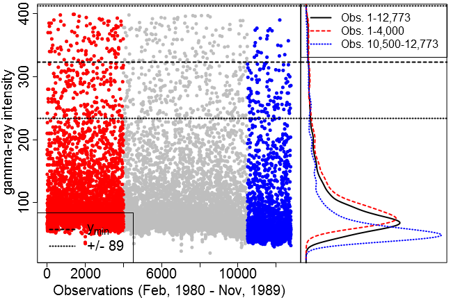
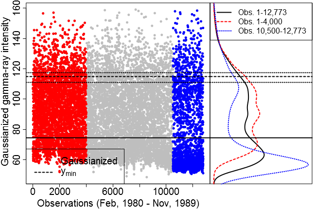
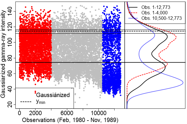
The Lambert Way to Gaussianize heavy tailed data with the inverse of Tukey’s h transformation as a special case

Georg M. Goerg Department of Statistics, Carnegie Mellon University
Pittsburgh, PA 15213, USA
gmg@stat.cmu.edu, www.stat.cmu.edu/~gmg

I present a parametric, bijective transformation to generate heavy tail versions Y𝑌Y of arbitrary RVs XFXsimilar-to𝑋subscript𝐹𝑋X\sim F_{X}. The tail behavior of the so-called heavy tail Lambert W ×\times FXsubscript𝐹𝑋F_{X} RV Y𝑌Y depends on a tail parameter δ0𝛿0\delta\geq 0: for δ=0𝛿0\delta=0, YX𝑌𝑋Y\equiv X, for δ>0𝛿0\delta>0 Y𝑌Y has heavier tails than X𝑋X. For X𝑋X being Gaussian, this meta-family of heavy-tailed distributions reduces to Tukey’s hh distribution. Lambert’s W𝑊W function provides an explicit inverse transformation, which can be estimated by maximum likelihood. This inverse can remove heavy tails from data, and also provide analytical expressions for the cumulative distribution (cdf) and probability density function (pdf). As a special case, these yield explicit formulas for Tukey’s hh pdf and cdf - to the author’s knowledge for the first time in the literature. Simulations and applications to S&P 500 log-returns and solar flares data demonstrate the usefulness of the introduced methodology.

The R package LambertW implementing the presented methodology is publicly available at CRAN.

1 Introduction

Statistical theory and practice are both tightly linked to Gaussianity. In theory, many methods require Gaussian data or noise: i) regression often assumes Gaussian errors; ii) pattern recognition for images often model noise as a Gaussian random field (Achim et al., 2003); iii) many time series models are based on Gaussian white noise (Brockwell and Davis, 1998; Engle, 1982; Granger and Joyeux, 2001).

In all these cases, a model 𝒩subscript𝒩\mathcal{M}_{\mathcal{N}}, parameter estimates and their standard errors, and other properties, are then studied – all based on the ideal(istic) assumption of Gaussianity.

In practice, however, data/noise often exhibits asymmetry and heavy tails; for example wind speed data (Field, 2004), human dynamics

(Vázquez et al., 2006), or Internet traffic data (Gidlund and Debernardi, 2009) – just to a name few. Particularly notable examples are financial data (Cont, 2001; Kim and White, 2003) and speech signals (Aysal and Barner, 2006), which almost exclusively exhibit heavy tails. Thus a model 𝒩subscript𝒩\mathcal{M}_{\mathcal{N}} developed for the Gaussian case does not necessarily provide accurate inference anymore.

One way to overcome this shortcoming is to replace 𝒩subscript𝒩\mathcal{M}_{\mathcal{N}} with a new model Gsubscript𝐺\mathcal{M}_{G}, where G𝐺G is a heavy tail distribution: i) regression with Cauchy errors (Smith, 1973); ii) image denoising for α𝛼\alpha-stable noise (Achim et al., 2003); iii) forecasting long memory processes with heavy tail innovations (Ilow, 2000; Palma and Zevallos, 2011), or ARMA modeling of electricity loads with hyperbolic noise (Nowicka-Zagrajek and Weron, 2002).

While such fundamental approaches are attractive from a theoretical perspective, they can become unsatisfactory from a practical viewpoint. Many successful statistical models assume Gaussianity, their theory is very well understood, and many algorithms are implemented for the simple – and often much faster – Gaussian case. Thus developing models based on an entirely unrelated distribution G𝐺G is like throwing out the (Gaussian) baby with the bathwater.

It would be very useful to transform a Gaussian RV X𝑋X to a heavy-tailed RV Y𝑌Y and vice versa, and thus rely on knowledge - and software - for the well-understood Gaussian case, while still capturing heavy tails in the data. Optimally such a transformation should: a) be bijective; b) include Normality as a special case for hypothesis testing; and c) be parametric so the optimal transformation can be estimated efficiently.

X𝑋X and 𝐱𝐱\mathbf{x} Hτ(X)subscript𝐻𝜏𝑋H_{\tau}(X) Y𝑌Y and 𝐲𝐲\mathbf{y}Xτsubscript𝑋𝜏X_{\tau} and 𝐱τsubscript𝐱𝜏\mathbf{x}_{\tau}Wτ(Y)=Hτ1(Y)subscript𝑊𝜏𝑌subscriptsuperscript𝐻1𝜏𝑌W_{\tau}(Y)=H^{-1}_{\tau}(Y)FXsubscript𝐹𝑋F_{X} and FXτsubscript𝐹subscript𝑋𝜏F_{X_{\tau}}
Lambert W ×\times FXsubscript𝐹𝑋F_{X}
(Tukey’s hh if FX=𝒩subscript𝐹𝑋𝒩F_{X}=\mathcal{N})
inference
on Y𝑌Y
inference
on Xτsubscript𝑋𝜏X_{\tau}
Hτ()subscript𝐻𝜏H_{\tau}(\cdot) latent (Gaussian) observed (heavy tails) recovered “Gaussianize” heavy tails
methods/models
assuming
Gaussianity
exact
methods/models
for heavy-tailed
distributions (if \exists)
approx.
Figure 1: Schematic view of the heavy tail Lambert W ×\times FXsubscript𝐹𝑋F_{X} framework. (left) Latent input XFXsimilar-to𝑋subscript𝐹𝑋X\sim F_{X}: Hτ(X)subscript𝐻𝜏𝑋H_{\tau}(X) from (6) transforms (solid arrows) X𝑋X to Ysimilar-to𝑌absentY\sim Lambert W ×\times FXsubscript𝐹𝑋F_{X} and generates heavy tails. (right) Observed heavy tail world Y𝑌Y and 𝐲𝐲\mathbf{y}: (1) use Wτ()subscript𝑊𝜏W_{\tau}(\cdot) to back-transform 𝐲𝐲\mathbf{y} to latent “Normal” 𝐱τsubscript𝐱𝜏\mathbf{x}_{\tau}, (2) use model 𝒩subscript𝒩\mathcal{M}_{\mathcal{N}} of your choice (regression, time series models, hypothesis testing, etc.) for inference on 𝐱τsubscript𝐱𝜏\mathbf{x}_{\tau}, and (3) convert results back to the original “heavy-tailed world” of 𝐲𝐲\mathbf{y}.

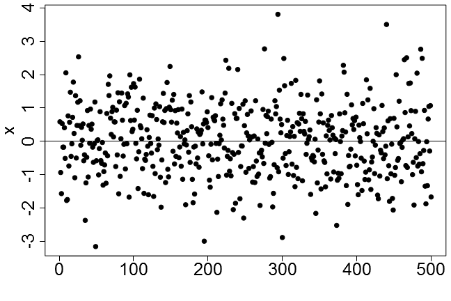
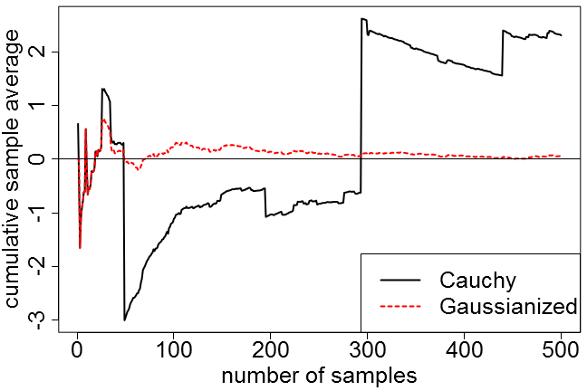
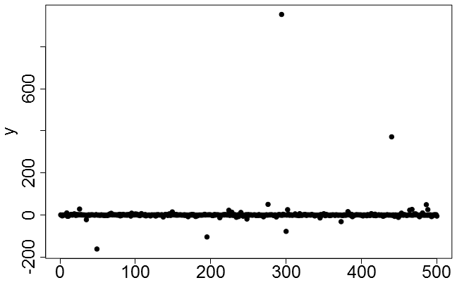
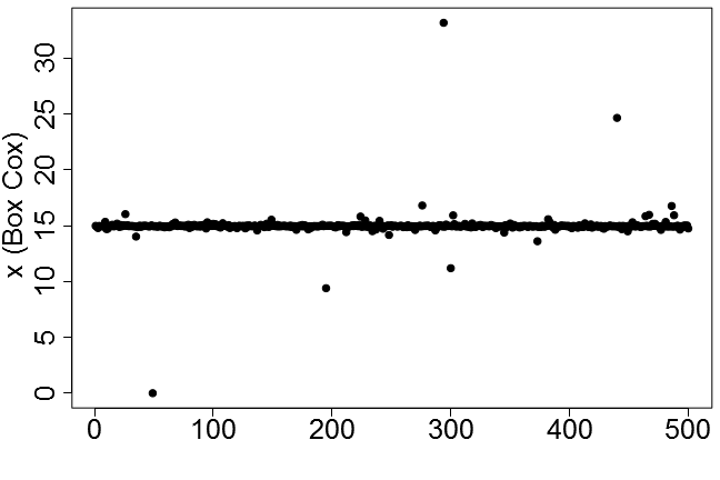
Figure 1 illustrates this pragmatic approach: researchers can make their observations 𝐲𝐲\mathbf{y} as Gaussian as possible (𝐱τsubscript𝐱𝜏\mathbf{x}_{\tau}) before making inference based on their favorite Gaussian model 𝒩subscript𝒩\mathcal{M}_{\mathcal{N}}. This avoids the development of - or the data analysts waiting for - a whole new theory of Gsubscript𝐺\mathcal{M}_{G} and new implementations based on a particular heavy-tailed distribution G𝐺G, while still improving statistical inference on heavy-tailed data 𝐲𝐲\mathbf{y}. For example, consider 𝐲=(y1,,y500)𝐲subscript𝑦1subscript𝑦500\mathbf{y}=(y_{1},\ldots,y_{500}) from a standard Cauchy distribution 𝒞(0,1)𝒞01\mathcal{C}(0,1) in Fig. 2a: modeling heavy tails by a transformation makes it even possible to Gaussianize this Cauchy sample (Fig. 2c). This “nice” data 𝐱τsubscript𝐱𝜏\mathbf{x}_{\tau} can then be subsequently analyzed with common techniques. For example, the location can now be estimated using the sample average (Fig. 2d). For details see Section 6.1.

Liu et al. (2009) use a semi-parametric approach, where Y𝑌Y has a nonparanormal distribution if f(Y)𝒩(μ,σ2)similar-to𝑓𝑌𝒩𝜇superscript𝜎2f(Y)\sim\mathcal{N}(\mu,\sigma^{2}) where f()𝑓f(\cdot) is an increasing smooth function; they estimate f()𝑓f(\cdot) using non-parametric methods. This leads to a greater flexibility in the distribution of Y𝑌Y, but it suffers from two drawbacks: i) non-parametric methods have slower convergence rates and thus need large samples, and ii) for identifiability of f()𝑓f(\cdot), 𝔼f(Y)𝔼Y𝔼𝑓𝑌𝔼𝑌\mathbb{E}f(Y)\equiv\mathbb{E}Y and 𝕍f(Y)𝕍Y𝕍𝑓𝑌𝕍𝑌\mathbb{V}f(Y)\equiv\mathbb{V}Y must hold. While i) is inherent to non-parametric methods, point ii) requires Y𝑌Y to have finite mean and variance, which is especially limiting for heavy-tailed data where this condition is often not met. Thus here we use parametric transformations which do not rely on restrictive identifiability conditions and also work well for small sample sizes.

The main contributions of this work are three-fold: a) following Goerg (2011) I introduce a meta-family of heavy tail Lambert W ×\times FXsubscript𝐹𝑋F_{X} distributions with Tukey’s hh (Hoaglin, 2006) as a special case; b) I present a bijective transformation to “Gaussianize” heavy-tailed data (Section 2); and c) I also provide simple expressions for the cumulative distribution function (cdf) GY(y)subscript𝐺𝑌𝑦G_{Y}(y) and probability density function (pdf) gY(y)subscript𝑔𝑌𝑦g_{Y}(y) - also for Tukey’s hh –, which can be easily implemented in statistics software (Section 2.4).

To the author’s knowledge analytic expressions for Tukey’s hh cdf and pdf are presented here (Section 3) for the first time in the literature. Section 4 introduces a methods of moments estimator and studies the maximum likelihood estimator (MLE). Section 5 shows their finite sample properties.

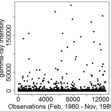
As has been shown in many case studies, Tukey’s hh distribution (heavy tail Lambert W ×\times Gaussian) is useful to model data with unimodal, heavy-tailed densities. Section 6 not only confirms this finding for S&P 500 log-returns, but also demonstrates the benefits of removing heavy tails for exploratory data analysis: Gaussianizing γ𝛾\gamma-ray intensity data reveals a bimodal density, which even non-parametric estimators fail to detect if heavy tails are not removed. Finally, we discuss the new methodology and future work in Section 7. All proofs are given in the Supplementary Material, Appendix B.

Computations, figures, and simulations were done in R (R Development Core Team, 2010). The R package LambertW is publicly available on CRAN.
Refer to caption
(a) Random sample 𝐲𝒞(0,1)similar-to𝐲𝒞01\mathbf{y}\sim\mathcal{C}(0,1)
Refer to caption
(b) Box-Cox transformed 𝐱λ^MLEsubscript𝐱subscript^𝜆𝑀𝐿𝐸\mathbf{x}_{\widehat{\lambda}_{MLE}} with λ^=0.37^𝜆0.37\widehat{\lambda}=0.37
Refer to caption
(c) Gaussianized 𝐱τ^MLEsubscript𝐱subscript^𝜏𝑀𝐿𝐸\mathbf{x}_{\widehat{\tau}_{MLE}} with τ^=(0.03,1.05,0.86)^𝜏0.031.050.86\widehat{\tau}=(0.03,1.05,0.86)
Refer to caption
(d) Cumulative sample average
Figure 2: Gaussianizing a standard Cauchy sample. For (d) τ(n)superscript𝜏𝑛\tau^{(n)} was estimated for each fixed n=5,,500𝑛5500n=5,\ldots,500, before Gaussianizing (y1,,yn)subscript𝑦1subscript𝑦𝑛(y_{1},\ldots,y_{n}).

1.1 Multivariate Extensions

While this work focuses on univariate case, multivariate extensions of the presented methods can be defined component-wise – analogously to the multivariate version of Tukey’s hh distribution (Field and Genton, 2006). While this may not make the transformed RVs jointly Gaussian, it still provides a good starting point for more well-behaved multivariate modeling.

1.2 Box-Cox Transformation to Remove Heavy Tails

A popular method to deal with skewed, high variance data is the Box-Cox transformation

𝐲λ={𝐲λ1λ if λ>0log𝐲 if λ=0.subscript𝐲𝜆casessuperscript𝐲𝜆1𝜆 if 𝜆0𝐲 if 𝜆0\mathbf{y}_{\lambda}=\begin{cases}\frac{\mathbf{y}^{\lambda}-1}{\lambda}&\text{ if }\lambda>0\\ \log\mathbf{y}&\text{ if }\lambda=0.\end{cases} (1)

The parameter λ𝜆\lambda can be chosen by MLE. However one major limitation of (1) is the non-negativity constraint on 𝐲𝐲\mathbf{y}, which prohibits its use in many applications. To avoid this limitation it is common to shift the data, 𝐲~=𝐲+|min(𝐲)|0~𝐲𝐲𝐲0\tilde{\mathbf{y}}=\mathbf{y}+|\min(\mathbf{y})|\geq 0. However, as Fig. 2b shows applying the Box-Cox transformation to the Cauchy sample111We use 𝐲~=𝐲+|min(𝐲)|+1~𝐲𝐲𝐲1\tilde{\mathbf{y}}=\mathbf{y}+|\min(\mathbf{y})|+1 and use boxcox from the MASS R package; λ^=0.37^𝜆0.37\widehat{\lambda}=0.37. completely fails. Furthermore, this restricts Y𝑌Y to a half-open interval [c,)𝑐[c,\infty) and is not desirable if the underlying process can occur on the entire real line, since it undermines statistical inference for yet unobserved data. See Sakia (1992) for a more detailed discussion and the Box-Cox transformation in general.

Furthermore, the main purpose of the Box-Cox transformation is to stabilize variance (Blaylock et al., 1980; Lawrance, 1987; Tsiotas, 2007) and remove right tail skewness (Goncalves and Meddahi, 2011); a lower empirical kurtosis is merely a by-result of the variance stabilization. In contrast, the Lambert W framework is designed to model heavy-tailed RVs and remove heavy tails from data, and has no difficulties with negative values.

2 Generating Heavy Tails Using Transformations

Random variables exhibit heavy tails if more mass than for a Gaussian RV lies at the outer end of the density support. A RV Z𝑍Z has a tail index a𝑎a if its cdf satisfies 1FZ(z)L(z)zasimilar-to1subscript𝐹𝑍𝑧𝐿𝑧superscript𝑧𝑎1-F_{Z}(z)\sim L(z)z^{-a}, where L(z)𝐿𝑧L(z) is a slowly varying function at infinity, i.e. limzL(tz)L(z)=1subscript𝑧𝐿𝑡𝑧𝐿𝑧1\lim_{z\rightarrow\infty}\frac{L(tz)}{L(z)}=1 for all t>0𝑡0t>0 (Baek and Pipiras, 2010).222There are various similar definitions of heavy/fat/long tails; for this work these differences are not essential. The heavy tail index a𝑎a is an important characteristic of Z𝑍Z; for example, only moments up to order a𝑎a exist.

2.1 Tukey’s hh Distribution

A parametric transformation is the basis of Tukey’s hh RVs (Hoaglin, 2006)

Z=Uexp(h2U2),h0,formulae-sequence𝑍𝑈2superscript𝑈20Z=U\exp\left(\frac{h}{2}U^{2}\right),\quad h\geq 0, (2)

where U𝑈U is standard Normal RV and hh is the heavy tail parameter. The RV Z𝑍Z has tail parameter a=1/h𝑎1a=1/h (Morgenthaler and Tukey, 2000) and reduces to the Gaussian for h=00h=0. Morgenthaler and Tukey (2000) extend the hh distribution to the skewed, heavy-tailed family of hhhh RVs

Z={Uexp(δ2U2),if U0,Uexp(δr2U2),if U>0,𝑍cases𝑈subscript𝛿2superscript𝑈2if 𝑈0𝑈subscript𝛿𝑟2superscript𝑈2if 𝑈0Z=\begin{cases}U\exp\left(\frac{\delta_{\ell}}{2}U^{2}\right),&\text{if }U\leq 0,\\ U\exp\left(\frac{\delta_{r}}{2}U^{2}\right),&\text{if }U>0,\end{cases} (3)

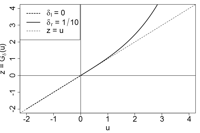
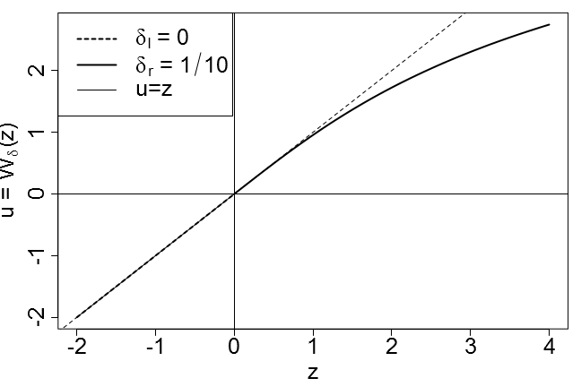
where again U𝒩(0,1)similar-to𝑈𝒩01U\sim\mathcal{N}(0,1). Here δ0subscript𝛿0\delta_{\ell}\geq 0 and δr0subscript𝛿𝑟0\delta_{r}\geq 0 shape the left and right tail of Z𝑍Z, respectively; thus transformation (3) can model skewed and heavy-tailed data - see Fig. 3a. For simplicity let Hδ(u):=uexp(δ2u2)assignsubscript𝐻𝛿𝑢𝑢𝛿2superscript𝑢2H_{\delta}(u):=u\exp\left(\frac{\delta}{2}u^{2}\right).

Refer to caption
(a) δδrsubscript𝛿subscript𝛿𝑟\delta_{\ell}\delta_{r} transformation (3)
Refer to caption
(b) Inverse Wδ,δr(z)subscript𝑊subscript𝛿subscript𝛿𝑟𝑧W_{\delta_{\ell},\delta_{r}}(z) in (10)
Refer to caption
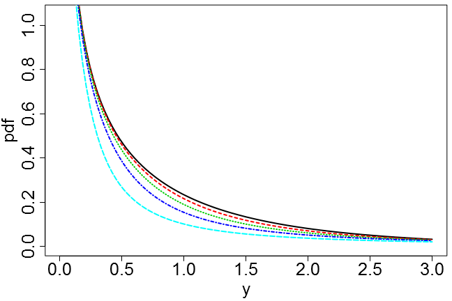
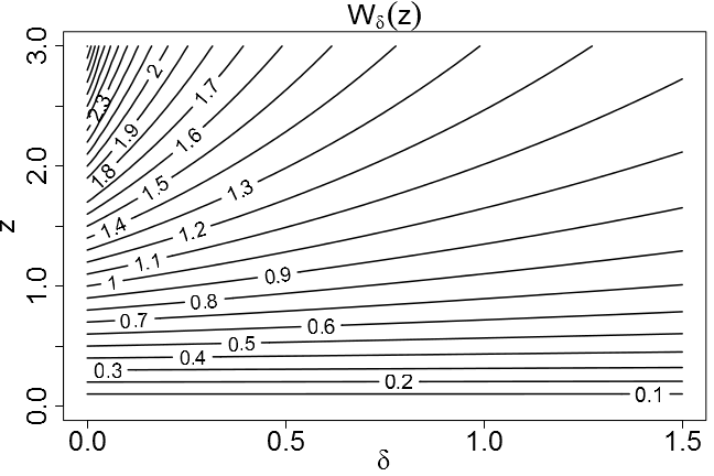
(c) Inverse Wδ(z)subscript𝑊𝛿𝑧W_{\delta}(z) (9) as a function of δ𝛿\delta and z𝑧z
Figure 3: Transformation and inverse transformation for δ=0subscript𝛿0\delta_{\ell}=0 and δr=1/10subscript𝛿𝑟110\delta_{r}=1/10: identity on the left (same tail behavior) and a heavy-tailed transformation in the right tail of input U𝑈U.

Despite their great flexibility they are not popular in statistical practice, because the inverse of (2) or (3) has not been found. Consequently, no closed-form expressions for the cdf or pdf are available. Although Morgenthaler and Tukey (2000) express the pdf of (2) as (hδ𝛿h\equiv\delta)

gZ(z)=fU(Hδ1(z))Hδ(Hδ1(z)),subscript𝑔𝑍𝑧subscript𝑓𝑈superscriptsubscript𝐻𝛿1𝑧superscriptsubscript𝐻𝛿superscriptsubscript𝐻𝛿1𝑧g_{Z}(z)=\frac{f_{U}\left(H_{\delta}^{-1}(z)\right)}{H_{\delta}^{{}^{\prime}}\left(H_{\delta}^{-1}(z)\right)}, (4)

they fall short of explicitly specifying Hδ1(z)superscriptsubscript𝐻𝛿1𝑧H_{\delta}^{-1}(z). So far this inverse has been considered analytically intractable (Field, 2004), or was only numerically approximated (Headrick et al., 2008; Fischer, 2010). Thus parameter inference relied on matching empirical and theoretical quantiles (Field, 2004; Morgenthaler and Tukey, 2000), or by the method of moments (Headrick et al., 2008). Only recently Headrick et al. (2008) provided numerical approximations. Hence, a closed form, analytically tractable pdf that can be computed efficiently is essential for a wide-spread use of Tukey’s hh (& variants).

In this work I present this long sought explicit inverse, which is readily available in standard statistics software. For ease of notation and concision main results are shown for δ=δr=δsubscript𝛿subscript𝛿𝑟𝛿\delta_{\ell}=\delta_{r}=\delta; analogous results for δδrsubscript𝛿subscript𝛿𝑟\delta_{\ell}\neq\delta_{r} will be stated without details.

2.2 Heavy Tail Lambert W Random Variables

Tukey’s hh transformation (2) is strongly related to the approach taken by Goerg (2011) to introduce skewness in continuous RVs XFX(x)similar-to𝑋subscript𝐹𝑋𝑥X\sim F_{X}(x). In particular, if Zsimilar-to𝑍absentZ\sim Tukey’s hh, then Z2similar-tosuperscript𝑍2absentZ^{2}\sim skewed Lambert W ×χ12absentsubscriptsuperscript𝜒21\times\chi^{2}_{1} with skew parameter γ=h𝛾\gamma=h.

Adapting the skew Lambert W ×\times FXsubscript𝐹𝑋F_{X} input/output idea333Most concepts and methods from the skew Lambert W ×FXabsentsubscript𝐹𝑋\times F_{X} case transfer one-to-one to the heavy tail Lambert W RVs presented here. Thus for the sake of concision I refer to Goerg (2011) for details and background information on the Lambert W framework. (see Fig. 1), Tukey’s hh RVs can be generalized to heavy-tailed Lambert W ×\times FXsubscript𝐹𝑋F_{X} RVs.

Definition 2.1.

Let U𝑈U be a continuous RV with cdf FU(u𝛃)subscript𝐹𝑈conditional𝑢𝛃F_{U}\left(u\mid\boldsymbol{\beta}\right), pdf fU(u𝛃)subscript𝑓𝑈conditional𝑢𝛃f_{U}\left(u\mid\boldsymbol{\beta}\right), and parameter vector 𝛃𝛃\boldsymbol{\beta}. Then,

Z=Uexp(δ2U2),δ,formulae-sequence𝑍𝑈𝛿2superscript𝑈2𝛿Z=U\exp\left(\frac{\delta}{2}U^{2}\right),\quad\delta\in\mathbb{R}, (5)

is a non-central, non-scaled heavy tail Lambert W ×\times FXsubscript𝐹𝑋F_{X} RV with parameter vector θ=(𝛃,δ)𝜃𝛃𝛿\theta=\left(\boldsymbol{\beta},\delta\right), where δ𝛿\delta is the tail parameter.

Tukey’s hh distribution results for U𝑈U being a standard Gaussian 𝒩(0,1)𝒩01\mathcal{N}(0,1).

Definition 2.2.

For a continuous location-scale family RV XFX(x𝛃)similar-to𝑋subscript𝐹𝑋conditional𝑥𝛃X\sim F_{X}(x\mid\boldsymbol{\beta}) define a location-scale heavy-tailed Lambert W ×\times FXsubscript𝐹𝑋F_{X} RV

Y={Uexp(δ2U2)}σx+μx,δ,formulae-sequence𝑌𝑈𝛿2superscript𝑈2subscript𝜎𝑥subscript𝜇𝑥𝛿Y=\left\{U\exp\left(\frac{\delta}{2}U^{2}\right)\right\}\sigma_{x}+\mu_{x},\quad\delta\in\mathbb{R}, (6)

with parameter vector θ=(𝛃,δ)𝜃𝛃𝛿\theta=(\boldsymbol{\beta},\delta), where U=(Xμx)/σx𝑈𝑋subscript𝜇𝑥subscript𝜎𝑥U=(X-\mu_{x})/\sigma_{x}.

The input is not necessarily Gaussian but can be any other location-scale continuous RV, e.g., from a uniform distribution: XU(a,b)similar-to𝑋𝑈𝑎𝑏X\sim U(a,b).

Definition 2.3.

Let XFX(x/s𝛃)similar-to𝑋subscript𝐹𝑋conditional𝑥𝑠𝛃X\sim F_{X}(x/s\mid\boldsymbol{\beta}) be a continuous scale-family RV, with standard deviation σxsubscript𝜎𝑥\sigma_{x}; let U=X/σx𝑈𝑋subscript𝜎𝑥U=X/\sigma_{x}. Then,

Y=Xexp(δ2U2),δ,formulae-sequence𝑌𝑋𝛿2superscript𝑈2𝛿Y=X\exp\left(\frac{\delta}{2}U^{2}\right),\quad\delta\in\mathbb{R}, (7)

is a scaled heavy-tailed Lambert W ×\times FXsubscript𝐹𝑋F_{X} RV with parameter θ=(𝛃,δ)𝜃𝛃𝛿\theta=\left(\boldsymbol{\beta},\delta\right).

Let τ:=(μx(𝜷),σx(𝜷),δ)assign𝜏subscript𝜇𝑥𝜷subscript𝜎𝑥𝜷𝛿\tau:=\left(\mu_{x}(\boldsymbol{\beta}),\sigma_{x}(\boldsymbol{\beta}),\delta\right) define transformation (6).444For non-central, non-scale input set τ=(0,1,δ)𝜏01𝛿\tau=(0,1,\delta); for scale-family input τ=(0,σx,δ)𝜏0subscript𝜎𝑥𝛿\tau=(0,\sigma_{x},\delta). If X(,)𝑋X\in(-\infty,\infty), then for all δ0𝛿0\delta\geq 0 also the location-scale Y(,)𝑌Y\in(-\infty,\infty). For a scale family X[0,)𝑋0X\in[0,\infty) also the scale Lambert W ×\times FXsubscript𝐹𝑋F_{X} RV Y[0,)𝑌0Y\in[0,\infty).

The shape parameter δ𝛿\delta (== Tukey’s hh) governs the tail behavior of Y𝑌Y: for δ>0𝛿0\delta>0 values further away from μxsubscript𝜇𝑥\mu_{x} are increasingly emphasized, leading to a heavy-tailed version of FX(x)subscript𝐹𝑋𝑥F_{X}(x); for δ=0𝛿0\delta=0, YX𝑌𝑋Y\equiv X; and for δ<0𝛿0\delta<0 values far away from the mean are mapped back again closer to μxsubscript𝜇𝑥\mu_{x}. Thus heavy tail Lambert W ×\times FXsubscript𝐹𝑋F_{X} RVs generalize XFX(x)similar-to𝑋subscript𝐹𝑋𝑥X\sim F_{X}(x) to heavy-tailed versions of itself, YGY(y)similar-to𝑌subscript𝐺𝑌𝑦Y\sim G_{Y}(y), with a reduction to X𝑋X for δ=0𝛿0\delta=0.

The Lambert W formulation of heavy tail modeling is more general than Tukey’s hh distribution as X𝑋X can have any distribution FX(x)subscript𝐹𝑋𝑥F_{X}(x), not necessarily Gaussian (Fig. 4).

Remark 2.4 (Only non-negative δ𝛿\delta).

Although δ<0𝛿0\delta<0 leads to interesting properties of Y𝑌Y, it yields a non-bijective transformation and thus to parameter-dependent support and non-unique input. Thus for the remainder of this work I tacitly assume δ0𝛿0\delta\geq 0, unless stated otherwise.

2.3 Inverse Transformation: “Gaussianize” Heavy-Tailed Data

Transformation (6) is bijective and its inverse can be obtained via Lambert’s W𝑊W function, which is the inverse of z=uexp(u)𝑧𝑢𝑢z=u\exp(u), i.e., that function which satisfies W(z)exp(W(z))=z𝑊𝑧𝑊𝑧𝑧W(z)\exp(W(z))=z. Lambert’s W𝑊W has been studied extensively in mathematics, physics, and other areas of science (Rosenlicht, 1969; Corless et al., 1996; Valluri et al., 2000), and is implemented in the GNU Scientific Library (GSL) (Galassi et al., 2011). Only very recently it received attention in the statistics literature (Jodrá, 2009; Rathie and Silva, 2011; Goerg, 2011; Pakes, 2011). It has many useful properties (see Appendix A and Corless et al. (1996)), in particular W(z)𝑊𝑧W(z) is bijective for z0𝑧0z\geq 0.

Lemma 2.5.

The inverse transformation of (6) is

Wτ(Y):=Wδ(Yμxσx)σx+μx=Uσx+μx=X,assignsubscript𝑊𝜏𝑌subscript𝑊𝛿𝑌subscript𝜇𝑥subscript𝜎𝑥subscript𝜎𝑥subscript𝜇𝑥𝑈subscript𝜎𝑥subscript𝜇𝑥𝑋W_{\tau}(Y):=W_{\delta}\left(\frac{Y-\mu_{x}}{\sigma_{x}}\right)\sigma_{x}+\mu_{x}=U\sigma_{x}+\mu_{x}=X, (8)

where

Wδ(z):=sgn(z)(W(δz2)δ)1/2,assignsubscript𝑊𝛿𝑧sgn𝑧superscript𝑊𝛿superscript𝑧2𝛿12W_{\delta}(z):=\operatorname{sgn}\left(z\right)\left(\frac{W\left(\delta z^{2}\right)}{\delta}\right)^{1/2}, (9)

and sgn(z)sgn𝑧\operatorname{sgn}(z) is the sign of z𝑧z. Wδ(z)subscript𝑊𝛿𝑧W_{\delta}(z) is bijective for all δ0𝛿0\delta\geq 0 and all z𝑧z\in\mathbb{R}.

Lemma 2.5 gives for the first time an analytic, bijective inverse of Tukey’s hh transformation: Hδ1(y)superscriptsubscript𝐻𝛿1𝑦H_{\delta}^{-1}(y) of Morgenthaler and Tukey (2000) is now analytically available as (8). Bijectivity implies that for any data 𝐲𝐲\mathbf{y} and parameter τ𝜏\tau, the exact input 𝐱τ=Wτ(𝐲)FX(x)subscript𝐱𝜏subscript𝑊𝜏𝐲similar-tosubscript𝐹𝑋𝑥\mathbf{x}_{\tau}=W_{\tau}(\mathbf{y})\sim F_{X}(x) can be obtained.

In view of the importance and popularity of Gaussianity, we clearly want to back-transform heavy-tailed data to a Gaussian rather than yet another heavy-tailed distribution. Typically tail behavior of RVs are compared by their kurtosis γ2(X)=𝔼(Xμx)4/σx4subscript𝛾2𝑋𝔼superscript𝑋subscript𝜇𝑥4superscriptsubscript𝜎𝑥4\gamma_{2}(X)=\mathbb{E}(X-\mu_{x})^{4}/\sigma_{x}^{4}, which for a Gaussian RV equals 333. Hence for the future when we “normalize 𝐲𝐲\mathbf{y}” we can not only subtract the mean, and divide by the standard deviation, but also transform it to 𝐱τsubscript𝐱𝜏\mathbf{x}_{\tau} with γ^2(𝐱τ)=3subscript^𝛾2subscript𝐱𝜏3\widehat{\gamma}_{2}\left(\mathbf{x}_{\tau}\right)=3 – a “Normalization” in the true sense of the word (see Fig. 2c).

This data-driven view of the Lambert W framework can also be useful for kernel density estimation (KDE), where multivariate data is often pre-scaled to unit-variance, so the same bandwidth can be used in each dimension (Wasserman, 2007; Hwang et al., 1994). Thus “normalizing” the Lambert Way might likely also improve KDE for heavy-tailed data (see also Markovich, 2005; Maiboroda and Markovich, 2004).

Corollary 2.6 (Inverse transformation for Tukey’s hhhh).

The inverse transformation of (3) is

Wδ,δr(z)={Wδ(z),if z0,Wδr(z),if z>0.subscript𝑊subscript𝛿subscript𝛿𝑟𝑧casessubscript𝑊subscript𝛿𝑧if 𝑧0subscript𝑊subscript𝛿𝑟𝑧if 𝑧0W_{\delta_{\ell},\delta_{r}}(z)=\begin{cases}W_{\delta_{\ell}}(z),&\text{if }z\leq 0,\\ W_{\delta_{r}}(z),&\text{if }z>0.\end{cases} (10)

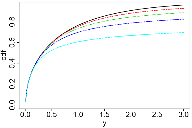
Figure 3b shows Wδ,δr(z)subscript𝑊subscript𝛿subscript𝛿𝑟𝑧W_{\delta_{\ell},\delta_{r}}(z) for δl=0subscript𝛿𝑙0\delta_{l}=0 and δr=1/10subscript𝛿𝑟110\delta_{r}=1/10. The transformation in Fig. 3a generates a right heavy tail version of U𝑈U (x-axis) by stretching only the positive axis (y-axis). By definition Wδ,δr(z)subscript𝑊subscript𝛿subscript𝛿𝑟𝑧W_{\delta_{\ell},\delta_{r}}(z) removes the heavier right tail in Z𝑍Z (positive y-axis). Figure 3c shows how Wδ(z)subscript𝑊𝛿𝑧W_{\delta}(z) operates for various degrees of heavy tails and z[0,3]𝑧03z\in[0,3]. If δ𝛿\delta is close to zero, then also Wδ(z)zsubscript𝑊𝛿𝑧𝑧W_{\delta}(z)\approx z; for larger δ𝛿\delta, the inverse maps z𝑧z to (much) smaller u𝑢u.

Remark 2.7 (Generalized transformation).

Transformation (2) can be generalized to

Z=Uexp(δ2α(U2)α),α>0.formulae-sequence𝑍𝑈𝛿2𝛼superscriptsuperscript𝑈2𝛼𝛼0Z=U\exp\left(\frac{\delta}{2\alpha}\left(U^{2}\right)^{\alpha}\right),\quad\alpha>0. (11)

The inner term U2superscript𝑈2U^{2} guarantees bijectivity for all α>0𝛼0\alpha>0. The inverse is

Wδ,α(z):=sgn(z)(W(δz2αδ))12α.assignsubscript𝑊𝛿𝛼𝑧sgn𝑧superscript𝑊𝛿superscript𝑧2𝛼𝛿12𝛼W_{\delta,\alpha}(z):=\operatorname{sgn}(z)\left(W\left(\frac{\delta z^{2\alpha}}{\delta}\right)\right)^{\frac{1}{2\alpha}}. (12)

For comparison with Tukey’s hh I consider α=1𝛼1\alpha=1 only. For α=1/2𝛼12\alpha=1/2 transformation (11) is closely related to skewed Lambert W ×\times FXsubscript𝐹𝑋F_{X} distributions.

2.4 Distribution and Density

For ease of notation let

z=yμxσx,u=Wδ(z), and x=Wτ(y)=uσx+μx.formulae-sequence𝑧𝑦subscript𝜇𝑥subscript𝜎𝑥formulae-sequence𝑢subscript𝑊𝛿𝑧 and 𝑥subscript𝑊𝜏𝑦𝑢subscript𝜎𝑥subscript𝜇𝑥\displaystyle z=\frac{y-\mu_{x}}{\sigma_{x}},\quad u=W_{\delta}(z),\text{ and }x=W_{\tau}(y)=u\sigma_{x}+\mu_{x}. (13)
Theorem 2.8 (Distribution and Density of Y𝑌Y).

The cdf and pdf of a location-scale heavy tail Lambert W ×\times FXsubscript𝐹𝑋F_{X} RV Y𝑌Y equal

GY(y𝜷,δ)=FX(Wδ(z)σx+μx𝜷)subscript𝐺𝑌conditional𝑦𝜷𝛿subscript𝐹𝑋subscript𝑊𝛿𝑧subscript𝜎𝑥conditionalsubscript𝜇𝑥𝜷\displaystyle G_{Y}\left(y\mid\boldsymbol{\beta},\delta\right)=F_{X}\left(W_{\delta}(z)\sigma_{x}+\mu_{x}\mid\boldsymbol{\beta}\right) (14)

and

gY(y𝜷,δ)subscript𝑔𝑌conditional𝑦𝜷𝛿\displaystyle g_{Y}\left(y\mid\boldsymbol{\beta},\delta\right) =fX(Wδ(yμxσx)σx+μx𝜷)Wδ(yμxσx)yμxσx[1+W(δ(yμxσx)2)].absentsubscript𝑓𝑋subscript𝑊𝛿𝑦subscript𝜇𝑥subscript𝜎𝑥subscript𝜎𝑥conditionalsubscript𝜇𝑥𝜷subscript𝑊𝛿𝑦subscript𝜇𝑥subscript𝜎𝑥𝑦subscript𝜇𝑥subscript𝜎𝑥delimited-[]1𝑊𝛿superscript𝑦subscript𝜇𝑥subscript𝜎𝑥2\displaystyle=f_{X}\left(W_{\delta}\left(\frac{y-\mu_{x}}{\sigma_{x}}\right)\sigma_{x}+\mu_{x}\mid\boldsymbol{\beta}\right)\cdot\frac{W_{\delta}\left(\frac{y-\mu_{x}}{\sigma_{x}}\right)}{\frac{y-\mu_{x}}{\sigma_{x}}\left[1+W\left(\delta\left(\frac{y-\mu_{x}}{\sigma_{x}}\right)^{2}\right)\right]}. (15)

Clearly, GY(y𝛃,δ=0)=FX(y𝛃)subscript𝐺𝑌conditional𝑦𝛃𝛿0subscript𝐹𝑋conditional𝑦𝛃G_{Y}\left(y\mid\boldsymbol{\beta},\delta=0\right)=F_{X}\left(y\mid\boldsymbol{\beta}\right) and gY(y𝛃,δ=0)=fX(y𝛃)subscript𝑔𝑌conditional𝑦𝛃𝛿0subscript𝑓𝑋conditional𝑦𝛃g_{Y}\left(y\mid\boldsymbol{\beta},\delta=0\right)=f_{X}\left(y\mid\boldsymbol{\beta}\right), since limδ0Wδ(z)=zsubscript𝛿0subscript𝑊𝛿𝑧𝑧\lim_{\delta\rightarrow 0}W_{\delta}(z)=z and limδ0W(δz2)=0subscript𝛿0𝑊𝛿superscript𝑧20\lim_{\delta\rightarrow 0}W(\delta z^{2})=0 for all z𝑧z\in\mathbb{R}.

For scale family or non-central, non-scale input set μx=0subscript𝜇𝑥0\mu_{x}=0 or μx=0,σx=1formulae-sequencesubscript𝜇𝑥0subscript𝜎𝑥1\mu_{x}=0,\sigma_{x}=1.

The explicit formula (15) allows a fast computation and theoretical analysis of the likelihood, which is essential for – either frequentist or Bayesian – statistical inference. Detailed properties of (15) are given in Section 4.1.

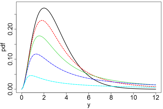
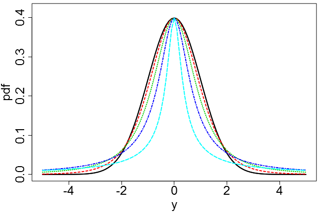
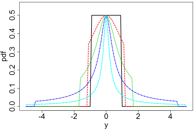
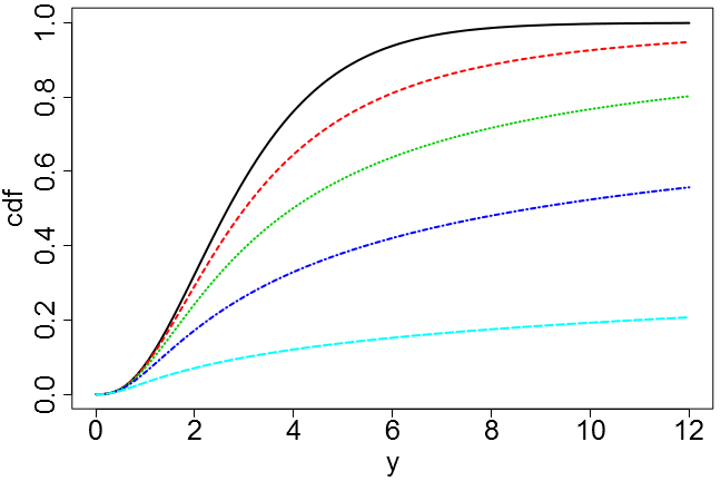
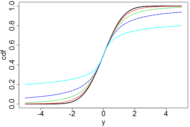
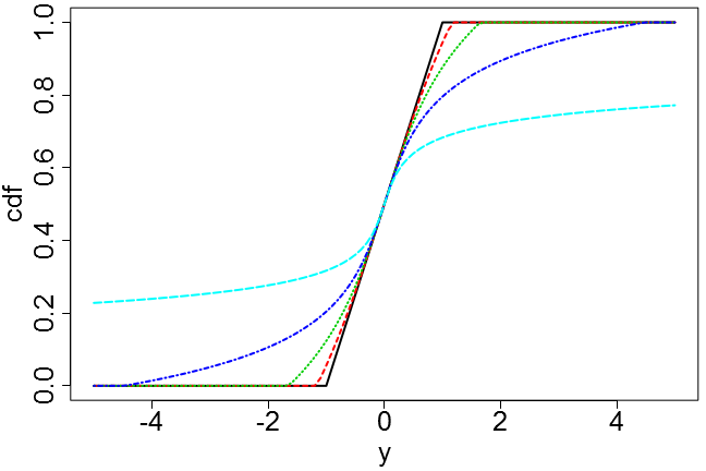
Figure 4 shows (14) and (15) for various δ0𝛿0\delta\geq 0 with for four different input XFX(x𝜷)similar-to𝑋subscript𝐹𝑋conditional𝑥𝜷X\sim F_{X}(x\mid\boldsymbol{\beta}): for δ=h=0𝛿0\delta=h=0 the input equals the output (solid black); for larger δ𝛿\delta the tails of GY(yθ)subscript𝐺𝑌conditional𝑦𝜃G_{Y}(y\mid\theta) and gY(yθ)subscript𝑔𝑌conditional𝑦𝜃g_{Y}(y\mid\theta) get heavier (dashed colored).

Refer to caption
(a)
Refer to caption
(b)
Refer to caption
(c)
Refer to caption
(d)
Refer to caption
(e)
Refer to caption
(a) Lambert W ×\times χk2superscriptsubscript𝜒𝑘2\chi_{k}^{2}
with 𝜷=k=1𝜷𝑘1\boldsymbol{\beta}=k=1.
Refer to caption
(b) Lambert W ×\times Γ(s,r)Γ𝑠𝑟\Gamma(s,r)
with 𝜷=(s,r)=(3,1)𝜷𝑠𝑟31\boldsymbol{\beta}=(s,r)=(3,1).
Refer to caption
(c) Lambert W ×\times 𝒩(μ,σ2)𝒩𝜇superscript𝜎2\mathcal{N}(\mu,\sigma^{2})
with 𝜷=(μ,σ)=(0,1)𝜷𝜇𝜎01\boldsymbol{\beta}=(\mu,\sigma)=(0,1).
Refer to caption
(d) Lambert W ×\times U(a,b)𝑈𝑎𝑏U(a,b)
with 𝜷=(a,b)=(1,1)𝜷𝑎𝑏11\boldsymbol{\beta}=(a,b)=(-1,1).
Figure 4: Pdf (top) and cdf (bottom) of a heavy-tail (a) “non-central, non-scaled”, (b) “scale”, and (c and d) “location-scale” Lambert W ×\times FXsubscript𝐹𝑋F_{X} RV Y𝑌Y for various degrees of heavy tails (color, dashed lines).
Corollary 2.9.

The cdf and pdf of Z𝑍Z in (3) equal

GZ(z𝜷,δ,δr)={GZ(z𝜷,δ),if z0,GZ(z𝜷,δr),if z>0,subscript𝐺𝑍conditional𝑧𝜷subscript𝛿subscript𝛿𝑟casessubscript𝐺𝑍conditional𝑧𝜷subscript𝛿if 𝑧0subscript𝐺𝑍conditional𝑧𝜷subscript𝛿𝑟if 𝑧0\displaystyle G_{Z}\left(z\mid\boldsymbol{\beta},\delta_{\ell},\delta_{r}\right)=\begin{cases}G_{Z}\left(z\mid\boldsymbol{\beta},\delta_{\ell}\right),&\text{if }z\leq 0,\\ G_{Z}\left(z\mid\boldsymbol{\beta},\delta_{r}\right),&\text{if }z>0,\end{cases} (16)

and

gZ(z𝜷,δ)={gZ(z𝜷,δ),if z0,gZ(z𝜷,δr),if z>0.subscript𝑔𝑍conditional𝑧𝜷𝛿casessubscript𝑔𝑍conditional𝑧𝜷subscript𝛿if 𝑧0subscript𝑔𝑍conditional𝑧𝜷subscript𝛿𝑟if 𝑧0\displaystyle g_{Z}\left(z\mid\boldsymbol{\beta},\delta\right)=\begin{cases}g_{Z}\left(z\mid\boldsymbol{\beta},\delta_{\ell}\right),&\text{if }z\leq 0,\\ g_{Z}\left(z\mid\boldsymbol{\beta},\delta_{r}\right),&\text{if }z>0.\end{cases} (17)

2.5 Quantile Function

Quantile fitting has been the standard technique to estimate μxsubscript𝜇𝑥\mu_{x}, σxsubscript𝜎𝑥\sigma_{x}, and δ𝛿\delta of Tukey’s hh. In particular, the median of Y𝑌Y and X𝑋X are equal. Thus for symmetric, location-scale family input the sample median of 𝐲𝐲\mathbf{y} is a robust estimate for μxsubscript𝜇𝑥\mu_{x} for any δ0𝛿0\delta\geq 0 (see also Section 5). General quantiles can be computed via (Hoaglin, 2006)

yα=uαexp(δ2uα2)σx+μx,subscript𝑦𝛼subscript𝑢𝛼𝛿2superscriptsubscript𝑢𝛼2subscript𝜎𝑥subscript𝜇𝑥y_{\alpha}=u_{\alpha}\exp\left(\frac{\delta}{2}u_{\alpha}^{2}\right)\sigma_{x}+\mu_{x}, (18)

where uα=Wδ(zα)subscript𝑢𝛼subscript𝑊𝛿subscript𝑧𝛼u_{\alpha}=W_{\delta}(z_{\alpha}) are the α𝛼\alpha-quantiles of FU(u)subscript𝐹𝑈𝑢F_{U}(u). As quantiles of U𝑈U are typically tabulated, or easily available in software packages, (18) can be computed very efficiently using uαsubscript𝑢𝛼u_{\alpha} and τ𝜏\tau.

This simple conversion can be especially useful for education: teaching heavy-tailed statistics in introductory courses soon becomes too difficult using e.g., Cauchy or α𝛼\alpha-stable distributions. Yet, transforming data via Lambert’s W𝑊W, using previously learned methods for the Gaussian case, and then transforming the inference back to the “heavy-tailed world” – e.g., transforming quantiles using (18) – is straightforward. Thus the Lambert W ×\times FXsubscript𝐹𝑋F_{X} framework can promote heavy-tailed statistics in introductory courses.

3 Tukey’s h distribution: Gaussian input

For Gaussian input Lambert W ×\times FXsubscript𝐹𝑋F_{X} equals Tukey’s hh, which has been studied extensively. Dutta and Babbel (2002) show that

𝔼Zn={0,if n is odd and n<1δ,n!(1nδ)(n+1)22n/2(n/2)!,if n is even and n<1δ,,if n>1δ,𝔼superscript𝑍𝑛cases0if n is odd and 𝑛1𝛿𝑛superscript1𝑛𝛿𝑛12superscript2𝑛2𝑛2if n is even and 𝑛1𝛿not-existsif 𝑛1𝛿\mathbb{E}Z^{n}=\begin{cases}0,&\text{if }\text{n is odd and }n<\frac{1}{\delta},\\ \frac{n!(1-n\delta)^{\frac{-(n+1)}{2}}}{2^{n/2}(n/2)!},&\text{if }\text{n is even and }n<\frac{1}{\delta},\\ \nexists,&\text{if }n>\frac{1}{\delta},\end{cases} (19)

which in particular implies (Headrick et al., 2008)

𝔼Z𝔼𝑍\displaystyle\mathbb{E}Z =𝔼Z3=0, if δ<1 and 1/3, respectivelyformulae-sequenceabsent𝔼superscript𝑍30 if 𝛿1 and 13, respectively\displaystyle=\mathbb{E}Z^{3}=0,\text{ if }\delta<1\text{ and }1/3\text{, respectively} (20)
and 𝔼Z2and 𝔼superscript𝑍2\displaystyle\text{ and }\mathbb{E}Z^{2} =1(12δ)3/2, if δ<12,𝔼Z4=31(14δ)5/2, if δ<14.formulae-sequenceabsent1superscript12𝛿32formulae-sequence if 𝛿12formulae-sequence𝔼superscript𝑍431superscript14𝛿52 if 𝛿14\displaystyle=\frac{1}{(1-2\delta)^{3/2}},\text{ if }\delta<\frac{1}{2},\quad\mathbb{E}Z^{4}=3\frac{1}{(1-4\delta)^{5/2}},\text{ if }\delta<\frac{1}{4}. (21)

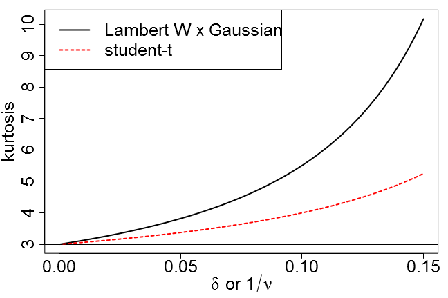
Thus the kurtosis of Y𝑌Y equals (see Fig. 5)

γ2(δ)=3(12δ)3(14δ)5/2 for δ<1/4.subscript𝛾2𝛿3superscript12𝛿3superscript14𝛿52 for 𝛿14\gamma_{2}(\delta)=3\frac{(1-2\delta)^{3}}{(1-4\delta)^{5/2}}\text{ for }\delta<1/4. (22)

For δ=0𝛿0\delta=0, (21) and (22) reduce to the familiar Gaussian values.

Corollary 3.1.

The cdf of Tukey’s hh equals

GY(yμx,σx,δ)=Φ(Wτ(y)μxσx),subscript𝐺𝑌conditional𝑦subscript𝜇𝑥subscript𝜎𝑥𝛿Φsubscript𝑊𝜏𝑦subscript𝜇𝑥subscript𝜎𝑥\displaystyle G_{Y}\left(y\mid\mu_{x},\sigma_{x},\delta\right)=\Phi\left(\frac{W_{\tau}(y)-\mu_{x}}{\sigma_{x}}\right), (23)

where Φ(u)Φ𝑢\Phi(u) is the cdf of a standard Normal. The pdf equals (for δ>0𝛿0\delta>0)

gY(yμx,σx,δ)subscript𝑔𝑌conditional𝑦subscript𝜇𝑥subscript𝜎𝑥𝛿\displaystyle g_{Y}\left(y\mid\mu_{x},\sigma_{x},\delta\right) =12πexp(1+δ2Wδ(yμxσx)2)11+W(δ(yμxσx)2)absent12𝜋1𝛿2subscript𝑊𝛿superscript𝑦subscript𝜇𝑥subscript𝜎𝑥211𝑊𝛿superscript𝑦subscript𝜇𝑥subscript𝜎𝑥2\displaystyle=\frac{1}{\sqrt{2\pi}}\exp{\left(-\frac{1+\delta}{2}W_{\delta}\left(\frac{y-\mu_{x}}{\sigma_{x}}\right)^{2}\right)}\cdot\frac{1}{1+W\left(\delta\left(\frac{y-\mu_{x}}{\sigma_{x}}\right)^{2}\right)} (24)
Proof.

Take X𝒩(μx,σx2)similar-to𝑋𝒩subscript𝜇𝑥superscriptsubscript𝜎𝑥2X\sim\mathcal{N}\left(\mu_{x},\sigma_{x}^{2}\right) in Theorem 2.8. ∎

Section 4.1 studies functional properties of (24) in more detail.

3.1 Tukey’s h versus student’s t

Student’s tνsubscript𝑡𝜈t_{\nu} distribution with ν𝜈\nu degrees of freedom is often used to model heavy-tailed data (Yan, 2005; Wong et al., 2009), as its tail index equals ν𝜈\nu. Thus the n𝑛nth moment of a student t RV T𝑇T exists if n<ν𝑛𝜈n<\nu. In particular,

𝔼T=𝔼T3=0 if ν<1 or<3,𝔼T2=νν2=112ν if 1ν<12,formulae-sequence𝔼𝑇𝔼superscript𝑇30 if 𝜈1 or3𝔼superscript𝑇2𝜈𝜈2112𝜈 if 1𝜈12\mathbb{E}T=\mathbb{E}T^{3}=0\text{ if }\nu<1\text{ or}<3,\quad\mathbb{E}T^{2}=\frac{\nu}{\nu-2}=\frac{1}{1-\frac{2}{\nu}}\text{ if }\frac{1}{\nu}<\frac{1}{2}, (25)

and kurtosis

γ2(ν)=3ν2ν4=3121ν141ν if 1ν<14.subscript𝛾2𝜈3𝜈2𝜈43121𝜈141𝜈 if 1𝜈14\gamma_{2}(\nu)=3\frac{\nu-2}{\nu-4}=3\frac{1-2\frac{1}{\nu}}{1-4\frac{1}{\nu}}\text{ if }\frac{1}{\nu}<\frac{1}{4}. (26)

Comparing (26) and (21) with (22) and (25) shows a natural association between 1/ν1𝜈1/\nu and δ𝛿\delta and a close similarity between the first four moments of student’s t𝑡t and Tukey’s hh (Fig. 5). By continuity and monotonicity, the first four moments of a location-scale t𝑡t distribution can always be exactly matched by a corresponding location-scale Lambert W ×\times Gaussian. Thus if student’s t𝑡t is used to model heavy tails, and not as the true distribution of a test statistic, it might be worthwhile to also fit heavy tail Lambert W ×\times Gaussian distributions for an equally valuable “second opinion”. For example, a parallel analysis on S&P 500 log\log-returns in Section 6.2 leads to divergent inference regarding the existence of fourth moments. Additionally, the Lambert W approach allows to Gaussianize and thus reveal hidden patterns in the data; patterns that can be easily overseen in presence of heavy tails (Section 6.3).
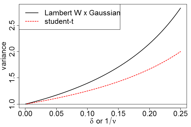
Refer to caption
(a) Variance
Refer to caption
(b) Kurtosis
Figure 5: Comparing moments of Lambert W ×\times Gaussian and student’s t𝑡t.

4 Parameter Estimation

For a sample of N𝑁N independent identically distributed (i.i.d.) observations 𝐲=(y1,,yN)𝐲subscript𝑦1subscript𝑦𝑁\mathbf{y}=(y_{1},\ldots,y_{N}) from transformation (6), θ=(𝜷,δ)𝜃𝜷𝛿\theta=(\boldsymbol{\beta},\delta) has to be estimated from the data. Due to the lack of a closed form pdf of Y𝑌Y, this has been typically done by matching quantiles or a method of moments estimator (Field, 2004; Morgenthaler and Tukey, 2000; Headrick et al., 2008). These inefficient methods can now be replaced by the – fast and usually efficient – maximum likelihood estimator (MLE) using the pdf in (15). Rayner and MacGillivray (2002) introduce a numerical MLE procedure based on quantile functions, but they conclude that “sample sizes significantly larger than 100100100 should be used to obtain reliable estimates through maximum likelihood”. Simulations in Section 5 show that log-likelihood maximization with the Lambert W methodology converges quickly and is accurate even for sample sizes as small as N=10𝑁10N=10.

4.1 Maximum Likelihood Estimation (MLE)

For an i.i.d. sample 𝐲gY(y𝜷,δ)similar-to𝐲subscript𝑔𝑌conditional𝑦𝜷𝛿\mathbf{y}\sim g_{Y}\left(y\mid\boldsymbol{\beta},\delta\right) the log-likelihood function equals

(θ𝐲)=i=1NloggY(yi𝜷,δ).conditional𝜃𝐲superscriptsubscript𝑖1𝑁subscript𝑔𝑌conditionalsubscript𝑦𝑖𝜷𝛿\ell\left(\theta\mid\mathbf{y}\right)=\sum_{i=1}^{N}\log g_{Y}(y_{i}\mid\boldsymbol{\beta},\delta). (27)

The MLE is that θ=(𝜷,δ)𝜃𝜷𝛿\theta=(\boldsymbol{\beta},\delta) which maximizes (27), i.e.

θ^MLE=(𝜷^,δ^)MLE=argmax𝜷,δ(𝜷,δ𝐲).subscript^𝜃𝑀𝐿𝐸subscript^𝜷^𝛿𝑀𝐿𝐸subscript𝜷𝛿𝜷conditional𝛿𝐲\widehat{\theta}_{MLE}=\left(\widehat{\boldsymbol{\beta}},\widehat{\delta}\right)_{MLE}=\arg\max_{\boldsymbol{\beta},\delta}\ell\left(\boldsymbol{\beta},\delta\mid\mathbf{y}\right). (28)

Since gY(yi𝜷,δ)subscript𝑔𝑌conditionalsubscript𝑦𝑖𝜷𝛿g_{Y}(y_{i}\mid\boldsymbol{\beta},\delta) is a function of fX(xi𝜷)subscript𝑓𝑋conditionalsubscript𝑥𝑖𝜷f_{X}(x_{i}\mid\boldsymbol{\beta}), the MLE depends on the specification of the input density. Eq. (27) can be decomposed as

(𝜷,δ𝐲)𝜷conditional𝛿𝐲\displaystyle\ell\left(\boldsymbol{\beta},\delta\mid\mathbf{y}\right) =(𝜷𝐱τ)+(τ𝐲),absentconditional𝜷subscript𝐱𝜏conditional𝜏𝐲\displaystyle=\ell\left(\boldsymbol{\beta}\mid\mathbf{x}_{\tau}\right)+\mathcal{R}\left(\tau\mid\mathbf{y}\right), (29)

where

(𝜷𝐱τ)=i=1NlogfX(Wδ(yiμxσx)σx+μx𝜷)=i=1NlogfX(𝐱τ𝜷)conditional𝜷subscript𝐱𝜏superscriptsubscript𝑖1𝑁subscript𝑓𝑋subscript𝑊𝛿subscript𝑦𝑖subscript𝜇𝑥subscript𝜎𝑥subscript𝜎𝑥conditionalsubscript𝜇𝑥𝜷superscriptsubscript𝑖1𝑁subscript𝑓𝑋conditionalsubscript𝐱𝜏𝜷\ell\left(\boldsymbol{\beta}\mid\mathbf{x}_{\tau}\right)=\sum_{i=1}^{N}\log f_{X}\left(W_{\delta}\left(\frac{y_{i}-\mu_{x}}{\sigma_{x}}\right)\sigma_{x}+\mu_{x}\mid\boldsymbol{\beta}\right)=\sum_{i=1}^{N}\log f_{X}\left(\mathbf{x}_{\tau}\mid\boldsymbol{\beta}\right) (30)

is the log-likelihood of the back-transformed data 𝐱τsubscript𝐱𝜏\mathbf{x}_{\tau} and

(τ𝐲)=i=1nlogR(μx,σx,δyi),conditional𝜏𝐲superscriptsubscript𝑖1𝑛𝑅subscript𝜇𝑥subscript𝜎𝑥conditional𝛿subscript𝑦𝑖\mathcal{R}\left(\tau\mid\mathbf{y}\right)=\sum_{i=1}^{n}\log R\left(\mu_{x},\sigma_{x},\delta\mid y_{i}\right), (31)

where

R(μx,σx,δyi)=Wδ(yiμxσx)yiμxσx[1+δ(Wδ(yiμxσx))2].𝑅subscript𝜇𝑥subscript𝜎𝑥conditional𝛿subscript𝑦𝑖subscript𝑊𝛿subscript𝑦𝑖subscript𝜇𝑥subscript𝜎𝑥subscript𝑦𝑖subscript𝜇𝑥subscript𝜎𝑥delimited-[]1𝛿superscriptsubscript𝑊𝛿subscript𝑦𝑖subscript𝜇𝑥subscript𝜎𝑥2R\left(\mu_{x},\sigma_{x},\delta\mid y_{i}\right)=\frac{W_{\delta}\left(\frac{y_{i}-\mu_{x}}{\sigma_{x}}\right)}{\frac{y_{i}-\mu_{x}}{\sigma_{x}}\left[1+\delta\left(W_{\delta}\left(\frac{y_{i}-\mu_{x}}{\sigma_{x}}\right)\right)^{2}\right]}. (32)

Note that R(μx,σx,δyi)𝑅subscript𝜇𝑥subscript𝜎𝑥conditional𝛿subscript𝑦𝑖R\left(\mu_{x},\sigma_{x},\delta\mid y_{i}\right) only depends on μx(𝜷)subscript𝜇𝑥𝜷\mu_{x}(\boldsymbol{\beta}) and σx(𝜷)subscript𝜎𝑥𝜷\sigma_{x}(\boldsymbol{\beta}) (and δ𝛿\delta), but not necessarily on every coordinate of 𝜷𝜷\boldsymbol{\beta}.

Refer to caption
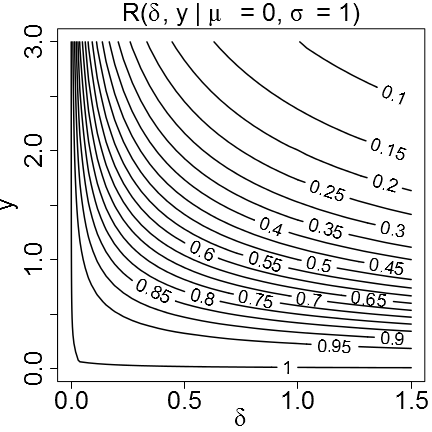
(a) Penalty R(μx,σx,δyi)𝑅subscript𝜇𝑥subscript𝜎𝑥conditional𝛿subscript𝑦𝑖R\left(\mu_{x},\sigma_{x},\delta\mid y_{i}\right) (32) as a function of δ𝛿\delta and y𝑦y (μx=0subscript𝜇𝑥0\mu_{x}=0 and σx=1subscript𝜎𝑥1\sigma_{x}=1).
Refer to caption
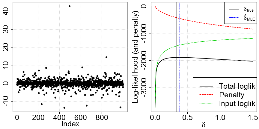
(b) Sample 𝐳𝐳\mathbf{z} of Lambert W ×\times Gaussian with δ=1/3𝛿13\delta=1/3 (left); Log-likelihood (θ𝐲)conditional𝜃𝐲\ell\left(\theta\mid\mathbf{y}\right) (solid, black) decomposes in input log-likelihood (dotted, green) and penalty (dashed, red).
Figure 6: Log-likelihood decomposition for Lambert W ×\times FXsubscript𝐹𝑋F_{X} distributions.

Decomposition (29) shows the difference between the exact MLE (𝜷^,δ^)^𝜷^𝛿\left(\widehat{\boldsymbol{\beta}},\widehat{\delta}\right) based on 𝐲𝐲\mathbf{y} and the approximate MLE 𝜷^𝐱τsubscript^𝜷subscript𝐱𝜏\widehat{\boldsymbol{\beta}}_{\mathbf{x}_{\tau}} based on 𝐱τsubscript𝐱𝜏\mathbf{x}_{\tau} alone: if we knew τ=(μx,σx,δ)𝜏subscript𝜇𝑥subscript𝜎𝑥𝛿\tau=(\mu_{x},\sigma_{x},\delta) beforehand, then we could back-transform 𝐲𝐲\mathbf{y} to 𝐱τsubscript𝐱𝜏\mathbf{x}_{\tau} and estimate 𝜷^𝐱τsubscript^𝜷subscript𝐱𝜏\widehat{\boldsymbol{\beta}}_{\mathbf{x}_{\tau}} from 𝐱τsubscript𝐱𝜏\mathbf{x}_{\tau} (maximize (30) with respect to 𝜷𝜷\boldsymbol{\beta}). In practice, however, τ𝜏\tau must also be estimated and this enters the likelihood via the additive term (τ𝐲)conditional𝜏𝐲\mathcal{R}\left(\tau\mid\mathbf{y}\right). A little calculation shows that for any yisubscript𝑦𝑖y_{i}\in\mathbb{R}, logR(μx,σx,δyi)0𝑅subscript𝜇𝑥subscript𝜎𝑥conditional𝛿subscript𝑦𝑖0\log R\left(\mu_{x},\sigma_{x},\delta\mid y_{i}\right)\leq 0 if δ0𝛿0\delta\geq 0, with equality if and only if δ=0𝛿0\delta=0. Thus (τ𝐲)conditional𝜏𝐲\mathcal{R}\left(\tau\mid\mathbf{y}\right) can be interpreted as a penalty for transforming the data. Maximizing (29) faces a trade-off between transforming the data to follow fX(x𝜷)subscript𝑓𝑋conditional𝑥𝜷f_{X}(x\mid\boldsymbol{\beta}) (and thus increasing (𝜷𝐱τ^)conditional𝜷subscript𝐱^𝜏\ell\left(\boldsymbol{\beta}\mid\mathbf{x}_{\widehat{\tau}}\right)) versus the penalty of a more extreme transformation (and thus decreasing (τ𝐲)conditional𝜏𝐲\mathcal{R}\left(\tau\mid\mathbf{y}\right)) – see Fig. 6b.

Figure 6a shows a contour plot of R(μx=0,σx=1,δy)𝑅formulae-sequencesubscript𝜇𝑥0subscript𝜎𝑥1conditional𝛿𝑦R\left(\mu_{x}=0,\sigma_{x}=1,\delta\mid y\right) as a function of δ𝛿\delta and y=z𝑦𝑧y=z. The penalty for transforming the data increases (in absolute value) either if δ𝛿\delta gets larger (for fixed y𝑦y) or for larger y𝑦y (for fixed δ𝛿\delta). In both cases, increasing δ𝛿\delta makes the transformed data Wδ(z)subscript𝑊𝛿𝑧W_{\delta}(z) get closer to 0=μx0subscript𝜇𝑥0=\mu_{x}, which in turn increases its input likelihood. For δ=0𝛿0\delta=0, the penalty disappears since input equals output; for y=0𝑦0y=0 there is no penalty since Wδ(0)=0subscript𝑊𝛿00W_{\delta}(0)=0 for all δ𝛿\delta.

Figure 6b shows a random sample (N=1000𝑁1000N=1000) 𝐳similar-to𝐳absent\mathbf{z}\sim Lambert W ×\times Gaussian with δ=1/3𝛿13\delta=1/3 and the decomposition of the log-likelihood as in (29). Since 𝜷=(0,1)𝜷01\boldsymbol{\beta}=(0,1) is known, the likelihood and penalty are only functions of δ𝛿\delta. The monotonicity of the penalty (decreasing, red) and the input likelihood (increasing, green) as a function of δ𝛿\delta is not particular to this sample, but holds true in general (see Theorem 4.1 below). This monotonicity in each component implies that their sum (black line) has a unique maximum; here δ^MLE=0.37subscript^𝛿𝑀𝐿𝐸0.37\widehat{\delta}_{MLE}=0.37 (blue, dashed vertical line).

The maximization of (29) can be carried out numerically. Here I show existence and uniqueness of δ^MLEsubscript^𝛿𝑀𝐿𝐸\widehat{\delta}_{MLE} assuming that μxsubscript𝜇𝑥\mu_{x} and σxsubscript𝜎𝑥\sigma_{x} are known. Theoretical results for θ^MLEsubscript^𝜃𝑀𝐿𝐸\widehat{\theta}_{MLE} remain for future work. Given the “nice” form of gY(y)subscript𝑔𝑌𝑦g_{Y}(y) - continuous, twice differentiable,555Assuming that fX()subscript𝑓𝑋f_{X}(\cdot) is twice differentiable. its support does not depend on the parameter, etc. - the MLE for θ=(𝜷,δ)𝜃𝜷𝛿\theta=(\boldsymbol{\beta},\delta) should have the usual optimality properties (Lehmann and Casella, 1998).

4.1.1 Properties of The MLE For The Heavy Tail Parameter

Without loss of generality let μx=0subscript𝜇𝑥0\mu_{x}=0 and σx=1subscript𝜎𝑥1\sigma_{x}=1. In this case

(δ𝐳)conditional𝛿𝐳\displaystyle\ell\left(\delta\mid\mathbf{z}\right) 12i=1N[Wδ(zi)]2+i=1NlogWδ(zi)zilog(1+δ[Wδ(zi)]2)proportional-toabsent12superscriptsubscript𝑖1𝑁superscriptdelimited-[]subscript𝑊𝛿subscript𝑧𝑖2superscriptsubscript𝑖1𝑁subscript𝑊𝛿subscript𝑧𝑖subscript𝑧𝑖1𝛿superscriptdelimited-[]subscript𝑊𝛿subscript𝑧𝑖2\displaystyle\propto-\frac{1}{2}\sum_{i=1}^{N}\left[W_{\delta}(z_{i})\right]^{2}+\sum_{i=1}^{N}\log\frac{W_{\delta}\left(z_{i}\right)}{z_{i}}-\log\left(1+\delta\left[W_{\delta}(z_{i})\right]^{2}\right) (33)
=1+δ2i=1N[Wδ(zi)]2i=1Nlog(1+δ[Wδ(zi)]2).absent1𝛿2superscriptsubscript𝑖1𝑁superscriptdelimited-[]subscript𝑊𝛿subscript𝑧𝑖2superscriptsubscript𝑖1𝑁1𝛿superscriptdelimited-[]subscript𝑊𝛿subscript𝑧𝑖2\displaystyle=-\frac{1+\delta}{2}\sum_{i=1}^{N}\left[W_{\delta}(z_{i})\right]^{2}-\sum_{i=1}^{N}\log\left(1+\delta\left[W_{\delta}(z_{i})\right]^{2}\right). (34)
Theorem 4.1 (Unique MLE for δ𝛿\delta).

Let Z𝑍Z have a Lambert W ×\times Gaussian distribution, where μx=0subscript𝜇𝑥0\mu_{x}=0 and σx=1subscript𝜎𝑥1\sigma_{x}=1 are assumed to be known and fixed. Also consider only the case δ[0,)𝛿0\delta\in[0,\infty).666While for some samples 𝐳𝐳\mathbf{z} the MLE also exists for δ<0𝛿0\delta<0, it can not be guaranteed for all 𝐳𝐳\mathbf{z}. If δ<0𝛿0\delta<0 (and z0𝑧0z\neq 0), then Wδ(z)subscript𝑊𝛿𝑧W_{\delta}(z) is either not unique in \mathbb{R} (principal and non-principal branch) or may not even have a real-valued solution.

  1. a)

    If

    i=1nzi4i=1nzi23,superscriptsubscript𝑖1𝑛superscriptsubscript𝑧𝑖4superscriptsubscript𝑖1𝑛superscriptsubscript𝑧𝑖23\frac{\sum_{i=1}^{n}z_{i}^{4}}{\sum_{i=1}^{n}z_{i}^{2}}\leq 3, (35)

    then δ^MLE=0subscript^𝛿𝑀𝐿𝐸0\widehat{\delta}_{MLE}=0.

If (35) does not hold, then

  1. b)

    δ^MLE>0subscript^𝛿𝑀𝐿𝐸0\widehat{\delta}_{MLE}>0 exists and is a positive solution to

    i=1Nzi2W(δzi2)(12Wδ(zi)2(12+11+W(δzi2)))=0.superscriptsubscript𝑖1𝑁superscriptsubscript𝑧𝑖2superscript𝑊𝛿superscriptsubscript𝑧𝑖212subscript𝑊𝛿superscriptsubscript𝑧𝑖21211𝑊𝛿superscriptsubscript𝑧𝑖20\sum_{i=1}^{N}z_{i}^{2}W^{\prime}(\delta z_{i}^{2})\left(\frac{1}{2}W_{\delta}\left(z_{i}\right)^{2}-\left(\frac{1}{2}+\frac{1}{1+W\left(\delta z_{i}^{2}\right)}\right)\right)=0. (36)
  2. c)

    There is only one such δ𝛿\delta satisfying (36), i.e. δ^MLEsubscript^𝛿𝑀𝐿𝐸\widehat{\delta}_{MLE} is unique.

Condition (35) says that δ^MLE>0subscript^𝛿𝑀𝐿𝐸0\widehat{\delta}_{MLE}>0 only if the data is heavy-tailed enough. Points b) and c) guarantee that there is no ambiguity in the heavy tail estimate. This is an advantage over student’s t𝑡t distribution, for example, which has numerical problems and local maxima for unknown (and small) ν𝜈\nu (\leftrightarrow large δ𝛿\delta) (see also Fernandez and Steel, 1999; Liu and Rubin, 1995). On the contrary, δ^MLEsubscript^𝛿𝑀𝐿𝐸\widehat{\delta}_{MLE} is always a global maximum.

The log-likelihood and its gradient depend on δ𝛿\delta and 𝐳𝐳\mathbf{z} only via Wδ(𝐳)subscript𝑊𝛿𝐳W_{\delta}(\mathbf{z}). Given the heavy tails in 𝐳𝐳\mathbf{z} (for δ>0𝛿0\delta>0) one might expect convergence issues for larger δ𝛿\delta (e.g. expected log-likelihood, Fisher information). However, Wδ(Z)𝒩(0,1)similar-tosubscript𝑊𝛿𝑍𝒩01W_{\delta}(Z)\sim\mathcal{N}(0,1) for the true δ0𝛿0\delta\geq 0, and close to a standard Gaussian if δ^MLEδsubscript^𝛿𝑀𝐿𝐸𝛿\widehat{\delta}_{MLE}\approx\delta. Thus the performance of the MLE should not get worse for large δ𝛿\delta as long as the initial estimate is close enough to the truth. Simulations in Section 5 support this conjecture, even for θ^MLEsubscript^𝜃𝑀𝐿𝐸\widehat{\theta}_{MLE}.

4.2 Iterative Generalized Method of Moments (IGMM)

A disadvantage of the MLE is the mandatory a-priori specification of the input distribution. Especially for heavy-tailed data the eye is a bad judgement to choose a particular parametric fX(x𝜷)subscript𝑓𝑋conditional𝑥𝜷f_{X}(x\mid\boldsymbol{\beta}). It would be useful to directly estimate τ𝜏\tau, without the intermediate step of estimating θ𝜃\theta first (and thus no distributional assumption for the input is necessary).

Goerg (2011) presented an estimator for τ𝜏\tau based on iterative generalized methods of moments (IGMM). The idea of IGMM is to find a τ𝜏\tau such that the back-transformed data 𝐱τsubscript𝐱𝜏\mathbf{x}_{\tau} has desired properties, e.g., is symmetric or has kurtosis 333. An estimator for μxsubscript𝜇𝑥\mu_{x}, σxsubscript𝜎𝑥\sigma_{x}, and δ𝛿\delta can be constructed completely analogously to the skewed IGMM, with the advantage that the heavy tail transformation is bijective (the skewed transformation is not). Since the algorithm is entirely analogous to the skewed case, details are given in the Supplementary Material, Appendix C.

An advantage of IGMM is that it requires less specific knowledge about the input distribution. Usually, it is also faster than the MLE. Once τ^IGMMsubscript^𝜏𝐼𝐺𝑀𝑀\widehat{\tau}_{IGMM} has been obtained, the back-transformed 𝐱τ^IGMMsubscript𝐱subscript^𝜏IGMM\mathbf{x}_{\widehat{\tau}_{\textsc{IGMM}}} can be used to check if X𝑋X has characteristics of a known parametric distribution FX(x𝜷)subscript𝐹𝑋conditional𝑥𝜷F_{X}(x\mid\boldsymbol{\beta}). It must be noted though that testing for a particular distribution FXsubscript𝐹𝑋F_{X} are too optimistic as 𝐱τ^subscript𝐱^𝜏\mathbf{x}_{\widehat{\tau}} will have “nicer” properties regarding FXsubscript𝐹𝑋F_{X} than the true 𝐱𝐱\mathbf{x} would have. However, estimating the transformation requires only three parameters and for a large enough sample, losing three degrees of freedom should not matter for all practical purposes.

5 Simulations

This section explores finite sample properties of estimators for θ=(μx,σx,δ)𝜃subscript𝜇𝑥subscript𝜎𝑥𝛿\theta=(\mu_{x},\sigma_{x},\delta) and (μy,σy)subscript𝜇𝑦subscript𝜎𝑦(\mu_{y},\sigma_{y}) under Gaussian input X𝒩(μx,σx2)similar-to𝑋𝒩subscript𝜇𝑥superscriptsubscript𝜎𝑥2X\sim\mathcal{N}(\mu_{x},\sigma_{x}^{2}). In particular, it compares Gaussian MLE (estimation of μysubscript𝜇𝑦\mu_{y} and σysubscript𝜎𝑦\sigma_{y} only), IGMM and Lambert W ×\times Gaussian MLE, and - for a heavy tail competitor – the median.777For IGMM, optimization was restricted to δ[0,10]𝛿010\delta\in[0,10]. All results below are based on n=1,000𝑛1000n=1,000 replications.

5.1 Estimating δ𝛿\delta Only

Here I show finite sample properties of δ^MLEsubscript^𝛿𝑀𝐿𝐸\widehat{\delta}_{MLE} for U𝒩(0,1)similar-to𝑈𝒩01U\sim\mathcal{N}(0,1), where μx=0subscript𝜇𝑥0\mu_{x}=0 and σx=1subscript𝜎𝑥1\sigma_{x}=1 are known and fixed. Theorem 4.1 shows that δ^MLEsubscript^𝛿𝑀𝐿𝐸\widehat{\delta}_{MLE} is unique: either at the boundary δ=0𝛿0\delta=0 or at the globally optimal solution to (36). Results in Table 1 were obtained by numerical optimization restricted to δ0𝛿0\delta\geq 0 (logδabsent𝛿\Leftrightarrow\log\delta\in\mathbb{R}) using the nlm function in R.

Table 1: Finite sample properties of δ^MLEsubscript^𝛿𝑀𝐿𝐸\widehat{\delta}_{MLE}. For each N𝑁N, δ𝛿\delta was estimated n=1,000𝑛1000n=1,000 times from a random sample 𝐳similar-to𝐳absent\mathbf{z}\sim Tukey’s hh. The left column for each δ𝛿\delta shows bias, δ^¯MLEδsubscript¯^𝛿𝑀𝐿𝐸𝛿\overline{\widehat{\delta}}_{MLE}-\delta; each right column shows the root mean square error (RMSE) times N𝑁\sqrt{N}.

N δ=0𝛿0\delta=0 δ=1/10𝛿110\delta=1/10 δ=1/3𝛿13\delta=1/3 δ=1/2𝛿12\delta=1/2 10 0.0250.0250.025 0.1910.1910.191 0.0170.017-0.017 0.3940.3940.394 0.0420.042-0.042 0.9150.9150.915 0.0820.082-0.082 1.1671.1671.167 50 0.0130.0130.013 0.1870.1870.187 0.0100.010-0.010 0.4920.4920.492 0.0180.018-0.018 0.9310.9310.931 0.0160.016-0.016 1.1561.1561.156 100 0.0100.0100.010 0.2000.2000.200 0.0100.010-0.010 0.5130.5130.513 0.0090.009-0.009 0.9140.9140.914 0.0060.006-0.006 1.2251.2251.225 400 0.0050.0050.005 0.1860.1860.186 0.0030.003-0.003 0.5280.5280.528 0.0000.0000.000 0.9270.9270.927 0.0040.004-0.004 1.2111.2111.211 1000 0.0030.0030.003 0.1970.1970.197 0.0000.0000.000 0.5320.5320.532 0.0010.001-0.001 0.9280.9280.928 0.0010.001-0.001 1.2031.2031.203 2000 0.0030.0030.003 0.2170.2170.217 0.0010.001-0.001 0.5230.5230.523 0.0000.0000.000 0.9350.9350.935 0.0010.001-0.001 1.1301.1301.130 N δ=1𝛿1\delta=1 δ=2𝛿2\delta=2 δ=5𝛿5\delta=5 10 0.0540.054-0.054 1.9871.9871.987 0.1040.104-0.104 3.3843.3843.384 0.0500.050-0.050 7.6017.6017.601 50 0.0170.017-0.017 1.9481.9481.948 0.0090.009-0.009 3.5293.5293.529 0.0140.0140.014 7.9427.9427.942 100 0.0140.014-0.014 2.0242.0242.024 0.0010.001-0.001 3.2943.2943.294 0.0110.0110.011 7.7987.7987.798 400 0.0010.0010.001 1.9191.9191.919 0.0020.002-0.002 3.4333.4333.433 0.0010.0010.001 7.8557.8557.855 1000 0.0010.0010.001 1.9551.9551.955 0.0010.0010.001 3.5533.5533.553 0.0010.001-0.001 7.4097.4097.409 2000 0.0010.0010.001 1.8961.8961.896 0.0000.0000.000 3.5083.5083.508 0.0010.001-0.001 7.5787.5787.578

Table 1 shows that the MLE is unbiased for every δ𝛿\delta and settles down (about N=100𝑁100N=100) to an asymptotic variance, which is increasing with δ𝛿\delta. Assuming μxsubscript𝜇𝑥\mu_{x} and σxsubscript𝜎𝑥\sigma_{x} to be known is unrealistic and thus these finite sample properties are only an indication of the behavior of the joint MLE, θ^MLEsubscript^𝜃𝑀𝐿𝐸\widehat{\theta}_{MLE}. Nevertheless they are very remarkable for extremely heavy-tailed data (δ>1𝛿1\delta>1), where standard statistical methods typically break down. One explanation in this behavior lies in the particular form of the likelihood (33) and its gradient (36) (Theorem 4.1). Although both depend on 𝐳𝐳\mathbf{z}, they only do so through Wδ(𝐳)=𝐮𝒩(0,1)subscript𝑊𝛿𝐳𝐮similar-to𝒩01W_{\delta}\left(\mathbf{z}\right)=\mathbf{u}\sim\mathcal{N}(0,1). Hence as long as δ^MLEsubscript^𝛿𝑀𝐿𝐸\widehat{\delta}_{MLE} is sufficiently close to the true δ𝛿\delta, (33) and (36) are functions of almost Gaussian RVs and standard asymptotic results should still apply.

5.2 Estimating All Parameters Jointly

Here we consider the realistic scenario where μxsubscript𝜇𝑥\mu_{x} and σxsubscript𝜎𝑥\sigma_{x} are also unknown. We consider various sample sizes (N=50𝑁50N=50, 100100100, and 100010001000) and different degrees of heavy tails, δ{0,1/3,1,1.5}𝛿01311.5\delta\in\{0,1/3,1,1.5\}, each one representing a particularly interesting situation: i) Gaussian data (does additional - superfluous - estimation of δ𝛿\delta affect other estimates?), ii) fourth moments do not exist anymore, iii) non-existing mean, iv) extremely heavy-tailed data – can we get useful estimates at all?

Table 2: In each subtable: (first rows) average, (middle rows) proportion of estimates below truth, (bottom rows) empirical standard deviation times N𝑁\sqrt{N}.
δ=0𝛿0\delta=0 median Gaussian MLE IGMM Lambert W MLE NA
N μysubscript𝜇𝑦\mu_{y} σysubscript𝜎𝑦\sigma_{y} μxsubscript𝜇𝑥\mu_{x} σxsubscript𝜎𝑥\sigma_{x} δ𝛿\delta σysubscript𝜎𝑦\sigma_{y} μxsubscript𝜇𝑥\mu_{x} σxsubscript𝜎𝑥\sigma_{x} δ𝛿\delta σysubscript𝜎𝑦\sigma_{y} ratio
505050 0.000.000.00 0.000.000.00 0.980.980.98 0.000.000.00 0.970.970.97 0.020.020.02 0.990.990.99 0.000.000.00 0.960.960.96 0.020.020.02 0.980.980.98 00
100100100 0.000.000.00 0.000.000.00 0.990.990.99 0.000.000.00 0.980.980.98 0.010.010.01 1.001.001.00 0.000.000.00 0.970.970.97 0.010.010.01 0.990.990.99 00
100010001000 0.000.000.00 0.000.000.00 1.001.001.00 0.000.000.00 0.990.990.99 0.000.000.00 1.001.001.00 0.000.000.00 0.990.990.99 0.000.000.00 1.001.001.00 00
505050 0.500.500.50 0.500.500.50 0.570.570.57 0.510.510.51 0.600.600.60 0.660.660.66 0.540.540.54 0.510.510.51 0.650.650.65 0.660.660.66 0.560.560.56 00
100100100 0.500.500.50 0.510.510.51 0.560.560.56 0.510.510.51 0.620.620.62 0.620.620.62 0.530.530.53 0.520.520.52 0.650.650.65 0.620.620.62 0.560.560.56 00
100010001000 0.500.500.50 0.490.490.49 0.520.520.52 0.490.490.49 0.620.620.62 0.560.560.56 0.520.520.52 0.490.490.49 0.630.630.63 0.560.560.56 0.520.520.52 00
505050 1.241.241.24 1.011.011.01 0.720.720.72 1.011.011.01 0.760.760.76 0.210.210.21 0.730.730.73 1.021.021.02 0.780.780.78 0.260.260.26 0.720.720.72 00
100100100 1.251.251.25 1.021.021.02 0.700.700.70 1.021.021.02 0.760.760.76 0.230.230.23 0.700.700.70 1.031.031.03 0.780.780.78 0.260.260.26 0.700.700.70 00
100010001000 1.261.261.26 0.980.980.98 0.730.730.73 0.980.980.98 0.790.790.79 0.220.220.22 0.730.730.73 0.980.980.98 0.790.790.79 0.220.220.22 0.730.730.73 00
(a) Truly Gaussian data: δ=0𝛿0\delta=0
δ=1/3𝛿13\delta=1/3 median Gaussian MLE IGMM Lambert W MLE NA
N μysubscript𝜇𝑦\mu_{y} σysubscript𝜎𝑦\sigma_{y} μxsubscript𝜇𝑥\mu_{x} σxsubscript𝜎𝑥\sigma_{x} δ𝛿\delta σysubscript𝜎𝑦\sigma_{y} μxsubscript𝜇𝑥\mu_{x} σxsubscript𝜎𝑥\sigma_{x} δ𝛿\delta σysubscript𝜎𝑦\sigma_{y} ratio
505050 0.000.000.00 0.000.000.00 1.981.981.98 0.000.000.00 1.071.071.07 0.290.290.29 \infty 0.000.000.00 1.011.011.01 0.330.330.33 \infty 00
100100100 0.000.000.00 0.000.000.00 2.032.032.03 0.000.000.00 1.041.041.04 0.310.310.31 \infty 0.000.000.00 1.001.001.00 0.330.330.33 \infty 00
100010001000 0.000.000.00 0.000.000.00 2.182.182.18 0.000.000.00 1.001.001.00 0.330.330.33 2.342.342.34 0.000.000.00 1.001.001.00 0.330.330.33 2.342.342.34 00
505050 0.500.500.50 0.510.510.51 0.780.780.78 0.500.500.50 0.380.380.38 0.630.630.63 0.600.600.60 0.500.500.50 0.520.520.52 0.540.540.54 0.540.540.54 00
100100100 0.500.500.50 0.510.510.51 0.780.780.78 0.510.510.51 0.420.420.42 0.610.610.61 0.600.600.60 0.500.500.50 0.510.510.51 0.540.540.54 0.540.540.54 00
100010001000 0.480.480.48 0.510.510.51 0.770.770.77 0.510.510.51 0.470.470.47 0.560.560.56 0.550.550.55 0.510.510.51 0.500.500.50 0.530.530.53 0.520.520.52 00
505050 1.271.271.27 2.212.212.21 6.566.566.56 1.441.441.44 1.451.451.45 1.101.101.10 NA𝑁𝐴NA 1.231.231.23 1.351.351.35 1.141.141.14 NA𝑁𝐴NA 00
100100100 1.301.301.30 2.332.332.33 11.2811.2811.28 1.431.431.43 1.421.421.42 1.121.121.12 NA𝑁𝐴NA 1.191.191.19 1.341.341.34 1.091.091.09 NA𝑁𝐴NA 00
100010001000 1.231.231.23 2.252.252.25 16.7616.7616.76 1.391.391.39 1.451.451.45 1.201.201.20 15.9715.9715.97 1.171.171.17 1.331.331.33 1.081.081.08 12.3012.3012.30 00
(b) No fourth moments: δ=1/3𝛿13\delta=1/3
δ=1𝛿1\delta=1 median Gaussian MLE IGMM Lambert W MLE NA
N μysubscript𝜇𝑦\mu_{y} σysubscript𝜎𝑦\sigma_{y} μxsubscript𝜇𝑥\mu_{x} σxsubscript𝜎𝑥\sigma_{x} δ𝛿\delta σysubscript𝜎𝑦\sigma_{y} μxsubscript𝜇𝑥\mu_{x} σxsubscript𝜎𝑥\sigma_{x} δ𝛿\delta σysubscript𝜎𝑦\sigma_{y} ratio
50 0.000.000.00 0.100.10-0.10 24.624.624.6 0.010.01-0.01 1.181.181.18 0.900.900.90 \infty 0.000.000.00 1.011.011.01 0.990.990.99 \infty 00
100 0.000.000.00 0.740.740.74 72.472.472.4 0.000.000.00 1.091.091.09 0.950.950.95 \infty 0.000.000.00 1.011.011.01 0.990.990.99 \infty 00
1000 0.000.000.00 3.843.843.84 348.1348.1348.1 0.000.000.00 1.011.011.01 1.001.001.00 \infty 0.000.000.00 1.001.001.00 1.001.001.00 \infty 00
50 0.530.530.53 0.520.520.52 1.01.01.0 0.510.510.51 0.340.340.34 0.650.650.65 111 0.510.510.51 0.520.520.52 0.520.520.52 111 00
100 0.500.500.50 0.520.520.52 1.01.01.0 0.510.510.51 0.380.380.38 0.630.630.63 111 0.500.500.50 0.530.530.53 0.530.530.53 111 00
1000 0.490.490.49 0.520.520.52 1.01.01.0 0.510.510.51 0.480.480.48 0.530.530.53 111 0.490.490.49 0.510.510.51 0.510.510.51 111 00
50 1.271.271.27 65.8565.8565.85 424.3424.3424.3 2.102.102.10 2.502.502.50 2.322.322.32 NA𝑁𝐴NA 1.191.191.19 1.701.701.70 2.162.162.16 NA𝑁𝐴NA 00
100 1.301.301.30 410.75410.75410.75 4050.24050.24050.2 2.012.012.01 2.282.282.28 2.592.592.59 NA𝑁𝐴NA 1.171.171.17 1.741.741.74 2.252.252.25 NA𝑁𝐴NA 00
1000 1.261.261.26 3307.583307.583307.58 104052.7104052.7104052.7 1.931.931.93 2.212.212.21 2.812.812.81 NA𝑁𝐴NA 1.111.111.11 1.641.641.64 2.182.182.18 NA𝑁𝐴NA 00
(c) Non-existing mean: δ=1𝛿1\delta=1
δ=1.5𝛿1.5\delta=1.5 median Gaussian MLE IGMM Lambert W MLE NA
N μysubscript𝜇𝑦\mu_{y} σysubscript𝜎𝑦\sigma_{y} μxsubscript𝜇𝑥\mu_{x} σxsubscript𝜎𝑥\sigma_{x} δ𝛿\delta σysubscript𝜎𝑦\sigma_{y} μxsubscript𝜇𝑥\mu_{x} σxsubscript𝜎𝑥\sigma_{x} δ𝛿\delta σysubscript𝜎𝑦\sigma_{y} ratio
50 0.020.02-0.02 6.846.846.84 309309309 0.020.02-0.02 1.231.231.23 1.371.371.37 \infty 0.010.01-0.01 1.001.001.00 1.491.491.49 \infty 0.010.010.01
100 0.000.000.00 51.1651.16-51.16 308030803080 0.010.01-0.01 1.121.121.12 1.441.441.44 \infty 0.000.000.00 1.011.011.01 1.501.501.50 \infty 0.000.000.00
1000 0.000.000.00 176.13176.13176.13 142511425114251 0.000.000.00 1.011.011.01 1.491.491.49 \infty 0.000.000.00 1.001.001.00 1.501.501.50 \infty 0.000.000.00
50 0.530.530.53 0.480.480.48 111 0.510.510.51 0.340.340.34 0.640.640.64 111 0.530.530.53 0.530.530.53 0.540.540.54 111 0.010.010.01
100 0.510.510.51 0.530.530.53 111 0.540.540.54 0.370.370.37 0.610.610.61 111 0.520.520.52 0.510.510.51 0.510.510.51 111 0.000.000.00
1000 0.500.500.50 0.500.500.50 111 0.500.500.50 0.470.470.47 0.540.540.54 111 0.490.490.49 0.530.530.53 0.520.520.52 111 0.000.000.00
50 1.321.321.32 1347.711347.711347.71 926192619261 2.572.572.57 3.203.203.20 3.123.123.12 NA𝑁𝐴NA 1.151.151.15 1.861.861.86 2.762.762.76 NA𝑁𝐴NA 0.010.010.01
100 1.331.331.33 42156.2842156.2842156.28 418435418435418435 2.392.392.39 2.872.872.87 3.443.443.44 NA𝑁𝐴NA 1.121.121.12 1.781.781.78 2.842.842.84 NA𝑁𝐴NA 0.000.000.00
1000 1.261.261.26 124462.82124462.82124462.82 390362939036293903629 2.182.182.18 2.662.662.66 3.673.673.67 NA𝑁𝐴NA 1.111.111.11 1.801.801.80 2.852.852.85 NA𝑁𝐴NA 0.000.000.00
(d) Extreme heavy tails: δ=1.5𝛿1.5\delta=1.5

The convergence tolerance for IGMM was set to tol=1.22104𝑡𝑜𝑙1.22superscript104tol=1.22\cdot 10^{-4}. Table 5 summarizes the simulation. Each sub-table is organized as follows: columns represent parameter estimates; the three main rows are the average over n=1,000𝑛1000n=1,000 replications (top), the proportion of estimates below the true value (middle), and the empirical standard deviation around the empirical average times N𝑁\sqrt{N} – not around the truth (bottom).

The Gaussian MLE estimates σysubscript𝜎𝑦\sigma_{y} directly, while IGMM and the Lambert W ×\times Gaussian MLE estimates δ𝛿\delta and σxsubscript𝜎𝑥\sigma_{x}, which implicitly give σ^ysubscript^𝜎𝑦\widehat{\sigma}_{y} through σy(δ,σx)=σx1(12δ)3/2subscript𝜎𝑦𝛿subscript𝜎𝑥subscript𝜎𝑥1superscript12𝛿32\sigma_{y}(\delta,\sigma_{x})=\sigma_{x}\cdot\frac{1}{\sqrt{(1-2\delta)^{3/2}}} if δ<1/2𝛿12\delta<1/2 (see (21)). For a fair comparison each sub-table also includes a column for σ^y=σ^x1(12δ^)3/2subscript^𝜎𝑦subscript^𝜎𝑥1superscript12^𝛿32\widehat{\sigma}_{y}=\widehat{\sigma}_{x}\cdot\frac{1}{\sqrt{(1-2\widehat{\delta})^{3/2}}}. Some of these entries contain “\infty”, even for δ<1/2𝛿12\delta<1/2; this occurs if at least one δ^1/2^𝛿12\widehat{\delta}\geq 1/2.

For any δ<1𝛿1\delta<1, μx=μysubscript𝜇𝑥subscript𝜇𝑦\mu_{x}=\mu_{y}, thus they can be directly compared. For δ1𝛿1\delta\geq 1, the mean does not exist; each sub-table for these δ𝛿\delta interprets μysubscript𝜇𝑦\mu_{y} as the median.

Gaussian data: δ=0𝛿0\delta=0

This setting checks if imposing the Lambert W framework, even though its use is superfluous, causes a quality loss in the estimation of μy=μxsubscript𝜇𝑦subscript𝜇𝑥\mu_{y}=\mu_{x} or σy=σxsubscript𝜎𝑦subscript𝜎𝑥\sigma_{y}=\sigma_{x}. Furthermore, critical values for H0:δ=0:subscript𝐻0𝛿0H_{0}:\delta=0 (Gaussian tails) can be obtained. Table 2a shows that all estimators are unbiased and quickly tend to a large-sample variance. Additional estimation of δ𝛿\delta does not affect the efficiency of μ^xsubscript^𝜇𝑥\widehat{\mu}_{x} compared to estimating solely μ𝜇\mu (both for IGMM and Lambert W ×\times Gaussian MLE). Estimating σysubscript𝜎𝑦\sigma_{y} directly by Gaussian MLE does not give better results than the Lambert W ×\times Gaussian MLE: both are unbiased and have similar standard deviation.

No fourth moment: δ=1/3𝛿13\delta=1/3

Here σy(δ,σx=1)=2.28subscript𝜎𝑦𝛿subscript𝜎𝑥12.28\sigma_{y}(\delta,\sigma_{x}=1)=2.28, but fourth moments do not exist anymore. This results in an increasing empirical standard deviation of σ^ysubscript^𝜎𝑦\widehat{\sigma}_{y} as N𝑁N grows. In contrast, estimates for σxsubscript𝜎𝑥\sigma_{x} are not drifting off. In presence of these large heavy tails the median is much less variable than Gaussian MLE and IGMM. Yet, Lambert W ×\times Gaussian MLE for μxsubscript𝜇𝑥\mu_{x} even outperforms the median.

Non-existing mean: δ=1𝛿1\delta=1

Here the mean is non-finite. Thus both sample moments diverge, and their standard errors are also growing quickly. The median still provides a very good estimate for the location, but is again inferior to both Lambert W estimators, which are unbiased and seem to converge to an asymptotic variance at rate N𝑁\sqrt{N}.

Extreme heavy tails: δ=1.5𝛿1.5\delta=1.5

As in Section 5.1, IGMM and Lambert W MLE continue to be unbiased even though the data is extremely heavy-tailed. Moreover, Lambert W MLE also has the smallest empirical standard deviation overall. In particular, the Lambert W MLE for μxsubscript𝜇𝑥\mu_{x} has an approximately 20%percent2020\% lower standard deviation than the median.

The last column shows that for some N𝑁N about 1%percent11\% of the n=1,000𝑛1000n=1,000 simulations generated invalid likelihood values (NA and \infty). Here the search for the optimal δ𝛿\delta lead into regions with a numerical overflow in the evaluation of Wδ(z)subscript𝑊𝛿𝑧W_{\delta}(z). For a comparable summary, these few cases were omitted and new simulations added until a full n=1,000𝑛1000n=1,000 finite estimates were found. Since this only happened in 1%percent11\% of the cases and also such heavy-tailed data is rarely encountered in practice, this numerical issue is not a real limitation in statistical practice.

5.3 Discussion of the Simulations

This simulation study confirms well-known facts about the sample average, standard deviation, and median and compares them to finite sample properties of the two Lambert W estimators. The median is known to be robust, which shows here as its quality does not depend on the thickness of the tails.

IGMM is unbiased for τ𝜏\tau independent of the magnitude of δ𝛿\delta. As expected the Lambert W MLE for θ𝜃\theta has the best properties: it is unbiased for all δ𝛿\delta, and for δ=0𝛿0\delta=0 it performs as well as the classic sample mean and standard deviation. For small δ𝛿\delta it has the same empirical standard deviation as the Gaussian MLE, but a lower one than the median for large δ𝛿\delta.

Hence the only advantage of estimating μysubscript𝜇𝑦\mu_{y} and σysubscript𝜎𝑦\sigma_{y} by sample moments of 𝐲𝐲\mathbf{y} is speed; otherwise the Lambert W ×\times Gaussian MLE is at least as good as the Gaussian MLE and clearly outperforms it for heavy-tailed data.

6 Applications

Tukey’s hh distribution has already proven useful to model heavy-tailed data, but parametric inference was limited to quantile fitting or methods of moments estimation (Headrick et al., 2008; Fischer, 2010; Field, 2004). Theorem 2.8 allows us to estimate θ𝜃\theta by ML.

This section shows the usefulness of the presented methodology on simulated as well as real world data: i) Section 6.1 demonstrates Gaussianizing on the Cauchy sample from the Introduction; ii) Section 6.2 shows that heavy tail Lambert W ×\times Gaussian distributions provide an excellent fit to daily S&P 500 log-return series; and iii) Section 6.3 shows how removing heavy tails reveals hidden patterns in power-law type data.

6.1 Estimating Location of a Cauchy With The Sample Mean

It is well-known that the sample mean 𝐲¯¯𝐲\overline{\mathbf{y}} is a poor estimate of the location parameter of a Cauchy distribution, since the sampling distribution of 𝐲¯¯𝐲\overline{\mathbf{y}} is again a Cauchy; in particular, its variance does not go to 00 for n𝑛n\rightarrow\infty.

Heavy-tailed Lambert W ×\times Gaussian distributions have similar properties to a Cauchy for δ1𝛿1\delta\approx 1. The mean of X𝑋X equals the location of Y𝑌Y, due to symmetry around μxsubscript𝜇𝑥\mu_{x} (for all δ0𝛿0\delta\geq 0) and c𝑐c, respectively. Thus we can estimate τ𝜏\tau from the Cauchy sample 𝐲𝐲\mathbf{y}, transform 𝐲𝐲\mathbf{y} to 𝐱τ^subscript𝐱^𝜏\mathbf{x}_{\widehat{\tau}}, estimate μxsubscript𝜇𝑥\mu_{x} from 𝐱τ^=Wτ^(𝐲)subscript𝐱^𝜏subscript𝑊^𝜏𝐲\mathbf{x}_{\widehat{\tau}}=W_{\widehat{\tau}}(\mathbf{y}), and thus obtain an estimate of c𝑐c.

The data 𝐲𝒞(0,1)similar-to𝐲𝒞01\mathbf{y}\sim\mathcal{C}(0,1) in Fig. 2a has heavy tails with two extreme (positive) samples. A Cauchy ML fit gives c^=0.03(0.055)^𝑐0.030.055\widehat{c}=0.03(0.055) and s^=0.86(0.053)^𝑠0.860.053\widehat{s}=0.86(0.053) (standard errors in parenthesis). A Lambert W ×\times Gaussian MLE gives μ^x=0.03(0.055)subscript^𝜇𝑥0.030.055\widehat{\mu}_{x}=0.03(0.055), σ^x=1.05(0.072)subscript^𝜎𝑥1.050.072\widehat{\sigma}_{x}=1.05(0.072), and δ^=0.86(0.082)^𝛿0.860.082\widehat{\delta}=0.86(0.082). Thus both fits correctly fail to reject μx=c=0subscript𝜇𝑥𝑐0\mu_{x}=c=0. Table 3a shows summary statistics on both samples. Since the Cauchy distribution does not have a well-defined mean, 𝐲¯=2.304(2.101)¯𝐲2.3042.101\overline{\mathbf{y}}=2.304(2.101) is not meaningful. However, 𝐱τ^MLEsubscript𝐱subscript^𝜏𝑀𝐿𝐸\mathbf{x}_{\widehat{\tau}_{MLE}} is approximately Gaussian and we use the sample average to do inference: 𝐱¯τ^MLE=0.033(0.0472)subscript¯𝐱subscript^𝜏𝑀𝐿𝐸0.0330.0472\overline{\mathbf{x}}_{\widehat{\tau}_{MLE}}=0.033(0.0472) correctly fails to reject a zero location for 𝐲𝐲\mathbf{y}. The transformed 𝐱τ^MLEsubscript𝐱subscript^𝜏𝑀𝐿𝐸\mathbf{x}_{\widehat{\tau}_{MLE}} features additional Gaussian characteristics (symmetric, no excess kurtosis), and even the null hypothesis of Normality cannot be rejected (p-value 0.5absent0.5\geq 0.5).

Figure 2d shows the running sample average for the original sample and its Gaussianized version. For a fair comparison τ^MLE(n)superscriptsubscript^𝜏𝑀𝐿𝐸𝑛\widehat{\tau}_{MLE}^{(n)} was re-estimated cumulatively for each n=5,,500𝑛5500n=5,\ldots,500, and then used to compute (x1,,xn)subscript𝑥1subscript𝑥𝑛(x_{1},\ldots,x_{n}). Even for small n𝑛n the transformation works extremely well: the highly influential point around n50𝑛50n\approx 50 greatly affects 𝐲¯¯𝐲\overline{\mathbf{y}}, but has no relevant effect on 𝐱¯τ^MLE(n)subscript¯𝐱superscriptsubscript^𝜏𝑀𝐿𝐸𝑛\overline{\mathbf{x}}_{\widehat{\tau}_{MLE}^{(n)}}. Overall, the sample average of the Gaussianized data has the usual good properties. And even for very small n𝑛n it is already clear that the location of the underlying Cauchy distribution is approximately zero.

Although a toy example, it shows that removing (strong) heavy tails from data works and provides new, “nice” data which can then be used for more refined methods.

Table 3: Summary statistics for observed (heavy-tailed) 𝐲𝐲\mathbf{y} and back-transformed (Gaussianized) data 𝐱τ^MLEsubscript𝐱subscript^𝜏𝑀𝐿𝐸\mathbf{x}_{\widehat{\tau}_{MLE}}. ** stands for <1016absentsuperscript1016<10^{-16}; * for <2.21016absent2.2superscript1016<2.2\cdot 10^{-16}.

Min Max Mean Median Stdev Skewness Kurtosis SW AD

()

𝐲𝐲\mathbf{y} 𝐱τ^subscript𝐱^𝜏\mathbf{x}_{\widehat{\tau}} 𝐱λ^subscript𝐱^𝜆\mathbf{x}_{\widehat{\lambda}} -161.59 -3.16 0 952.95 3.81 33.18 2.30 0.03 14.98 0.04 0.04 14.96 46.980 1.06 1.20 17.43 0.12 3.90 343.34 3.21 161.75 * 0.71 ** ** 0.51 **

(a) 𝐲𝒞(0,1)similar-to𝐲𝒞01\mathbf{y}\sim\mathcal{C}(0,1)
(Section 6.1)

𝐲𝐲\mathbf{y} 𝐱τ^subscript𝐱^𝜏\mathbf{x}_{\widehat{\tau}} -7.11 -2.42 4.99 2.23 0.05 0.05 0.04 0.04 0.95 0.71 -0.30 -0.04 7.70 2.93 * 0.24 * 0.18

(b) 𝐲𝐲\mathbf{y} = S&P 500
(Section 6.2)

𝐲𝐲\mathbf{y} 𝐱τ^subscript𝐱^𝜏\mathbf{x}_{\widehat{\tau}} 20 20 231300 157 689.4 89.0 87 87 6520.6 27.0 22.2 0.1 582.1 1.9 ** ** ** **

(c) 𝐲𝐲\mathbf{y} = solar flares
(Section 6.3)

6.2 Heavy Tails in Finance: S&P 500 Case Study

A lot of financial data displays negative skewness and excess kurtosis. Since financial data is in general not i.i.d., it is often modeled with a (skew) student-t distribution underlying a (generalized) auto-regressive conditional heteroskedastic (GARCH) (Engle, 1982; Bollerslev, 1986) or a stochastic volatility (SV) model (Melino and Turnbull, 1990; Deo et al., 2006). Using the Lambert W approach we can build upon the knowledge and implications of Gaussianity (and avoid deriving properties of a GARCH or SV model with heavy-tailed innovations), and simply “Gaussianize” the reutns before fitting more complex – GARCH or SV – models.

Remark 6.1.

Time series models with Lambert W ×\times Gaussian white noise are far beyond the scope of this work, but can be a direction of future research. Here I only consider the unconditional distribution.

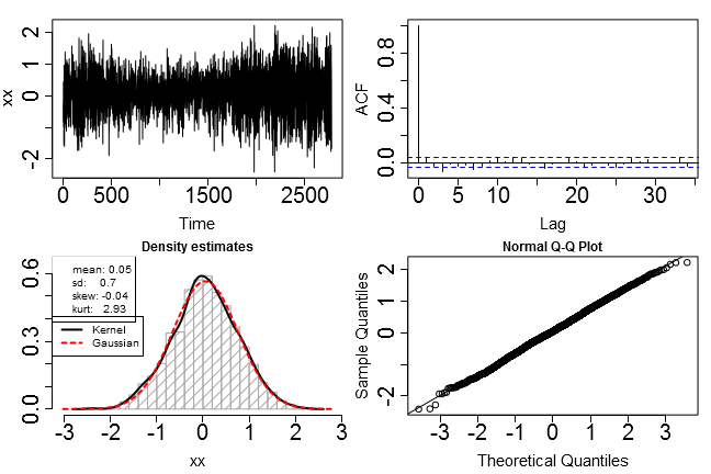
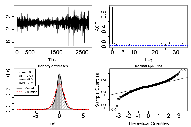
Figure 7a shows the S&P 500 log-returns with a total of N=2,780𝑁2780N=2,780 daily observations.888R package MASS, dataset SP500. Table 3b confirms the heavy tails (sample kurtosis 7.707.707.70), but also indicates negative skewness (0.2960.296-0.296). As the sample skewness γ^1(𝐲)subscript^𝛾1𝐲\widehat{\gamma}_{1}(\mathbf{y}) is very sensitive to outliers, we should test for symmetry by fitting a skewed distribution and testing its skewness parameter(s) for zero. In case of the double-tail Lambert W ×\times Gaussian this means to test H0:δ=δr=δ:subscript𝐻0subscript𝛿subscript𝛿𝑟𝛿H_{0}:\delta_{\ell}=\delta_{r}=\delta versus H1:δδr:subscript𝐻1subscript𝛿subscript𝛿𝑟H_{1}:\delta_{\ell}\neq\delta_{r}. Since the likelihood can now be computed by (29), we can use a likelihood ratio test with one degree of freedom (333 versus 444 parameters). The log-likelihood of the double-tail Lambert W ×\times Gaussian fit (Table 4a) equals 3606.0=2972.27+(633.73)3606.02972.27633.73-3606.0=-2972.27+(-633.73) (input + penalty), while the one δ𝛿\delta fit gives 3606.56=2971.47+(635.09)3606.562971.47635.09-3606.56=-2971.47+(-635.09). Here the double tails pay a lower penalty for transforming the data, but in turn give less Gaussian transformed sample. Comparing twice their difference to a χ12subscriptsuperscript𝜒21\chi^{2}_{1} distribution gives a p-value of 0.290.290.29. For comparison, a skew-t fit (Azzalini and Capitanio, 2003), with location c𝑐c, scale s𝑠s, shape α𝛼\alpha, and ν𝜈\nu degrees of freedom also yields 999Function st.mle in the R package sn. a non-significant α^^𝛼\widehat{\alpha} (Table 4b). Thus both fits cannot reject symmetry.
Refer to caption
(a) Observed heavy tail returns 𝐲𝐲\mathbf{y}
Refer to caption
(b) Gaussianized returns 𝐱τ^MLEsubscript𝐱subscript^𝜏𝑀𝐿𝐸\mathbf{x}_{\widehat{\tau}_{MLE}}
Figure 7: Lambert W Gaussianization of S&P 500 log-returns: τ^=(0.05,0.70,0.17)^𝜏0.050.700.17\widehat{\tau}=(0.05,0.70,0.17). In (a) and (b): data (top left); autocorrelation function (ACF) (top right); histogram, Gaussian fit, and KDE (bottom left); Normal QQ plot (bottom right).

Assume we have to make a decision if we should trade a certificate replicating the S&P 500. Since we can either buy or sell, it is not important if the average return is positive or negative, as long as it is significantly different from zero.

6.2.1 Gaussian Fit to Returns

If we ignore heavy tails and estimate (μy,σy)subscript𝜇𝑦subscript𝜎𝑦(\mu_{y},\sigma_{y}) by Gaussian MLE, μ^y=0subscript^𝜇𝑦0\widehat{\mu}_{y}=0 can not be rejected on a α=1%𝛼percent1\alpha=1\% level (Table 4e). However, a plain sample average over-estimates the variance in presence of heavy tails, and thus adds bias to the test statistic.

6.2.2 Heavy Tail Fit to Returns

Both a heavy tail Lambert W ×\times Gaussian (Table 4c) and student-t𝑡t fit (Table 4d) reject the zero mean null (p-values, 104superscript10410^{-4} and 31053superscript1053\cdot 10^{-5}, respectively). The standard errors for the location parameter are essentially the same.

While location and scale estimates are almost identical, the tail estimates lead to very different conclusions: while for ν^=3.71^𝜈3.71\widehat{\nu}=3.71 only moments up to order 333 exist, in the Lambert W ×\times Gaussian case moments up to order 555 exist (1/0.172=5.8110.1725.811/0.172=5.81). This is especially noteworthy as many theoretical results in the (financial) time series literature rely on finite fourth moments (Zadrozny, 2005; Mantegna and Stanley, 1998); consequently many empirical studies test if financial data actually satisfy this assumption (Cont, 2001; Huisman et al., 2001). For this particular dataset student’s t𝑡t and a Lambert W ×\times Gaussian fit give different answers to the same question. Since previous empirical studies often use student’s t𝑡t as a baseline (Wong et al., 2009), it might be worthwhile to re-examine their findings in light of heavy tail Lambert W ×\times Gaussian distributions.

Table 4: MLE fits to S&P 500 𝐲𝐲\mathbf{y} (a, b, c, d, e) and the Gaussianized data 𝐱τ^MLEsubscript𝐱subscript^𝜏𝑀𝐿𝐸\mathbf{x}_{\widehat{\tau}_{MLE}} (f).
Est. se t Pr(>tabsentdelimited-∣∣𝑡>\mid t\mid)
μxsubscript𝜇𝑥\mu_{x} 0.06 0.015 3.66 0.00
σxsubscript𝜎𝑥\sigma_{x} 0.71 0.016 44.00 0.00
δsubscript𝛿\delta_{\ell} 0.19 0.021 8.99 0.00
δrsubscript𝛿𝑟\delta_{r} 0.16 0.019 8.24 0.00
(a) double-tail Lambert W ×\times Gaussian = Tukey’s hhhh (S&P 500)
Est. se t Pr(>tabsentdelimited-∣∣𝑡>\mid t\mid)
c𝑐c 0.10 0.061 1.65 0.10
s𝑠s 0.67 0.017 38.47 0.00
α𝛼\alpha -0.08 0.101 -0.77 0.44
ν𝜈\nu 3.73 0.297 12.57 0.00
(b) skew t𝑡t (S&P 500)
Est. se t Pr(>tabsentdelimited-∣∣𝑡>\mid t\mid)
μxsubscript𝜇𝑥\mu_{x} 0.06 0.015 3.65 0.000
σxsubscript𝜎𝑥\sigma_{x} 0.71 0.016 43.95 0.000
δ𝛿\delta 0.17 0.016 11.05 0.000
(c) Lambert W ×\times Gaussian = Tukey’s hh (S&P 500)
Est. se t Pr(>tabsentdelimited-∣∣𝑡>\mid t\mid)
c𝑐c 0.06 0.015 3.65 0.00
s𝑠s 0.67 0.017 39.51 0.00
ν𝜈\nu 3.72 0.295 12.61 0.00
(d) student-t (S&P 500)
Est. se t Pr(>tabsentdelimited-∣∣𝑡>\mid t\mid)
μysubscript𝜇𝑦\mu_{y} 0.05 0.018 2.55 0.01
σysubscript𝜎𝑦\sigma_{y} 0.95 0.013 74.57 0.00
(e) Gaussian (S&P 500)
Est. se t Pr(>tabsentdelimited-∣∣𝑡>\mid t\mid)
μxτ^subscript𝜇subscript𝑥^𝜏\mu_{x_{\widehat{\tau}}} 0.05 0.013 3.81 0.00
σxτ^subscript𝜎subscript𝑥^𝜏\sigma_{x_{\widehat{\tau}}} 0.71 0.009 74.57 0.00
(f) Gaussian (𝐱τ^MLEsubscript𝐱subscript^𝜏𝑀𝐿𝐸\mathbf{x}_{\widehat{\tau}_{MLE}})

6.2.3 “Gaussianizing” Returns

A typical parameter inference study would conclude here. Using Lambert’s W function we can analyze the back-transformed 𝐱τ^MLEsubscript𝐱subscript^𝜏𝑀𝐿𝐸\mathbf{x}_{\widehat{\tau}_{MLE}} to test if a Lambert W ×\times Gaussian distribution is indeed appropriate. Figure 7b shows that 𝐱τ^MLEsubscript𝐱subscript^𝜏𝑀𝐿𝐸\mathbf{x}_{\widehat{\tau}_{MLE}} is indistinguishable from a Gaussian sample. Not even one Normality test can reject Gaussianity: p-values are 0.180.180.18, 0.180.180.18, 0.310.310.31, and 0.240.240.24, respectively (Anderson Darling, Cramer-von-Mises, Shapiro-Francia, Shapiro-Wilk; see Thode (2002)). Table 3b also shows that Lambert W “Gaussianiziation” was successful: γ^2(𝐱τ^)=2.93subscript^𝛾2subscript𝐱^𝜏2.93\widehat{\gamma}_{2}(\mathbf{x}_{\widehat{\tau}})=2.93 and γ^2(𝐱τ^)=0.039subscript^𝛾2subscript𝐱^𝜏0.039\widehat{\gamma}_{2}(\mathbf{x}_{\widehat{\tau}})=-0.039 are within the typical variation for a Gaussian sample. Thus

Y=(Ue0.1722U2)0.705+0.055,U=X0.0550.705,U𝒩(0,1)formulae-sequence𝑌𝑈superscript𝑒0.1722superscript𝑈20.7050.055formulae-sequence𝑈𝑋0.0550.705similar-to𝑈𝒩01\displaystyle Y=\left(Ue^{\frac{0.172}{2}U^{2}}\right)0.705+0.055,\quad U=\frac{X-0.055}{0.705},\quad U\sim\mathcal{N}(0,1) (37)

is an adequate (unconditional) Lambert W ×\times Gaussian model for the S&P 500 log-returns 𝐲𝐲\mathbf{y}. For trading, this means that the expected return is significantly larger than zero (μ^x=0.055>0subscript^𝜇𝑥0.0550\widehat{\mu}_{x}=0.055>0), and thus replicating certificates should be bought.

6.2.4 Gaussian MLE for Gaussianized Data

For δl=δrδ<1subscript𝛿𝑙subscript𝛿𝑟𝛿1\delta_{l}=\delta_{r}\equiv\delta<1, also μxμysubscript𝜇𝑥subscript𝜇𝑦\mu_{x}\equiv\mu_{y}. We can therefore replace testing μy=0subscript𝜇𝑦0\mu_{y}=0 versus μy0subscript𝜇𝑦0\mu_{y}\neq 0 for a non-Gaussian 𝐲𝐲\mathbf{y}, with the very well understood hypothesis test μx=0subscript𝜇𝑥0\mu_{x}=0 versus μx0subscript𝜇𝑥0\mu_{x}\neq 0 for the Gaussian 𝐱τ^MLEsubscript𝐱subscript^𝜏𝑀𝐿𝐸\mathbf{x}_{\widehat{\tau}_{MLE}}. In particular, standard errors based on σ^N^𝜎𝑁\frac{\widehat{\sigma}}{\sqrt{N}} - and thus t and p-values - should be closer to the “truth” (Table 4c and 4d) than a Gaussian MLE on the non-Gaussian 𝐲𝐲\mathbf{y} (Table 4e). Table 4f shows that standard errors for μ^𝐱subscript^𝜇𝐱\widehat{\mu}_{\mathbf{x}} are even a bit too small compared to the heavy-tailed versions. Since the “Gaussianizing” transformation was estimated, treating 𝐱τ^MLEsubscript𝐱subscript^𝜏𝑀𝐿𝐸\mathbf{x}_{\widehat{\tau}_{MLE}} as if it was original data is too optimistic regarding its Gaussianity (recall the penalty (31) in the total likelihood (29)).

This example confirms that if a model and its theoretical properties are based on Gaussianity, but the observed data is heavy-tailed, then Gaussianizing the data first gives more reliable inference than applying the Gaussian methods to the original, heavy-tailed data (Fig. 1). Clearly, a joint estimation of the model parameters based on Lambert W ×\times Gaussian errors (or any other heavy-tailed distribution) would be optimal. However, theoretical properties and estimation techniques may not have been developed and implemented yet, or are simply not known to researchers who are non-experts in heavy-tailed statistics. The Lambert Way to Gaussianize data thus is a pragmatic method to improve statistical inference on heavy-tailed data, while preserving the ease of usage and interpretation of Gaussian models.

6.3 Removing Power Law From Solar Flare Counts

The previous section focused on Lambert W ×\times FXsubscript𝐹𝑋F_{X} distributions as a “true” model for the data 𝐲𝐲\mathbf{y}. Here I consider it merely as a data transformation to remove heavy tails. In the same way as scaling 𝐲𝐲\mathbf{y} to zero-mean, unit-variance data, (𝐲𝐲¯)/σ^y𝐲¯𝐲subscript^𝜎𝑦(\mathbf{y}-\overline{\mathbf{y}})/\widehat{\sigma}_{y}, does not necessarily mean we believe the underlying process is Gaussian, we can also convert 𝐲𝐲\mathbf{y} to 𝐱τ=Wτ(𝐲)subscript𝐱𝜏subscript𝑊𝜏𝐲\mathbf{x}_{\tau}=W_{\tau}(\mathbf{y}) without assuming that 𝐲𝐲\mathbf{y} is actually Lambert W ×\times Gaussian. While 𝐱τ^subscript𝐱^𝜏\mathbf{x}_{\widehat{\tau}} might lose the interpretability of the observed data (e.g.  units become distorted), it can be helpful for exploratory data analysis (EDA), as the eye is a bad judgment to detect regularities corrupted by heavy tails. Removing them can reveal hidden patterns and thus greatly improve the accuracy of statistical inference for 𝐲𝐲\mathbf{y}.

Refer to caption
(a) Peak X-ray intensity 𝐲𝐲\mathbf{y}.
Refer to caption
(b) KDE fit of 𝐲𝐲\mathbf{y} over time. For better visualization y<165𝑦165y<165.
Refer to caption
(c) KDE fit of 𝐱τ^subscript𝐱^𝜏\mathbf{x}_{\widehat{\tau}} over time (no truncation in x𝑥x).
Refer to caption
(d) Zoom to 𝐲400𝐲400\mathbf{y}\leq 400; horizontal lines y^min=323±89subscript^𝑦plus-or-minus32389\widehat{y}_{\min}=323\pm 89 for power-law cut-off.
Refer to caption
(e) Back-transformed 𝐱τ^1subscript𝐱subscript^𝜏1\mathbf{x}_{\widehat{\tau}_{1}}, τ^1=(74.46,26.32,1.53)subscript^𝜏174.4626.321.53\widehat{\tau}_{1}=(74.46,26.32,1.53); horizontal lines at Wτ^1(y^min±89)=114.94subscript𝑊subscript^𝜏1plus-or-minussubscript^𝑦89114.94W_{\widehat{\tau}_{1}}(\widehat{y}_{\min}\pm 89)=114.94 and (110.96,117.58)110.96117.58(110.96,117.58).
Refer to caption
(f) Back-transformed 𝐱τ^subscript𝐱^𝜏\mathbf{x}_{\widehat{\tau}}, τ^=(86.97,26.80,0,2.37)^𝜏86.9726.8002.37\widehat{\tau}=(86.97,26.80,0,2.37); horizontal lines at Wτ^(y^min±89)=121.16subscript𝑊^𝜏plus-or-minussubscript^𝑦89121.16W_{\widehat{\tau}}(\widehat{y}_{\min}\pm 89)=121.16 and (117.74,123.37)117.74123.37(117.74,123.37).
Figure 8: Peak X-ray count rates of solar flares.

Here I study solar flare gamma-ray count rates (Clauset et al., 2009; Newman, 2005). The data101010Dataset SolarFlares in the LambertW package. were collected approximately four times a day from Feb. 1980 until Nov. 1989 giving T=12,773𝑇12773T=12,773 observations. See Dennis et al. (1991) for details and scientific background.

The gamma-ray count rates exhibit a strong right heavy tail (Fig. 8a), which makes more detailed visual inspection as well as simple EDA difficult. A zoom to yi400subscript𝑦𝑖400y_{i}\leq 400 in Fig. 8d shows that a lot of counts lie between 505050 and 100100100 and this level drops off at the end of the observation cycle. This drop is not an intrinsic characteristic of solar flares but due to a decreasing sensitivity of the X-ray detectors over time (Dennis et al., 1991). For the sake of comparison with Clauset et al. (2009); Newman (2005) most estimates are based on all T=12,773𝑇12773T=12,773 observations. Figures 8d, 8e, and 8f also show separate density estimates for the first 4,00040004,000 and last 2,27322732,273 observations, and while the estimates change, the qualitative findings do not.

Clauset et al. (2009) find that a power-law (a^=1.79(0.02)^𝑎1.790.02\widehat{a}=1.79(0.02)) with cut-off (y^min=323(89)subscript^𝑦32389\widehat{y}_{\min}=323(89)) gives the best fit amongst various alternatives. However, this first EDA might not be complete: not only visually heavy tails can obscure underlying non-trivial structure, but also estimates - such as the power law fit or non-parametric density estimates (Fig. 8d and 8b) - are affected by the heavy right tail. Here I show that Gaussianizing this data reveals new insights for the data-generating process, with a new interpretation for the optimality of the cut-off.

A Lambert W ×\times Gaussian MLE fit θ^=(μ^x,σ^x,δ^,δr^)=(86.97,26.80,0,2.37)^𝜃subscript^𝜇𝑥subscript^𝜎𝑥^subscript𝛿^subscript𝛿𝑟86.9726.8002.37\widehat{\theta}=(\widehat{\mu}_{x},\widehat{\sigma}_{x},\widehat{\delta_{\ell}},\widehat{\delta_{r}})=(86.97,26.80,0,2.37) confirms that only the right tail (tail index 1/2.373=0.42112.3730.4211/2.373=0.421) needs a Gaussianizing transformation.111111For comparison Fig. 8e also shows the back-transformed data 𝐱τ^1subscript𝐱subscript^𝜏1\mathbf{x}_{\widehat{\tau}_{1}} using the same δ𝛿\delta on each tail (τ^1=(74.46,26.32,1.53)subscript^𝜏174.4626.321.53\widehat{\tau}_{1}=(74.46,26.32,1.53)). However, due to the clear right heavy tail I will continue with the (δl,δr)subscript𝛿𝑙subscript𝛿𝑟(\delta_{l},\delta_{r}) transformation.

The last column of Fig. 8 shows EDA for the Gaussianized data. Removing the heavy right tail reveals a bimodal structure, which gives additional meaning to y^min=323subscript^𝑦323\widehat{y}_{\min}=323. The Gaussianized cut-off value equals Wτ^(323)=121.16subscript𝑊^𝜏323121.16W_{\widehat{\tau}}(323)=121.16 with the transformed standard deviation interval [117.74,123.37]117.74123.37[117.74,123.37] (corresponding to 323±89plus-or-minus32389323\pm 89). Fitting a two component Gaussian mixture model to 𝐱τ^subscript𝐱^𝜏\mathbf{x}_{\widehat{\tau}} yields λ^𝒩1(67.10,14.042)+(1λ^)𝒩2(113.12,14.272)^𝜆subscript𝒩167.10superscript14.0421^𝜆subscript𝒩2113.12superscript14.272\widehat{\lambda}\,\mathcal{N}_{1}(67.10,14.04^{2})+(1-\widehat{\lambda})\,\mathcal{N}_{2}(113.12,14.27^{2}) with λ^=0.52^𝜆0.52\widehat{\lambda}=0.52 and optimal decision boundary between classes of 90.4890.4890.48. The mean of the larger component, 113.12113.12113.12, lies within one standard deviation of the optimal Gaussianized cut-off 121.16121.16121.16: for lower cut-offs the left-tail of the larger component – or for much lower cut-offs even the smaller component – would counteract the power-law decay of the upper gamma-ray count rates.

As mentioned above, this analysis is not intended to describe the underlying process of solar flare gamma rays; it should rather show new insights that can be gained by Gaussianizing. Future research based on these new findings might lead to new physical interpretations of the statistical properties gamma-ray count rates, see for example Aschwanden (2011).

7 Discussion and Outlook

I adapt the skewed Lambert W input / output framework to introduce heavy tails in continuous RVs XFX(x)similar-to𝑋subscript𝐹𝑋𝑥X\sim F_{X}(x). For Gaussian input this not only contributes to existing work on Tukey’s hh distribution, but also gives convincing empirical results: unimodal data with heavy tails can be transformed to Gaussian data/RVs. Properties of a Gaussian model 𝒩subscript𝒩\mathcal{M}_{\mathcal{N}} on the back-transformed data mimic the features of the “true” skewed, heavy-tailed model Gsubscript𝐺\mathcal{M}_{G} very closely.

Since Gaussianity is the single most typical, and often required, assumption in many areas of statistics, machine learning, and signal processing, future research can take many directions. From a theoretical perspective properties of Lambert W ×\times FXsubscript𝐹𝑋F_{X} distributions viewed as a generalization of already well-known distributions FXsubscript𝐹𝑋F_{X} can be studied. This area will profit from existing literature on the Lambert W function, which has been discovered only recently by the statistics community. Empirical work can focus on transforming the data and compare performances of approximate Gaussian versus joint heavy-tail analysis. The comparisons in this work showed that approximate inference for Gaussianized data is comparable with the direct heavy tail modeling, and so provides an easy tool to improve inference for heavy-tailed data in statistical practice.

I also provide the R package LambertW, publicly available at CRAN, to facilitate the use of Lambert W ×\times FXsubscript𝐹𝑋F_{X} distributions in practice.

Acknowledgments

I want to thank Andrew F. Siegel who brought Tukey’s hh distribution to my attention, and Brian R. Dennis who gave detailed background information and suggestions on the solar flares dataset.

References

  • Achim et al. (2003) Achim, A., P. Tsakalides, and A. Bezerianos (2003). SAR image denoising via Bayesian wavelet shrinkage based on heavy-tailed modeling. Geoscience and Remote Sensing, IEEE Transactions on 41(8), 1773 – 1784.
  • Aschwanden (2011) Aschwanden, M. J. (2011). The State of Self-Organized Criticality of the Sun During the Last Three Solar Cycles. II. Theoretical Model. Solar Physics 274, 119–129.
  • Aysal and Barner (2006) Aysal, T. C. and K. E. Barner (2006). Second-order heavy-tailed distributions and tail analysis. IEEE Transactions on Signal Processing 54(7), 2827–2832.
  • Azzalini and Capitanio (2003) Azzalini, A. and A. Capitanio (2003). Distributions generated by perturbation of symmetry with emphasis on a multivariate skew t distribution. Journal of the Royal Statistical Society ser B 65, 367–389.
  • Baek and Pipiras (2010) Baek, C. and V. Pipiras (2010). Estimation of parameters in heavy-tailed distribution when its second order tail parameter is known. Journal of Statistical Planning and Inference 140(7), 1957 – 1967.
  • Blaylock et al. (1980) Blaylock, J. R., L. E. Salathe, and R. D. Green (1980). A note on the Box-Cox transformation under heteroskedasticity. Western Journal of Agricultural Economics 05(02), 129–136.
  • Bollerslev (1986) Bollerslev, T. (1986). Generalized autoregressive conditional heteroskedasticity. Journal of Econometrics 31, 307 – 327.
  • Brockwell and Davis (1998) Brockwell, P. J. and R. A. Davis (1998). Time Series: Theory and Methods. Springer Series in Statistics.
  • Clauset et al. (2009) Clauset, A., C. R. Shalizi, and M. E. J. Newman (2009). Power-law distributions in empirical data. SIAM Review 51, 661–703.
  • Cont (2001) Cont, R. (2001). Empirical properties of asset returns: stylized facts and statistical issues. Quantitative Finance 1, 223–236.
  • Corless et al. (1996) Corless, R. M., G. H. Gonnet, D. E. G. Hare, and D. J. Jeffrey (1996). On the Lambert W function. Advances in Computational Mathematics 5, 329–359.
  • Dennis et al. (1991) Dennis, B. R., L. E. Orwig, G. S. Kennard, G. J. Labow, R. A. Schwartz, A. R. Shaver, and A. K. Tolbert (1991). The complete Hard X Ray Burst Spectrometer event list, 1980-1989. Available http://adsabs.harvard.edu/abs/1991chxb.book.....D and http://umbra.nascom.nasa.gov/smm/hxrbs.html.
  • Deo et al. (2006) Deo, R., C. Hurvich, and Y. Lu (2006). Forecasting Realized Volatility Using a Long Memory Stochastic VolatilityModel: Estimation, Prediction and Seasonal Adjustment. Journal of Econometrics 127, 29 – 58.
  • Dutta and Babbel (2002) Dutta, K. K. and D. Babbel (2002). On Measuring Skewness and Kurtosis in Short Rate Distributions: The Case of the US Dollar London Inter Bank Offer Rates. Technical report, Wharton School Center for Financial Institutions, University of Pennsylvania.
  • Engle (1982) Engle, R. (1982). Autoregressive conditional heteroskedasticity with estimates of the variance of U.K. inflation. Econometrica 50, 987 – 1008.
  • Fernandez and Steel (1999) Fernandez, C. and M. F. J. Steel (1999). Multivariate Student-t Regression Models: Pitfalls and Inference. Biometrika 86, 153–167.
  • Field and Genton (2006) Field, C. and M. G. Genton (2006). The Multivariate g-and-h Distribution. Technometrics 48(1), 104–111.
  • Field (2004) Field, C. A. (2004). Using the gh distribution to model extreme wind speeds. Journal of Statistical Planning and Inference 122(1-2), 15 – 22.
  • Fischer (2010) Fischer, M. (2010). Generalized Tukey-type distributions with application to financial and teletraffic data. Statistical Papers 51, 41–56. 10.1007/s00362-007-0114-z.
  • Galassi et al. (2011) Galassi, M., J. Davies, J. Theiler, B. Gough, G. Jungman, P. Alken, M. Booth, and F. Rossi (2011). GNU Scientific Library Reference Manual (3rd ed.). ISBN 0954612078; www.gnu.org/software/gsl.
  • Gidlund and Debernardi (2009) Gidlund, M. and N. Debernardi (2009). Scheduling performance of heavy-tailed data traffic in wireless high-speed shared channels. In Proceedings of the 2009 IEEE conference on Wireless Communications & Networking Conference, WCNC’09, Piscataway, NJ, USA, pp. 1818–1823. IEEE Press.
  • Goerg (2011) Goerg, G. M. (2011). Lambert W Random Variables - A New Family of Generalized Skewed Distributions with Applications to Risk Estimation. The Annals of Applied Statistics 5(3), p. 2197 – 2230. arxiv.org/abs/0912.4554.
  • Goncalves and Meddahi (2011) Goncalves, S. and N. Meddahi (2011). Box-Cox transforms for realized volatility. Journal of Econometrics 160(1), 129–144.
  • Granger and Joyeux (2001) Granger, C. W. J. and R. Joyeux (2001). An introduction to long-memory time series models and fractional differencing. Journal of Time Series Analysis 1, 15 – 30.
  • Headrick et al. (2008) Headrick, T. C., R. K. Kowalchuk, and Y. Sheng (2008). Parametric Probability Densities and Distribution Functions for Tukey g-and-h Transformations and their Use for Fitting Data. Applied Mathematical Sciences 2(9), 449 – 462.
  • Hoaglin (2006) Hoaglin, D. C. (2006). Summarizing Shape Numerically: The g-and-h Distributions, pp.  461–513. Hoboken, NJ, USA: John Wiley and Sons, Inc.
  • Huisman et al. (2001) Huisman, R., K. G. Koedijk, C. J. M. Kool, and F. Palm (2001). Tail-index estimates in small samples. Journal of Business & Economic Statistics 19(2), 208–16.
  • Hwang et al. (1994) Hwang, J., S. Lay, and A. Lippman (1994). Nonparametric multivariate density estimation: A comparative study. IEEE Trans. Signal Processing 42, 2795–2810.
  • Ilow (2000) Ilow, J. (2000). Forecasting network traffic using farima models with heavy tailed innovations. Acoustics, Speech, and Signal Processing, IEEE International Conference on 6, 3814–3817.
  • Jodrá (2009) Jodrá, P. (2009). A closed-form expression for the quantile function of the Gompertz-Makeham distribution. Math. Comput. Simul. 79, 3069–3075.
  • Kim and White (2003) Kim, T.-H. and H. White (2003). On More Robust Estimation of Skewness and Kurtosis: Simulation and Application to the S&P500 Index.
  • Lawrance (1987) Lawrance, A. J. (1987). A note on the variance of the Box-Cox regression transformation estimate. Journal of the Royal Statistical Society. Series C (Applied Statistics) 36(2), 221–223.
  • Lehmann and Casella (1998) Lehmann, E. L. and G. Casella (1998). Theory of Point Estimation (2 ed.). Springer Texts in Statistics.
  • Liu and Rubin (1995) Liu, C. and D. B. Rubin (1995). ML Estimation of the t distribution using EM and its extensions, ECM and ECME. Statistica Sinica 5, 19–39.
  • Liu et al. (2009) Liu, H., J. Lafferty, and L. Wasserman (2009). The Nonparanormal: Semiparametric Estimation of High Dimensional Undirected Graphs. Journal of Machine Learning Research 10, 2295–2328.
  • Maiboroda and Markovich (2004) Maiboroda, R. and N. Markovich (2004). Estimation of heavy-tailed probability density function with application to web data. Computational Statistics 19, 569–592. 10.1007/BF02753913.
  • Mantegna and Stanley (1998) Mantegna, R. N. and H. E. Stanley (1998). Modeling of financial data: Comparison of the truncated Lévy flight and the ARCH(1) and GARCH(1,1) processes. Physica A: Statistical and Theoretical Physics 254(1-2), 77 – 84.
  • Markovich (2005) Markovich, N. M. (2005). Accuracy of transformed kernel density estimates for a heavy-tailed distribution. Autom. Remote Control 66, 217–232.
  • Melino and Turnbull (1990) Melino, A. and S. M. Turnbull (1990). Pricing foreign currency options with stochastic volatility. Journal of Econometrics 45(1-2), 239 – 265.
  • Morgenthaler and Tukey (2000) Morgenthaler, S. and J. W. Tukey (2000). Fitting quantiles: Doubling, hr, hq, and hhh distributions. Journal of Computational and Graphical Statistics 9(1), pp. 180–195.
  • Newman (2005) Newman, M. E. J. (2005). Power laws, Pareto distributions and Zipf’s law. Contemporary Physics 46, 323–351.
  • Nowicka-Zagrajek and Weron (2002) Nowicka-Zagrajek, J. and R. Weron (2002). Modeling electricity loads in California: ARMA models with hyperbolic noise. Signal Process. 82, 1903–1915.
  • Pakes (2011) Pakes, A. G. (2011). Lambert’s W, infinite divisibility and Poisson mixtures. Journal of Mathematical Analysis and Applications 378, 480 492.
  • Palma and Zevallos (2011) Palma, W. and M. Zevallos (2011). Fitting non-gaussian persistent data. Applied Stochastic Models in Business and Industry 27(1), 23–36.
  • R Development Core Team (2010) R Development Core Team (2010). R: A Language and Environment for Statistical Computing. Vienna, Austria: R Foundation for Statistical Computing. ISBN 3-900051-07-0.
  • Rathie and Silva (2011) Rathie, R. N. and P. Silva (2011). Applications of Lambert W Function. International Journal of Applied Mathematics & Statistics 23(D11), –.
  • Rayner and MacGillivray (2002) Rayner, G. D. and H. L. MacGillivray (2002). Numerical maximum likelihood estimation for the g-and-k and generalized g-and-h distributions. Statistics and Computing 12, 57–75.
  • Rosenlicht (1969) Rosenlicht, M. (1969). On the explicit solvability of certain transcendental equations. Pub. Math. Institut des Hautes Etudes Scientifiques 36, 15 – 22.
  • Sakia (1992) Sakia, R. M. (1992). The Box-Cox transformation technique: A review. Journal of the Royal Statistical Society. Series D (The Statistician) 41(2), 169–178.
  • Smith (1973) Smith, V. K. (1973). Least Squares Regression with Cauchy Errors. Oxford Bulletin of Economics and Statistics 35(3), 223–31.
  • Thode (2002) Thode, Jr., H. C. (2002). Testing for Normality. CRC Press.
  • Tsiotas (2007) Tsiotas, G. (2007). On the use of the Box-Cox transformation on conditional variance models. Finance Research Letters 4(1), 28–32.
  • Valluri et al. (2000) Valluri, S. R., D. J. Jeffrey, and R. M. Corless (2000). Some Applications of the Lambert W Function to Physics. Canadian Journal of Physics 78, 823 – 831.
  • Vázquez et al. (2006) Vázquez, A., J. G. Oliveira, Z. Dezsö, K.-I. Goh, I. Kondor, and A.-L. Barabási (2006). Modeling bursts and heavy tails in human dynamics. Phys. Rev. E 73(3), 036127.
  • Wasserman (2007) Wasserman, L. (2007). All of Nonparametric Statistics. Springer Texts in Statistics.
  • Wong et al. (2009) Wong, C. S., W. S. Chan, and P. L. Kam (2009). A Student t-mixture autoregressive model with applications to heavy-tailed financial data. Biometrika 96(3), 751–760.
  • Yan (2005) Yan, J. (2005). Asymmetry, fat-tail, and autoregressive conditional density in financial return data with systems of frequency curves. citeseerx.ist.psu.edu/viewdoc/summary?doi=10.1.1.76.2741.
  • Zadrozny (2005) Zadrozny, P. A. (2005). Necessary and Sufficient Restrictions for Existence of a Unique Fourth Moment of a Univariate GARCH(p,q) Process, Volume 20 of Advances in Econometrics, Chapter –, pp.  365–379. Emerald Group Publishing Limited. ideas.repec.org/p/ces/ceswps/_1505.html.

Supplementary Material

Appendix A Auxiliary Results and Properties

A.1 Inverse Transformation Wδ(z)subscript𝑊𝛿𝑧W_{\delta}(z)

The function Wδ(z)subscript𝑊𝛿𝑧W_{\delta}(z) is the building block of Lambert W ×\times FXsubscript𝐹𝑋F_{X} distributions. This section lists useful properties of Wδ(z)subscript𝑊𝛿𝑧W_{\delta}(z) as a function of z𝑧z as well as a function of δ𝛿\delta.

Properties A.1.

For δ=0𝛿0\delta=0,

Wδ(zi)δ=0=zi,W(δzi2)δ=0=zi2, and W(δzi2)δ=0=0.formulae-sequenceevaluated-atsubscript𝑊𝛿subscript𝑧𝑖𝛿0subscript𝑧𝑖formulae-sequenceevaluated-atsuperscript𝑊𝛿superscriptsubscript𝑧𝑖2𝛿0superscriptsubscript𝑧𝑖2evaluated-at and 𝑊𝛿superscriptsubscript𝑧𝑖2𝛿00W_{\delta}(z_{i})\mid_{\delta=0}=z_{i},\quad W^{\prime}(\delta z_{i}^{2})\mid_{\delta=0}=z_{i}^{2},\quad\text{ and }W\left(\delta z_{i}^{2}\right)\mid_{\delta=0}=0. (38)

By definition Wδ(z)z=eδ2Wδ(z)2subscript𝑊𝛿𝑧𝑧superscript𝑒𝛿2subscript𝑊𝛿superscript𝑧2\frac{W_{\delta}(z)}{z}=e^{-\frac{\delta}{2}W_{\delta}(z)^{2}} and therefore

logWδ(z)z=δ2Wδ(z)2=W(δz2)2.subscript𝑊𝛿𝑧𝑧𝛿2subscript𝑊𝛿superscript𝑧2𝑊𝛿superscript𝑧22\log\frac{W_{\delta}(z)}{z}=-\frac{\delta}{2}W_{\delta}(z)^{2}=-\frac{W(\delta z^{2})}{2}. (39)
Lemma A.2 (Derivative of Wδ(z)subscript𝑊𝛿𝑧W_{\delta}(z) with respect to z𝑧z).

It holds

ddzWδ(z)=Wδ(z)z(1+δWδ(z)2)=e12W(δz2)11+W(δz2)𝑑𝑑𝑧subscript𝑊𝛿𝑧subscript𝑊𝛿𝑧𝑧1𝛿subscript𝑊𝛿superscript𝑧2superscript𝑒12𝑊𝛿superscript𝑧211𝑊𝛿superscript𝑧2\frac{d}{dz}W_{\delta}\left(z\right)=-\frac{W_{\delta}\left(z\right)}{z\left(1+\delta W_{\delta}\left(z\right)^{2}\right)}=e^{-\frac{1}{2}W(\delta z^{2})}\frac{1}{1+W(\delta z^{2})} (40)
Proof.

One of the many interesting properties of the Lambert W function relates to its derivative which satisfies

W(z)=W(z)z(1+W(z))=1eW(z)(1+W(z)),z0,1/e.formulae-sequencesuperscript𝑊𝑧𝑊𝑧𝑧1𝑊𝑧1superscript𝑒𝑊𝑧1𝑊𝑧𝑧01𝑒W^{\prime}(z)=\frac{W(z)}{z(1+W(z))}=\frac{1}{e^{W(z)}(1+W(z))},\quad z\neq 0,-1/e. (41)

Hence,

ddzW(δz2)δ𝑑𝑑𝑧𝑊𝛿superscript𝑧2𝛿\displaystyle\frac{d}{dz}\frac{W\left(\delta z^{2}\right)}{\delta} =\displaystyle= W(δz2)2z=W(δz2)δz2(1+W(δz2))2z=2W(δz2)δz(1+W(δz2))superscript𝑊𝛿superscript𝑧22𝑧𝑊𝛿superscript𝑧2𝛿superscript𝑧21𝑊𝛿superscript𝑧22𝑧2𝑊𝛿superscript𝑧2𝛿𝑧1𝑊𝛿superscript𝑧2\displaystyle W^{\prime}\left(\delta z^{2}\right)\cdot 2z=\frac{W\left(\delta z^{2}\right)}{\delta z^{2}\left(1+W\left(\delta z^{2}\right)\right)}\cdot 2z=\frac{2W\left(\delta z^{2}\right)}{\delta z\left(1+W\left(\delta z^{2}\right)\right)} (42)

Therefore,

ddzWδ(z)𝑑𝑑𝑧subscript𝑊𝛿𝑧\displaystyle\frac{d}{dz}W_{\delta}(z) =\displaystyle= 12(1δW(δz2))1/2ddzW(δz2)δ12superscript1𝛿𝑊𝛿superscript𝑧212𝑑𝑑𝑧𝑊𝛿superscript𝑧2𝛿\displaystyle\frac{1}{2}\left(\frac{1}{\delta}W\left(\delta z^{2}\right)\right)^{-1/2}\cdot\frac{d}{dz}\frac{W\left(\delta z^{2}\right)}{\delta} (43)
=\displaystyle= 12(1δW(δz2))1/22W(δz2)δz(1+W(δz2))12superscript1𝛿𝑊𝛿superscript𝑧2122𝑊𝛿superscript𝑧2𝛿𝑧1𝑊𝛿superscript𝑧2\displaystyle\frac{1}{2}\left(\frac{1}{\delta}W\left(\delta z^{2}\right)\right)^{-1/2}\cdot\frac{2W\left(\delta z^{2}\right)}{\delta z\left(1+W\left(\delta z^{2}\right)\right)} (44)
=\displaystyle= 1δ1/2(W(δz2))1/2W(δz2)z(1+W(δz2))1superscript𝛿12superscript𝑊𝛿superscript𝑧212𝑊𝛿superscript𝑧2𝑧1𝑊𝛿superscript𝑧2\displaystyle\frac{1}{\delta^{1/2}}\left(W\left(\delta z^{2}\right)\right)^{-1/2}\cdot\frac{W\left(\delta z^{2}\right)}{z\left(1+W\left(\delta z^{2}\right)\right)} (45)

As W(δz2)=δu2𝑊𝛿superscript𝑧2𝛿superscript𝑢2W\left(\delta z^{2}\right)=\delta u^{2} the last line simplifies to

1δ1/21δ1/2uδu2z(1+δu2)=uz(1+δu2).1superscript𝛿121superscript𝛿12𝑢𝛿superscript𝑢2𝑧1𝛿superscript𝑢2𝑢𝑧1𝛿superscript𝑢2\frac{1}{\delta^{1/2}}\frac{1}{\delta^{1/2}u}\cdot\frac{\delta u^{2}}{z\left(1+\delta u^{2}\right)}=\frac{u}{z\left(1+\delta u^{2}\right)}. (46)

Now use again u=Wδ(z)𝑢subscript𝑊𝛿𝑧u=W_{\delta}(z). ∎

Lemma A.3 (Derivative of Wδ(z)2subscript𝑊𝛿superscript𝑧2W_{\delta}(z)^{2} with respect to δ𝛿\delta).

For all z𝑧z\in\mathbb{R}

δ[Wδ(z)]2𝛿superscriptdelimited-[]subscript𝑊𝛿𝑧2\displaystyle\frac{\partial}{\partial\delta}\left[W_{\delta}(z)\right]^{2} =11+W(δz2)Wδ(z)40.absent11𝑊𝛿superscript𝑧2subscript𝑊𝛿superscript𝑧40\displaystyle=-\frac{1}{1+W\left(\delta z^{2}\right)}W_{\delta}\left(z\right)^{4}\leq 0. (47)
Proof.

By definition [Wδ(z)]2=W(δz2)δsuperscriptdelimited-[]subscript𝑊𝛿𝑧2𝑊𝛿superscript𝑧2𝛿\left[W_{\delta}(z)\right]^{2}=\frac{W(\delta z^{2})}{\delta}. Thus

δW(δz2)δ𝛿𝑊𝛿superscript𝑧2𝛿\displaystyle\frac{\partial}{\partial\delta}\frac{W\left(\delta z^{2}\right)}{\delta} =δδW(δz2)W(δz2)1δ2absent𝛿𝛿𝑊𝛿superscript𝑧2𝑊𝛿superscript𝑧21superscript𝛿2\displaystyle=\frac{\delta\frac{\partial}{\partial\delta}W\left(\delta z^{2}\right)-W\left(\delta z^{2}\right)\cdot 1}{\delta^{2}} (48)
=δW(δz2)z2W(δz2)δ2absent𝛿superscript𝑊𝛿superscript𝑧2superscript𝑧2𝑊𝛿superscript𝑧2superscript𝛿2\displaystyle=\frac{\delta W^{\prime}\left(\delta z^{2}\right)z^{2}-W\left(\delta z^{2}\right)}{\delta^{2}} (49)
=δW(δz2)δz2(1+W(δz2))z2W(δz2)δ2absent𝛿𝑊𝛿superscript𝑧2𝛿superscript𝑧21𝑊𝛿superscript𝑧2superscript𝑧2𝑊𝛿superscript𝑧2superscript𝛿2\displaystyle=\frac{\delta\frac{W\left(\delta z^{2}\right)}{\delta z^{2}(1+W\left(\delta z^{2}\right))}z^{2}-W\left(\delta z^{2}\right)}{\delta^{2}} (50)
=W(δz2)1+W(δz2)W(δz2)δ2absent𝑊𝛿superscript𝑧21𝑊𝛿superscript𝑧2𝑊𝛿superscript𝑧2superscript𝛿2\displaystyle=\frac{\frac{W\left(\delta z^{2}\right)}{1+W\left(\delta z^{2}\right)}-W\left(\delta z^{2}\right)}{\delta^{2}} (51)
=W(δz2)21+W(δz2)δ2absent𝑊superscript𝛿superscript𝑧221𝑊𝛿superscript𝑧2superscript𝛿2\displaystyle=\frac{\frac{-W\left(\delta z^{2}\right)^{2}}{1+W\left(\delta z^{2}\right)}}{\delta^{2}} (52)
=11+W(δz2)[Wδ(z)]4.absent11𝑊𝛿superscript𝑧2superscriptdelimited-[]subscript𝑊𝛿𝑧4\displaystyle=-\frac{1}{1+W\left(\delta z^{2}\right)}\left[W_{\delta}(z)\right]^{4}. (53)

Since both terms are non-negative for all z𝑧z\in\mathbb{R}, the result follows. ∎

That is Wδ(z)2subscript𝑊𝛿superscript𝑧2W_{\delta}(z)^{2} is a decreasing function in δ𝛿\delta for every z𝑧z\in\mathbb{R}, i.e. the more we remove heavy tails the more z𝑧z gets shrinked (non-linearly) towards 0=limδWδ(z)0subscript𝛿subscript𝑊𝛿𝑧0=\lim_{\delta\rightarrow\infty}W_{\delta}(z). In particular, [Wδ(z)]2<z2Wδ(z)z<1superscriptdelimited-[]subscript𝑊𝛿𝑧2superscript𝑧2subscript𝑊𝛿𝑧𝑧1\left[W_{\delta}(z)\right]^{2}<z^{2}\Leftrightarrow\frac{W_{\delta}(z)}{z}<1 and Wδ+ε(z)z<Wδ(z)zsubscript𝑊𝛿𝜀𝑧𝑧subscript𝑊𝛿𝑧𝑧\frac{W_{\delta+\varepsilon}(z)}{z}<\frac{W_{\delta}(z)}{z}for δ0𝛿0\delta\geq 0 and ε>0𝜀0\varepsilon>0.

Lemma A.4 (Derivative of Wδ(z)subscript𝑊𝛿𝑧W_{\delta}(z) with respect to δ𝛿\delta).

It holds

δWδ(z)=1211+W(δz2)Wδ(z)3𝛿subscript𝑊𝛿𝑧1211𝑊𝛿superscript𝑧2subscript𝑊𝛿superscript𝑧3\frac{\partial}{\partial\delta}W_{\delta}\left(z\right)=-\frac{1}{2}\frac{1}{1+W\left(\delta z^{2}\right)}W_{\delta}\left(z\right)^{3} (54)
Proof.
δWδ(z)𝛿subscript𝑊𝛿𝑧\displaystyle\frac{\partial}{\partial\delta}W_{\delta}\left(z\right) =sgn(z)δ(W(δz2)δ)1/2absentsgn𝑧𝛿superscript𝑊𝛿superscript𝑧2𝛿12\displaystyle=\operatorname{sgn}(z)\frac{\partial}{\partial\delta}\left(\frac{W\left(\delta z^{2}\right)}{\delta}\right)^{1/2} (55)
=sgn(z)12(W(δz2)δ)1/2δW(δz2)δabsentsgn𝑧12superscript𝑊𝛿superscript𝑧2𝛿12𝛿𝑊𝛿superscript𝑧2𝛿\displaystyle=\operatorname{sgn}(z)\frac{1}{2}\left(\frac{W\left(\delta z^{2}\right)}{\delta}\right)^{-1/2}\frac{\partial}{\partial\delta}\frac{W\left(\delta z^{2}\right)}{\delta} (56)
=121Wδ(z)δ[Wδ(z)]2absent121subscript𝑊𝛿𝑧𝛿superscriptdelimited-[]subscript𝑊𝛿𝑧2\displaystyle=\frac{1}{2}\frac{1}{W_{\delta}(z)}\frac{\partial}{\partial\delta}\left[W_{\delta}(z)\right]^{2} (57)
=1211+W(δz2)Wδ(z)3,absent1211𝑊𝛿superscript𝑧2subscript𝑊𝛿superscript𝑧3\displaystyle=-\frac{1}{2}\frac{1}{1+W\left(\delta z^{2}\right)}W_{\delta}\left(z\right)^{3}, (58)

where the last line follows by Lemma A.3. ∎

A.2 Penalty logR(δzi)𝑅conditional𝛿subscript𝑧𝑖\log R\left(\delta\mid z_{i}\right) for Standard Gaussian Input

For μx=0subscript𝜇𝑥0\mu_{x}=0 and σx=1subscript𝜎𝑥1\sigma_{x}=1 the penalty equals (yi=zisubscript𝑦𝑖subscript𝑧𝑖y_{i}=z_{i})

R(δzi)𝑅conditional𝛿subscript𝑧𝑖\displaystyle R\left(\delta\mid z_{i}\right) =Wδ(zi)zi[1+δ(Wδ(zi))2]=Wδ(zi)zi[1+W(δzi2)]absentsubscript𝑊𝛿subscript𝑧𝑖subscript𝑧𝑖delimited-[]1𝛿superscriptsubscript𝑊𝛿subscript𝑧𝑖2subscript𝑊𝛿subscript𝑧𝑖subscript𝑧𝑖delimited-[]1𝑊𝛿superscriptsubscript𝑧𝑖2\displaystyle=\frac{W_{\delta}\left(z_{i}\right)}{z_{i}\left[1+\delta\left(W_{\delta}\left(z_{i}\right)\right)^{2}\right]}=\frac{W_{\delta}\left(z_{i}\right)}{z_{i}\left[1+W\left(\delta z_{i}^{2}\right)\right]} (59)

and thus

logR(δzi)𝑅conditional𝛿subscript𝑧𝑖\displaystyle\log R\left(\delta\mid z_{i}\right) =logWδ(zi)zilog[1+W(δzi2)]absentsubscript𝑊𝛿subscript𝑧𝑖subscript𝑧𝑖1𝑊𝛿superscriptsubscript𝑧𝑖2\displaystyle=\log\frac{W_{\delta}\left(z_{i}\right)}{z_{i}}-\log\left[1+W\left(\delta z_{i}^{2}\right)\right] (60)
=W(δzi2)2log[1+W(δzi2)]absent𝑊𝛿superscriptsubscript𝑧𝑖221𝑊𝛿superscriptsubscript𝑧𝑖2\displaystyle=-\frac{W(\delta z_{i}^{2})}{2}-\log\left[1+W\left(\delta z_{i}^{2}\right)\right] (61)
Lemma A.5 (Derivative of logR(δz)𝑅conditional𝛿𝑧\log R\left(\delta\mid z\right) with respect to δ𝛿\delta).

For all δ0𝛿0\delta\geq 0 and all z𝑧z\in\mathbb{R}

logR(δz)δ=z2W(δz2)(12+11+W(δz2))0.𝑅conditional𝛿𝑧𝛿superscript𝑧2superscript𝑊𝛿superscript𝑧21211𝑊𝛿superscript𝑧20\frac{\partial\log R\left(\delta\mid z\right)}{\partial\delta}=-z^{2}W^{\prime}(\delta z^{2})\left(\frac{1}{2}+\frac{1}{1+W\left(\delta z^{2}\right)}\right)\leq 0. (62)
Proof.

We have

logR(δz)δ𝑅conditional𝛿𝑧𝛿\displaystyle\frac{\partial\log R\left(\delta\mid z\right)}{\partial\delta} =1Wδ(z)Wδ(z)δ11+W(δz2)W(δz2)z2absent1subscript𝑊𝛿𝑧subscript𝑊𝛿𝑧𝛿11𝑊𝛿superscript𝑧2superscript𝑊𝛿superscript𝑧2superscript𝑧2\displaystyle=\frac{1}{W_{\delta}\left(z\right)}\frac{\partial W_{\delta}\left(z\right)}{\partial\delta}-\frac{1}{1+W(\delta z^{2})}W^{\prime}(\delta z^{2})z^{2} (63)
=Lemma A.41Wδ(z)(1211+W(δz2)Wδ(z)3)11+W(δz2)W(δz2)z2superscriptLemma A.4absent1subscript𝑊𝛿𝑧1211𝑊𝛿superscript𝑧2subscript𝑊𝛿superscript𝑧311𝑊𝛿superscript𝑧2superscript𝑊𝛿superscript𝑧2superscript𝑧2\displaystyle\stackrel{{\scriptstyle\text{Lemma \ref{lem:derivative_W_delta}}}}{{=}}\frac{1}{W_{\delta}\left(z\right)}\left(-\frac{1}{2}\frac{1}{1+W\left(\delta z^{2}\right)}W_{\delta}\left(z\right)^{3}\right)-\frac{1}{1+W(\delta z^{2})}W^{\prime}(\delta z^{2})z^{2} (64)
=11+W(δz2)(12Wδ(z)2+W(δz2)z2)absent11𝑊𝛿superscript𝑧212subscript𝑊𝛿superscript𝑧2superscript𝑊𝛿superscript𝑧2superscript𝑧2\displaystyle=-\frac{1}{1+W(\delta z^{2})}\left(\frac{1}{2}W_{\delta}\left(z\right)^{2}+W^{\prime}(\delta z^{2})z^{2}\right) (65)

Using W(δz2)=W(δz2)δz2(1+W(δz2))superscript𝑊𝛿superscript𝑧2𝑊𝛿superscript𝑧2𝛿superscript𝑧21𝑊𝛿superscript𝑧2W^{\prime}(\delta z^{2})=\frac{W(\delta z^{2})}{\delta z^{2}(1+W(\delta z^{2}))} and re-factorizing gives (62).

A.3 Gaussian log-Likelihood at Wδ(z)subscript𝑊𝛿𝑧W_{\delta}(z)

Lemma A.6 (Derivative of the Gaussian log-likelihood at Wδ(z)subscript𝑊𝛿𝑧W_{\delta}(z)).

For all z𝑧z\in\mathbb{R} and for δ0𝛿0\delta\geq 0

δ(μx=0,σx=1Wδ(z))=1211+W(δz2)[Wδ(z)]40.𝛿formulae-sequencesubscript𝜇𝑥0subscript𝜎𝑥conditional1subscript𝑊𝛿𝑧1211𝑊𝛿superscript𝑧2superscriptdelimited-[]subscript𝑊𝛿𝑧40\frac{\partial}{\partial\delta}\ell(\mu_{x}=0,\sigma_{x}=1\mid W_{\delta}(z))=\frac{1}{2}\frac{1}{1+W\left(\delta z^{2}\right)}\left[W_{\delta}\left(z\right)\right]^{4}\geq 0. (66)
Proof.

The log\log of the standard Gaussian pdf evaluated at Wδ(z)subscript𝑊𝛿𝑧W_{\delta}(z) simplifies to

log12πe12[Wδ(z)]2=log12π12[Wδ(z)]2.12𝜋superscript𝑒12superscriptdelimited-[]subscript𝑊𝛿𝑧212𝜋12superscriptdelimited-[]subscript𝑊𝛿𝑧2\displaystyle\log\frac{1}{\sqrt{2\pi}}e^{-\frac{1}{2}\left[W_{\delta}(z)\right]^{2}}=\log\frac{1}{\sqrt{2\pi}}-\frac{1}{2}\left[W_{\delta}(z)\right]^{2}. (67)

The rest follows by Lemma A.3. ∎

Lemma A.6 shows that increasing δ𝛿\delta always increases the input log-likelihood (δ𝐮δ=Wδ(𝐳))conditional𝛿subscript𝐮𝛿subscript𝑊𝛿𝐳\ell(\delta\mid\mathbf{u}_{\delta}=W_{\delta}(\mathbf{z})) - see also Fig. 6b. For δ𝛿\delta\rightarrow\infty the Gaussianized 𝐮δsubscript𝐮𝛿\mathbf{u}_{\delta} goes to 𝟎0\mathbf{0}, which clearly maximizes the Gaussian likelihood if μ=0𝜇0\mu=0.

Appendix B Proofs

B.1 Inverse transformation

Proof of Lemma 2.5.

Without loss of generality assume that μx=0subscript𝜇𝑥0\mu_{x}=0 and σx=1subscript𝜎𝑥1\sigma_{x}=1. Squaring (2) and multiplying by δ𝛿\delta yields

δZ2𝛿superscript𝑍2\displaystyle\delta Z^{2} =\displaystyle= δU2exp(δU2)𝛿superscript𝑈2𝛿superscript𝑈2\displaystyle\delta U^{2}\exp\left(\delta U^{2}\right) (68)

The inverse of (68) is by definition Lambert’s W(z)𝑊𝑧W(z) function (Rosenlicht, 1969)

W(z)expW(z)=z,z.formulae-sequence𝑊𝑧𝑊𝑧𝑧𝑧W(z)\exp W(z)=z,\quad z\in\mathbb{C}. (69)

W(z)𝑊𝑧W(z) is bijective for z0𝑧0z\geq 0. Since δU20𝛿superscript𝑈20\delta U^{2}\geq 0 for all δ0𝛿0\delta\geq 0, applying W()𝑊W(\cdot) to (68), dividing by δ𝛿\delta, and taking the square root gives

U𝑈\displaystyle U =\displaystyle= ±W(δZ2)δplus-or-minus𝑊𝛿superscript𝑍2𝛿\displaystyle\pm\sqrt{\frac{W\left(\delta Z^{2}\right)}{\delta}} (70)

Since exp(δ2U2)>0𝛿2superscript𝑈20\exp\left(\frac{\delta}{2}U^{2}\right)>0 for all δ𝛿\delta\in\mathbb{R} and all U𝑈U, it follows that Z=Uexp(δ/2U2)𝑍𝑈𝛿2superscript𝑈2Z=U\exp\left(\delta/2U^{2}\right) and U𝑈U must have the same sign, which concludes the proof. ∎

B.2 Cdf and pdf

Proof of Theorem 2.8.

By definition,

GY(y)subscript𝐺𝑌𝑦\displaystyle G_{Y}(y) =(Yy)=({Uexp(δ2U2)}σx+μxy)absent𝑌𝑦𝑈𝛿2superscript𝑈2subscript𝜎𝑥subscript𝜇𝑥𝑦\displaystyle=\mathbb{P}(Y\leq y)=\mathbb{P}\left(\left\{U\exp\left(\frac{\delta}{2}U^{2}\right)\right\}\sigma_{x}+\mu_{x}\leq y\right) (71)
=(Uexp(δ2U2)z)=(UWδ(z))absent𝑈𝛿2superscript𝑈2𝑧𝑈subscript𝑊𝛿𝑧\displaystyle=\mathbb{P}\left(U\exp\left(\frac{\delta}{2}U^{2}\right)\leq z\right)=\mathbb{P}\left(U\leq W_{\delta}(z)\right) (72)
=FU(UWδ(z)).absentsubscript𝐹𝑈𝑈subscript𝑊𝛿𝑧\displaystyle=F_{U}\left(U\leq W_{\delta}(z)\right). (73)

Taking the derivative with respect to y𝑦y gives

ddyGY(y𝜷,δ)𝑑𝑑𝑦subscript𝐺𝑌conditional𝑦𝜷𝛿\displaystyle\frac{d}{dy}G_{Y}(y\mid\boldsymbol{\beta},\delta) =\displaystyle= fX(Wδ(z)σx+μx𝜷)σxddyWδ(yμxσx)subscript𝑓𝑋subscript𝑊𝛿𝑧subscript𝜎𝑥conditionalsubscript𝜇𝑥𝜷subscript𝜎𝑥𝑑𝑑𝑦subscript𝑊𝛿𝑦subscript𝜇𝑥subscript𝜎𝑥\displaystyle f_{X}(W_{\delta}(z)\sigma_{x}+\mu_{x}\mid\boldsymbol{\beta})\cdot\sigma_{x}\frac{d}{dy}W_{\delta}\left(\frac{y-\mu_{x}}{\sigma_{x}}\right) (74)
=\displaystyle= fU(Wδ(z)𝜷)σx1σxddzWδ(yμxσx)subscript𝑓𝑈conditionalsubscript𝑊𝛿𝑧𝜷subscript𝜎𝑥1subscript𝜎𝑥𝑑𝑑𝑧subscript𝑊𝛿𝑦subscript𝜇𝑥subscript𝜎𝑥\displaystyle f_{U}(W_{\delta}(z)\mid\boldsymbol{\beta})\cdot\sigma_{x}\frac{1}{\sigma_{x}}\frac{d}{dz}W_{\delta}\left(\frac{y-\mu_{x}}{\sigma_{x}}\right) (75)
=\displaystyle= fU(Wδ(z)𝜷)ddzWδ(z).subscript𝑓𝑈conditionalsubscript𝑊𝛿𝑧𝜷𝑑𝑑𝑧subscript𝑊𝛿𝑧\displaystyle f_{U}(W_{\delta}(z)\mid\boldsymbol{\beta})\cdot\frac{d}{dz}W_{\delta}\left(z\right). (76)

Using Lemma A.2 yields (15). ∎

B.3 MLE for δ𝛿\delta

Lemma B.1 (Derivative of the Lambert W ×\times Gaussian log-likelihood).

We have

D(δ𝐳):=δ(δ𝐳)assign𝐷conditional𝛿𝐳𝛿conditional𝛿𝐳\displaystyle D(\delta\mid\mathbf{z}):=\frac{\partial}{\partial\delta}\ell(\delta\mid\mathbf{z}) =i=1Nzi2W(δzi2)(12Wδ(zi)2(12+11+W(δzi2)))absentsuperscriptsubscript𝑖1𝑁superscriptsubscript𝑧𝑖2superscript𝑊𝛿superscriptsubscript𝑧𝑖212subscript𝑊𝛿superscriptsubscript𝑧𝑖21211𝑊𝛿superscriptsubscript𝑧𝑖2\displaystyle=\sum_{i=1}^{N}z_{i}^{2}W^{\prime}(\delta z_{i}^{2})\left(\frac{1}{2}W_{\delta}\left(z_{i}\right)^{2}-\left(\frac{1}{2}+\frac{1}{1+W\left(\delta z_{i}^{2}\right)}\right)\right) (77)
=12i=1NWδ(zi)41+δWδ(zi)2i=1NWδ(zi)21+δWδ(zi)2(12+11+δWδ(zi)2)absent12superscriptsubscript𝑖1𝑁subscript𝑊𝛿superscriptsubscript𝑧𝑖41𝛿subscript𝑊𝛿superscriptsubscript𝑧𝑖2superscriptsubscript𝑖1𝑁subscript𝑊𝛿superscriptsubscript𝑧𝑖21𝛿subscript𝑊𝛿superscriptsubscript𝑧𝑖21211𝛿subscript𝑊𝛿superscriptsubscript𝑧𝑖2\displaystyle=\frac{1}{2}\sum_{i=1}^{N}\frac{W_{\delta}\left(z_{i}\right)^{4}}{1+\delta W_{\delta}\left(z_{i}\right)^{2}}-\sum_{i=1}^{N}\frac{W_{\delta}\left(z_{i}\right)^{2}}{1+\delta W_{\delta}\left(z_{i}\right)^{2}}\left(\frac{1}{2}+\frac{1}{1+\delta W_{\delta}\left(z_{i}\right)^{2}}\right) (78)
=12i=1NWδ(zi)41+W(δzi2)i=1NWδ(zi)21+W(δzi2)(12+11+W(δzi2)).absent12superscriptsubscript𝑖1𝑁subscript𝑊𝛿superscriptsubscript𝑧𝑖41𝑊𝛿superscriptsubscript𝑧𝑖2superscriptsubscript𝑖1𝑁subscript𝑊𝛿superscriptsubscript𝑧𝑖21𝑊𝛿superscriptsubscript𝑧𝑖21211𝑊𝛿superscriptsubscript𝑧𝑖2\displaystyle=\frac{1}{2}\sum_{i=1}^{N}\frac{W_{\delta}\left(z_{i}\right)^{4}}{1+W(\delta z_{i}^{2})}-\sum_{i=1}^{N}\frac{W_{\delta}\left(z_{i}\right)^{2}}{1+W(\delta z_{i}^{2})}\left(\frac{1}{2}+\frac{1}{1+W\left(\delta z_{i}^{2}\right)}\right). (79)
Proof.

Apply Lemmas A.5 and A.6 to δ(δ𝐳)=δlogR(δz)+δ(μx=0,σx=1Wδ(z))𝛿conditional𝛿𝐳𝛿𝑅conditional𝛿𝑧𝛿formulae-sequencesubscript𝜇𝑥0subscript𝜎𝑥conditional1subscript𝑊𝛿𝑧\frac{\partial}{\partial\delta}\ell(\delta\mid\mathbf{z})=\frac{\partial}{\partial\delta}\log R\left(\delta\mid z\right)+\frac{\partial}{\partial\delta}\ell(\mu_{x}=0,\sigma_{x}=1\mid W_{\delta}(z)). ∎

Proof sketch of Theorem 4.1.
  1. a)

    If condition (35) holds, then D(δ𝐳)<0𝐷conditional𝛿𝐳0D(\delta\mid\mathbf{z})<0 at δ=0𝛿0\delta=0 and stays negative for all δ>0𝛿0\delta>0. Hence the maximizer occurs at the boundary δ=0𝛿0\delta=0.

  2. b)

    If (35) does not hold, then D(δ=0𝐳)>0𝐷𝛿conditional0𝐳0D(\delta=0\mid\mathbf{z})>0, decreases in δ𝛿\delta and crosses the zero line (one candidate for δ^MLEsubscript^𝛿𝑀𝐿𝐸\widehat{\delta}_{MLE} occurs here).

  3. c)

    As δ𝛿\delta gets larger, D(δ𝐳)𝐷conditional𝛿𝐳D(\delta\mid\mathbf{z}) reaches a minimum (negative value) and starts increasing. However, for δ𝛿\delta\rightarrow\infty the derivative approaches zero from below and never equals zero again; thus δ^MLEsubscript^𝛿𝑀𝐿𝐸\widehat{\delta}_{MLE} is unique.

Proof of Theorem 4.1.
  1. a)

    The log-likelihood is increasing at δ=0𝛿0\delta=0 if and only if (set δ=0𝛿0\delta=0 in (79) and use Property A.1)

    i=1Nzi4>3i=1Nzi2.superscriptsubscript𝑖1𝑁superscriptsubscript𝑧𝑖43superscriptsubscript𝑖1𝑁superscriptsubscript𝑧𝑖2\displaystyle\sum_{i=1}^{N}z_{i}^{4}>3\sum_{i=1}^{N}z_{i}^{2}. (80)

    Eq. (80) means that transforming the data (choosing δ^>0^𝛿0\widehat{\delta}>0) increases the overall likelihood only if the data is heavy-tailed enough. Note that the sum of squares is not squared again. Hence condition (80) is not equivalent for the data having empirical kurtosis larger than 333.

  2. b)

    If (80) does not hold, then δ^MLEsubscript^𝛿𝑀𝐿𝐸\widehat{\delta}_{MLE} must satisfy D(δ𝐳)δ=δ^MLE=0evaluated-at𝐷conditional𝛿𝐳𝛿subscript^𝛿𝑀𝐿𝐸0D(\delta\mid\mathbf{z})\mid_{\delta=\widehat{\delta}_{MLE}}=0 from (77) in Lemma B.1. It remains to be shown that this equation has (at least) one positive solution.

    1. i)

      Since limδWδ(z)=0subscript𝛿subscript𝑊𝛿𝑧0\lim_{\delta\rightarrow\infty}W_{\delta}(z)=0 for all z𝑧z\in\mathbb{R}, (79) is also true in the limit; however, we can ignore this solution as we require δ^MLEsubscript^𝛿𝑀𝐿𝐸\widehat{\delta}_{MLE}\in\mathbb{R}.

    2. ii)

      By continuity and limδWδ(z)=0subscript𝛿subscript𝑊𝛿𝑧0\lim_{\delta\rightarrow\infty}W_{\delta}(z)=0, for sufficiently large δMsubscript𝛿𝑀\delta_{M}, WδM(zi)<1subscript𝑊subscript𝛿𝑀subscript𝑧𝑖1W_{\delta_{M}}(z_{i})<1 for all zisubscript𝑧𝑖z_{i}\in\mathbb{R}. Hence WδM(zi)4<WδM(zi)2subscript𝑊subscript𝛿𝑀superscriptsubscript𝑧𝑖4subscript𝑊subscript𝛿𝑀superscriptsubscript𝑧𝑖2W_{\delta_{M}}(z_{i})^{4}<W_{\delta_{M}}(z_{i})^{2} and therefore

      12i=1NWδ(zi)41+δWδ(zi)212superscriptsubscript𝑖1𝑁subscript𝑊𝛿superscriptsubscript𝑧𝑖41𝛿subscript𝑊𝛿superscriptsubscript𝑧𝑖2\displaystyle\frac{1}{2}\sum_{i=1}^{N}\frac{W_{\delta}\left(z_{i}\right)^{4}}{1+\delta W_{\delta}\left(z_{i}\right)^{2}} <12i=1NWδ(zi)21+δWδ(zi)2absent12superscriptsubscript𝑖1𝑁subscript𝑊𝛿superscriptsubscript𝑧𝑖21𝛿subscript𝑊𝛿superscriptsubscript𝑧𝑖2\displaystyle<\frac{1}{2}\sum_{i=1}^{N}\frac{W_{\delta}\left(z_{i}\right)^{2}}{1+\delta W_{\delta}\left(z_{i}\right)^{2}} (81)
      <i=1NWδ(zi)21+δWδ(zi)2(12+11+δWδ(zi)2) for δδM,absentsuperscriptsubscript𝑖1𝑁subscript𝑊𝛿superscriptsubscript𝑧𝑖21𝛿subscript𝑊𝛿superscriptsubscript𝑧𝑖21211𝛿subscript𝑊𝛿superscriptsubscript𝑧𝑖2 for 𝛿subscript𝛿𝑀\displaystyle<\sum_{i=1}^{N}\frac{W_{\delta}\left(z_{i}\right)^{2}}{1+\delta W_{\delta}\left(z_{i}\right)^{2}}\left(\frac{1}{2}+\frac{1}{1+\delta W_{\delta}\left(z_{i}\right)^{2}}\right)\text{ for }\delta\geq\delta_{M}, (82)

      showing that D(δ𝐳)δδM<0evaluated-at𝐷conditional𝛿𝐳𝛿subscript𝛿𝑀0D(\delta\mid\mathbf{z})\mid_{\delta\geq\delta_{M}}<0. That is, D(δ𝐳)𝐷conditional𝛿𝐳D(\delta\mid\mathbf{z}) approaches 00 from below for δ𝛿\delta\rightarrow\infty.

    3. iii)

      By continuity and D(δ𝐳)δ=0>0evaluated-at𝐷conditional𝛿𝐳𝛿00D(\delta\mid\mathbf{z})\mid_{\delta=0}>0 (if (80) does not hold), it must cross the D(δ𝐳)=0𝐷conditional𝛿𝐳0D(\delta\mid\mathbf{z})=0 line at least once in the interval (0,δM)0subscript𝛿𝑀(0,\delta_{M}), proving the existence of δ^MLEsubscript^𝛿𝑀𝐿𝐸\widehat{\delta}_{MLE}.

  3. c)

    The log-likelihood can be decomposed in

    (δ𝐳)12i=1N[Wδ(zi)]2(μx=0,σx=1Wδ(𝐳))+i=1NlogWδ(zi)zilog[1+W(δzi2)](δ𝐳).proportional-toconditional𝛿𝐳subscript12superscriptsubscript𝑖1𝑁superscriptdelimited-[]subscript𝑊𝛿subscript𝑧𝑖2formulae-sequencesubscript𝜇𝑥0subscript𝜎𝑥conditional1subscript𝑊𝛿𝐳subscriptsuperscriptsubscript𝑖1𝑁subscript𝑊𝛿subscript𝑧𝑖subscript𝑧𝑖1𝑊𝛿superscriptsubscript𝑧𝑖2conditional𝛿𝐳\ell\left(\delta\mid\mathbf{z}\right)\propto\underbrace{-\frac{1}{2}\sum_{i=1}^{N}\left[W_{\delta}(z_{i})\right]^{2}}_{\ell(\mu_{x}=0,\sigma_{x}=1\mid W_{\delta}(\mathbf{z}))}+\underbrace{\sum_{i=1}^{N}\log\frac{W_{\delta}\left(z_{i}\right)}{z_{i}}-\log\left[1+W\left(\delta z_{i}^{2}\right)\right]}_{\mathcal{R}(\delta\mid\mathbf{z})}. (83)

    Lemmas A.5 and A.6 show that (δ𝐳)conditional𝛿𝐳\mathcal{R}(\delta\mid\mathbf{z}) is monotonically decreasing and (μx=0,σx=1Wδ(𝐳))formulae-sequencesubscript𝜇𝑥0subscript𝜎𝑥conditional1subscript𝑊𝛿𝐳\ell(\mu_{x}=0,\sigma_{x}=1\mid W_{\delta}(\mathbf{z})) is monotonically increasing in δ𝛿\delta.

    Furthermore, limδ(μx=0,σx=1Wδ(𝐳))=0subscript𝛿formulae-sequencesubscript𝜇𝑥0subscript𝜎𝑥conditional1subscript𝑊𝛿𝐳0\lim_{\delta\rightarrow\infty}\ell(\mu_{x}=0,\sigma_{x}=1\mid W_{\delta}(\mathbf{z}))=0, that is the input likelihood is monotonically increasing but bounded from above (by 0=log1010=\log 1). On the other hand the penalty is decreasing without bounds, limδ(δ𝐳)=subscript𝛿conditional𝛿𝐳\lim_{\delta\rightarrow\infty}\mathcal{R}(\delta\mid\mathbf{z})=-\infty. Thus their sum attains a global maximum either at the unique mode of (δ𝐳)conditional𝛿𝐳\ell\left(\delta\mid\mathbf{z}\right) or at the boundary δ=0𝛿0\delta=0 - see also Fig. 6b.

Appendix C Details on IGMM

Here I present an iterative method to obtain τ^^𝜏\widehat{\tau}, which builds on the input/output aspect and theoretical properties of the input X𝑋X. For example, if a random variable should be exponentially distributed (e.g. waiting times), but the observed data shows heavier tails then it is natural to estimate σx=λ1subscript𝜎𝑥superscript𝜆1\sigma_{x}=\lambda^{-1} and δ𝛿\delta such that the back-transformed data has skewness 222, as this is a particular property of exponential RVs - independent of the rate parameter λ𝜆\lambda; to remove heavy tails in 𝐲𝐲\mathbf{y} we should choose τ𝜏\tau such that the back-transformed data 𝐱τsubscript𝐱𝜏\mathbf{x}_{\tau} has sample kurtosis 333; or for uniform input, we can try to find a τ𝜏\tau such that 𝐱τsubscript𝐱𝜏\mathbf{x}_{\tau} has a flat density estimate.

Here I describe the estimator for τ𝜏\tau to remove heavy-tails in location-scale data, in the sense that the kurtosis of the input equals 333. It can be easily adapted to match other properties of the input as outlined above.

For a moment assume that μx=μx(0)subscript𝜇𝑥superscriptsubscript𝜇𝑥0\mu_{x}=\mu_{x}^{(0)} and σx=σx(0)subscript𝜎𝑥superscriptsubscript𝜎𝑥0\sigma_{x}=\sigma_{x}^{(0)} are known and fixed; only δ𝛿\delta has to be estimated. A natural choice for δ𝛿\delta is the one that results in back transformed data 𝐱τsubscript𝐱𝜏\mathbf{x}_{\tau} (τ=(μx(0),σx(0),δ)𝜏superscriptsubscript𝜇𝑥0superscriptsubscript𝜎𝑥0𝛿\tau=(\mu_{x}^{(0)},\sigma_{x}^{(0)},\delta)) with sample kurtosis γ^2(𝐱τ)subscript^𝛾2subscript𝐱𝜏\widehat{\gamma}_{2}(\mathbf{x}_{\tau}) equal to the theoretical kurtosis γ2(X)subscript𝛾2𝑋\gamma_{2}(X). Formally,

δ^GMM=argminδγ2(X)γ^2(𝐱τ),subscript^𝛿GMMsubscript𝛿normsubscript𝛾2𝑋subscript^𝛾2subscript𝐱𝜏\widehat{\delta}_{\textsc{GMM}}=\arg\min_{\delta}\left|\left|\gamma_{2}(X)-\widehat{\gamma}_{2}(\mathbf{x}_{\tau})\right|\right|, (84)

where ||||\left|\left|\cdot\right|\right| is a proper norm in \mathbb{R}.

While the concept of this estimator is identical to its skewed version (Goerg, 2011), it has one important advantage: the inverse transformation is bijective. Thus here we do not have to consider “lost” data points when applying the inverse transformation.

Algorithm 1 Find optimal δ𝛿\delta : function delta_GMM(\cdot) in the LambertW package.
0:  standardized data vector 𝐳𝐳\mathbf{z}; theoretical kurtosis γ2(X)subscript𝛾2𝑋\gamma_{2}(X)
0:  δ^GMMsubscript^𝛿𝐺𝑀𝑀\widehat{\delta}_{GMM} as in (84)
1:  δ^GMM=argminδγ^2(𝐮δ)γ2(X)subscript^𝛿𝐺𝑀𝑀subscript𝛿normsubscript^𝛾2subscript𝐮𝛿subscript𝛾2𝑋\widehat{\delta}_{GMM}=\arg\min_{\delta}\left|\left|\widehat{\gamma}_{2}(\mathbf{u}_{\delta})-\gamma_{2}(X)\right|\right|, where 𝐮δ=Wδ(𝐳)subscript𝐮𝛿subscript𝑊𝛿𝐳\mathbf{u}_{\delta}=W_{\delta}(\mathbf{z}) subject to δ0𝛿0\delta\geq 0
2:  return  δ^GMMsubscript^𝛿𝐺𝑀𝑀\widehat{\delta}_{GMM}
Discussion of Algorithm 1:

The kurtosis of Y𝑌Y as a function of δ𝛿\delta is continuous and monotonically increasing (see (22)). Also u=Wδ(z)𝑢subscript𝑊𝛿𝑧u=W_{\delta}(z) has a smaller slope than the identity u=z𝑢𝑧u=z, and the slope is decreasing as δ𝛿\delta is increasing. Thus if the kurtosis of the original data is larger than the target kurtosis of the back-transformed data, γ^2(𝐲)>γ2(X)subscript^𝛾2𝐲subscript𝛾2𝑋\widehat{\gamma}_{2}(\mathbf{y})>\gamma_{2}(X), then there always exists a δ()superscript𝛿\delta^{(*)} that achieves γ^2(𝐱τ)γ2(X)subscript^𝛾2subscript𝐱superscript𝜏subscript𝛾2𝑋\widehat{\gamma}_{2}(\mathbf{x}_{\tau^{*}})\equiv\gamma_{2}(X). By the re-parametrization δ~=logδ~𝛿𝛿\tilde{\delta}=\log\delta the bounded optimization problem can be solved by standard (unbounded) optimization algorithms.

In practice, μxsubscript𝜇𝑥\mu_{x} and σxsubscript𝜎𝑥\sigma_{x} are rarely known but also have to be estimated from the data. As 𝐲𝐲\mathbf{y} is shifted and scaled ahead of the back-transformation Wδ()subscript𝑊𝛿W_{\delta}(\cdot), the initial choice of μxsubscript𝜇𝑥\mu_{x} and σxsubscript𝜎𝑥\sigma_{x} affects the optimal choice of δ𝛿\delta. Therefore the optimal triple τ^=(μ^x,σ^x,δ^)^𝜏subscript^𝜇𝑥subscript^𝜎𝑥^𝛿\widehat{\tau}=(\widehat{\mu}_{x},\widehat{\sigma}_{x},\widehat{\delta}) must be obtained iteratively.

Algorithm 2 Iterative Generalized Method of Moments (IGMM) : function IGMM(\cdot) in the LambertW package.
0:  data vector 𝐲𝐲\mathbf{y}; tolerance level tol𝑡𝑜𝑙tol; theoretical kurtosis γ2(X)subscript𝛾2𝑋\gamma_{2}(X)
0:  IGMM parameter estimate τ^IGMM=(μ^x,σ^x,δ^)subscript^𝜏IGMMsubscript^𝜇𝑥subscript^𝜎𝑥^𝛿\widehat{\tau}_{\textsc{IGMM}}=(\widehat{\mu}_{x},\widehat{\sigma}_{x},\widehat{\delta})
1:  Set τ(1)=(0,0,0)superscript𝜏1000\tau^{(-1)}=(0,0,0)
2:  Starting values: τ(0)=(μx(0),σx(0),δ(0))superscript𝜏0superscriptsubscript𝜇𝑥0superscriptsubscript𝜎𝑥0superscript𝛿0\tau^{(0)}=(\mu_{x}^{(0)},\sigma_{x}^{(0)},\delta^{(0)}), where μx(0)=𝐲~superscriptsubscript𝜇𝑥0~𝐲\mu_{x}^{(0)}=\tilde{\mathbf{y}} and σx(0)=σ¯y(1(12δ(0))3/2)1superscriptsubscript𝜎𝑥0subscript¯𝜎𝑦superscript1superscript12superscript𝛿0321\sigma_{x}^{(0)}=\overline{\sigma}_{y}\cdot\left(\frac{1}{\sqrt{(1-2\delta^{(0)})^{3/2}}}\right)^{-1} are the sample median and standard deviation of 𝐲𝐲\mathbf{y} divided by the standard deviation factor (see also (21)), respectively. δ(0)=166(66γ^2(𝐲)1626)superscript𝛿016666subscript^𝛾2𝐲1626\delta^{(0)}=\frac{1}{66}\left(\sqrt{66\widehat{\gamma}_{2}(\mathbf{y})-162}-6\right) \rightarrow see (LABEL:eq:delta_Taylor_rule) for details.
3:  k=0𝑘0k=0
4:  while τ(k)τ(k1)>tolnormsuperscript𝜏𝑘superscript𝜏𝑘1𝑡𝑜𝑙\left|\left|\tau^{(k)}-\tau^{(k-1)}\right|\right|>tol do
5:     𝐳(k)=(𝐲μx(k))/σx(k)superscript𝐳𝑘𝐲superscriptsubscript𝜇𝑥𝑘superscriptsubscript𝜎𝑥𝑘\mathbf{z}^{(k)}=(\mathbf{y}-\mu_{x}^{(k)})/\sigma_{x}^{(k)}
6:     Pass 𝐳(k)superscript𝐳𝑘\mathbf{z}^{(k)} to Algorithm 1 δ(k+1)absentsuperscript𝛿𝑘1\longrightarrow\delta^{(k+1)}
7:     back-transform 𝐳(k)superscript𝐳𝑘\mathbf{z}^{(k)} to 𝐮(k+1)=Wδ(k+1)(𝐳(k))superscript𝐮𝑘1subscript𝑊superscript𝛿𝑘1superscript𝐳𝑘\mathbf{u}^{(k+1)}=W_{\delta^{(k+1)}}(\mathbf{z}^{(k)}); compute 𝐱(k+1)=𝐮(k+1)σx(k)+μx(k)superscript𝐱𝑘1superscript𝐮𝑘1superscriptsubscript𝜎𝑥𝑘superscriptsubscript𝜇𝑥𝑘\mathbf{x}^{(k+1)}=\mathbf{u}^{(k+1)}\,\sigma_{x}^{(k)}+\mu_{x}^{(k)}
8:     Update parameters: μx(k+1)=𝐱¯k+1superscriptsubscript𝜇𝑥𝑘1subscript¯𝐱𝑘1\mu_{x}^{(k+1)}=\overline{\mathbf{x}}_{k+1} and σx(k+1)=σ^xk+1superscriptsubscript𝜎𝑥𝑘1subscript^𝜎subscript𝑥𝑘1\sigma_{x}^{(k+1)}=\widehat{\sigma}_{x_{k+1}}
9:     τ(k+1)=(μx(k+1),σx(k+1),δ(k+1))superscript𝜏𝑘1superscriptsubscript𝜇𝑥𝑘1superscriptsubscript𝜎𝑥𝑘1superscript𝛿𝑘1\tau^{(k+1)}=(\mu_{x}^{(k+1)},\sigma_{x}^{(k+1)},\delta^{(k+1)})
10:     k=k+1𝑘𝑘1k=k+1
11:  return  τIGMM=τ(k)subscript𝜏𝐼𝐺𝑀𝑀superscript𝜏𝑘\tau_{IGMM}=\tau^{(k)}
Discussion of Algorithm 2:

Algorithm 2 first computes 𝐳(k)=(𝐲μx(k))/σx(k)superscript𝐳𝑘𝐲superscriptsubscript𝜇𝑥𝑘superscriptsubscript𝜎𝑥𝑘\mathbf{z}^{(k)}=(\mathbf{y}-\mu_{x}^{(k)})/\sigma_{x}^{(k)} using μx(k)superscriptsubscript𝜇𝑥𝑘\mu_{x}^{(k)} and σx(k)superscriptsubscript𝜎𝑥𝑘\sigma_{x}^{(k)} from the previous step. This normalized output can then be passed to Algorithm 1 to obtain an updated δ(k+1)=δ^GMMsuperscript𝛿𝑘1subscript^𝛿𝐺𝑀𝑀\delta^{(k+1)}=\widehat{\delta}_{GMM}. Using this new δ(k+1)superscript𝛿𝑘1\delta^{(k+1)} one can back-transform 𝐳(k)superscript𝐳𝑘\mathbf{z}^{(k)} to 𝐮(k+1)=Wδ(k+1)(𝐳(k))superscript𝐮𝑘1subscript𝑊superscript𝛿𝑘1superscript𝐳𝑘\mathbf{u}^{(k+1)}=W_{\delta^{(k+1)}}(\mathbf{z}^{(k)}), and consequently obtain a better approximation to the “true” latent 𝐱𝐱\mathbf{x} by 𝐱(k+1)=𝐮(k+1)σx(k)+μx(k)superscript𝐱𝑘1superscript𝐮𝑘1superscriptsubscript𝜎𝑥𝑘superscriptsubscript𝜇𝑥𝑘\mathbf{x}^{(k+1)}=\mathbf{u}^{(k+1)}\,\sigma_{x}^{(k)}+\mu_{x}^{(k)}. However, δ(k+1)superscript𝛿𝑘1\delta^{(k+1)} - and therefore 𝐱(k+1)superscript𝐱𝑘1\mathbf{x}^{(k+1)} - has been obtained using μx(k)superscriptsubscript𝜇𝑥𝑘\mu_{x}^{(k)} and σx(k)superscriptsubscript𝜎𝑥𝑘\sigma_{x}^{(k)}, which are not necessarily the most accurate estimates in light of the updated approximation 𝐱^(μx(k),σx(k),δ(k+1))subscript^𝐱superscriptsubscript𝜇𝑥𝑘superscriptsubscript𝜎𝑥𝑘superscript𝛿𝑘1\widehat{\mathbf{x}}_{(\mu_{x}^{(k)},\sigma_{x}^{(k)},\delta^{(k+1)})}. Thus Algorithm 2 computes new estimates μx(k+1)superscriptsubscript𝜇𝑥𝑘1\mu_{x}^{(k+1)} and σx(k+1)superscriptsubscript𝜎𝑥𝑘1\sigma_{x}^{(k+1)} by the sample mean and standard deviation of 𝐱^(μx(k),σx(k),δ(k+1))subscript^𝐱superscriptsubscript𝜇𝑥𝑘superscriptsubscript𝜎𝑥𝑘superscript𝛿𝑘1\widehat{\mathbf{x}}_{(\mu_{x}^{(k)},\sigma_{x}^{(k)},\delta^{(k+1)})}, and starts another iteration by passing the updated normalized output 𝐳(k+1)=𝐲μx(k+1)σx(k+1)superscript𝐳𝑘1𝐲superscriptsubscript𝜇𝑥𝑘1superscriptsubscript𝜎𝑥𝑘1\mathbf{z}^{(k+1)}=\frac{\mathbf{y}-\mu_{x}^{(k+1)}}{\sigma_{x}^{(k+1)}} to Algorithm 1 to obtain a new δ(k+2)superscript𝛿𝑘2\delta^{(k+2)}.

It returns the optimal τ^IGMMsubscript^𝜏IGMM\widehat{\tau}_{\textsc{IGMM}} once convergence has been reached, i.e., if τ(k)τ(k+1)<tolnormsuperscript𝜏𝑘superscript𝜏𝑘1𝑡𝑜𝑙\left|\left|\tau^{(k)}-\tau^{(k+1)}\right|\right|<tol.

Remark C.1 (IGMM for double-tail Lambert W ×\times FXsubscript𝐹𝑋F_{X}).

For a double-tail fit the one-dimensional optimization in Algorithm 1 has to be replaced with a two-dimensional optimization

(δ^,δ^r)GMM=argminδ,δrh(γ2(X)γ^2(𝐱(μx,σx,δ,δr))).subscriptsubscript^𝛿subscript^𝛿𝑟GMMsubscriptsubscript𝛿subscript𝛿𝑟subscript𝛾2𝑋subscript^𝛾2subscript𝐱superscriptsubscript𝜇𝑥superscriptsubscript𝜎𝑥subscript𝛿subscript𝛿𝑟\left(\widehat{\delta}_{\ell},\widehat{\delta}_{r}\right)_{\textsc{GMM}}=\arg\min_{\delta_{\ell},\delta_{r}}h\left(\gamma_{2}(X)-\widehat{\gamma}_{2}(\mathbf{x}_{(\mu_{x}^{*},\sigma_{x}^{*},\delta_{\ell},\delta_{r})})\right). (85)

Algorithm 2 remains unchanged.

Appendix D Simulation Details

Slightly heavy-tailed: δ=1/10𝛿110\delta=1/10.

Here the RV Y𝑌Y has slight excess kurtosis (3+2.5132.513+2.51) and σy(δ,σx=1)=1.18subscript𝜎𝑦𝛿subscript𝜎𝑥11.18\sigma_{y}(\delta,\sigma_{x}=1)=1.18. The Lambert W estimates of τ^^𝜏\widehat{\tau} are unbiased, and have smaller empirical standard deviation for μ^xsubscript^𝜇𝑥\widehat{\mu}_{x} than the Gaussian MLE or the median. Also using Lambert W estimators does not give worse estimates for σysubscript𝜎𝑦\sigma_{y}.

δ=1/10𝛿110\delta=1/10 median Gaussian MLE IGMM Lambert W MLE NA
N μysubscript𝜇𝑦\mu_{y} σysubscript𝜎𝑦\sigma_{y} μxsubscript𝜇𝑥\mu_{x} σxsubscript𝜎𝑥\sigma_{x} δ𝛿\delta σysubscript𝜎𝑦\sigma_{y} μxsubscript𝜇𝑥\mu_{x} σxsubscript𝜎𝑥\sigma_{x} δ𝛿\delta σysubscript𝜎𝑦\sigma_{y} ratio
505050 0.020.02-0.02 0.020.02-0.02 1.151.151.15 0.020.02-0.02 1.021.021.02 0.080.080.08 1.181.181.18 0.020.02-0.02 0.990.990.99 0.090.090.09 \infty 00
100100100 0.000.000.00 0.000.000.00 1.171.171.17 0.000.000.00 1.021.021.02 0.090.090.09 1.181.181.18 0.000.000.00 1.001.001.00 0.090.090.09 1.181.181.18 00
250250250 0.000.000.00 0.000.000.00 1.181.181.18 0.000.000.00 1.011.011.01 0.090.090.09 1.181.181.18 0.000.000.00 1.001.001.00 0.100.100.10 1.181.181.18 00
100010001000 0.000.000.00 0.000.000.00 1.181.181.18 0.000.000.00 1.001.001.00 0.100.100.10 1.181.181.18 0.000.000.00 1.001.001.00 0.100.100.10 1.181.181.18 00
505050 0.560.560.56 0.530.530.53 0.610.610.61 0.540.540.54 0.480.480.48 0.640.640.64 0.550.550.55 0.530.530.53 0.550.550.55 0.580.580.58 0.560.560.56 00
100100100 0.500.500.50 0.490.490.49 0.570.570.57 0.500.500.50 0.450.450.45 0.610.610.61 0.540.540.54 0.490.490.49 0.510.510.51 0.560.560.56 0.540.540.54 00
250250250 0.500.500.50 0.480.480.48 0.560.560.56 0.470.470.47 0.460.460.46 0.560.560.56 0.530.530.53 0.480.480.48 0.510.510.51 0.540.540.54 0.530.530.53 00
100010001000 0.480.480.48 0.490.490.49 0.530.530.53 0.480.480.48 0.500.500.50 0.540.540.54 0.510.510.51 0.480.480.48 0.520.520.52 0.510.510.51 0.520.520.52 00
505050 1.271.271.27 1.221.221.22 1.131.131.13 1.181.181.18 1.031.031.03 0.520.520.52 1.271.271.27 1.161.161.16 1.071.071.07 0.620.620.62 NA𝑁𝐴NA 00
100100100 1.281.281.28 1.191.191.19 1.211.211.21 1.151.151.15 1.071.071.07 0.600.600.60 1.261.261.26 1.121.121.12 1.091.091.09 0.640.640.64 1.281.281.28 00
250250250 1.261.261.26 1.191.191.19 1.201.201.20 1.121.121.12 1.091.091.09 0.630.630.63 1.221.221.22 1.091.091.09 1.091.091.09 0.650.650.65 1.231.231.23 00
100010001000 1.231.231.23 1.171.171.17 1.261.261.26 1.111.111.11 1.141.141.14 0.660.660.66 1.261.261.26 1.081.081.08 1.111.111.11 0.630.630.63 1.231.231.23 00
(g) Slightly heavy-tailed data: δ=1/10𝛿110\delta=1/10

Table 5: Based on n=1,000𝑛1000n=1,000 replications. In each sub-table: (first rows) average, (middle rows) proportion of estimates below true value, (bottom rows) empirical standard deviation times N𝑁\sqrt{N}.
Algorithm 3 Random sample generation : function rLambertW(\cdot) in LambertW package.
0:  number of observations n𝑛n; parameter vector θ𝜃\theta; specification of the input distribution FX(x)subscript𝐹𝑋𝑥F_{X}(x)
0:  random sample (y1,,yn)subscript𝑦1subscript𝑦𝑛(y_{1},\ldots,y_{n}) of a Lambert W ×\times FXsubscript𝐹𝑋F_{X} RV.
1:  Simulate n𝑛n samples 𝐱=(x1,,xn)FX(x)𝐱subscript𝑥1subscript𝑥𝑛similar-tosubscript𝐹𝑋𝑥\mathbf{x}=(x_{1},\ldots,x_{n})\sim F_{X}(x).
2:  Compute μx=μx(𝜷)subscript𝜇𝑥subscript𝜇𝑥𝜷\mu_{x}=\mu_{x}(\boldsymbol{\beta}) and σx=σx(𝜷)subscript𝜎𝑥subscript𝜎𝑥𝜷\sigma_{x}=\sigma_{x}(\boldsymbol{\beta}) (for scale family set μx=0subscript𝜇𝑥0\mu_{x}=0, for non-central, non-scaled also set σx=1subscript𝜎𝑥1\sigma_{x}=1)
3:  Compute normalized 𝐮=(𝐱μx)/σx𝐮𝐱subscript𝜇𝑥subscript𝜎𝑥\mathbf{u}=(\mathbf{x}-\mu_{x})/\sigma_{x}.
4:  𝐳=𝐮exp(δ2𝐮2)𝐳𝐮𝛿2superscript𝐮2\mathbf{z}=\mathbf{u}\exp\left(\frac{\delta}{2}\mathbf{u}^{2}\right)
5:  return  𝐲=𝐳σx+μx𝐲𝐳subscript𝜎𝑥subscript𝜇𝑥\mathbf{y}=\mathbf{z}\sigma_{x}+\mu_{x}