On modelling transitional turbulent flows using under-resolved direct numerical simulations:
The case of plane Couette flow

Abstract

Direct numerical simulations have proven of inestimable help to our understanding of the transition to turbulence in wall-bounded flows. While the dynamics of the transition from laminar flow to turbulence via localised spots can be investigated with reasonable computing resources in domains of limited extent, the study of the decay of turbulence in conditions approaching those in the laboratory requires consideration of domains so wide as to exclude the recourse to fully resolved simulations. Using Gibson’s C++ code ChannelFlow, we scrutinize the effects of a controlled lowering of the numerical resolution on the decay of turbulence in plane Couette flow at a quantitative level. We show that the number of Chebyshev polynomials describing the cross-stream dependence can be drastically decreased while preserving all the qualitative features of the solution. In particular, the oblique turbulent band regime experimentally observed in the upper part of the transitional range is extremely robust. In terms of Reynolds numbers, the resolution lowering is seen to yield a regular downward shift of the upper and lower thresholds $R_{\rm t}$ and $R_{\rm g}$ where the bands appear and break down. The study is illustrated with the results of two preliminary experiments.
Keywords: Plane Couette flow, Turbulence transition, Numerical simulation
PACS: 47.20.FT 47.27.Cn

1 Introduction

The ‘laminar–turbulent’ transition in globally subcritical flows is far from being fully understood. This is due to its abrupt and hysteretic nature, and to the fact that phase space coexistence, typical of a subcritical bifurcation, has a nontrivial counterpart in physical space, with laminar flow and turbulence coexisting in separate regions of the flow domain. Here we focus on plane Couette flow (PCF), the flow of a viscous fluid with kinematic viscosity $\nu$ sheared between two parallel plates at a distance $2h$, translating in opposite directions at speeds $\pm U$. This flow configuration is free from global advection. The laminar flow is known to be linearly stable for all values of the Reynolds number $R=Uh/\nu$, whereas under usual conditions turbulent flow takes place for $R$ large enough, typically $R\sim 400$.

In fact the transition can be examined in both directions, ‘laminar$\to$turbulent’ (direct) and ‘turbulent$\to$laminar’ (reverse). Many early studies have dealt with the direct transition, and especially with the dynamics of turbulent spots, by means of laboratory experiments or numerical simulations. More recently, experiments performed at Saclay [1] have shown that the reverse transition is marked by the occurrence of oblique turbulent bands, only observable in very large aspect ratio systems, in some range $R_{\rm g}<R<R_{\rm t}$. In the lowest part of this range, near $R_{\rm g}\simeq 325$, the turbulent bands become fragmented and turn into spots of irregular shape before decaying after long transients when $R$ is further decreased below $R_{\rm g}$. Hysteresis is observed and sustained turbulent spots can be obtained by triggering the laminar flow with sufficiently large local perturbations when $R>R_{\rm g}$, whereas the laminar profile can be maintained up to much higher values of $R$ provided that the experiment is sufficiently clean. At the upper end of the transitional range, the pattern disappears progressively and the transition from the turbulent bands to featureless turbulence at $R_{\rm t}\simeq 410$ is continuous. The term ‘featureless’ used here is borrowed from [2] where it served to describe the high-$R$ turbulent regime beyond spiral turbulence in Taylor–Couette flow which corresponds to the oblique turbulent band pattern in PCF.

Besides laboratory experiments, numerical simulations of the Navier–Stokes equations (NSE) have provided invaluable information. An important output of early computations was the concept of minimal flow unit (MFU) of size just necessary to maintain turbulence in a wall-bounded flow [3], a fundamental ingredient in the elucidation of the mechanisms sustaining turbulence [4]. Later the MFU context was extensively used to study the decay of turbulence within the framework of dynamical systems theory [5]. Simultaneously, numerical simulations were also performed in wider domains, which lead to the discovery of a large scale streamwise structures in turbulent PCF [6] and other wall-bounded flows at Reynolds number somewhat beyond the transitional range defined above [7].

Numerical studies specially dedicated to the problem of oblique turbulent bands are recent. Soon after the experiments that put them at the forefront, Barkley & Tuckerman [8] succeeded in reproducing the fact by simulating the NSE in domains elongated in the expected direction of the pattern’s wavevector but narrow in the complementary in-plane direction. These simulations gave useful information on the pattern, properly accounting for the essential features of the laminar-turbulent alternation. The mechanism producing the bands has however remained elusive up to now, and it is not clear whether periodic boundary conditions a few MFUs apart along the short dimension of these domains do not handicap our understanding of it. Although the occurrence of bands appears to be an extremely robust phenomenon, as our study will confirm, it thus seemed interesting to consider cases where the long-range streamwise coherence of the large scale streaky structures commonly observed in wall-bounded flows [7] was sufficiently well embraced. The coherence length of these structures being indeed at least one order of magnitude larger than the streamwise length of the MFU, this revives simulations in large aspect ratio, conventionally-oriented, domains. Such simulations again showed the occurrence of oblique turbulent bands [9, 10].

The computationally demanding character of these fully resolved numerical experiments calls for the exploration of alternate approaches involving some more or less well controlled level of approximation. This perspective was taken in [11] where the flow was modelled using a Galerkin expansion of the NSE in the cross-stream direction $y$ in terms of well-chosen ad hoc polynomials. The main characteristics of the transition were recovered at much lower numerical cost from a truncation of the expansion at first significant order, which permitted simulations in very large aspect-ratio domains [12]. However, the transitional range was lowered by a factor of two with respect to the experiments as a result of insufficient energy transfer and dissipation in the cross-stream direction. Furthermore the oblique bands in the upper part of the transitional range were not obtained, presumably another effect of the lowered cross-stream resolution.

The purpose of the work presented here is not to improve the model mentioned above by truncating it at higher orders, which is possible but very cumbersome and opaque, but to test this resolution effect in the context of direct numerical simulations, thus considering the deliberate decrease of the spatiotemporal resolution as a systematic modelling strategy. Our motivation is basically that, since qualitative and quantitative comparisons of solutions obtained at different resolutions are easy, the degree of approximation can be evaluated with some confidence. Having tested the reliability of this procedure, we may expect to obtain clues on the mechanisms of band formation and decay directly from the NSE at reduced numerical cost, in much the same way as lowering the size of the computational domain down to the dimensions of the MFU has helped toward the understanding of the self-sustaining process [13]. Finally, if quantitatively reliable low resolution simulations can be performed, studying the statistics of the upper transition at $R_{\rm t}$ as well as the lower transition at $R_{\rm g}$ will be possible in larger domains, during longer periods of time (the so-called ‘thermodynamic limit’ involved in analogies with thermodynamic phase transitions [15]), which will go in the same direction as in [12] but without the limitations of the model used in that work. Encouragement to follow the program sketched above can also be found in the work of Willis & Kerswell who obtained enlightening results on statistical issues related to the dynamics of slugs and puffs for the pipe flow transitional problem by modelling the flow through a drastic reduction of the azimuthal resolution [14]. In contrast with them, we shall also probe the reliability of the approach at a quantitative level by comparing results obtained when progressively decreasing the resolution progressively.

Gibson’s well-known program ChannelFlow [16] is used throughout the present study, taking for granted that it has already been abundantly validated and has served in many high resolution studies. A first experiment, described in §2, is focused on moderately developed turbulence somewhat above $R_{\rm t}$. The second experiment, in §3, is devoted to a study of how the bifurcation diagram is damaged by a reduction of the spatiotemporal resolution in the transitional range: in a domain of size sufficient to contain one wavelength of the band pattern, $R$ is decreased by small steps from the turbulent regime down to the laminar state and the values of $R_{\rm t}$ and $R_{\rm g}$ are systematically recorded. From these two experiments, we determine an ‘optimal’ resolution above which the physics of the phenomenon is preserved, at the expense of a tolerable shift of these two thresholds. Some preliminary results supporting our prescription are presented in the last section ending with a general discussion.

2 Decreasing the numerical resolution: qualitative effect on the turbulent state

Fields and functions in our C++ code are defined as in ChannelFlow. As to time integration, a backward formula is taken, which treats the viscous term implicitly and the nonlinear term explicitly. The time step is adjusted so as to keep the CFL number below 0.4 while being maintained smaller than 0.06 $h/U$ in all our simulations. In the wall-normal direction, the spatial resolution is a function of the number $N_{y}$ of Chebyshev polynomials used. The in-plane resolution depends on the numbers $(N_{x},N_{z})$ of collocation points used in the evaluation of the nonlinear terms. From the 3/2 rule applied to remove aliasing, this corresponds to solutions evaluated in Fourier space using $N^{\prime}_{x,z}=2N_{x,z}/3$ modes, or equivalently to effective space steps $\delta_{x,z}^{\rm eff}=L_{x,z}/N^{\prime}_{x,z}=3L_{x,z}/2N_{x,z}$. In the following, the resolution will everywhere be specified using the triplet $(N_{x},N_{y},N_{z})$. In the range of Reynolds numbers of interest here (less than 500), simulations with $N_{y}\sim 40$–$50$ and $L_{x,z}/N_{x,z}$ less than $0.2$ are usually considered satisfactory. Here, much lower resolutions have been considered in view of validating our modelling attempt.

A first aim is at evaluating how well the fully turbulent state is rendered when the spatial resolution is lowered. A systematic study has thus been performed at moderate aspect ratio ($L_{x}=L_{z}=32$, lengths given in units of the half-gap $h$, see note 1) and $R=450$, a value at which turbulence is permanently maintained. Initial conditions are taken to be random and the simulations rapidly reach a steady state regime, typically within less than 150 time units. Crude diagnostics about the flow regime are obtained from an integral measure of the distance to the linear base flow derived from the quantity $~{}\mathcal{V}^{-1}\!\int(u^{2}+v^{2}+w^{2})\,{\rm d}x\,{\rm d}y\,{\rm d}z~{}$ built in ChannelFlow, hereafter called $\Delta$. ($\mathcal{V}=2L_{x}L_{z}$ is the volume of the full three-dimensional domain.) In order to get more local information, we have also considered the space-time dependance of the velocity departure $u,v,w$ away from the laminar base profile $u_{\rm b}=y\,\mathbf{\hat{x}}$, and especially of the streamwise component $u$ in the plane $y=0$, $u_{0}\equiv u(x,y=0,z;t)$, since it is a good tracer of any departure away from the base state. As another observable, we have considered the perturbation kinetic energy $E_{\rm t}=\frac{1}{2}(u^{2}+v^{2}+w^{2})$, either at a point, $E_{\rm t}(x,y,z;t)$, or its average over the gap, $\bar{E}_{\rm t}(x,z;t)=\frac{1}{2}\int_{-1}^{+1}E_{\rm t}(x,y,z;t)\,{\rm d}y$. Fourier spectra of $u_{0}$ or $\bar{E}_{\rm t}$ have been extensively used.

Figure 1 displays the variation of the time average of $\Delta$ over the interval $t\in[400,2000]$ with $N_{y}$ (left) and $N_{x},N_{z}$ (right) for a system of size $L_{x}\times L_{z}=32\times 32$ at $R=450$.

Figure 1: Variation of time-averaged quantity $\Delta$ with the spatial resolution of the pseudo-spectral scheme, as measured by the number of modes $(N_{x},N_{y},N_{z})$. Left: variable number $N_{y}$ of Chebyshev polynomials. Right: variable number of in-plane collocation points $N_{x},N_{z}$. With $L_{x}=L_{z}=32$, $R=450$.

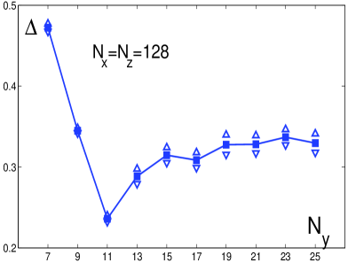
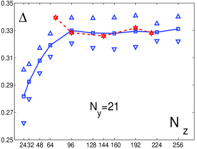
The experiment where $N_{y}$ is varied (left panel) is performed with $N_{x}=N_{z}=128$. Squares mark the time-averaged $\Delta$ and up/down triangles indicate the standard deviation of its fluctuations around the average. The experiment with variable $N_{x},N_{z}$ (right panel) assumes $N_{y}=21$. It reports two cases. The first one is with $N_{x}=N_{z}$ varying from 24 to 256, where the squares indicate the time-averaged $\Delta$ and up/down triangles the standard deviation as before. The second one is with $N_{z}=3N_{x}$ and the time-averaged $\Delta$ marked with stars, the corresponding standard deviation is the same order of magnitude and not shown for the sake of readability.

A clear convergence of the results is observed as the resolution is increased, marked by a plateau reached for $N_{y}\sim 15$ and $N_{x}=N_{z}\sim 96$. We are rather interested in the opposite limit of decreased resolution. Whereas a gentle trend is observed for $N_{y}\geq 11$, the cases $N_{y}=9$ and $7$ behave differently and a divergence in finite time is even observed for $N_{y}<7$. In fact, for the moderate Reynolds numbers of interest here, $N_{y}=11$ appears to be a bound below which the numerical solution is no longer physical. Figure 2

Figure 2: Colour level representations of the $x$ component of the velocity perturbation in the mid-plane $y=0$ of full three dimensional snapshots of the numerical solutions obtained in a domain $32\times 2\times 32$ for $R=450$ at $t=2000$. $N_{x}=N_{z}=128$ in-plane collocation points, and $N_{y}$ Chebyshev polynomials in the cross-stream direction, with $N_{y}$ ranging from 9 to 25. The $x$ and $z$ axes are respectively horizontal and vertical, like in all most of the other figures displaying patterns, except stated otherwise.

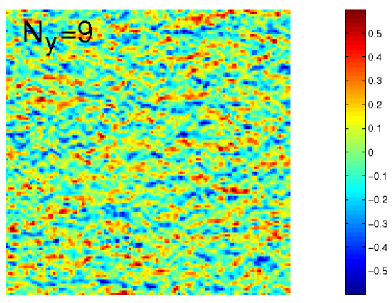
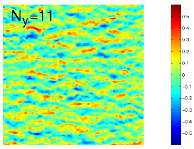
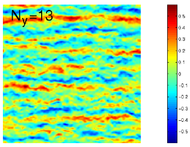
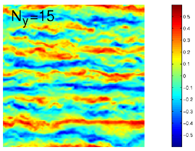
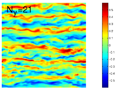
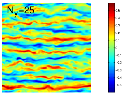
displays the streamwise component of the disturbance in the plane $y=0$. For $N_{y}=9$ the solution shows an anomalously fine in-plane structure, as if turbulent energy could only be dissipated by being transferred to structures with fast variations in $x$ and $z$. By contrast, the solutions obtained for $N_{y}\geq 11$ display coarser velocity fluctuations, the case $N_{y}=13$ being already qualitatively similar to those for $N_{y}=15$, $21$, and $25$. These patterns are reminiscent of the very large streamwise streaky turbulent structures obtained in wall-bounded flows [6, 7].

These structures can further be identified in Figure 3 which presents Fourier spectra of $u_{0}(t=2000)$ for the different resolutions considered. In all the graphs, the envelopes of the projections of the spectra are displayed, that is to say $\Sigma(k_{x})=\max_{k_{z}}S(k_{x},k_{z})$ and $\Sigma(k_{z})=\max_{k_{x}}S(k_{x},k_{z})$, where $S(k_{x},k_{z})=|\hat{u}_{0}|^{2}$ is the Fourier spectrum of $u_{0}$. The information contained in these quantities, though somehow limited, is more readable than the display of the full spectra while giving a proper account of the anisotropy of the flow that clearly distinguishes the spanwise and streamwise directions.

For variable $N_{y}$, Fig. 3 (top), the cases

Figure 3: Envelopes of Fourier spectra of the streamwise velocity component in the mid-plane $u_{0}$ for $L_{x}=L_{z}=32$, $R=450$, and a single snapshot at $t=2000$. Top: $N_{y}$ variable, $N_{x}=N_{z}=128$. Bottom: $N_{x}=N_{z}$ variable, $N_{y}=21$. Spectra are not scaled by the total number of modes $N_{x}N_{z}$. For the top line $N_{x}N_{z}$ is constant and spectra envelopes appear on top of each other, whereas for the bottom line the number of modes depend on the resolution so that they are shifted upward as it increases.

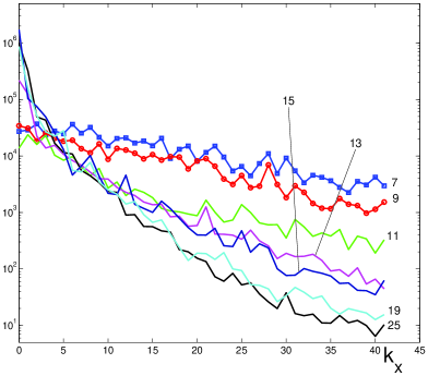
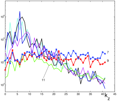
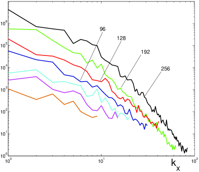
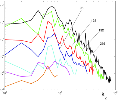
$N_{y}=7$ and $9$ are clearly not properly resolved since the envelopes of the projected spectra do not decay as $k_{x}$ and $k_{z}$ increase. Already present for $N_{y}=11$, the correct tendency strengthens as $N_{y}$ increases, though less rapidly in the streamwise direction than in the spanwise direction. Along the $k_{z}$ axis, except for $N_{y}=11$, a clear peak is observable for $k_{z}\sim 7$, i.e. $\lambda_{z}=L_{z}/7)\sim 4.6$; this value is somewhat larger than but of the same order of magnitude as the width $\ell_{z}$ of the MFU mentioned above. In contrast, no peak at finite $k_{x}$ is observed in the streamwise direction but a monotonic decrease as $k_{x}$ varies from zero to $k_{x,{\rm max}}=N_{x}/3$. These two features are in line with the observation of the very elongated streamwise streaky structures in wall-bounded flows. Similar trends are observed for $N_{y}=21$ and variable $N_{x}$ in Figure 3 (bottom) where the spectra appear shifted with respect to one another due to the absence of normalisation by the number of modes in order to improve the readability of the figure. The peak at $k_{z}\sim 7$ is visible for $N_{x,z}\geq 64$ but not at lower resolution which is not surprising when we compare the corresponding wavelength $L_{z}/7\approx 4.6$ and the effective space step $\delta_{x,z}^{\rm eff}$: for $N_{x,z}=48$, this makes $\delta_{x,z}^{\rm eff}=3L_{x,z}/2N_{x,z}=1$, hence less than five points per spanwise wavelength, which really does not seem to be enough.

Up to now we have not yet taken into account the fact that the velocity fluctuations vary much more rapidly in the spanwise direction than in the streamwise direction. Here we thus consider effective space steps systematically smaller by a factor of three along $z$ than along $x$, i.e., $N_{x}=N_{z}/3$. Results for $\Delta$ are shown in the right panel of Figure 1 as stars. Except for the lowest value $(N_{x},N_{z})=(24,72)$, all other values agree with those determined for $N_{x}=N_{z}$ when plotted as functions of $N_{z}$, which means that in-plane resolution can be appreciated from the value of $N_{z}$ alone with $N_{x}$ down to a factor of three smaller. This observation is confirmed by the examination of the envelope spectra as defined above shown in figure 4. Both $u_{0}$ and $v_{0}\equiv v(x,y=0,z;t)$ at $t=2000$ have been considered. Here the Fourier amplitudes have been normalised by the corresponding numbers of modes and it is clearly seen that they pile up for $N_{x}\geq 48$, $N_{z}\geq 144$, that is to say $\delta_{x}^{\rm eff}=3L_{x}/2N_{x}=1$ and $\delta_{z}^{\rm eff}=3L_{z}/2N_{z}=0.33$.

Figure 4: Fourier spectra of the streamwise ($u$) and wall-normal ($v$) corrections to the laminar profile for the turbulent flow at $R=450$, evaluated at $y=0$ ($L_{x}=L_{z}=32$, single snapshot at $t=2000$, $N_{y}=21$ and $N_{z}=3N_{x}$ variable). Top: streamwise perturbation $u$. Bottom: wall-normal perturbation $v$. Left: streamwise component $k_{x}$. Right: spanwise component $k_{z}$. Successively: $(N_{x},N_{z})=$ $(24,72)$, $(32,96)$, $(48,144)$, $(64,192)$, and $(72,216)$. All spectra rescaled by $N_{x}N_{z}$ in order to show how well they pile up.

Figure 5: Profiles of $\bar{\Delta}(y)$ as functions of the wall-normal resolution $N_{y}$ as interpolated from values at collocation points using cubic splines. Left: lowest resolution, $N_{y}$ from 7 to 13. Right: highest resolutions, $N_{y}$ from 13 to 25. ($L_{x}=L_{z}=32$, $N_{x}=N_{z}=128$, $R=450$, $t=2000$.)

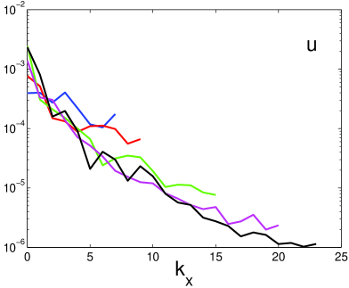
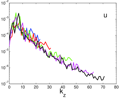
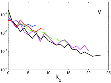
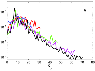
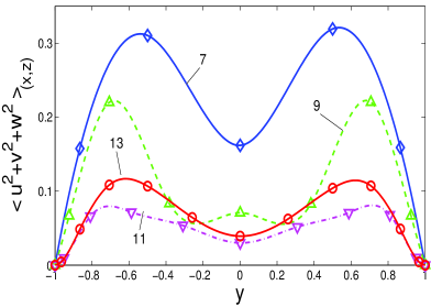
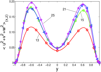
How well the turbulent regime is reproduced in low resolution simulations has also been tested by comparing in-plane averaged profiles of the streamwise velocity correction $\bar{u}(y)=(1/L_{x}L_{z})\int u(x,y,z)\,{\rm d}x\,{\rm d}z$ and the squared distance to the base solution $\bar{\Delta}(y)=(1/L_{x}L_{z})\int(u^{2}+v^{2}+w^{2})\,{\rm d}x\,{\rm d}z$. Figure 5 displays the latter quantity for a series of experiments with $N_{y}$ varying from 7 to 25. Results for $\bar{u}(y)$ are similar. No averaging over time has been performed: a single snapshot at $t=2000$ has been used in each case, which explains possible irregularities and a slight lack of $y$-symmetry for $N_{y}=15$ and 21. From the figure, one can immediately see that profiles for $N_{y}=7$ and 9 are off, that those for $N_{y}=11$ and $13$ progressively evolve so as to tend toward a limiting profile, and that consistent results are obtained for $N_{y}\geq 15$ in agreement with observations already made when considering Figure 1 (left).

3 Decreasing the numerical resolution: quantitative effect on the bifurcation diagram

This preliminary study suggests that the featureless turbulent regime is reasonably well rendered provided that $N_{y}\geq 15$ and effective in-plane resolution $\delta_{x}^{\rm eff}=3L_{x}/2N_{x}\leq 1$ and $\delta_{z}^{\rm eff}=3L_{z}/2N_{z}\leq 0.33$. It remains to test the effect of a lowering of the resolution on the peculiarities of the ‘turbulent$\to$laminar’ transition via oblique turbulent bands, which is done in the present section.

According to the experiments [1], the pattern can be characterised by a wavevector $\mathbf{k}^{\rm patt}$ with components $k_{x}^{\rm patt}=2\pi/\lambda_{x}$ and $k_{z}^{\rm patt}=2\pi/\lambda_{z}$. Furthermore, $\lambda_{x}\simeq 110$ is obtained all along the transitional range and $\lambda_{z}$ varies from $50$ for $R=395$ close to the top at $R_{\rm t}\simeq 410$, to $82$ at $R=340$ when the bands break down into patches that finally decay below $R_{\rm g}\simeq 325$. Wishing to perform simulations in wide domains at the lowest possible computational cost, we now validate our modelling strategy by examining the effect of a lowering of the resolution on the bifurcation diagram in extended domains of size sufficient to fit at least about one streamwise wavelength $\lambda_{x}$ and one spanwise wavelength $\lambda_{z}$ of the band pattern. Accordingly, we consider rectangular domains of size $L_{x}\times L_{z}$ with $L_{x}\geq 110$ and $L_{z}\geq 50$. Except for $N_{y}=7$ and $9$, oblique bands are obtained without any difficulty in a full range of Reynolds numbers.

Experiments are all done under the same protocol: a featureless turbulent regime is prepared at $R=450$ and $R$ is next decreased by steps. At every value of $R$, the simulation is pursued sufficiently long for the establishment of statistical equilibrium before further decreasing $R$. Usually, this takes at least 5000 time units. The distance $\Delta$ is recorded as a function of time. After elimination of a transient just after the change in $R$, its time average and the rms value of its fluctuations are computed.

The result of the experiment for $N_{y}=21$, $(L_{x},L_{z})=(110,84)$ and $(N_{x},N_{z})=(440,336)$, shown in Figure 6 (left), is typical.

Figure 6: Left: Time-averaged quantity $\Delta$ as a function of $R$ for $N_{y}=21$ with $(L_{x},L_{z})=(110,84)$ and $(N_{x},N_{z})=(440,336)$. Right: Thresholds $R_{\rm g}$ and $R_{\rm t}$ as functions of the number $N_{y}$ of Chebyshev polynomials for different in-plane resolutions and domain sizes, see text.

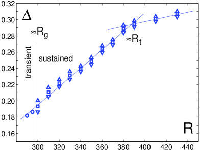
This figure displays, as functions of $R$, the time averages of $\Delta$ as squares and the standard deviations of fluctuations as up/down triangles. (Estimates for transient states observed below $R_{\rm g}$ are shown as open circles, see below.)

A break in $\Delta$ as a function of $R$ is identified as the upper threshold $R_{\rm t}$. Visually, this break corresponds to the appearance of regions where the turbulence intensity is depleted. A continuous diagonal band forms as $R$ is decreased below $R_{\rm t}$, which, once periodically continued in the spanwise and streamwise directions features the expected oblique pattern. The decrease of $\Delta$ which measures the average distance to the laminar profile is easily understood as the result of a decrease of the turbulent fraction, the ratio of the surface of the region still turbulent to the total surface of the system. This fraction is determined by thresholding the local mean perturbation kinetic energy $\bar{E}_{\rm t}(x,z;t)$. In their simulations, Barkley & Tuckerman [8] observe that the turbulent intensity is larger inside turbulent bands than in the featureless regime. Quantity $\Delta$ being an average over the whole domain, by compensation this could lead to an underestimation of $R_{\rm t}$. Rather than trying to correct for this intensification effect we choose to define $R_{\rm t}$ as given by the position of the break further confirmed by visual inspection of the flow pattern.

The second limit $R_{\rm g}$ is determined as the value of $R$ below which turbulence decays in less than 10000 time units. This value is obtained from a single experiment, but a rapid change within a small interval in $R$ is observed between sustained banded turbulence with limited fluctuations of $\Delta$ and a turbulent regime bound to decay which displays large excursions toward values of $\Delta$ well below the average. Below $R_{\rm g}$, taking the mean of $\Delta$ during the plateau that precedes the final decay produces the measurements displayed as open circles which appear to be well aligned with the other points corresponding to sustained turbulence.

At any rate our aim here is not to perform a detailed statistical study of transient turbulence as in previous studies [5] but to locate $R_{\rm t}$ and $R_{\rm g}$ approximately as a function of the resolution. A very conservative estimate of the precision with which $R_{\rm t}$ and $R_{\rm g}$ are determined is $\pm 5$, which meets our purpose.

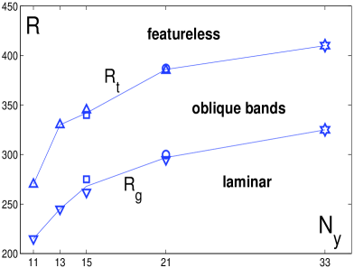
The results of the most systematic study with $(L_{x},L_{z})=(128,64)$, $(N_{x},N_{z})=(512,256)$ are displayed in Figure 6 (right) as up-triangles for $R_{\rm t}$, down-triangles for $R_{\rm g}$. Values at $N_{y}=33$, marked with hexagrams, are taken from the literature [9], in close agreement with experimental observations [1]. The bifurcation diagram shows a regular shift of the interval in $R$ where bands are observed. These results do not depend on the precise size of the domain provided that it is sufficiently large to accommodate a band, as seen from a comparison of the results for $L_{x}=128$ and $L_{z}=64$ with those from the experiment with $L_{x}=110$ and $L_{z}=84$ described above and reported as open circles at $N_{y}=21$. They are also not so sensitive to the in-plane resolution, as seen from the results at $N_{y}=15$ of the ‘high’-resolution experiment with $(N_{x},N_{z})=4\times(L_{x},L_{z})$ compared to those of a ‘low’-resolution control experiment with $N_{x}=L_{x}$ and $N_{z}=3L_{z}$ displayed as open squares. A similar shift was observed by Willis and Kerswell in the pipe flow case though in the opposite direction of increased thresholds [14]. However, in their case, the resolution decrease was in the azimuthal direction, which corresponds to our spanwise direction. This difference is likely to play a role on the turbulence sustenance mechanisms, so that no definite inference can be made from this observation.

Corroborating the observation of an anomalous behaviour of the fully turbulent state for $N_{y}=7$ and $9$ (Fig. 1, left; Fig. 2, top-left), banded patterns are not obtained in these cases. On the contrary, a continuous decrease of $\Delta$ is observed as $R$ is decreased. For $N_{y}=9$, a featureless turbulent state similar to that at $R=450$ (Figure 2, top-left) can indeed be maintained as low as $R=185$ while for smaller $R$, a small-scale streamwise structure happens to grow on top of a large scale spanwise modulation of the turbulence intensity. This manifestly non-physical, slowly time-dependent, numerical solution finally decays abruptly as the Reynolds number is further decreased but a detailed study of this transition is pointless. Similarly, an even more exotic but equally uninteresting chaotic state is obtained for $N_{y}=7$, and maintained at even lower $R$.

A caveat is however required: at moderate (i.e. not the lowest) resolution, spurious stable nontrivial nearly-steady states can be found at values of $R$ in the lower part of the range where the bands exist and below, in the form of localised states resembling edge states, e.g. [17]. An example is shown in Figure 7 (left).

local mean perturbation energy

streamwise perturbation velocity component $u$

Figure 7: Left: Spurious ‘edge state’-like numerical solution for $N_{y}=19$ close to the saddle-node bifurcation point $R\approx 309.5$ ($L_{x}=110$, $L_{z}=32$, $N_{x}=440$, $N_{z}=128$); this solution is mostly concentrated in the upper half of the channel ($y>0$) as understood from the comparison of the variation ranges of $vx\equiv u(x,y,z,t)$ for $y=+0.766$ and $y=-0.766$ at steady state ($t\to\infty$); Right: Variation of the saddle-node threshold $R_{\rm sn}$ as a function of $N_{y}$ for the family of spurious numerical solutions.

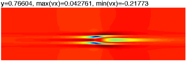
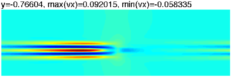
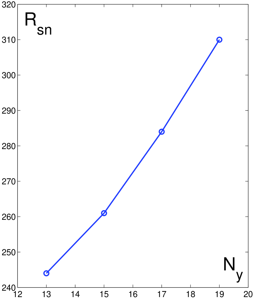
As understood from the display of the local mean perturbation energy and the streamwise component of the perturbation velocity, this solution has broken the symmetries of the plane Couette flow since it is predominantly localised in $y\in[0,1]$ and not symmetrically distributed over $[-1,1]$. As a result of the symmetry breaking, this localised state moves slowly in the streamwise direction. The resolution being given, such a state can be viewed as a solution to some dynamical system and, so, belonging to some solution branch along which it can bifurcate as $R$ is varied. It turns out that this state exists in a limited range between a lower saddle-node threshold where it disappears and an upper threshold where it experiences a Hopf bifurcation, and next nucleates a turbulent spot, which is expected and thus not studied in detail. In fact, this solution belongs to a family that exists for a range of cross-stream resolutions $N_{y}$. It was obtained from another one obtained during the decay of a turbulent state for $N_{y}=15$ and $R=270$, then carried to $N_{y}=13$ on the one hand, and to $N_{y}=17$ and next $N_{y}=19$ on the other hand, but could be stabilised neither for $N_{y}=11$ nor for $N_{y}=21$. Figure 7 (right) displays the threshold of the saddle-node bifurcation through which this solution family disappears. This threshold is seen to increase rapidly and to lie below $R_{\rm g}$ for $N_{y}=13$ or 15, and above for $N_{y}=19$, which is probably the reason why we cannot find it for $N_{y}=21$ without the help of a sophisticated continuation procedure. This family of spurious solutions is most probably not unique. Unlike genuine edge states that are unstable by construction and proposed to represent gates on the boundary of attraction basin of the base flow, they are stable at least within some range of Reynolds numbers; the mechanisms by which they are maintained should however be essentially identical. We stress that this unwanted side effect of under-resolution here acts on nontrivial but non-chaotic states and is not expected to spoil our study of turbulent regimes which are sensitive to noise inherent in chaos but statistically robust enough to withstand perturbations due to truncation errors.

To conclude this section, in spite of the caveat above, evidence has been given that as long as unsteady (turbulent) states are considered, reducing the wall-normal resolution is a viable modelling strategy. Of course the best possible resolution is desirable but, in view of a quantitative reproduction of the transitional range of plane Couette flow, we can recommend that the number $N_{y}$ of Chebyshev polynomials be kept larger than or equal to 11, whereas a tolerable shift of the upper and lower bounds of that range is obtained provided that $N_{y}\geq 15$. In-plane resolutions with $N_{x}\geq L_{x}$ and $N_{z}\geq 3L_{z}$ also appear satisfactory, with corresponding numbers of Fourier modes $\frac{2}{3}N_{x,z}$.

4 Discussion

We begin by presenting preliminary results obtained in parallel with the study presented above to illustrate how it can be used, before making more general comments on the numerical approach to transitional wall-bounded flows.

$\bullet$ Extreme case.

The emergence of turbulent bands first appears to be an extremely robust phenomenon. Here we show simulation results in the most extreme conditions that we have considered, namely $N_{y}=11$ and $N_{x}=L_{x}$, $N_{z}=L_{z}$. The lateral size of the domain is $L_{x}=682$ and $L_{z}=381$, which is already larger than in the early Saclay experiments [18] and of the same order of magnitude as in the latest experiments [1] or the simulations reported in [9] but with the computation power of a desk-top computer. From results in Fig. 6 (right), we expect $R_{\rm t}\simeq 270$ and $R_{\rm g}\simeq 215$. Quench experiments similar to those of Bottin [18] are performed. Results are displayed in Figure 8.

Figure 8: Quench experiment for $N_{y}=11$, $N_{x}=L_{x}=682$, $N_{z}=L_{z}=341$. Top: Time series of quantity $\Delta$ for the values of $R$ indicated. Bottom, from left to right and top to bottom: Snapshots of pattern obtained in the different asymptotic regimes obtained at $t=4000$ after the quench for $R=250$ (continuous bands), $R=240$ (interrupted bands), $R=237$ (border state), and at $t=500$ for $R=235$ (decaying spots).

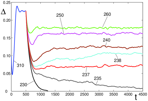
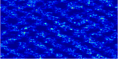
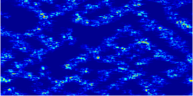
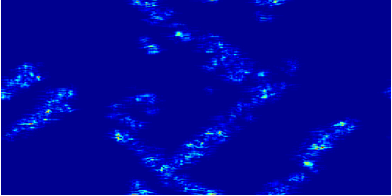
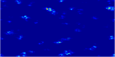
A turbulent state is prepared at $R=310\gg R_{\rm t}$. At time $t=500$, $R$ is suddenly reduced to some final value $R_{\rm f}$. Time series of the quantity $\Delta$ are shown in the top panel. Snapshots of the solution are taken at regular times. The experiment is stopped at $t=4000$ after the quench or when the laminar state is recovered.

After the quench, a fast drop of $\Delta$ is observed with a pronounced undershoot for $R=260$, $250$, and $240$. During the drop, the evolution amounts to a general, more or less uniform, breakdown of the turbulent state that, when the minimum is reached, leaves a few turbulent patches of limited extent. The turbulent fraction then re-increases and bands form. For $R=260$ and $250$ continuous bands are obtained but, in contrast with experiments where a single wave vector $\mathbf{k}^{\rm patt}$ was selected, here two wavevectors symmetrical with respect to the streamwise direction ($\pm k_{z}$) dominate the pattern as displayed in the top-left image. The quench at $R_{\rm f}=240$ ends with a regime where bands are fragmented in the top-right image. For smaller $R_{\rm f}$, the undershoot is less pronounced and the recovery stage slower. The asymptotic regime reached at $R=237$ will be called a border state since—within the quench protocol—it sits on the frontier separating decaying from sustained regimes. As such, arguably, it could have been called an ‘edge state’ but this term has been already extensively used in the study of the transition in terms of dynamical systems [5] which focuses of the temporal dynamics of localised structures that are exceptional limit sets. In contrast, the state shown in the bottom-left image appears typical of the spatiotemporal aspects of the transition. For $R_{\rm f}=230$, the system does not recover and the turbulent patches decay immediately. Apart from an important downward shift of $R_{\rm t}$ and $R_{\rm g}$, all of the observed scenario is identical to results described by Duguet et al. [9] obtained in a much better resolved context, or to Prigent’s experiments [1].

From the above one could conclude that $R_{\rm g}\approx 237$, which is somewhat larger than the value obtained using the adiabatic protocol used to obtain Figure 6 (right) in which one gets $R_{\rm g}\approx 215$. This discrepancy might be due to the difference in the in-plane resolution: $N_{x,z}=4L_{x,z}$ for results in that figure vs. $N_{x,z}=L_{x,z}$ here. A similar effect was already apparent for $N_{y}=15$ and the two resolutions considered: $R_{\rm g}\simeq 262$ was obtained with $N_{x,z}=4L_{x,z}$ (down triangle) and $R_{\rm g}\simeq 275$ with $N_{x}=L_{x}$, $N_{z}=3L_{z}$ (square), which is slightly better than now ($N_{z}=L_{z}$). Another, more likely, explanation can also be found in the fact that the threshold obtained in the quench experiment is only an upper bound to $R_{\rm g}$: The quench protocol always involves a recovery stage starting at the end of the undershoot. The corresponding state is an assembly of turbulent spots similar to what is pictured in figure 8 (bottom, right) during the early decay at $R=235$. In this respect, the quench experiment is an initial value problem similar to that of Duguet et al. [9], or to any experiment in which spots are triggered. In contrast, the adiabatic decrease of $R$ is the sole protocol supposed to yield, by continuation, the global stability threshold defined as the lowest value of $R$ above which sustained turbulence has a non-empty attraction basin. Except in a well-conducted adiabatic experiment, this attraction basin may indeed be hard to find until one reaches values of $R$ where it has a sizeable breadth, which is somewhat beyond $R_{\rm g}$.

The superposition of two sets of bands illustrated above instead of one, as expected from the experiments, is also the result of a resolution which, though qualitatively satisfactory, is nevertheless too poor since ongoing simulations with $N_{y}=15$ show a single dominant wavevector in the range of Reynolds numbers corresponding to bands. Interpreting the result in terms of pattern formation and Ginzburg–Landau envelope equations [1], when the resolution is low ($N_{y}=11$) the coefficient of the cubic term $|A_{\mp}|^{2}A_{\pm}$ accounting for the interaction between wavevectors $+k_{x}$ and $-k_{x}$ (explicitly defined in the next paragraph) is under-estimated compared to the coefficient of the term $|A_{\pm}|^{2}A_{\pm}$ accounting for self-interaction, so that each orientation can develop to form a rhombic pattern; a ratio compatible with experimental findings is restored by increasing the resolution, ending in a stripe pattern ($N_{y}=15$). On the other hand, it should be stressed that, despite the constraints brought by the periodic boundary conditions, the pattern’s wavelengths and their variation are correctly reproduced since we can measure $\lambda_{x}\approx 114=L_{x}/6$ (and not $L_{x}/5=136$ nor $L_{x}/7=97$) for both $R=250$ and $240$ and $\lambda_{z}=68\>(=L_{z}/5)$ and $85\>(=L_{z}/4)$ for $R=250$ and $240$, respectively.

$\bullet$ A better resolved experiment.

The case considered above stays too close to the boundary of the basin where DNS faithfully accounts for transitional plane Couette flow. The real motivation of our work is to consider less extreme simulation conditions in view of a quantitatively better rendering of the different regimes observed. With our present computational capabilities, this can only be done by increasing $N_{y}$ while simultaneously keeping a sufficiently high in-plane resolution at the expense of decreasing the size of the domain. Accordingly we have considered a system of size sufficient to afford at least a full elementary cell of the experimentally observed pattern, i.e. $L_{x}\sim\lambda_{x}$ and $L_{z}\sim\lambda_{z}$. The example shown here is with $L_{x}=110$ and $L_{z}=84$ and a resolution $N_{y}=15$, $N_{x}=512$, $N_{z}=256$. It aims at the identification of an appropriate order parameter for the pattern [19]. The top row of Figure 9

Figure 9: Four snapshots of the solution for $R=315$ ($N_{y}=15$, $L_{x}=110$, $N_{x}=512$, $L_{z}=84$, $N_{z}=256$, $x$ axis is vertical). Bottom: Time series of the amplitude of the different dominant Fourier modes.

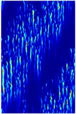
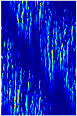
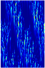
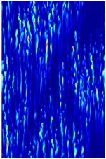
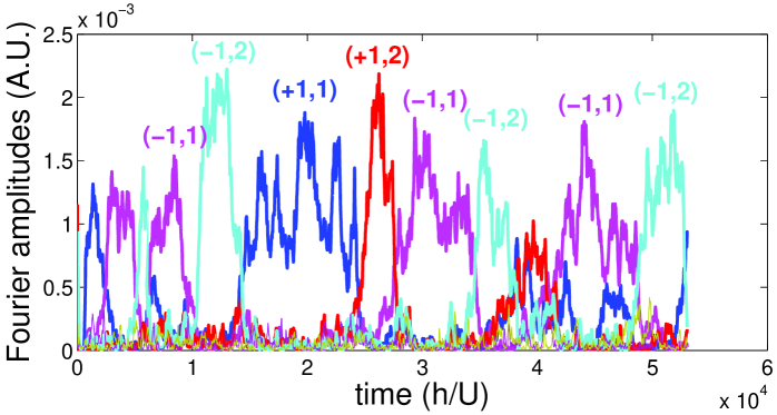
displays snapshots of the local mean energy at different times during a long simulation at $R=315$. Band patterns with a single band leaning to the right or to the left, with two bands leaning to the left, or a messy situation, can be observed. Fourier analysis then yields either one dominant mode (well formed patterns, Fig. 9, left and centre) or several interacting modes (defective pattern, Fig. 9, right). In the present context, Fourier amplitudes are good candidates to play the role of order parameters. They were indeed considered by Barkley et al. in [8] and [20]. The time series of the Fourier amplitudes shown as functions of time in Figure 9 (bottom) indicate an apparently random alternation of states that can be characterised by a dominant mode ($\pm$ indicate left or right, and 1 or 2 the number of bands, i.e. $k_{x}=\pm 2\pi n_{x}/L_{x}$ and $k_{z}=2\pi n_{z}/L_{z}$, with $n_{x}=1$ and $n_{z}=1,2$). Preliminary analysis suggests that the sojourn times in one or another state are exponentially distributed, which suggests an approach in terms of a stochastic multi-well process. This interpretation follows from the probable existence of a Landau potential with minima appropriate to describe the several possible pattern configurations, and the presence of a permanent excitation due to the noise generated by turbulence [1]. But, to be validated, such an interpretation requires large amounts of data still being gathered in different conditions in order to get the variation of the order parameter, its mean value and standard deviation, as functions of $R$ for different aspect-ratios $L_{x,z}$.

$\bullet$ Final remarks.

When combined with the reliability assessment provided in Sections 2 and 3, these preliminary results bring an interesting contribution to the phenomenology of plane Couette flow at minimal numerical cost. The pattern’s main characteristics are recovered. Turbulent band formation appears to be a robust feature in the transitional range $R\>\in\>[R_{\rm g},R_{\rm t}]$. The order of magnitude of the pattern’s wavelengths and their variations with $R$ are also well reproduced in the simulations, even at the lowest possible resolution. The price to be paid for the resolution decrease just seems to be a regular shift of the transitional range toward lower Reynolds numbers.

These results also illustrate the specifically spatiotemporal features of the transitional range. In particular, turbulence decay may not well be rendered by the temporal approach implemented in low-dimensional dynamical systems theory (chaotic transients [5]). The latter approach remains adapted to chaotic but spatially coherent dynamics in domains a few MFUs wide. It can be of use to understand the nucleation of laminar patches of limited extent within featureless turbulence. It is however unable to account for the regular regression of turbulent domains coexisting with laminar flow which marks the decay stage in large aspect ratio systems, either in the laboratory or in the computer. This is attested by the variation of $\Delta$ shown here for $R=235$ and $N_{y}=11$ in Fig. 8, but typical of better resolved cases.

Interesting results have already be obtained in an elongated inclined domain [8, 20] but confinement by periodic boundary conditions in the direction parallel to the short side perturbs the long-range streamwise coherence of the streaks (Fig. 2). This warrants further study and leads us to suggest that one should consider domains that are at least as large as one elementary cell $(\lambda_{x},\lambda_{z})$ of the band pattern.

As a modelling strategy within the extended systems perspective, results presented here drastically improves over the model previously elaborated in [11] and used in [12]. Though that model is amenable to analytic treatment in view of the elucidation of the mechanisms producing the experimentally observed turbulence modulation, the present numerical findings point out the role of its effective cross-stream resolution which is much too low. On the other hand, the fact that limited resolution reproduces the main features of the dynamics of the flow in the transitional range suggests that the observed pattern formation does not involve processes taking place in a thin boundary layer close to the plates where high-order cross-stream modes are of importance, but larger scale interactions in the bulk of the shear where structures controlled by moderate-order modes operate (see [21] for the companion problem of puff sustainment in pipe flow). This observation could motivate the search for a model of intermediate complexity along the lines traced in [11] by pushing the Galerkin expansion a little further in view of an analytical approach.

To conclude, plane Couette flow presents itself as an academic prototype of wall-bounded flows, with the extreme condition that it is linearly stable for all $R$, forcing its subcritical character. Low resolution simulations allows numerical experiments at minimal cost in circumstances where dynamics in physical space becomes more relevant (laminar/turbulent coexistence) than in phase space where the collection of competing exact solutions becomes increasingly large and their properties difficult to exploit. Our unorthodox approach of decreasing the resolution in a controlled way may be considered as a modelling methodology which will allow refined statistics, in view of Pomeau’s thermodynamic analogy [15, 22], and help to pose appropriate questions about the physics behind band formation. The approach can certainly not be extended to the fully developed regime nor to initial spot development where high resolution is an important issue, but moderately turbulent regimes involved in the transitional range of less academic flows could take advantage of it when the lateral extension is of primordial interest.

Acknowledgements: P.M. wants to thank Y. Duguet and G. Kawahara for interesting discussions related to this work, and the latter for his invitation to present it in Osaka. Helpful comments of a referee are also deeply acknowledged.

References

- [1] Prigent A. et al.: Long-wavelength modulation of turbulent shear flows. Physica D 174, 100–113 (2003).
- [2] Andereck, C.D., Liu, S.S., Swinney, H.L.: Flow regimes in a circular Couette flow system with independently rotating cylinders. J. Fluid Mech. 164 155–183 (1986).
- [3] Jimenez, J., Moin, P.: The minimal flow unit in near wall turbulence. J. Fluid Mech. 225 213–240 (1991).
- [4] Hamilton, J.M., Kim, J., Waleffe, F.: Regeneration mechanisms of near-wall turbulence structures. J. Fluid Mech. 287 317–348 (1995).
- [5] Eckhardt, B., Faisst, H., Schmiegel, A., Schneider, T.M.: Dynamical systems and the transition to turbulence in linearly stable shear flows, Phil. Trans. R. Soc. A 366 1297–1315 (2008).
- [6] Komminaho, J., Lundbladh, A., Johansson, A.J.: Very large structures in plane turbulent Couette flow. J. Fluid Mech. 320 259–285 (1996).
- [7] McKeon, B.J., Sreenivasan, K.R. (eds.): Scaling and structure in high Reynolds number wall-bounded flows. Focus Issue, Phil. Trans. R. Soc. A 365 (2007).
- [8] Barkley, D., Tuckerman, L.S.: (a) Computational study of turbulent laminar patterns in Couette flow. Phys. Rev. Lett. 94 014502 (2005). (b) Turbulent-laminar patterns in plane Couette flow. In: Mullin, T., Kerswell, R. (eds.): IUTAM symposium on laminar-turbulent transition and finite amplitude solutions. Springer, Dordrecht (2005). (c) Mean flow of turbulent-laminar patterns in plane Couette flow. J. Fluid Mech. 576 109–137 (2007).
- [9] Duguet, Y., Schlatter, Ph., Henningson, D.S.: Formation of turbulent patterns near the onset of transition in plane Couette flow. J. Fluid Mech. 650 119–129 (2010).
- [10] Tsukahara, T., Kawaguchi, Y., Kawamura, H.: DNS of turbulent plane Couette flow with emphasis on turbulent stripes. In: Eckhardt, B. (ed.): Advances in Turbulence 12, Springer, Dordrecht (2009) pp. 71–74.
- [11] Lagha, M., Manneville, P.: Modeling transitional plane Couette flow. Eur. Phys. J. B 58 433–447 (2007).
- [12] Manneville, P.: Spatiotemporal perspective on the decay of turbulence in wall-bounded flows. Phys. Rev. E 79 (2009) 025301 [R]; 039904 [E].
- [13] Waleffe, F.: On a self-sustaining process in shear flows. Phys. Fluids 9 883–900 (1997).
- [14] Willis, A., Kerswell, R.R.: Turbulent dynamics of pipe flow captured in a reduced model: puff relaminarisation and localised ‘edge’ state. J. Fluid Mech. 619 213–233 (2009).
- [15] Pomeau, Y.: Front motion, metastability and subcritical bifurcations in hydrodynamics. Physica D 23 (1986) 3-11.
- [16] J. Gibson. http://www.channelflow.org/.
- [17] Duguet, Y., Schlatter, Ph., Henningson, D.S.: Localized edge states in plane Couette flow Phys. Fluid 21 (2009) 111701.
- [18] (a) Bottin, S., Dauchot, O., Daviaud, F., Manneville, P.: Discontinuous transition to spatiotemporal intermittency in plane Couette flow. Europhys. Lett. 43 171–176 (1998). (b) Bottin, S., Chaté, H.: Statistical analysis of the transition to turbulence in plane Couette flow. Eur. Phys. J. B 6, 143–155 (1998).
-
[19]
Rolland, J., Manneville, P.:
Oblique turbulent bands in plane Couette flow: From visual to
quantitative data,
16th International Couette–Taylor Workshop, Princeton University,
September 2009. Ji Hantao, Smits, L. (eds.)
http://www.princeton.edu/~asmits/ICTW/PROGRAM-Sep06.pdf - [20] Tuckerman, L.S., Barkley, D., Dauchot, O.: Instability of uniform turbulent plane Couette flow: spectra, probability distribution functions and closure model. Schlatter, Ph., Henningson, D.S. (eds.): 7th IUTAM Symposium on laminar-turbulent transition, Stockholm, June 2009. Springer (2010).
- [21] Shimizu, M., Kida, S.: A driving mechanism of a turbulent puff in pipe flow. Fluid Dyn. Res. 41 (2009) 045501.
- [22] Pomeau, Y.: Chapitre IV, Transition vers la turbulence dans les écoulements parallèles. In: Bergé, P., Pomeau, Y., Vidal, Ch.: L’espace chaotique. Hermann, Paris (1998).