Hierarchical Multiclass Decompositions with Application to Authorship Determination

Abstract

This paper is mainly concerned with the question of how to decompose multiclass classification problems into binary subproblems. We extend known Jensen-Shannon bounds on the Bayes risk of binary problems to hierarchical multiclass problems and use these bounds to develop a heuristic procedure for constructing hierarchical multiclass decomposition for multinomials. We test our method and compare it to the well known “all-pairs” decomposition. Our tests are performed using a new authorship determination benchmark test of machine learning authors. The new method consistently outperforms the all-pairs decomposition when the number of classes is small and breaks even on larger multiclass problems. Using both methods, the classification accuracy we achieve, using an SVM over a feature set consisting of both high frequency single tokens and high frequency token-pairs, appears to be exceptionally high compared to known results in authorship determination.

1 Introduction

In this paper we consider the problem of decomposing multiclass classification problems into binary ones. While binary classification is quite well explored, the question of multiclass classification is still rather open and recently attracted considerable attention of both machine learning theorists and practitioners. A number of general decomposition schemes have emerged, including ‘error-correcting output coding’ (SejnowskiR87; DietterichB95), the more general ‘probabilistic embedding’ (DekelS02) and ‘constraint classification’ (HarpeledRZ02). Nevertheless, practitioners are still mainly using the infamous ‘one-vs-rest’ decomposition whereby an individual binary “soft” (or confidence-rated) classifier is trained to distinguish between each class and the union of the other classes and then, for classifying an unseen instance, all classifiers are applied and the winner classifier, with the largest confidence for one of the classes, determines the classification. Another less commonly known method is the so called ‘all-pairs’ (or ‘one-vs-one’) decomposition proposed by (Friedman96). In this method we train one binary classifier for each pair of classes. To classify a new instance we run a majority vote among all binary classifiers. The nice property of the “all-pairs” method is that it generates the easiest and most natural binary problems of all known methods. The weakness of this method is that there may be irrelevant binary classifiers which participate in the vote. A number of papers provide evidences that ‘all-pairs’ decompositions are powerful and efficient and in particular, they outperform the ‘one-vs-rest’ method; see e.g. (Furnkranz02).

For the most part, known decomposition methods including all those mentioned above are “flat”. In this paper we focus on hierarchical decompositions. The incentive to decompose a multiclass problem as a hierarchy is natural and can have at the outset general advantages which are both statistical and computational. Considering a multiclass problem with $k$ classes, the idea is to learn a full binary tree of classes, where each node is associated with a subset of the $k$ classes as follows: Each of the $k$ leaves is associated with a distinct class, and each internal node is associated with the union of the class subsets of its right and left children. Each such tree defines a hierarchical partition of the set of classes and the idea is to train a binary classifier for each internal node so as to discriminate between the class subset of the right child and the class subset of the left child. Note that in a full binary tree with $k$ leaves there are $k-1$ internal nodes.

Once these tree classifiers are trained, the classification or “decoding” of an new instance can be done using various approaches. One natural decoding method would be to use the tree in a decision-tree fashion: Start with the binary classifier at the root and let this classifier determine either its right or left child, and this way follow a path to a leaf and assign the class associated with this leaf. This approach is particularly convenient when using hard binary classifiers giving labeles in $\{\pm 1\}$. When using “soft” (confidence-rated) and in particular probabilistic classifiers, giving confidence rates in $[0,1]$, a natural decoding method would be to calculate an estimate for the probability of following the path from the root to each leaf and then use a “winner-takes-all” approach, which selects the path with the highest probability.

Besides computational efficiency, the success of any multiclass decomposition scheme depends on (at least) two interrelated factors. The first factor is the statistical “hardness” of each of the individual binary classification problems. The second factor is the statistical robustness of the aggregation (or “decoding”) method. The most fundamental measure for the hardness of a classification problem is its Bayes error. We attempt to use the Bayes error of the resulting decomposition and aim to hierarchically decompose the multiclass problem so as to construct statistically “easy” collection of binary problems.

Determining the Bayes error of a classification problem based on the data (and without knowledge of the underlying distributions) is a hard problem, without any restrictions (LowerAntosDG99). In this paper we restrict ourselves to settings where the underlying distributions can be faithfully modelled as multinomials. Potential application areas are classification of natural language, biological sequences etc. We can therefore in principle conveniently rely on studies, which offer efficient and reliable density estimation for multinomials (ristad95natural; friedman99efficient; llester00convergence; griths-using). As a first approximation, throughout this paper we make the assumption that we hold “ideal” data smaples and simply rely on maximum likelihood estimators that count occurrences.

But even if the underlying distributions are known, a faithful estimation of the Bayes error is computationally difficult. We rely on known information theoretic bounds on the Bayes error, which can be efficiently computed. In particular, we use Bayes error bounds in terms of the Jansen-Shannon divergence (Lin91) and we derive upper and lower bounds on the inherent classification difficulty of hierarchical multiclass decompositions. Our bounds, which are tight in the worst case, can be used as optimality measures for such decompositions. Unfortunatelly, the translation of our bounds into provably efficient algorithms to search for high quality decompositions appear at the moment computationally difficult. Therefore, we use a simple and efficient greedy heuristic, which is able to generate reasonable decompositions.

We provide initial empirical evaluation of our methods and test them on multiclass problems of varying sizes in the application area of ‘authorship determination’. Our hierarchical decompositions consistently improve on the ‘all-pairs’ method when the number of classes are small but do not outperform all-pairs with larger number of classes. The authorship determination set of problems we consider is taken from a new benchmark collection consisting of machine learning authors. The absolute accuracy results we obtain are particularly high compared to standard results in this area.

2 Preliminaries: Bounds on the Bayes Error and the Jensen-Shannon Divergence

Consider a standard binary classification problem of classifying an observation given by the random variable $X$ into one of two classes $C_{1}$ and $C_{2}$. Let $\pi_{1}$ and $\pi_{2}$ denote the priors on these two classes, $\pi_{1}+\pi_{2}=1$ with $\pi_{i}\geq 0$. Let $p_{i}(x)=p(X=x|C_{i})$, $i=1,2$, be the class-conditional probabilities. If $X=x$ is observed then by Bayes rule the posterior probability of $C_{i}$ is $p(C_{i}|x)=\frac{\pi_{i}p_{i}(x)}{\pi_{1}p_{1}(x)+\pi_{2}p_{2}(x)}$. If all probabilities are known we can achieve the Bayes error by choosing the class with the larger posterior probability. Thus, the smallest error probability is

$$p(error|x)=\frac{\min\{\pi_{1}p_{1}(x),\pi_{2}p_{2}(x)\}}{\pi_{1}p_{1}(x)+\pi_{2}p_{2}(x)},$$

and the Bayes error is given by $p_{Bayes}=p(error)=\int_{x}p(x)p(error|x)dx=E_{x}[\min\{\pi_{1}p_{1}(x),\pi_{2}p_{2}(x)\}]$.

The Bayes error quantifies the inherent difficulty of the classification problem at hand (given the entire probabilistic characterization of the problem) without any considerations of inductive approximation based on finite samples. In this paper we attempt to decompose multi-class problems into hierarchically ordered collections of binary problems so as to minimize the Bayes error of the entire construction.

2.1 The Jensen-Shannon (JS) Divergence

Let $P_{1}$ and $P_{2}$ be two distributions over some finite set $X$, and let $\pi=(\pi_{1},\pi_{2})$ be their priors. Then, the Jensen-Shannon (JS) divergence (Lin91) of $P_{1}$ and and $P_{2}$ with respect to the prior $\pi$ is

$$JS_{\pi}(P_{1},P_{2})=H(\pi_{1}P1+\pi_{2}P_{2})-\pi_{1}H(P_{1})-\pi_{2}(P_{2}),$$ (1)

where $H(\cdot)$ is the Shannon entropy. It can be shown that $JS_{\pi}(P_{1},P_{2})$ is non-negative, symmetric, bounded (by $H(\pi)$) and it equals zero if and only if $P_{1}\equiv P_{2}$. According to (Lin91) the JS-divergence was first introduced by (WongY85) as a dissimilarity measure for random graphs. Setting $M_{\pi}=\pi_{1}P1+\pi_{2}P_{2}$ it is easy to see (ElYanivFT97) that

$$JS(P_{1},P_{2})=\pi_{1}D_{KL}(P_{1}||M_{\pi})+\pi_{2}D_{KL}(P_{2}||M_{\pi}),$$ (2)

where $D_{KL}(\cdot||\cdot)$ is the Kullback-Leibler divergence (CoverT91). The average distribution $M_{\pi}$ is called the mutual source of $P_{1}$ and $P_{2}$ (ElYanivFT97) and it can be easily shown that

$$M_{\pi}=\arg\min_{Q}\pi_{1}D_{KL}(P_{1}||Q)+\pi_{2}D_{KL}(P_{2}||Q).$$ (3)

That, is the mutual source of $P_{1}$ and $P_{2}$ is the closest to both of them simultaneously in terms of the KL-divergence. Like the KL-divergence the JS-divergence has a number of important roles in statistics and pattern recognition. In particular, the JS-divergence, compared against a threshold is an optimal statistical test in the Neyman-Pearson sense (Gutman89) for the two-sample problem (Lehmann59).

2.2 Jensen-Shannon Bounds on the Bayes Error

Lower and upper bounds on the binary Bayes error are given by (Lin91). Again, let $\pi=(\pi_{1},\pi_{2})$ be the priors and $p_{1},p_{2}$, the class conditionals, as defined above. Let $p(error)$ be the Bayes error. Set $J=H(\pi)-JS_{\pi}(p_{1},p_{2})$ with $H(\pi)$ denoting the binary entropy.

Theorem 1 (Lin)

$$\frac{1}{4}J^{2}\leq p(error)\leq\frac{1}{2}J$$ (4)

These bounds are generalized to $k$ classes in a straightforward manner. Considering a multiclass problem with $k$ classes and class-conditionals $p_{1},\ldots,p_{k}$ and priors $\pi=(\pi_{1},\ldots,\pi_{k})$, the Bayes error is given by

$$p({error}_{k})=\int_{x}p(x)(1-\max\{p(C_{1}|x),\ldots,p(C_{k}|x)\})dx.$$

Now setting $J_{k}=H(\pi)-JS_{\pi}(p_{1},\ldots,p_{k})$ we have

Theorem 2 (Lin)

$$\frac{1}{4(k-1)}J_{k}^{2}\leq p({error}_{k})\leq\frac{1}{2}J.$$ (5)

Given the true class-conditional, these JS bounds on the Bayes error can be efficiently computed using either (1) or (2) (or their generalized forms).

3 Bounds on the Bayes Error of Hierarchical Decompositions

In this section we provide bounds on the Bayes error of hierarchical decompositions. The bounds are obtained using a straightforward application of the binary bounds of Theorem 1. We begin with a more formal description of hierarchical decompositions.

Consider a multi-class problem with $k$ classes ${\mathcal{C}}=C_{1},\ldots,C_{k}$, and let $T=(V,E)$ be any full binary tree with $k$ leaves, one for each class. For each node $v\in V$ we map a label set $\ell(v)\subseteq{\mathcal{C}}$ which is defined as follows. Each leaf $v$ (of the $k$ leaves) is mapped to a unique class (among the $k$ classes). If $v$ is an internal node whose left and right children are $v_{L}$ and $v_{R}$, respectively, then $\ell(v)=\ell(v_{L})\cup\ell(v_{R})$. Given the tree $T$ and the mapping $\ell$ we decompose the multi-class problem by constructing a binary classifier $h_{v}$ for each internal node $v$ of $T$ such that $h_{v}$ is trained to discriminate between classes in $\ell(v_{L})$ and classes in $\ell(v_{R})$. In the case of hard classifiers $h_{v}(x)\in\{\pm 1\}$ and we identify ‘$-1$’ with ‘$L$’ and ‘$+1$’ with ‘$R$’. In the case of soft classifiers, $h_{v}(x)\in[0,1]$ and we identify 0 with ‘$L$’ and 1 with ‘$R$’. Since there are $k$ leaves there are exactly $k-1$ binary classifiers in the tree. The training set of each classifier is naturally determined by the mapping $\ell$.

Given a sample $x$ whose label (in ${\mathcal{C}}$) is unknown, one can think of a number of “decoding” schemes that combine the individual binary classifiers. When considering hard binary classifiers a natural choice to aggregate the binary decisions is to start from the root $r$ and apply its associated classifier $h_{r}$. If $h_{r}(x)=-1$ we go to $r_{L}$ and otherwise we go to $r_{R}$, etc. This way we continue until we reach a leaf and predict for $x$ this leaf’s associated (unique) class. In the case of soft binary classifiers a natural decomposition would be to consider for each leaf $v$ the path from the root to $v$, and multiply the probability estimates along this path. Then the leaf with the largest probability will assign a label to $x$.

There is a huge number of possible hierarchical decompositions already for moderate values of $k$. We note that a known decomposition scheme which is captured by such hierarchical constructions is the decision list multiclass decomposition approach (referred to as “ordered one-against-all class binarization” in (Furnkranz02)).

Consider a $k$-way multiclass problem with class conditionals $P_{i}(x)=P(x|C_{i})$ and priors $\pi_{1},\ldots,\pi_{k}$. Suppose we are given a decomposition structure $(T,\ell)$ for $k$ classes consisting of the tree $T$ and the class mapping $\ell$. Each internal node $v$ of $T$ corresponds to one binary classification problem. The original multiclass problem naturally induces class conditional probabilities and priors for the binary problem at $v$ and we denote these conditionals by $p_{v}(x|v_{L})$ and $p_{v}(x|v_{R})$ and the prior by $\pi(v)$. For example, denoting the root of $T$ by $r$, we have

$$p_{r}(r_{L}|x)=\sum_{C_{i}\in\ell(r_{L})}p(C_{i}|x),$$

with $p_{r}(x|r_{L})=p_{r}(r_{L}|x)p(x)/\pi(r_{L})$ by Bayes rule and $\pi(L)=\sum_{C_{i}\in\ell(r_{L})}\pi_{i}$. Let $p_{v}(error)$ be the Bayes error of this problem and denote the Bayes error of the entire tree by $p_{T}(error)$.

Proposition 3

For each internal node $v$ of $T$ let $q(v)=(1-\frac{1}{2}J(v))$ where

$$J(v)=H\left[\pi(v)\right]-JS_{\pi(v)}\left[p_{v}(x|v_{L}),p_{v}(x|v_{R})\right].$$

Then

$$p_{T}(error)\leq 1-Q(T),$$

where

$$Q(T)=q(r)\left[Q(T_{L})+Q(T_{R})\right]$$ (6)

and for a leaf $v$, $Q(v)=1$.

Proof For each class $j$, $j=1,\ldots,k$ let $v^{j}_{1},v^{j}_{1},\ldots,v^{j}_{n_{j}}$ be the path from the root to the leaf corresponding to class $j$, where $v^{j}_{1}$ is the root of $T$ and $v^{j}_{n_{j}}$ is the leaf. This path consists of $n_{j}-1$ binary problems. The probability of following this path and reaching the leaf $v_{n_{j}}$ is

$$P[\textrm{reaching $v^{j}_{n_{j}}$}]=\prod_{i=1}^{n_{j}-1}(1-p_{v^{j}_{i}}(error)).$$

Thus, the overall average error probability $P_{T}(error)$ for the entire structure $(T,\ell)$ is

$$P_{T}(error) =\sum_{j=1}^{k}\pi_{j}(1-P[\textrm{reaching $v^{j}_{n_{j}}$}])$$

$$=1-\sum_{j=1}^{k}\prod_{i=1}^{n_{j}-1}(1-p_{v^{j}_{i}}(error)).$$

Using the JS (upper) bound from Equation (4) on the individual binary problems in $T$ we have

$$P_{T}(error)\leq 1-\sum_{j=1}^{k}\prod_{i=1}^{n_{j}-1}(1-\frac{1}{2}J(v^{j}_{i})),$$ (7)

where for $v=v^{j}_{i}$ $J(v)=H(\pi(v))-JS_{\pi(v)}(p_{v}(x|v_{L}),p_{v}(x|v_{R}))$. Rearranging terms it is not hard to see that

$$Q(T)=\sum_{j=1}^{k}\prod_{i=1}^{n_{j}-1}(1-\frac{1}{2}J(v^{j}_{i}))$$

 

The same derivation now using the JS lower bound of Equation (4) yields:

Proposition 4

For each internal node $v$ of $T$ let $q^{\prime}(v)=(1-\frac{1}{4}J^{\prime}(v))$ where

$$J^{\prime}(v)=\left(H\left[\pi(v)\right]-JS_{\pi(v)}\left[p_{v}(x|v_{L}),p_{v}(x|v_{R})\right]\right)^{2}.$$

Then

$$p_{T}(error)\geq 1-Q^{\prime}(T),$$

where

$$Q^{\prime}(T)=q^{\prime}(r)\left[Q^{\prime}(T_{L})+Q^{\prime}(T_{R})\right]$$

and for a leaf $v$, $Q(v)=1$.

4 A Heuristic Procedure for Agglomerative Tree Constructions

The recurrences of Propositions 3 and 4 provide the means for efficient calculations of upper and lower bounds on the multiclss Bayes error of any tree decomposition given the class conditional probabilities of the leaves. Our goal is to construct a full binary $T$ whose Bayes error is minimal. A natural approach would be to consider trees whose Bayes error upper bound are minimal. This corresponds to maximizing $Q(T)$ (6) over all trees $T$. There are two obstacles for achieving this goal. The statistical obstacle is that the true class conditional distributions of internal nodes are not available to us. The computational obstacle is that the number of possible trees is huge. Handling the first obstacle in the general case using density estimation technics appears to be counterproductive as density estimation is considered harder than classification. But we can restrict ourselves to parametric models such as multinomials where estimation of the class conditional probabilities can be achieved reliably and efficiently; see e.g. (ristad95natural; friedman99efficient; llester00convergence; griths-using). In the present work we ignore the discrepancy that will appear in our Bayes error bounds (even in the case of multinomials) and rely on simple maximum likelihood estimates of the class-conditionals.

To handle the maximization of $Q(T)$ we use the following agglomerative randomized heuristic procedure. We start with a forest of all $k$ leaves, corresponding to the $k$ classes. Our estimates for the prior of these classes $\pi_{j}$, $j=1,\ldots,k$, are obtained from the data. We perform $k-1$ agglomerative mergers as follows. On step $i$, $i=1,\ldots,k-1$ we have a forest $F_{i}$ containing $N_{i}=k-i+1$ trees, $T_{1},\ldots,T_{N_{i}}$. Each of these trees $T$ has an associated class-conditional probability $P_{T}(x)$ (which is again estimated from the data), and a weight $w(T)$ that equals the sum of priors of its leaves. For each pair of trees $T_{i}$ and $T_{j}$ we compute their JS-divergence $JS(i,j)=JS_{\pi(i,j)}(P_{T_{i}}(x),P_{T_{j}}(x))$ where $\pi(i,j)=\left(w(T_{i})/(w(T_{i})+w(T_{j})),w(T_{j})/(w(T_{i})+w(T_{j}))\right)$. For each possible merger (between $i$ and $j$) we assign the probability $p(i,j)$ proportional to $2^{-JS(i,j)}$. This way large JS values are assigned to smaller probabilities and vice versa. We then randomly choose one merger according to these probabilities. The newly merged tree $T_{ij}$ is assigned the mutual source of $T_{i}$ and $T_{j}$ as its class-conditional (see Equation (3)) and its weight is $w(T_{i})+w(T_{j})$. In all the experiments described below, to obtain a multiclass decomposition we ran this randomized procedure 10 times and chose the tree $T$ that maximized $Q(T)$. The chosen tree $T$ then determines the hierarchical decomposition, as described in Section 3. Note that the above procedure does not directly maximize $Q(T)$. The routine simply attempts to find trees whose higher internal nodes are “well-separated”. Such trees will have low Bayes error and our formal indication for that will be that $Q(T)$ will be large. Thus, currently we can only use our bounds as a means to verify that a hierarchical decomposition is good, or to compare between two decompositions.

5 The Machine Learning Authors Dataset

In our experiments (Section 6) we used a new benchmark dataset for testing authorship determination algorithms. This dataset contains a collection of singly-authored scientific research papers. The scientific affiliation of all authors is machine learning, statistical pattern recognition and related application areas. After this dataset was automatically collected from the web using a focused crawler guided by a compiled list of machine learning researchers, it was manually checked to see that all papers are indeed by single authors. This Machine Learning Authors (MLA) dataset. contains articles by more than 400 authors with each author having at least one singly-authored paper. For the present study we extracted from the MLA collection a subset that was prepared as follows. The raw papers (given in either PS or PDF formats) were first translated to ascii and then each paper was parsed into tokens. A token is either a word (a sequence of alpha numeric characters ending with one of the space characters or a punctuation) or a punctuation symbol. To enhance uniformity and experimental control we segmented each paper into chunks of paragraphs where a paragraph contains 1000 tokens. To eliminate topical information we projected all documents on the most frequent 5000 tokens. Appearing among these tokens are almost all of the most frequent function words in English, which bare no topical content but are known to provide highly discriminative information for authorship determination (MostellerW64; Burrows87). For example, on Figure 1 we see a projected excerpt from the paper (mitchell99machine) as well as its source containing all the tokens. Clearly there are non-function words (like ‘data’), which remained in the projected excerpt. Nevertheless, since all the authors in the dataset write about machine learning related issues, such words do not contain much topical content.

We selected from MLA only the authors who have more than 30 paragraphs in the dataset. The result is a set of exactly 100 authors and in the rest of the paper we call the resulting set the MLA-100 dataset.

Projected Text Over the many have to of data their ,,their ,,and their ..At the same time,,,and in many nd complex ,,such as the of data that in .. The of data the of how best to use this data to general and to ..Data ::using data to and ..The of in data follows from the of several :

Original Text Over the past decade many organizations have begun to routinely capture huge volumes of historical data describing their operations, their products, and their customers. At the same time, scientists and engineers in many fields find themselves capturing increasingly complex experimental datasets, such as the gigabytes of functional MRI data that describe brain activity in humans. The field of data mining addresses the question of how best to use this historical data to discover general regularities and to improve future decisions. Data Mining: using historical data to discover regularities and improve future decisions. The rapid growth of interest in data mining follows from the confluence of several recent trends:

Figure 1: An excerpt from the paper “Machine Learning and Data Mining” (mitchell99machine). Top: A projection of the text over the high frequency tokens; Bottom: The original text. Excerpt is taken from the paper Machine Learning and Data Mining (mitchell99machine).

6 Experiments

Here we describe our initial empirical studies of the proposed multiclass decomposition procedure. We compare our method with the “all-pairs’ decomposition. Taking the MLA-100 dataset (see Section 5) we generated a a progressively increasing random subset as follows. From the MLA-100 we randomly chose 3 authors, then added another author, chosen randomly and uniformly from the remaining authors, etc. This way we generated increasing sets of authors in the range of 3-100. So far we have experimented with multiclass subsets with $k=3-20,50$ and $100$. In all the experiments we used an SVM with an RBF kernel. The SVM parameters where chosen using cross-validation. The reported results are averages of 3-fold cross-validation.

The features generated for our authorship determination problems contained in all cases the top 5000 single tokens (see Section 5 for the token definition) as well as the following “high order pairs”. After projecting the documents over the high frequency single tokens we took all bigrams. For instance, considering the projected text in Figure 1, the token pair ‘to’$+$‘of’ appearing in the first line of the projected text (top) is one of our features. Notice that in the original text this pair of words appears 5 words apart. This way our representation captures high order pairwise statistics of the tokens. Moreover, since we restrict ourselves to the most frequent tokens in the text these pairs of token do not suffer too much from the typical statistical sparsness which is usually experienced when considering $n$-grams in text categorization and language models.

Accuracy results for both “all-pairs” and our hierarchical decomposition procedure appear in Figure 2. The first observation is that the absolute values of these classification results are rather high compared to typical figures reported in authorship determination. For example, (StamatatosFK) report on accuracy around 70% for determining between 10 authors of newspaper articles. Such figures (i.e. number of authors and around 60%-80% accuracy) appear to be common in this field. The closest results in both size and accuracy we have found are of (Rao00), who distinguish between 117 newsgroup authors with accuracy 58.8% and between 84 authors with accuracy 80.9%. Still, this is far from he 91% accuracy we obtain for 50 authors and 88% accuracy for 100 authors.

The consistent advantage of hierarchical decompositions over all-pairs is evident for small number of classes. However, for over 10 classes, there is no significant difference between the methods. Interestingly, the best hierarchical constructs our method generated (in terms of the $Q(T)$) were completely skewed. It is not clear to us at this stage whether this is an artifact of our Bayes error bound or a weakness of our heuristic procedure.

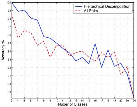
Figure 2: The performance of hierarchical multiclass decompositions and ‘all-pairs’ decompositions on 20 authorship determination problems with varying number of classes.

7 Concluding Remarks

This paper presents a new approach for hierarchical multiclass decomposition of multinomials. A similar hierarchical approach can be attempted with nonparameteric models. For instance using any nonparametric probabilistic binary discriminator one can attempt to heuristically estimate the hardness of the involved binary problems using empirical error rates and design reasonable hierarchical decompositions. However, a major difficulty in this approach is the computational burden.

When considering the main inherent deficiency of all-pairs decompositions it appears that this deficiency should disappear or at least soften when the number of classes increases. The reason is that with large number of classes, the noisy votings of irrelevant classifiers will tend to cancel out and the power of the relevant classifiers will then increase. We therefore speculate that it would be very hard to consistently beat all-pairs decompositions with very large number of classes. Nevertheless,a desirable property of a decomposition scheme is scalability, which allows for efficient handling of large number of classes (and datasets). For example, one can hypothesize useful authorship determination applications, which need to determine between thousands or even millions of authors. While balanced hierarchical decomposition will be able to scale up to these dimensions, the $O(k^{2})$ complexity of the all-pairs method would probably start to form a computational bottleneck.

References

- Antos et al., (1999) Antos et al.][1999]LowerAntosDG99 Antos, A., Devroye, L., & Gyorfi, L. (1999). Lower bounds for bayes error estimation. Pattern Analysis and Machine Intelligence, 21, 643–645.
- Burrows, (1987) Burrows][1987]Burrows87 Burrows, J. (1987). Word patterns and story shapes: The statistical analysis of narative style. Literary and Linguistic Computing, 2, 61–70.
- Cover & Thomas, (1991) Cover and Thomas][1991]CoverT91 Cover, T., & Thomas, J. (1991). Elements of information theory. John Wiley & Sons, Inc.
- Dekel & Singer, (2002) Dekel and Singer][2002]DekelS02 Dekel, O., & Singer, Y. (2002). Multiclass learning by probabilistic embedding. Neural Information Processing Systems (NIPS).
- Dietterich & Bakiri, (1995) Dietterich and Bakiri][1995]DietterichB95 Dietterich, T., & Bakiri, G. (1995). Solving multiclass learning problems via error-correcting output codes. Journal of Artificial Intelligence Research, 2, 263–286.
- El-Yaniv et al., (1997) El-Yaniv et al.][1997]ElYanivFT97 El-Yaniv, R., Fine, S., & Tishby, N. (1997). Agnostic classification of markovian sequences. Neural Information Processing Systems (NIPS).
- Friedman, (1996) Friedman][1996]Friedman96 Friedman, J. (1996). Another approach to polychotomous classification (Technical Report). Stanford University.
- Friedman & Singer, (1998) Friedman and Singer][1998]friedman99efficient Friedman, N., & Singer, Y. (1998). Efficient bayesian parameter estimation in large discrete domains.
- Fürnkranz, (2002) Fürnkranz][2002]Furnkranz02 Fürnkranz, J. (2002). Round robin classification. Journal of Machine Learning Research, 2, 721–747.
- Griths & Tenenbaum, (2002) Griths and Tenenbaum][2002]griths-using Griths, T., & Tenenbaum, J. (2002). Using vocabulary knowledge in bayesian multinomial estimation.
- Gutman, (1989) Gutman][1989]Gutman89 Gutman, M. (1989). Asymptotically optimal classification for multiple tests with empirically observed statistics. IEEE Trans. on Information Theory, 35, 401–408.
- Har-Peled et al., (2002) Har-Peled et al.][2002]HarpeledRZ02 Har-Peled, S., Roth, D., & Zimak, D. (2002). Constraint classification for multiclass classification and ranking. Neural Information Processing Systems (NIPS).
- Lehmann, (1959) Lehmann][1959]Lehmann59 Lehmann, E. (1959). Testin statistical hypotheses. John Wiley & Sons.
- Lin, (1991) Lin][1991]Lin91 Lin, J. (1991). Divergence measures based on the shannon entropy. IEEE Transactions on Information Theory, 37, 145–151.
- McAllester & Schapire, (2000) McAllester and Schapire][2000]llester00convergence McAllester, D., & Schapire, R. E. (2000). On the convergence rate of good-Turing estimators. Proc. 13th Annu. Conference on Comput. Learning Theory (pp. 1–6). Morgan Kaufmann, San Francisco.
- Mitchell, (1999) Mitchell][1999]mitchell99machine Mitchell, T. (1999). Machine learning and data mining. Communications of the ACM, 42, 30–36.
- Mosteller & Wallace, (1964) Mosteller and Wallace][1964]MostellerW64 Mosteller, F., & Wallace, D. (1964). Inference and disputed authorship: The federalist. Addison-Wesley.
- Rao & Rohatgi, (2000) Rao and Rohatgi][2000]Rao00 Rao, J., & Rohatgi, P. (2000). Can pseudonymity really guarantee privacy? USENIX Security Symposium.
- Ristad, (1998) Ristad][1998]ristad95natural Ristad, E. (1998). A natural law of succession. IEEE International Symposium on Information Theory (pp. 216–21).
- Sejnowski & Rosenberg, (1987) Sejnowski and Rosenberg][1987]SejnowskiR87 Sejnowski, T., & Rosenberg, C. (1987). Parallel networks that learn to pronounce English text. Journal of Complex Systems, 1, 145–168.
- Stamatatos et al., (2001) Stamatatos et al.][2001]StamatatosFK Stamatatos, E., Fakotakis, N., & Kokkinakis, G. (2001). Automatic text categorisation in terms of genre and author. Computational Linguistics, 26, 471–495.
- Wong & You, (1985) Wong and You][1985]WongY85 Wong, A., & You, M. (1985). Entropy and distance of random graphs with application to structural pattern recognition. Pattern Analysis and Machine Intelligence, 7, 599–609.