Dynamics of solar wind protons reflected by the Moon

Abstract

Solar system bodies that lack a significant atmosphere and significant internal magnetic fields, such as the Moon and asteroids, have been considered as passive absorbers of the solar wind. However, ion observations near the Moon by the SELENE spacecraft show that a fraction of the impacting solar wind protons are reflected by the surface of the Moon. Using new observations of the velocity spectrum of these reflected protons by the SARA experiment on-board the Chandrayaan-1 spacecraft at the Moon, we show by modeling that the reflection of solar wind protons will affect the global plasma environment. These global perturbations of the ion fluxes and the magnetic fields will depend on microscopic properties of the object’s reflecting surface. This solar wind reflection process could explain past ion observations at the Moon, and the process should occur universally at all atmosphereless non-magnetized objects.

1 Introduction

Traditionally, bodies that lack a significant atmosphere and internal magnetic fields, such as the Moon and asteroids, have been considered passive absorbers of the solar wind (Cravens, 2004). The solar wind ions and electrons directly impact the surface of these bodies due to the lack of atmosphere, and the interplanetary magnetic field passes through the obstacle relatively undisturbed because the bodies are assumed to be non-conductive. Since the solar wind is absorbed by the body, a wake is created behind the object. This wake is gradually filled by solar wind plasma downstream of the body, through thermal expansion and the resulting ambipolar electric field, along the magnetic field lines (Farrell et al., 1998), This picture of the interaction between the Moon (and asteroids) and the solar wind, is based on in-situ observations of ions, electrons, and magnetic fields by many missions (Schubert and Lichtenstein, 1974; Ogilvie et al., 1996; Halekas et al., 2005; Nishino et al., 2009b).

However, there have been observations that do not easily fit into this picture of atmosphereless bodies as the passive absorbers of the solar wind.

On the Moon, the Apollo 12 and 14 Suprathermal Ion Detector (SIDE) observed energetic ion fluxes at the nightside surface (Freeman, 1972). Also, Nozomi observed non-thermal ions at large distances from, and upstream of, the Moon (Futaana et al., 2003). Such ions are not easily explained in the traditional picture of the Moon–solar wind interaction.

Recent observations at the Moon by the SELENE (Selenological and Engineering Explorer) mission (Saito et al., 2008) and by the Chandrayaan-1 mission (Goswami and Annadurai, 2009) might provide a clue to many of these unexplained observations. Ion detectors on-board SELENE observed that some of the solar wind protons (around 0.1%) are reflected by the Lunar surface, which was unexpected, since it has been assumed that all solar wind protons are neutralized on impact with the Lunar surface (Crider and Vondrak, 2002).

Also, the ion detector (SWIM) of the SARA experiment on-board the Chandrayaan-1 mission (Bhardwaj et al., 2005; McCann et al., 2007; Barabash et al., 2009; Wieser et al., 2009) observes these reflected solar wind protons, and in Fig. 1 we show the energy spectrum of one such observation. The sunward sectors of the detector see an undisturbed solar wind, while the surface looking sectors see reflected protons with a broader energy distribution. These observations show that the simplified picture of atmosphereless bodies as passive absorbers of the solar wind is incomplete.

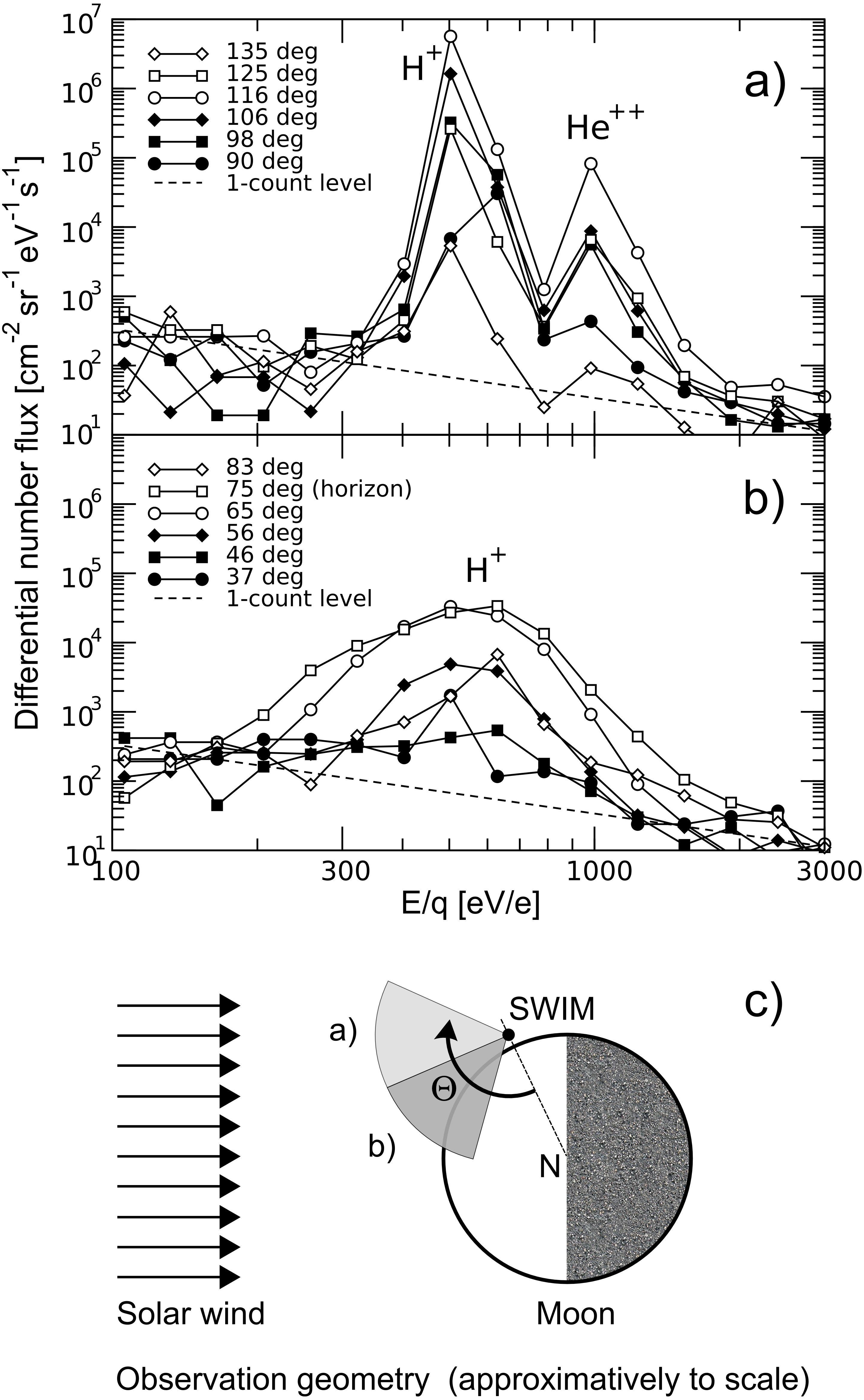
Figure 1: Ion observations on February 19, 2009, by the SWIM sensor, of the SARA instrument, on Chandrayaan-1. In (a) and (b) we show ion energy spectra from different directions, and in (c) the observation geometry is illustrated. The view directions are approximately in the equatorial plane, and they are labeled by the angle, $\Theta$, to the nadir direction. The spectra in (a) show the undisturbed solar wind from 106 and 116 deg, while the spectra in (b) show the protons reflected from the surface. The spectra are averaged over 30 minutes, and are from twelve of the 16 sectors (the remaining four sectors show only background values). The plane of the illustration in (c) is approximately the equatorial plane. Chandrayaan-1 is in a circular polar orbit at 100 km altitude (Goswami and Annadurai, 2009). The SWIM sensor has a total field of view of $7.5^{\circ}$ FWHM $\times 180^{\circ}$ divided into 16 sectors, and a time resolution of 8 seconds (McCann et al., 2007). The energy resolution is $dE/E=0.07-0.08$, depending on viewing direction.

The reflection of solar wind ions on solar system bodies that lack a significant atmosphere affects the solar wind interaction, where the microphysical properties of the reflecting surface will perturb the global ion and magnetic field environment near the object. We illustrate this effect on the solar wind interaction by modeling results for ions near the Moon. In particular, we show that this model can explain the SARA/Chandrayaan-1 ion observations (Fig. 1) and the observations of non-thermal ions by the Nozomi mission (Futaana et al., 2003).

2 Model

We present a model of the surface reflection of solar wind protons at the Moon and its effects on the global ion distribution in the vicinity of the Moon. Reflection (or back scattering) of solar wind protons on the surface of a solar system body is a process where some of the solar wind protons that impact the surface will recoil on atoms in the top atomic layers of the regolith, with only a slight reduction in velocity.

We assume that there are three basic parameters that characterize the reflection process, (1) the fraction of the precipitating protons that are reflected, $f_{r}$, i.e. the probability that a proton is reflected. We assume here that it is a constant, independent of impact velocity. (2) the speed of a reflected protons, as a fraction of the impact speed, $f_{v}$, and (3) the directional (angular) distribution of the reflected protons. The first published observation of reflected protons was by SELENE at the Moon (Saito et al., 2008). Their estimate is that the reflected fraction $f_{r}=0.001-0.01$ (this is consistent with estimates from SWIM observations), and that the velocity magnitude of the reflected protons is 80% of the solar wind velocity magnitude, $f_{v}=0.8$. Regarding the angular distribution of the reflected protons, Saito et al. (2008) find that it is much broader than that of the solar wind ions, thus the observed ions are not specularly reflected but rather scattered at the lunar surface. Since the exact angular distribution is unknown, we have used four different reflection models for determining the velocity direction of the reflected ion.

• Specular. For specular reflections, the protons’ velocity vector before and after the reflection are in the same plane, and the angle to the surface normal is the same. So, an ion inside the spherical obstacle at the position $\mathbf{r}$, with velocity $\mathbf{v}$, is reflected by updating the velocity to $\mathbf{v^{\prime}}=\mathbf{v}-2\left(\mathbf{v}\cdot\mathbf{\hat{r}}\right)\mathbf{\hat{r}}$, where $\mathbf{\hat{r}}=\mathbf{r}/|\mathbf{r}|$.

• Perpendicular, $\mathbf{v^{\prime}}$ is perpendicular to the surface of the spherical obstacle (parallel to the surface normal).

• cos²-perpendicular. The angle between $\mathbf{v^{\prime}}$ and the surface normal, $\theta$, is randomly drawn from a $\cos^{2}\theta$ probability distribution.

• cos²-specular. The angle between $\mathbf{v^{\prime}}$ and the direction of specular reflection (see above), $\theta$, is randomly drawn from a $\cos^{2}\theta$ probability distribution.

These different reflection models are illustrated in Fig. 2d. If not noted otherwise, we have used the cos²-specular reflection model since that gave the best fit to the observations.

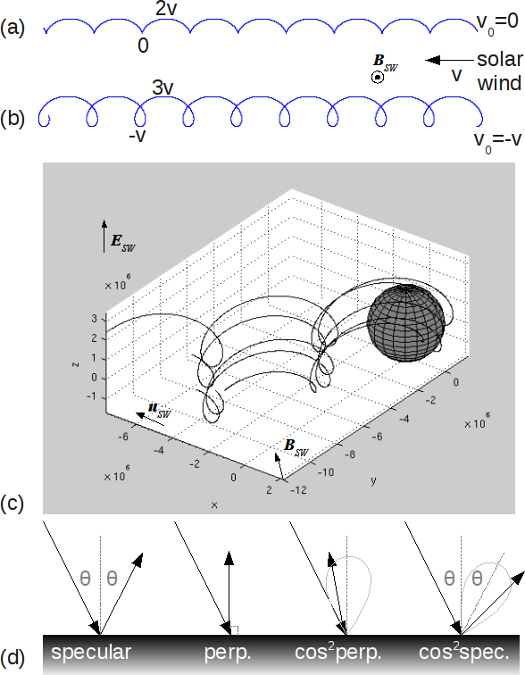
Figure 2: (a) The cycloid trajectory of a pick-up ion where the initial velocity is zero, and a solar wind of velocity $v$ is inflowing from the right. The solar wind magnetic field, $\mathbf{B}_{sw}$, is directed out of the page. The solar wind convectional electric field is $\mathbf{E}_{sw}=\mathbf{v}\times\mathbf{B}_{sw}$. The ion velocity vary between $0$ and $2v$ along the trajectory. (b) The trajectory of an ion injected into the solar wind with velocity $-v$. This is equivalent to a pick-up ion with zero velocity in a solar wind of velocity $2v$, as seen by an observer moving with velocity $-v$. In the frame of the illustration, where the plasma flow to the left with velocity $v$, the ion velocity will vary between $-v$ and $3v$ along the trajectory. (c) Sample trajectories of protons launched perpendicular to the lunar surface. (d) Illustration of some different reflection models, i.e. different ways of selecting the direction of the velocity vector of a proton that has reflected on the planetary surface.

When a solar wind proton has reflected, it will travel in a cycloid motion, gyrating around the magnetic field lines. The motion of the ion with charge $q_{i}$ and velocity $\mathbf{v}_{i}=\mathbf{v}_{i}(t)$ is governed by the Lorentz force,

$$q_{i}\left(\mathbf{E}+\mathbf{v}_{i}\times\mathbf{B}\right)=q_{i}(\mathbf{v}_{i}-\mathbf{v}_{sw})\times\mathbf{B}_{sw}$$

since the solar wind convective electric field is $\mathbf{E}_{sw}=-\mathbf{v}_{sw}\times\mathbf{B}_{sw}$. Here $\mathbf{v}_{sw}$ and $\mathbf{B}_{sw}$ is the solar wind velocity, and the IMF, respectively. We have assumed constant solar wind conditions.

For an ion with zero initial velocity, this lead to the classical trajectory of a pick-up ion as illustrated in Fig. 2a. Since the reflected protons have non-zero velocity in a coordinate system where the reflecting body is stationary, the trajectory will be different, as shown in Fig. 2b. In addition to the cycloid motion perpendicular to the IMF, the ion will also drift with a constant velocity along the IMF, if the initial velocity of the ion had a non-zero velocity component along the IMF. The trajectories of five ions, launched perpendicular to the Lunar surface at (lng,lat) = (0,0) and (+-30,+-30) degrees with velocities of 175 km/s in a 350 km/s solar wind are shown in Fig. 2c as an illustration of this combined cycloid and drift motion. The solar wind magnetic field has a magnitude of 3 nT and is directed along $(-1,1,0)$. Since the launched protons have non-zero velocity components along the magnetic field they will travel along the field line in addition to the ideal cycloid motion shown in Fig. 2b. The coordinate system has the $x$-axis from the center of the Moon toward the Sun, the $y$-axis in the ecliptic plane, and the $z$-axis in the northern ecliptic hemisphere.

Previous investigations of ion trajectories near the Moon have considered ions produced by photoionization of exospheric neutrals (Manka and Michel, 1970, 1973), not reflected ions. Neither has previous global models of the Moon’s interaction with the solar wind included reflected solar wind protons (Kimura and Nakagawa, 2008; Trávníček et al., 2005; Kallio, 2005; Harnett and Winglee, 2003). However, in a more general setting, Shimazu (1999) saw acceleration of reflected ions in hybrid simulations of plasma flow around a generic obstacle.

For the modeling of reflected protons at the Moon we have used a test particle approach, where the trajectory of each proton is computed by integrating the Lorenz’ force for constant solar wind conditions, i.e. constant solar wind conditions throughout the simulations domain. In what follows, the coordinate system used is centered at the Moon and has its $x$-axis toward the Sun, a $z$-axis perpendicular to the ecliptic plane, in the northern hemisphere, and a $y$-axis that completes the right handed system. The outer boundary of the simulation domain is a box centered at the Moon with sides of length 8000 km. The inner boundary is a sphere of radius 1730 km. At the start of the simulation the domain is empty of particles. Before each time step we fill the $x$-axis shadow cells (cells just outside the simulation domain) with proton meta-particles with weight $N_{m}=7.5\cdot 10^{20}$ (number of real protons per meta-particle). The proton meta-particles are drawn from a Maxwellian distribution with a specified temperature and bulk velocity. After each time step the shadow cells and the obstacle region are emptied of protons. A fraction, $f_{r}$, of the protons found inside the obstacle are selected to be reflected, randomly, with a velocity magnitude that is reduced by a fraction $f_{v}$. The boundary conditions in the $y$- and $z$-directions are periodic. We have $N_{I}$ (meta-)ions at positions $\mathbf{r}_{i}(t)$ [m] with velocities $\mathbf{v}_{i}(t)$ [m/s], mass $m_{i}$ [kg] and charge $q_{i}$ [C], $i=1,\ldots,N_{I}$. Using a Leap-Frog integrator, the trajectories of the ions are computed from the Lorentz force,

$$\frac{\displaystyle d\mathbf{r}_{i}}{\displaystyle dt}=\mathbf{v}_{i},\quad\frac{\displaystyle d\mathbf{v}_{i}}{\displaystyle dt}=\frac{\displaystyle q_{i}}{\displaystyle m_{i}}\left(\mathbf{E}+\mathbf{v}_{i}\times\mathbf{B}\right),\quad i=1,\ldots,N_{I}$$

where $\mathbf{E}=\mathbf{E}(\mathbf{r},t)$ is the electric field, and $\mathbf{B}=\mathbf{B}(\mathbf{r},t)$ is the magnetic field, and time is stepped forward by 0.05 s In Fig. 3 we show results for a model run with a solar wind with a velocity of 350 km/s, a temperature of 48000 K, and a magnetic field that is $(-2.12,2.12,0)$ nT, at time 20 s (when the solution has reached a steady state). The velocity of the reflected protons is reduced by $f_{v}=0.5$. Note that this is for the case of complete reflection of all precipitating protons ($f_{r}=1$), but this can be scaled for other reflection fractions, e.g., by 1/100 for a 1% reflection.

In reality the solar wind flow is affected by the presence of the Moon and the reflected protons. To correctly model this a self-consistent model is needed, at a considerable computational cost. Also, since this is a first attempt to model the effects of reflected protons, and the details of the reflection process is not known, a fully self consistent model of the process would not add much to the investigation. To justify the use of the test particle approach we did a self-consistent hybrid model (Holmström, 2009) run using the same parameter values as used in Fig. 3.

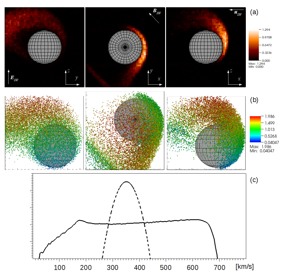
Figure 3: Results for a test particle simulation run. (a) Magnitude of the $yz$-component of the proton number flux (number density times average velocity) around the Moon, relative to the magnitude of the solar wind proton number flux. This is for the case of 100% reflection ($f_{r}=1$) of the precipitating protons, but can be scaled for any other value of $f=1$. Shown are cuts through the planes $x=0$ (left), $z=0$ (middle), and $y=0$ (right). (b) The reflected proton meta particles, colored by velocity magnitude (relative to the solar wind velocity). (c) The velocity spectrum of all protons in the simulation domain. The $x$-axis unit is km/s, and the $y$-axis scale is logarithmic in arbitrary units. The solid line is the reflected protons, and the dashed line is the solar wind protons.

The result is shown in Fig. 4.

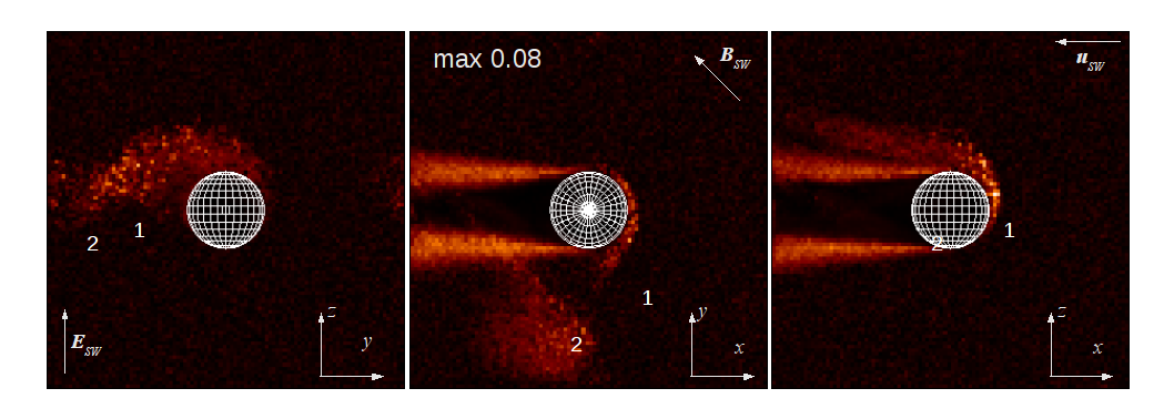
Figure 4: Solar wind proton reflection using a hybrid model. Shown is the magnitude of the $yz$-component of the proton number flux, as in Fig. 3a. The test particle run is the same as in Fig. 3. The additional parameters for the hybrid run is $\mathbf{n}_{sw}=5$ cm^-3, $\mathbf{T}_{e}=10000$ K, $\gamma=5/3$, $\Delta t=0.08$ s, five subcycles per time step, $f_{r}=0.05$, approximately 8 million meta-protons, the simulation domain is twice as large (a cube with sides 16000 km), and the grid has 100 cells along each dimension (one million cells in total). Also shown, by numbers, is the position of the two Nozomi observations that are presented in Fig. 6.

We see that the morphology of the reflected ion fluxes are similar, although the maximum flux is smaller in the test particle case (0.065 times the solar wind flux, i.e. 1.3 times the reflection of 0.05 used in the hybrid model) compared to the hybrid model (0.08), probably due to statistical fluctuations in the hybrid simulation. In the hybrid simulation we also see the wake refill behind the Moon, which is not present in the test particle simulation, but that is acceptable, since we are mostly interested in the dayside dynamics of the reflected solar wind protons.

3 Model Results and Comparison with Observations

We now investigate in more detail the general morphology of the reflected ions. The proton flux, in directions perpendicular to the solar wind flow direction, around the Moon is shown in Fig. 3a. The global effects of the reflected protons are clearly visible. The reflected solar wind protons create a plume of ions that initially are accelerated along the solar wind electric field direction, then drift along the IMF direction, and gyrate perpendicular to the IMF. The density of reflected ions is highest near the sub solar point, then decrease tailward from dispersion due to different initial velocities. At the cusps of the cycloid motion there is however a density increase, as seen in the lower left corner of the middle plot of Fig. 3a. The maximum density is 1.3 times the solar wind density when all protons are reflected. So if 1% of the solar wind protons are reflected the maximum density would be 0.013 times the solar wind density.

In Fig. 3b is shown the meta-particles that correspond to the reflected ions. The cycloid motion, and acceleration along $\mathbf{E}_{sw}$ is again clearly visible. The velocity spectrum of all protons in the simulation domain in Fig. 3c, shows the solar wind population, and the much broader distribution of reflected ions. This broadening of the spectrum is consistent with the broadening of the observed spectrum for look direction toward the lunar surface, as shown in Fig. 1b. The similarity between the observed and modeled spectrum is even better if we only include protons in the model that are close to the position of Chandrayaan-1 at the observation time. In Fig. 5 we show the spectra of reflected protons in three latitude bands, with Fig. 5b corresponding closest to the observation position in the ecliptic plane. Only protons with velocities away from the Moon are included, to approximate the SWIM view conditions. The observed spreading of the solar wind spectrum to lower and higher energies is seen in the model spectrum. That the peak of the model spectrum is so much lower in energy than the solar wind (not seen in the observed spectrum), might indicate that the model reduction in velocity ($f_{v}=0.5$) is too large. This is consistent with the SELENE observation that $f_{v}=0.8$ (Saito et al., 2008).

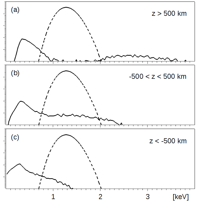
Figure 5: Energy spectra of reflected protons (solid lines) and solar wind protons (dashed lines). Corresponding to the spectrum in Fig. 3c, but instead of including all protons in the domain, each spectrum is for selected regions of the simulation domain. The included protons are those on the dayside ($x>0$) at altitudes less than 200 km with $z$ coordinates in the ranges (a) $z>500$ km, (b) -500 $<z<500$ km, and (c) $z<-500$ km. The solid line is the reflected protons, and the dashed line is the solar wind protons. The $y$-axes are logarithmic in arbitrary units.

We now use the test particle model to also investigate if reflected protons can explain the observations of non-thermal ions by the Nozomi mission. In Futaana et al. (2003), Fig. 5, ion velocity spectra taken at two different times during the Nozomi Lunar flyby are presented. To compare the results of the test particle model with Nozomi’s ion observation, we must first of all select appropriate solar wind conditions. The estimated solar wind conditions in (Futaana et al., 2003) is 350 km/s with an IMF of magnitude 3 nT, $(-2.12,2.12,0)$ nT. However, there are uncertainties in this IMF estimate since the direction was obtained from the observed temperature anisotropy in the electron velocity spectrum, and Futaana et al. (2003) estimate the uncertainty in IMF direction to 20^∘. Due to this uncertainty, and since the trajectories of reflected protons are sensitive to the IMF, we tried different IMFs and found a best fit for $(-2.82,1.03,0)$ nT, i.e. about 25^∘away from the estimate by Futaana et al. (2003). In Fig. 6 we compare velocity space plots of the test particle model with Nozomi’s ion observation (Fig. 5 in Futaana et al. (2003)).

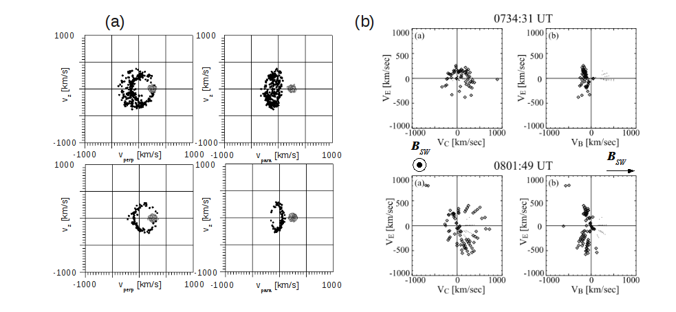
Figure 6: The reflected protons in velocity space. Comparison of (a) test particle model at time 120 s, with (b) Nozomi observations. Top row is the velocity space distribution projected along $\mathbf{B}_{sw}$ (left) and perpendicular to $\mathbf{B}_{sw}$ (right). Shown are all simulation meta-particles in a cube with side of 500 km, centered at the positions of the observations, (2500,-3700,-900) km and (-600,-5500,-1400) km, respectively. These positions are shown in Fig. 4. In gray are the solar wind protons, and in black are the reflected protons. The plots in (b) are from Futaana et al. (2003, Fig. 5). The solar wind conditions used in the simulation has a velocity of 350 km/s, a temperature of 48000 K, and a magnetic field that is $(-2.82,1.03,0)$ nT. The reflection model is cos² specular.

We see clear similarities in the observed and modeled velocity space distributions. This shows that reflected protons is a possible explanation for the observed nonthermal ions. The discrepancies in distributions could be due to a change in the IMF between the two observation times. For an illustration of the observation geometry, see Fig. 2 in (Futaana et al., 2003). This show that the Nozomi ion observations, even upstream of the moon, can be explained by reflected solar wind ions.

To illustrate the global effects of different assumptions for the local reflection process, Fig. 7 show the effect of perpendicular reflection, and of no velocity loss at reflection, $f_{v}=1$. The perpendicular reflection model give less velocity dispersion of the reflected ions, and lead to more than three times the solar wind number flux (assuming all protons are reflected). No velocity loss at reflection on the other hand lead to a larger velocity dispersion, and a more diffuse plume of ions, with only 0.7 times the solar wind flux.

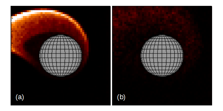
Figure 7: Different reflection processes. Here it is illustrated how the global solar wind interaction is perturbed by changes in the local microphysics of the reflection process. Shown is the magnitude of the $yz$-component of the proton number flux, relative to the magnitude of the solar wind proton flux, in the plane $x=0$, when the reflected protons are (a) perpendicular to the lunar surface with $f_{v}=0.5$, and (b) reflected according to the cos²-specular model, without losing velocity ($f_{v}=1$). The different reflection processes are illustrated in Fig. 2d and the color scale is the same as in Fig. 3a. All other parameters for these two simulation runs are the same as for that in Fig. 3.

To illustrate the sensitivity of the reflected protons to the microphysics of the reflection process, we show in Fig. 8 how the velocity space distributions of the reflected protons change when we assume a cos² perpendicular and a specular reflection model.

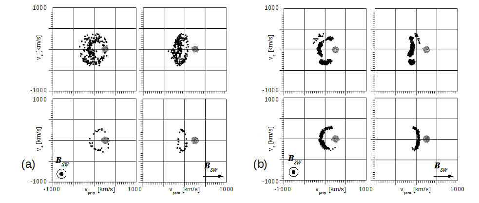
Figure 8: The reflected protons in velocity space from the test particle model for the same Nozomi comparison as shown in Fig. 6. This is a comparison of two different reflection models. (a) cos² perpendicular, and (b) specular. Both cases has the same solar wind conditions as in Fig. 6.

4 Discussion

We can compare the surface reflected ions with pick-up ions, observed at comets, Mars and Venus. In a frame following the reflected ions, the situation is similar. So a reflected proton behaves as a pick-up ions seeing a faster solar wind (from different directions for all reflected ions). This will create a ring distribution in velocity space, as was observed at the Moon (Futaana et al., 2003). The cycloid trajectory of these reflected ions can take them deep into the wake of the Moon, which has been observed by SELENE (Nishino et al., 2009a), giving a possible explanation for the Apollo observations of solar wind energy ions at the night side surface of the Moon (Freeman, 1972). These were bursts of ions in the keV range, with fluxes of the order 10⁶ cm^-2 s^-1 sr^-1, and mass per unit charge less than 10 amu/q, and hence thought to be of solar wind origin.

It is interesting to note that a local process (surface reflection) can perturb the global interaction of the Moon with the solar wind. Also, the character of this global interaction depends on the details of the local process, e.g., the velocity distribution of the reflected protons. Thus, it is possible to infer properties of the local reflection process from far away observations of the ion distributions.

If we consider the energies involved in the reflection process, the kinetic energy density of the reflected ions is $W_{r}=f_{r}{n}_{sw}m_{p}(f_{v}{v}_{sw})^{2}/2$ where $m_{p}$ is the proton mass, and the magnetic field energy density is $W_{B}={B}_{sw}^{2}/(2\mu_{0})$ where $\mu_{0}$ is the magnetic constant. Using $f_{r}=0.01$, $n_{sw}=5$ cm^-3, $f_{v}=0.5$, $v_{sw}=350$ km/s, and $B_{sw}$ = 3 nT, we get that $W_{r}/W_{B}$ = 0.35. Thus, the kinetic energy density of the reflected ions is a significant fraction of the solar wind magnetic field energy density, and the reflected ions should be a strong source of wave activity.

We can compare these reflected protons with the protons reflected by Earth’s bow shock. There, in Earth’s foreshock region, these ion beams propagate upstream in the solar wind. It is a classical case of an electromagnetic counter-streaming beam situation, with the beam density around 1% of the solar wind density. This causes wave activity, and has been studied for a long time in great detail, see e.g. Tsurutani and Rodriguez (1981).

The reflection of solar wind ions should be a universal process that occur at all bodies without a significant atmosphere, e.g., at asteroids, and at the Martian moons Phobos and Deimos.

References

- Barabash et al. (2009) Stas Barabash et al. Investigation of the solar wind–Moon interaction onboard Chandrayaan-1 mission with the SARA experiment. Current Science, 96(4):526–532, 2009.
- Bhardwaj et al. (2005) A. Bhardwaj, S. Barabash, Y. Futaana, Y. Kazama, K. Asamura, D. McCann, R. Sridharan, M. Holmstrom, P. Wurz, and R. Lundin. Low energy neutral atom imaging on the Moon with the SARA instrument aboard Chandrayaan-1 mission. Journal of Earth System Science, 114:749–760, December 2005. doi: 10.1007/BF02715960.
- Cravens (2004) Thomas E. Cravens. Physics of Solar System Plasmas. Cambridge University Press, 2004.
- Crider and Vondrak (2002) D. H. Crider and R. R. Vondrak. Hydrogen migration to the lunar poles by solar wind bombardment of the moon. Advances in Space Research, 30(8):1869–1874, 2002.
- Farrell et al. (1998) W. M. Farrell, M. L. Kaiser, J. T. Steinberg, and S. D. Bale. A simple simulation of a plasma void: Applications to Wind observations of the lunar wake. Journal of Geophysical Research, 103:23653–23660, 1998. doi: 10.1029/97JA03717.
- Freeman (1972) J. W. Freeman, Jr. Energetic ion bursts on the nightside of the moon. Journal of Geophysical Research, 77:239–243, 1972. doi: 10.1029/JA077i001p00239.
- Futaana et al. (2003) Y. Futaana, S. Machida, Y. Saito, A. Matsuoka, and H. Hayakawa. Moon-related nonthermal ions observed by Nozomi: Species, sources, and generation mechanisms. Journal of Geophysical Research (Space Physics), 108:1025, 2003. doi: 10.1029/2002JA009366.
- Goswami and Annadurai (2009) J.N. Goswami and M. Annadurai. Chandrayaan-1: India’s first planetary science mission to the moon. Current Science, 96(4):486–491, 2009.
- Halekas et al. (2005) J. S. Halekas, S. D. Bale, D. L. Mitchell, and R. P. Lin. Electrons and magnetic fields in the lunar plasma wake. Journal of Geophysical Research (Space Physics), 110(A9):7222, 2005. doi: 10.1029/2004JA010991.
- Harnett and Winglee (2003) E. M. Harnett and R. M. Winglee. 2.5-D fluid simulations of the solar wind interacting with multiple dipoles on the surface of the Moon. Journal of Geophysical Research (Space Physics), 108:1088, 2003. doi: 10.1029/2002JA009617.
- Holmström (2009) M. Holmström. Hybrid modeling of plasmas. To appear in the Proceedings of the 8th European Conference: Numerical Mathematics and Advanced Applications, Springer. http://arxiv.org/abs/0911.4435, 2009.
- Kallio (2005) E. Kallio. Formation of the lunar wake in quasi-neutral hybrid model. Geophysical Research Letters, 32:L06107, 2005.
- Kimura and Nakagawa (2008) Shinya Kimura and Tomoko Nakagawa. Electromagnetic full particle simulation of the electric field structure around the moon and the lunar wake. Earth Planets Space, 60:591–599, 2008.
- Manka and Michel (1970) R. H. Manka and F. C. Michel. Lunar Atmosphere as a Source of Argon-40 and Other Lunar Surface Elements. Science, 169:278–280, July 1970.
- Manka and Michel (1973) R. H. Manka and F. C. Michel. Lunar ion energy spectra and surface potential. In Lunar and Planetary Science Conference, volume 4 of Lunar and Planetary Science Conference, pages 2897–2908, 1973.
- McCann et al. (2007) D. McCann, S. Barabash, H. Nilsson, and A. Bhardwaj. Miniature ion mass analyzer. Planetary and Space Science, 55:1190–1196, June 2007. doi: 10.1016/j.pss.2006.11.020.
- Nishino et al. (2009a) M. N. Nishino, M. Fujimoto, K. Maezawa, Y. Saito, S. Yokota, K. Asamura, T. Tanaka, H. Tsunakawa, M. Matsushima, F. Takahashi, T. Terasawa, H. Shibuya, and H. Shimizu. Solar-wind proton access deep into the near-Moon wake. Geophysical Research Letters, 36:16103, August 2009a. doi: 10.1029/2009GL039444.
- Nishino et al. (2009b) M. N. Nishino, K. Maezawa, M. Fujimoto, Y. Saito, S. Yokota, K. Asamura, T. Tanaka, H. Tsunakawa, M. Matsushima, F. Takahashi, T. Terasawa, H. Shibuya, and H. Shimizu. Pairwise energy gain-loss feature of solar wind protons in the near-Moon wake. Geophysical Research Letters, 36:12108, June 2009b. doi: 10.1029/2009GL039049.
- Ogilvie et al. (1996) K. W. Ogilvie, J. T. Steinberg, R. J. Fitzenreiter, C. J. Owen, A. J. Lazarus, W. M. Farrell, and R. B. Torbert. Observations of the lunar plasma wake from the WIND spacecraft on December 27, 1994. Geophysical Research Letters, 23:1255–1258, 1996. doi: 10.1029/96GL01069.
- Saito et al. (2008) Y. Saito, S. Yokota, T. Tanaka, K. Asamura, M. N. Nishino, M. Fujimoto, H. Tsunakawa, H. Shibuya, M. Matsushima, H. Shimizu, F. Takahashi, T. Mukai, and T. Terasawa. Solar wind proton reflection at the lunar surface: Low energy ion measurement by MAP-PACE onboard SELENE (KAGUYA). Geophysical Research Letters, 35:L24205, 2008.
- Schubert and Lichtenstein (1974) G. Schubert and B. R. Lichtenstein. Observations of moon-plasma interactions by orbital and surface experiments. Reviews of Geophysics and Space Physics, 12:592–626, November 1974.
- Shimazu (1999) H. Shimazu. Three-dimensional hybrid simulation of magnetized plasma flow around an obstacle. Earth, Planets, and Space, 51:383–393, 1999.
- Trávníček et al. (2005) P. Trávníček, P. Hellinger, D. Schriver, and S. D. Bale. Structure of the lunar wake: Two-dimensional global hybrid simulations. Geophysical Research Letters, 32:L06102, 2005.
- Tsurutani and Rodriguez (1981) B. T. Tsurutani and P. Rodriguez. Upstream waves and particles - An overview of ISEE results. Journal of Geophysical Research, 86:4319–4324, 1981. doi: 10.1029/JA086iA06p04317.
- Wieser et al. (2009) Martin Wieser, Stas Barabash, Yoshifumi Futaana, Mats Holmström, Anil Bhardwaj, R. Sridharan, M.B. Dhanya, Peter Wurz, Audrey Schaufelberger, and Kazushi Asamura. Extremely high reflection of solar wind protons as neutral hydrogen atoms from regolith in space. Planetary and Space Science, 57(14-15):2132–2134, 2009.