[O III] Equivalent Width and Orientation Effects in Quasars
Abstract
The flux of the [OIII] 5007Å line is considered to be a good indicator of the bolometric emission of quasars. The observed continuum emission from the accretion disc should instead be strongly dependent on the inclination angle between the disc axis and the line of sight. Based on this, the equivalent width (EW) of should provide a direct measure of . Here we analyze the distribution of EW([OIII]) in a sample of 6,000 SDSS quasars, and find that it can be accurately reproduced assuming a relatively small intrinsic scatter and a random distribution of inclination angles. This result has several implications: 1) it is a direct proof of the disc-like emission of the optical continuum of quasars; 2) the value of EW([OIII]) can be used as a proxy of the inclination, to correct the measured continuum emission and then estimate the bolometric luminosity of quasars; 3) the presence of almost edge-on discs among broad line quasars implies that the accretion disc is not aligned with the circumnuclear absorber, and/or that the covering fraction of the latter is rather small. Finally, we show that a similar analysis of EW distributions of broad lines (H, Mg II, C IV) provides no evidence of inclination effects, suggesting a disc-like geometry of the broad emission line region.
keywords:
Galaxies: active1 Introduction
The primary optical/UV emission of quasars is thought to arise from an accretion disc surrounding a supermassive black hole. Radiatively efficient discs (as expected in quasars, Marconi et al. 2004, and described by the Shakura & Sunyaev 1972 model), are geometrically thin and optically thick. Therefore, their observed emission should scale with the cosine of the disc inclination angle with respect to the line of sight. This is a basic element of any model of quasar emission, yet it is rather difficult to test directly, given the uncertainties on the measurements of the intrinsic continuum emission.
The obvious way to perform a check of the disc geometry of the optical/UV emitter is through a comparison with an inclination-independent indicator of the intrinsic quasar luminosity.
Such an indicator should have: 1) a negligible contamination from processes other than AGN emission (such as nuclear star formation), and 2) a small scatter in its functional dependence from the bolometric luminosity.
The first requirement is matched by several observables, for instance the hard X-ray flux, the flux of broad emission lines, and that of high-ionization narrow emission lines, such as [OIII] 5007 Å (Mulchaey et al. 1994), [OIV] 24.5 m (Rigby et al. 2009). The second requirement is hard to quantify, due to the lack of independent ways to measure the intrinsic bolometric emission. Therefore, the calibration of these indicators is not an absolute one, and is instead based on internal consistency.
In this paper we propose an easy and direct way to (a) calibrate the [OIII] flux as an indicator of the intrinsic luminosity, and (b) to estimate the inclination effects on the continuum emission of quasars, based on the analysis of the distribution of the [OIII] equivalent width (EW) in the Sloan Digital Sky Survey (SDSS) DR5 quasar sample (Schneider et al. 2007).
2 General method and sample selection
The starting point of our analysis is the following, straightforward consideration, valid for an ”idealized” quasar sample: if the [OIII] luminosity is a ”perfect” indicator of the intrinsic luminosity, and the continuum emission is due to an optically thick disc, then the distribution of [OIII] equivalent widths (EW) observed in a non-biased sample of quasars should simply reflect the distribution of disc orientations (this further assumes a negligible spread in the quasar spectral energy distribution (SED), so that the continuum luminosity at the line energy is also perfectly correlated with the total luminosity). In particular, if is the angle between the disc axis and the line of sight, we have EWO=EW, where EWO is the observed equivalent width, and EW∗ is the equivalent width as measured in a face-on disc, which in this idealized case is a fixed value for all quasars. For a population of randomly oriented discs, we expect the same number of objects per element of solid angle, and, being =EW∗/EWO, the observed distribution of [OIII] equivalent widths should be (Netzer 1985, 1990):
| (1) |
Next we estimate
how the expected distribution changes if one moves from the idealized case
described above to the ”real world”. Two main points must be considered:
the possible intrinsic spread of the [OIII]–bolometric emission relation, and
the selection effects inherent to the given sample.
1. Intrinsic spread of the [OIII]–bolometric luminosity relation.
Our working hypothesis is that on average the [OIII] luminosity is indeed a good indicator of
the bolometric luminosity. This is supported by several observational studies, where
the [OIII] flux is compared with the optical and X-ray emission (e.g. Mulchaey et al. 1994, Heckman
et al. 2005),
and by studies of the SDSS sample, where it is found that the [OIII] line is dominated by the
AGN contribution, with no significant contribution by the host galaxy, even in cases
of strong star formation activity (Kauffmann et al. 2003).
However, the spread between the emission in [OIII] and in other bands is large
(Heckman et a. 2005). This is expected, since the flux in a narrow line depends
on several variable parameters, including
the intensity and shape of the ionizing continuum, and the geometry, distance
and covering factor of the narrow line region (e.g., Baskin & Laor 2005).
A realistic description of the expected distribution of EW([OIII]) must therefore allow
for some intrinsic spread. We modeled this distribution as a Gaussian, to be convolved with the
effect of inclination described above. The goodness of the fit to the observed
distribution, and the ratio between the distribution width and the fiducial value EW0 will
assess the goodness of our hypothesis, and, in particular, of the accuracy of
the [OIII] luminosity as a proxy of the total quasar luminosity.
2. Selection effects. The sample used for our analysis is the SDSS DR5 Quasar
catalog (Schneider et al. 2007), as analyzed by Shen et al. (2008)111We have verified that the results presented in this paper
are globally unchanged if we use the new, updated catalogue by Shen et al. (2010)
recently appeared in the literature. However, this update will be included in a forthcoming
paper where we will analyze other consequences of the findings presented here..
In order to work on a well-defined, high
quality sample, we further applied the following filters: redshift range between 0.01 and 0.8,
in order to have the [OIII] line fully inside the spectral range of optimal response;
magnitude mi19.1, absolute magnitude Mi22.1 (these two criteria define a
homogeneous, well selected subsample, consisting of more than half the total DR5 quasar
sample, Richards et al. 2006); signal-to-noise per pixel higher than 5, in order to have
high quality, reliable spectra. These criteria define a sample of 6,000 quasars,
which still allows a detailed analysis of the EW([OIII]) distribution.
The main issue relevant for our work is that the flux/luminosity limit has a strong influence
on the observed EW([OIII]) distribution. Qualitatively, we expect that for a given on-axis
flux/luminosity, there will be a maximum inclination angle, above which the object will
fall below one of the two limits. Therefore, the highest inclinations
are possible only in objects with on-axis flux/luminosity much above the sample limit. These objects
are obviously expected to be rare, due to the steepness of the quasar luminosity function.
In the following Section we quantitatively discuss these points, both analytically and through a Monte-Carlo simulation. We will show that both methods clearly demonstrate that the expected slope of the distribution for high EWs is no longer dN/d(EWO)EW, as in the non-biased case described above, but dN/d(EWO)EW.
3 Data Analysis
The expected shape of the EW([OIII]) distribution can be predicted through an analytic calculation, or through numerical simulations based on the observed data themselves.
Analytic calculation. In the following, we use EW to refer to the [OIII] equivalent width, the subscript for observed quantities, and for quantities, as would be measured in sources with a face-on disc. The observed luminosity LO is given by LO=LI, and the observed equivalent width EWO=L([OIII])/LO=EW.
The differential number of objects dN with an intrinsic luminosity LI, a ”face on” equivalent width EWI, a disc inclination angle , and a distance R, is:
| (2) |
where is the intrinsic luminosity function and the distribution of the intrinsic equivalent width. We now want to transform this expression into a function of observed quantities, through the variable change (, R)(EWO, F), where F is the observed flux. Given the Jacobian of the coordinate transformation, after straightforward algebra, we obtain:
| (3) |
If the luminosity function has the form , we can rearrange the above equation and obtain the observed EW distribution as:
| (4) | |||||
We have left as the integration variable instead of , even if the luminosity selection applies to the latter quantity. The reason is the relatively flat slope below the break in the luminosity function: the integral on is essentially dominated by the upper integration limit, which is the intrinsic break luminosity and applies to . Above the break luminosity, the luminosity function is very steep; also, the integral on EWI becomes independent of the upper limit EWO when the latter is much larger than a typical EWI. We thus obtain that at the high EWO tail the observed distribution has a power law shape
| (5) |
Numerical estimate. We now reproduce the same result through a simulation,
in order to have an independent check, and to test the effects of possible deviations
of the intrinsic continuum luminosity function from the power law shape assumed above.
The simulation consists of the following steps:
1) We assume that our quasars have an
intrinsic Gaussian distribution of [OIII] equivalent width;
we further assume that the flux/luminosity distribution of our sample has the same shape
it would have if one could use the intrinsic flux/luminosity instead of the observed
ones (i.e., at any observed flux/luminosity the sample is dominated by face-on
objects).
2) We extract a random object in our sample, and measure the observed continuum
luminosity LO at the line energy.
3) We select a random disc orientation, , and derive a fictitious doubly-observed continuum luminosity LF=L,
and the analogous EWF=EW (thus ignoring the actually measured value EWO).
4) We apply an arbitrary rejection limit in terms of doubly-observed continuum flux and
luminosity, analogous to the one applied to the original sample.
5) We repeat the procedure for a large (106) number of times, and
analyze the distribution of EWF.
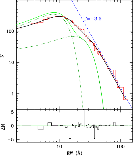
The result of this exercise is a distribution with a high-EW tail dN/dEWEWΓ, with =-3.500.01. We stress again that here we assume an intrinsic luminosity function with the same shape as the observed one. This is fully justified, since it is straightforward to show that starting from a population with a given intrinsic luminosity function, and assuming a random correction, the shape of the observed luminosity function remains unchanged. This has been also checked with our doubly observed data.
3.1 A global fit to the EW distribution
The main result of the above analysis is that, if we assume an isotropic emission of [OIII], proportional to the intrinsic disc luminosity, and a random inclination of the disc with respect to the line of sight, the observed distribution of EW([OIII]) in a flux-limited sample has a power-law tail towards high EWs with slope -3.5.
A simple look at Fig. 1 shows that such a tail is indeed present. This is our main result, to be discussed in the next Section. Here we complete the analysis looking for a global fit to the observed distribution, which is equivalent to finding the intrinsic distribution g(EWI).
Parameter Model 1 Model 2 Model 3 EW∗(Å) 7.90.4 7.10.3 8.00.3 (Å) 8.51 4.70.2 40.3 EW(Å) – – 171 (Å) – 91 110.8 – – 0.670.01 /d.o.f. 193/60 126/59 46/57
We fitted the observed distribution by convolving g(EWI) with the kernel describing the orientation effects, Equation 3, and assuming for g(EWI) various modifications of Gaussian functions. In particular, we tried three different intrinsic distributions: a single symmetric Gaussian; an asymmetric Gaussian, with two different widths for values higher and lower than the average, respectively; and two symmetric Gaussians. The first model has two free parameters in addition to a global normalization (the average EWI and the standard deviation ); the second model has three parameters (EW∗ and the left and right standard deviations, and ); the third model has five parameters (EW, , EW, , and , the relative weight of the two distributions). In fitting the observed distribution, we used a minimization technique, assuming an error equal to the square root of the number counts. The width of each bin of the distribution is 1 Å, smaller by a factor 2-3 than the typical error on single EW measurements, but large enough to have more than 15 counts in most bins, so that the use of Gaussian statistics is justified. The few bins with fewer counts have been rebinned in order to have at least 15 counts in each bin of the fitted distribution. The results of the fits clearly favour the two-Gaussian model (Table 1). The main differences between the fits are in the EW range around the distribution maximum, where a double slope change (characteristic of the two-Gaussian fit) is needed to reproduce properly the observed distribution (Fig. 1). Instead, the high-EW tail is always well fitted by a =-3.5 slope, and does not depend on the details of the intrinsic distribution. This is clear from a visual inspection of Fig. 1, where it is shown that the intrinsic distribution has an exponential drop at EW20-30 Å, and the tail at higher EW is entirely due to projection effects. This effect is even stronger for the single-peaked models, which have a narrower intrinsic distribution (Table 1). Summarizing, the results of the global fit demonstrate that: (1) an intrinsic distribution of EW([OIII]), declining exponentially at high EWs, cannot reproduce the observed distribution, due to a prominent high-EW power law tail; (2) the tail of the distribution is completely explained by disc projection effects, independently of the detailed shape of the intrinsic distribution; (3) statistically, an intrinsic distribution made up of two populations different in terms of [OIII] emission seems favoured with respect to single-peaked distributions.
The size of the sample (6,029 objects) allows an analysis of possible trends in the intrinsic distribution with other physical parameters, in particular, the continuum luminosity. We divided the sample in three parts of equal number of objects, according to their oberved continuum luminosity, and repeated the complete analysis of the EW([OIII]) distribution. In each case we obtained results fully compatible with those from the global fit, with each individual parameter consistent with the values in Table 1 at a 90% confidence level. We conclude that there is no evidence of a dependence of the results of our analysis on the observed luminosity of the sample.
3.2 The distribution of broad lines EWs
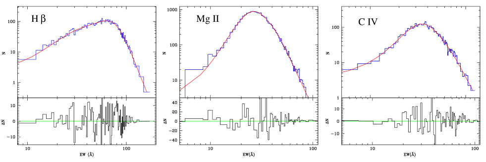
We repeated the analysis for the distributions of the equivalent widths of the main broad emission lines available in the SDSS DR5 sample, i.e. H, Mg II, and C IV. The choice of these three lines is based on the availability of high-quality fits for a large sample of quasars (Shen et al. 2008). Moreover, they cover a large range in redshift (from z=0.01 to z=4.5) and luminosity, and a span a large range of ionization (from 7.6 eV for Mg II to 13.6 eV for H, to 48 eV for C IV), possibly probing different zones of the broad line region. The samples selection criteria are the same as for the [OIII] sample, with the only difference of the redshift range for the Mg II (0.45z2.2) and the C IV (1.7z4.5) line. The three samples consist of 6,029 (H, the same as [OIII]), 19020 (Mg II) and 4468 (C IV) objects. The main results of the global fits (Fig. 2) are the following.
- In all cases, an intrinsic distribution consisting of two Gaussians provide an excellent fit (/d.o.f.1), while single Gaussian distributions, either symmetric or asymmetric, are not statistically acceptable.
- For all the three EW distributions, the intrinsic distributions fall short of fitting the high-EW
tail.
However, a power law with slope , as expected from disc projection effects
and a fully isotropic line emission, does not reproduce the
data either. A good fit can be obtained either with a steeper slope (Tab. 2)
or, alternatively assuming a fixed =-3.5, and a maximum inclination angle (cos 0.20.03)
above which the disc is no longer visible (as one would expect
if a thick torus is co-axial with the disc).
The above results clearly show that, regardless of the details of the intrinsic EW distributions, the observed EW distributions of the broad emission lines do not appear strongly affected by differential projection effects between lines and continuum.
4 Discussion
We have shown that the distribution of EW([OIII]) in SDSS quasars is a strong, direct observational proof of the disc-like structure of the continuum emission source. Furthermore, we have shown that a similar result does not hold for the main broad emission lines (H, Mg II, C IV). In the following we discuss these findings in more detail.
4.1 The distribution of EW([OIII])
The results obtained on the distribution of EW([OIII]) are interesting under several respects. The central point stressed above is the direct observational evidence of disc inclination effects. In addition to this main point, we can gain important insights on the structure of inner region of quasars.
Absence of a torus aligned with the disc. One somewhat surprising result is the absence of a maximum angle of disc inclination in our quasar sample. If we assume an optically thick torus, co-aligned with the accretion disc, and not affecting the narrow-line region (i.e. the standard assumptions of the AGN unified model), we would expect a maximum inclination angle, above which the disc become invisible. In terms of the observed distribution, this would produce a sudden decline above some EWMAX, depending on the average torus opening angle (cos EW∗/EWMAX). Instead, no deviation from is observed, which implies an upper limit on the maximum inclination angle cos 0.06. So, either (1) the torus is randomly aligned with respect to the disc, or (2) the torus covering factor is extremely small in quasars.
Parameter H Mg II C IV EW(Å) 313 23.10.3 301 (Å) 111 5.00.2 81 EW(Å) 582 291 363 (Å) 151 8.40.4 163 0.200.07 0.630.07 0.620.17 -8.00.5 -6.20.2 -5.00.4 /d.o.f. 89/97 78/67 61/72
Effects of ”limb darkening”. We can predict the modifications to the observed EW([OIII]) due to possible limb darkening effects. If we parametrize the limb darkening with a parameter , so that the observed disc luminosity scales with the inclination angle as L()(, we obtain from the calculation in Section 3 that the slope of the high-EW tail should change from to /(1+). This deviation is not observed, putting an upper limit of 0.1 at a 90% confidence limit.
Intrinsic distribution of EW([OIII]). The deconvolution of the projection effects and the determination of the intrinsic distribution of EW([OIII]) provides for the first time a quantitative estimate of the goodness of [OIII] as a proxy of the total AGN emission.
If we refer to the best fit with a single distribution (Model 2 in Table 1), the standard deviation is of the order of 50% EW∗. Such a relatively large spread is expected, given the many parameters involved in the [OIII]-total luminosity relation. In particular, two aspects are relevant: (1) the covering factor and optical depth of the narrow-line clouds, and (2) the spread in the intrinsic quasar spectral energy distribution (Elvis et al. 1994). In principle, a dependence on the intrinsic SED can be assessed in our sample: since the continuum radiation ionizing the [OIII] is in the UV range, the ratio between the [OIII] flux and the continuum at 5,000 Å should be positively correlated with the UV/optical ratio. We investigated this possibility by plotting EW([OIII]) versus the (-) and (-) SDSS colours, and found no correlation. This suggests that the first point above (the size and composition of the narrow-line clouds) dominates the intrinsic spread of EW([OIII]).
However, our best fit suggests the presence of two different populations in terms of [OIII] emission. If the two-population interpretation is correct, the calibration of the [OIII] luminosity as an indicator of the total luminosity is more complex, and subject to higher uncertainties. Moreover, in this case other differences between the two populations should be found in a more complete investigation of the spectral properties of this sample. This is obviously an important issue, which will be treated in detail in a forthcoming work. Here we only note two straightforward points: (1) the exact nature of the intrinsic distribution does not affect the main result of the power-law shape of the high-EW tail (see Section 4.2 for further details on this issue); (2) since there is no indication of a second population in the EW distributions of broad lines, the possible dichotomy observed in the [OIII] EW distribution should be due to differences in the narrow-line region properties, rather than the disc properties.
Effects on the relation between optical and X-ray emission. The hard X-ray emission of quasars is itself believed to be isotropic. Therefore, it can be used as an indicator of the bolometric luminosity, and is well known to correlate with the [OIII] emission (Heckman et al. 2005). The relation between bolometric and X-ray luminosity is complicated by the observed dependence of the optical/UV to X-ray ratio on the UV luminosity. The disc inclination obviously affects these correlations, adding a spread due to the projection effect on the UV continuum. In particular, objects which are seen nearly edge-on should have a higher (on average) X-ray to UV ratio. We note that overall we do not expect this to be a large contribution to the observed dispersion in the X-ray to UV ratio. The latter (Young et al. 2010) is of the order of a factor 3. Considering that the observed cos distribution in our sample (and in any flux-limited sample, as shown in our calculation in Section 3) is N(cos ), we expect an average value of cos =5/8, and a dispersion (defined as the interval containing 68% of the objects) of about 0.15, i.e. a factor of only . Nevertheless, in a large enough sample, a statistical correlation between the inclination angle and the observed X-ray to UV ratio should be measurable.
In order to check this, we performed the following test:
- We considered a subsample of the original 6,029 quasars, consisting of those (107) having
hard X-ray measurements. The X-ray data have been obtained from the Young et al. (2009) catalog,
made of all the SDSS DR5 quasars with serendipitous XMM-Newton observations.
- We estimated for each object the expected 2-10 keV flux, based on the
-UV luminosity correlation (Young et al. 2009).
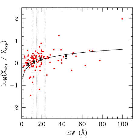
- We plotted the ratio between the expected and measured X-ray fluxes, R=FOBS/FCALC,
versus the measured EW([OIII]) for each object (Fig. 4).
- We calculated the expected R-EW relation, based on a N(cos )(cos )1.5
distribution of disc inclinations, and compared it with the observed values.
As shown in Fig. 4, even if the dispersion is large (see above), the bin-averaged R values follow the expected trend, starting below 1 at low EWs (i.e., more face-on than the average) and growing above 1 at high EWs (ie, more edge-on).
The result shown in Fig. 4 offers additional evidence in favour of our scheme. Since the presence of disc orientation effects were already proven by the analysis of the distribution of EW([OIII]), we can regard the trend in Fig. 4 as a suggestion of the hard X-ray emission being more isotropic than the optical continuum.
4.2 Uniqueness of orientation-based interpretation
The model we have discussed so far provides a reasonable interpretation of the data, but it is certainly not unique. This notwithstanding, we will argue that it is the most economic one, requiring a minimum number of ad hoc assumptions.
One possible alternative is to attribute the observed distribution of EW([OIII]) not to inclination effects, but to the intrinsic variance within the sample. A minimal variance is already included in the model (the green line in Fig. 1), but one could assume a larger one, so large as to affect the slope of the high EW tail of the distribution. However, any intrinsic distribution with a fall off steeper than a =-3.5 power law will leave unchanged the tail due to inclination effects (provided that the sample extends to high enough EW); on the other hand, an intrinsic distribution with a fall off flatter than =-3.5 will obviously produce a similarly flat tail. In conclusion, the intrinsic hypothesis would work only if (by chance) the intrinsic tail had exactly the same slope as predicted by the inclination hypothesis.
Another alternative would attribute the dimming of the observed continuum (and the enhancement of the observed EW) not to inclination, but to absorption or blocking mechanisms affecting preferentially the continuum with respect to the [OIII]. The absorption/reddening hypothesis has already been advocated in connection with some ”exceptional [OIII] emitters” (e.g. Ludwig et al. 2010); we have checked this possibility in our sample by looking for a correlation between EW and continuum colors, but have found no evidence for it. Any ad hoc escape would require a special kind of dust, a grey absorber with a frequency-independent opacity. As for the blocking variant, this has already been discussed in connection with a possible circumnuclear torus (see Section 4.1 above). In the simplest possible scheme (i.e. torus opening identical in all sources, independent of redshift and/or luminosity) we have already seen that the prediction is a sharp drop in the EW distribution, and have deduced from its non-observation a lower limit to the opening angle. If one adopts a wide distribution of opening angles, and assumes for the sake of simplicity that the cumulative effect can be described as an ”equivalent limb darkening”, then again we have found a stringent upper limit to this effect (see Section 4.1) if it were on top of the inclination; if it were in lieu of the inclination, the coincidence with the theoretical prediction (=-3.5) would again remain unexplained.
A final option could be to relax the assumption of isotropy we made for the [OIII] emission. This may happen if the [OIII] emitting clouds extend so close to the exciting nucleus as to be partly affected by the circumnuclear torus. If this were indeed the case, the EW at high inclination would be less than expected in our model, and the distribution tail would become steeper (see Section 4.3 below, where a similar scheme is discussed in connection with the EW distribution of some broad lines). One could recover the observed EW([OIII]) distribution by assuming non-isotropy for both line and continuum. Once more, we describe the angular dependence with a power law, and call and the continuum and line exponent, respectively (FOBS([OIII])(cos, FOBS(CONT)(cos).
One finds:
| (6) |
The observations require =-3.50.1 which to first order implies
| (7) |
Only a narrow strip of values in the (, ) plane are compatible with the data; of these, only our preferred choice =1, =0 has a clearcut physical justification.
It is of course possible that the actual values of and differ slightly from the “perfect disk” (=1) and “perfect [O III] isotropy” (=0) scenario.
It is also formally possible to assume for and completely different values, as long as they satisfy Eq. 7. However, such an ad-hoc assumption would not correspond to any physically plausible configuration.
4.3 The EW distribution of broad emission lines
The distributions of Fig. 3 do not show marked effects of different isotropy degrees between broad lines and continuum, at variance with the distribution of EW([OIII]). This suggests (1) a flattened structure of the broad line region, in order to have (almost) the same projection effects in both the continuum and line emission, which would cancel out in the EW, and (2) a high optical depth of the emission lines.
We can further speculate on the differences among the distributions of the three broad lines, with the EW(H) one having the steepest high-EW slope. This may be due to a somewhat rounder geometry of the line-emitting region (note however that Mg II and C IV have very different ionization levels, and in a stratified medium should bracket the location of H); or to a dependence of the emitting region geometry on the source redshift/luminosity: the redshift (and, in a flux-limited sample, the luminosity) is systematically different for the three broad-line samples considered here. In any case, the (second-order) differences among the EW distributions of the broad lines should not mask the sharp difference between all of them and EW([OIII]).
The evidence for a flattened broad line region confirms early suggestions (Netzer 1987; Collin-Souffrin & Dumont 1990; Wills & Brotherton 1995; Wanders et al. 1995; Goad & Wanders 1996) and more recent results, all based on different methods but pointing towards the same scenario:
- Spectropolarimetric observations of Seyfert 1 galaxies and quasars show distinctive features across broad emission lines which can only
be understood in terms of a rotating line-emitting disc (the BLR) surrounded by a coplanar scattering region (Smith et al. 2004, 2005).
In same cases, asymmetries in polarization spectra indicates that rotating winds are launched from these disks (Young et al. 2007).
- Maiolino et al. (2001) note an apparent paradox between the expected covering factor of BLR clouds () and the fact that the Ly-edge in absorption is never observed in quasar spectra. This paradox can be solved if the BLR is a disk and dusty gas in the outer parts, on the same plane, blocks observations along the lines of sight passing through the BLR clouds.
- McLure & Dunlop (2002) analyzed a sample of AGNs with black hole mass estimates from both reverberation mapping and stellar velocity dispersion, and showed that assuming a flattened distribution of the H emitting region provides a better match between the two estimates than a spherical shape.
- Jarvis & McLure (2006) found in a sample of radio-loud quasars a strong correlation between broad line widths and radio spectral index (considered an orientation indicator), suggesting a flattened shape of the broad line region.
- Down et al. (2010) performed a detailed analysis of H profiles in a sample of radio-loud, high-z quasars, and found that the complex observed profiles require that the line is emitted, at least in part, by a disk-like region.
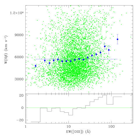
The interpretation of the observed EW distributions of broad lines as due to a flattened emission region can be tested comparing the widths of the broad lines with EW([OIII]): being EW([OIII]) an indicator of the disc inclination, we expect on average a larger physical width of the broad lines in objects with higher EW([OIII]) (i.e. seen more edge-on). This check can be done easily for the Hline width, which is available for the same sample providing the [OIII] measurements. The results are shown in Fig. 4. As for the case of the average X-ray emission shown in Fig. 2, the intrinsic dispersion of the W(H)-EW([OIII]) relation is quite large, and visually hides any correlation; nevertheless a positive correlation becomes apparent if we plot the averages of W(H) for large enough EW([OIII]) intervals (Fig. 5). Quantitatively, a linear fit to the points provide a line correlation coefficient r=0.79, with a probability of null correlation P10-6. This correlation further confirms the disc-like shape of the broad line emission region.
5 Conclusions
We have presented an analysis of the EW distributions of the [OIII] 5007 Å, H,
Mg II 2800 Å and C IV 1549 Å lines in flux-limited subsamples of
the SDSS DR5 quasar catalog. The main results are the following:
1) The distribution of EW([OIII]) exhibits a high-EW tail perfectly consistent with a model
where the [OIII] emission is isotropic, and the continuum emission is due to a randomly oriented
optically thick, geometrically thin disc.
2) The distribution of EW([OIII]) is not compatible with the presence of a torus co-aligned with
the disc and covering more than a few degrees.
3) The deviations of the observed hard X-ray fluxes with respect to the average X-ray to UV
correlation follow a trend with respect to EW([OIII]), suggesting that the X-ray emission is
more isotropic than the optical continuum.
4) The EW distributions of the broad lines suggest that the broad line region has a flattened
geometry, closer to that of the optical continuum emitting disc than to that of the [OIII] emitting region.
Acknowledgements
We are grateful to the referee for his/her careful reading and constructive comments. This work has been partly supported by NASA grants NNX10AF50G.
References
- [\citeauthoryearBaskin & Laor2005] Baskin A., Laor A., 2005, MNRAS, 358, 1043
- [\citeauthoryearCollin-Souffrin & Dumont1990] Collin-Souffrin S., Dumont A. M., 1990, A&A, 229, 292
- [\citeauthoryearDown et al.2010] Down E. J., Rawlings S., Sivia D. S., Baker J. C., 2010, MNRAS, 401, 633
- [\citeauthoryearGoad & Wanders1996] Goad M., Wanders I., 1996, ApJ, 469, 113
- [\citeauthoryearHeckman et al.2005] Heckman T. M., Ptak A., Hornschemeier A., Kauffmann G., 2005, ApJ, 634, 161
- [\citeauthoryearJarvis & McLure2006] Jarvis M. J., McLure R. J., 2006, MNRAS, 369, 182
- [\citeauthoryearKauffmann et al.2003] Kauffmann G., et al., 2003, MNRAS, 346, 1055
- [\citeauthoryearMaiolino et al.2001] Maiolino R., Salvati M., Marconi A., Antonucci R. R. J., 2001, A&A, 375, 25
- [\citeauthoryearMarconi et al.2004] Marconi A., Risaliti G., Gilli R., Hunt L. K., Maiolino R., Salvati M., 2004, MNRAS, 351, 169
- [\citeauthoryearMcLure & Dunlop2002] McLure R. J., Dunlop J. S., 2002, MNRAS, 331, 795
- [Mulchaey et al.(1994)] Mulchaey, J. S., Koratkar, A., Ward, M. J., Wilson, A. S., Whittle, M., Antonucci, R. R. J., Kinney, A. L., & Hurt, T. 1994, ApJ, 436, 586
- [\citeauthoryearNetzer1985] Netzer H., 1985, MNRAS, 216, 63
- [\citeauthoryearNetzer1987] Netzer H., 1987, MNRAS, 225, 55
- [\citeauthoryearNetzer1990] Netzer H., 1990, agn..conf, 57
- [\citeauthoryearRichards et al.2006] Richards G. T., et al., 2006, AJ, 131, 2766
- [\citeauthoryearRigby, Diamond-Stanic, & Aniano2009] Rigby J. R., Diamond-Stanic A. M., Aniano G., 2009, ApJ, 700, 1878
- [Schneider et al.(2007)] Schneider, D. P., et al. 2007, AJ, 134, 102
- [Shen et al.(2008)] Shen, Y., Greene, J. E., Strauss, M. A., Richards, G. T., & Schneider, D. P. 2008, ApJ, 680, 169
- [\citeauthoryearShen et al.2010] Shen Y., et al., 2010, arXiv, arXiv:1006.5178
- [\citeauthoryearSmith et al.2004] Smith J. E., Robinson A., Alexander D. M., Young S., Axon D. J., Corbett E. A., 2004, MNRAS, 350, 140
- [\citeauthoryearSmith et al.2005] Smith J. E., Robinson A., Young S., Axon D. J., Corbett E. A., 2005, MNRAS, 359, 846
- [\citeauthoryearWanders et al.1995] Wanders I., et al., 1995, ApJ, 453, L87
- [\citeauthoryearWills & Brotherton1995] Wills B. J., Brotherton M. S., 1995, ApJ, 448, L81
- [\citeauthoryearYoung, Elvis, & Risaliti2009] Young M., Elvis M., Risaliti G., 2009, ApJS, 183, 17
- [\citeauthoryearYoung, Elvis, & Risaliti2010] Young M., Elvis M., Risaliti G., 2010, ApJ, 708, 1388
- [\citeauthoryearYoung et al.2007] Young S., Axon D. J., Robinson A., Hough J. H., Smith J. E., 2007, Natur, 450, 74