The Gompertz-Pareto Income Distribution

Abstract

This work analyzes the Gompertz-Pareto distribution (GPD) of personal income, formed by the combination of the Gompertz curve, representing the overwhelming majority of the economically less favorable part of the population of a country, and the Pareto power law, which describes its tiny richest part. Equations for the Lorenz curve, Gini coefficient and the percentage share of the Gompertzian part relative to the total income are all written in this distribution. We show that only three parameters, determined by linear data fitting, are required for its complete characterization. Consistency checks are carried out using income data of Brazil from 1981 to 2007 and they lead to the conclusion that the GPD is consistent and provides a coherent and simple analytical tool to describe personal income distribution data.

1 Introduction

The mathematical characterization of income distribution is an old problem in economics. Vilfredo Pareto [1] was the first economist to discuss it in quantitative terms and it bears his name the law he found empirically in which the tail of the cumulative income distribution, formed by the richest part of the population of a country, follows a power law pattern. Since then, the Pareto power law for income distribution has been verified to hold universally, for various countries and epochs [2]. Despite the empirical success of this law, the characterization of the lower income region, representing the overwhelming majority of the population in any country, remained an open problem. Various functions with an increasing number of parameters were proposed by economists to represent the lower part, or the whole, of the income distribution [3]. However, no consensus emerged on what would be the most suitable way of representing the whole income distribution of countries.

In the middle 1990s physicists became interested in problems which until then were considered the exclusive realm of economists. Econophysicists approached these problems in a data driven mode [4, 5, 6, 7], that is, with none, or little, consideration to the typical neoclassical economics mind-frame in which axiomatic, some would say ideological [8, 9], considerations take precedence over real data [6, 10]. Ignoring this empirically flawed mindset [11, 12, 13, 14, 15, 16, 17, 18], efforts have been made by econophysicists, helped later by a few non-representative economists, to carefully study real data of economic nature. This gave a new impetus to the income distribution problem due to an emerging body of fresh results, as well as hints from statistical physics on how it could be dynamically modeled [19].

Drăgulescu and Yakovenko [20, 21, 22] advanced an exponential type distribution of individual income similar to the Boltzmann-Gibbs distribution of energy in statistical physics. Chatterjee et al. [23] discussed an ideal gas model of a closed economic system where total money and agents number are fixed. Clementi et al. [24, 25, 26] proposed the k-generalized distribution as a descriptive model for the size distribution of income, based on considerations of statistical physics. Willis and Mimkes [27] used log-normal and Boltzmann distributions to argue in favor of a separate treatment of waged and unwaged income. Moura Jr. and Ribeiro [28] showed that the Gompertz curve combined with the Pareto power law provide a good descriptive model for the whole income distribution and where the exponential appears as an approximation for the middle portion of the individual income data. In this model the Gompertz curve represents the overwhelming majority of the economically less favorable part of the population, whereas the Pareto law describes the richest part.

Regarding the related phenomenon of wealth distribution, related because income and wealth are not the same quantity and, therefore, should not be confused (see [28] and §4 below), Solomon [29] argued that a power-law wealth distribution implies in Levy-flights returns, whereas Bouchaud and Mézard [30] reached a Pareto power-law wealth distribution in a model containing exchange between individuals and random speculative trading. Solomon and Richmond [31] used a generalized Lotka-Volterra model to show that the wealth distribution among individual investors fulfills a power law, Repetowicz et al. [32] studied a model of interacting agents that allows agents to both save and exchange wealth, Coelho et al. [33] revealed the existence of two distinct power law regimes in wealth distribution, one for the super-rich and another with smaller Pareto exponents for the top earners in income data sets, and Scafetta et al. [34] used a two-part function stochastic model to discuss trade and investment dynamics of a society stratified in two distinct classes (more on this in §4 below). Further references on income and wealth distribution can be found in Yakovenko and Rosser [22], as well as in [28] and [35].

The aim of this paper is to discuss further the model advanced by Moura Jr. and Ribeiro [28]. We show here that this combined model, named as Gompertz-Pareto distribution (GPD), provides a simple way of modeling income distribution since it is formed by simple functions and is fully characterized by three positive parameters which can be determined by linear data fitting. We discuss simple consistency tests in order to ascertain whether or not the results produced by the model can recover basic features of the original distribution, namely the Lorenz curves, the Gini coefficients and the percentage share of the Gompertzian population relative to the total income of the country. We conclude that the GPD is consistent and provides a coherent and conveniently very simple way of modeling income data.

The GPD is a power-law tailed distribution and, as such, it is likely to have a larger set of applications than just income distribution. This is so because a very wide range of observed phenomena in physical, biological and social sciences are known to be described by power-law tailed distributions. For instance, in physical sciences this is the case of galaxy distribution [36, 37], relativistic cosmology [38, 39, 40, 41, 42, 43] and turbulence [44]. In human activities these distributions are found in citation of scientific papers [45], intensity of wars [46] and their military and civilian casualties [47, 48], population of cities [49] and stock prices [50]. In biological sciences, power-law tailed distributions were found in botany [51], genomics [52] and branching networks of biological systems [53]. Refs. [54] and [55] provide several other examples of physical, biological and social systems exhibiting power-law tailed distributions. The Gompertz curve is known to be a good descriptor of population dynamics, mortality rate and growth processes in biology [see 28, and references therein]. Therefore, a system whose distribution is characterized by the combination of the Gompertz curve and a power-law tail suggests that growth may possibly be one of the main dynamical components of its underlying complex system dynamics.

The plan of the paper is as follows. In §2 we review the basic equations for modeling income distribution data. Section 3 presents the equations for the GPD of individual income and extends the model to describe the most basic descriptive tools used to measure income inequality, namely the Lorenz curve and the Gini coefficient. We also discuss how the GPD has an exponential type behavior in its middle part. Section 4 applies the model to the income data of Brazil from 1981 to 2007 and also presents new results not available in [28]. Consistency checks are provided by re-obtaining the Lorenz curves, Gini coefficients and the percentage share of the Gompertzian part of the distribution. These are derived from the parameters of the model and compared with the original, not model based, equivalent results. It is shown that the results coming from the GPD are self-consisted. Section 5 ends the paper with the conclusions.

2 Basic Equations

This section reviews very briefly the most essential quantities and functions necessary for the analytical description of the individual income distribution. We followed the comprehensive treatment provided by Ref. [2], although a slightly different notation and normalization was adopted to match similar choices made in Ref. [28].

Let us define $\mathcal{F}(x)$ to be the cumulative income distribution giving the probability that an individual receives an income less than or equal to $x$. Then the complementary cumulative income distribution $F(x)$ gives the probability that an individual receives an income equal to or greater than $x$. It follows from these definitions that $\mathcal{F}(x)$ and $F(x)$ are related as follows,

$$\mathcal{F}(x)+F(x)=100,$$ (1)

where the maximum probability was taken as 100%. Here $x$ is a normalized income, obtained by dividing the nominal, or real, income values by some suitable nominal income average [28]. If both functions $\mathcal{F}(x)$ and $F(x)$ are continuous and have continuous derivatives for all values of $x$, we have that,

$$d\mathcal{F}(x)/dx=f(x),\;\;\;\;dF(x)/dx=-f(x),$$ (2)

and

$$\int_{0}^{\infty}f(x)\>dx=100,$$ (3)

where $f(x)$ is the probability density function of individual income, defined such that $f(x)\,dx$ is the fraction of individuals with income between $x$ and $x+dx$. The expressions above bring about the following results,

$$\mathcal{F}(x)-\mathcal{F}(0)=\int_{0}^{x}f(w)\>dw,$$ (4)

$$F(x)-F(\infty)=\int_{x}^{\infty}f(w)\>dw.$$ (5)

The boundary conditions below approximately apply to our problem,

$$\left\{\begin{array}[]{lclcl}\mathcal{F}(0)&=&{F}(\infty)&\cong&0,\\ \mathcal{F}(\infty)&=&{F}(0)&\cong&100.\end{array}\right.$$ (6)

Clearly both $\mathcal{F}(x)$ and $F(x)$ vary from 0 to 100. It is simple to see that these conditions, together with the definitions (2), lead the normalization (3) to be written as follows,

$$\int_{0}^{100}d\mathcal{F}=-\int_{100}^{0}dF=\int_{0}^{\infty}f(x)\>dx=100.$$ (7)

The average income of the whole population may be written as,

$$\langle x\rangle=\frac{\displaystyle\int_{0}^{\infty}x\>f(x)\>dx}{\displaystyle\int_{0}^{\infty}f(x)\>dx}=\frac{1}{100}\int_{0}^{\infty}x\>f(x)\>dx,$$ (8)

whereas the first-moment distribution function $\mathcal{F}_{1}(x)$ is given by,

$$\mathcal{F}_{1}(x)=100\>\frac{\displaystyle\int_{0}^{x}w\>f(w)\>dw}{\displaystyle\int_{0}^{\infty}w\>f(w)\>dw}=\frac{1}{\langle x\rangle}\int_{0}^{x}w\>f(w)\>dw.$$ (9)

Thus, $\mathcal{F}_{1}(x)$ varies from 0 to 100 as well.

One of the most common tools to discuss income inequality is the Lorenz curve, comprising of a 2-dimensional curve whose x-axis is the proportion of individuals having an income less than or equal to $x$, whereas the y-axis is the proportional share of total income of individuals having income less than or equal to $x$. In other words, the horizontal coordinate of the Lorenz curve represents the fraction of population with income below $x$ and the vertical coordinate gives the fraction of total income of the population receiving income below $x$, as a fraction of the total income of this population [2, p. 30]. Analytically, the cumulative income distribution $\mathcal{F}(x)$ given by equation (4) and boundary condition (6) defines the x-axis of the Lorenz curve, that is,

$$\mathcal{F}(x)=\int_{0}^{x}f(w)\>dw,$$ (10)

whereas the y-axis of the Lorenz curve is defined by the first-moment distribution function $\mathcal{F}_{1}(x)$ given by equation (9). The curve is usually represented in a unit square, but due to the normalization (3) above, here the square where the Lorenz curve is located has area equal to $10^{4}$.

The Lorenz curve allows us to define another commonly used index to measure the inequality of the income distribution, the Gini coefficient. This is constructed with the ratio of the area between the egalitarian line, defined as the diagonal connecting points (0,0) and (100,100), and the Lorenz curve to the area of the triangle beneath the egalitarian line [2, pp. 32, 71]. The expression of this coefficient under the currently adopted normalization may be written as,

$$Gini=1-2\times 10^{-4}\int_{0}^{100}\mathcal{F}_{1}\>d\mathcal{F}=1-2\times 10^{-4}\int_{0}^{\infty}\mathcal{F}_{1}(x)\>f(x)\>dx.$$ (11)

3 The Gompertz-Pareto Income Distribution

It was advanced in Ref. [28] that the complementary cumulative income distribution is well described by two components. The first, representing the overwhelming majority of the population ($\sim$ 99%), is given by a Gompertz curve, whereas the second, representing the richest tiny minority ($\sim$ 1%), is described by the Pareto power law. Then, the complementary cumulative distribution yields,

$$F(x)=\left\{\begin{array}[]{lcllc}G(x)&=&e^{\displaystyle e^{(A-Bx)}},&\;\;(\>0\leq x<x_{\scriptstyle t}),&\;\mbox{(Gompertz)}\\ P(x)&=&\beta\;x^{\displaystyle-\alpha},&\;\;(x_{\scriptstyle t}\leq x\leq\infty),&\;\mbox{(Pareto)}\\ \end{array}\right.$$ (12)

and the cumulative income distribution may be written as below,

$$\mathcal{F}(x)=\left\{\begin{array}[]{ll}\mathcal{G}(x)=100-e^{\displaystyle e^{(A-Bx)}},&\;\;(\>0\leq x<x_{\scriptstyle t}),\\ \mathcal{P}(x)=100-\beta\;x^{\displaystyle-\alpha},&\;\;(x_{\scriptstyle t}\leq x\leq\infty).\\ \end{array}\right.$$ (13)

Here $x_{\scriptstyle t}$ is the income value threshold of the Pareto region. It follows from these equations that the probability density income distributions of both components may be written according to the expressions below,

$$f(x)=\left\{\begin{array}[]{lclc}g(x)&=&B\;e^{(A-Bx)}\;e^{\displaystyle e^{(A-Bx)}},&\;\;(\>0\leq x<x_{\scriptstyle t}),\\ p(x)&=&\alpha\;\beta\;x^{{}^{\scriptstyle-(1+\alpha)}},&\;\;(x_{\scriptstyle t}\leq x\leq\infty).\\ \end{array}\right.$$ (14)

This distribution is seemingly characterized by five parameters: $A$, $B$, $x_{\scriptstyle t}$, $\alpha$, $\beta$. There are, however, two additional constraints and one restriction which reduce the parametric freedom of the distribution. Firstly, the boundary conditions (6) determine the value of $A$. Indeed, we have that,

$$F(0)=100\;\;\Longrightarrow\;\;A=\ln\left(\ln 100\right).$$ (15)

Secondly, the normalization (3) of the probability density, written as,

$$\int_{0}^{x_{\scriptstyle t}}B\;e^{(A-Bx)}\;e^{\displaystyle e^{(A-Bx)}}dx+\int_{x_{\scriptstyle t}}^{\infty}\alpha\;\beta\;x^{{}^{\scriptstyle-(1+\alpha)}}dx=100,$$ (16)

and the continuity of the functions (12) across the frontier between the Gompertz and Pareto regions, defined as $x=x_{t}$, both lead to the determination of $\beta$ by means of the following constraint equation,

$$\beta={(x_{\scriptstyle t})}^{\displaystyle\alpha}\;e^{\displaystyle e^{(A-Bx_{\scriptstyle t})}}.$$ (17)

In addition, considering eqs. (8) and (14), it is simple to show that the average income of the whole population in the GPD may be written as follows,

$$\langle x\rangle=\frac{1}{100}\left[\mathcal{I}(x_{t})+\frac{\alpha\>\beta}{(\alpha-1)}{x_{\scriptstyle t}}^{-(\alpha-1)}\right],$$ (18)

where $\mathcal{I}(x)$ is given by the following, numerically solvable, integral,

$$\mathcal{I}(x)\equiv\int_{0}^{x}w\,g(w)\,dw=\int_{0}^{x}w\>B\>e^{(A-Bw)}\;e^{\displaystyle e^{(A-Bw)}}dw.$$ (19)

Clearly the average in eq. (18) will only converge if

$$\alpha>1.$$ (20)

As discussed in Ref. [28], although extremely rich individuals do exist, there are limits to their wealth and, hence, the average income cannot increase without bound.

Summarizing, the Gompertz-Pareto distribution is fully characterized by three parameters under the following restrictions,

$$\left\{\begin{array}[]{rl}\alpha>1,\\ x_{\scriptstyle t}>0,\\ B>0.\end{array}\right.$$ (21)

These parameters can be determined directly from observed data, that is, from a sample of $n$ observed income values $x_{j}$, such that,

$$\{x_{j}\}:(j=1,\ldots,n),\,(x_{1}=x_{\mathrm{min}}).$$ (22)

Inasmuch as both equations (12) can be linearized, we can determine the unknown parameters by linear data fitting. It should be noted, however, that minimal 3-parameters fits also appear in other models of income and wealth distribution, like in Scafetta et al. [34] and Banerjee and Yakovenko [35].

3.1 Exponential Approximation

It is known that the middle section of the income distribution data from various countries can be modeled by exponential-type functions [21, 22, 23, 24, 26, 34]. Under suitable approximation the GPD does allow for this empirical feature to hold [28]. For large values of $x$ the term $Bx$ dominates over the parameter $A$ in the first equation (12), allowing us to write that $G(x)\approx e^{\displaystyle e^{-Bx}}$. In addition, when $e^{-Bx}<1$, the Taylor expansion below holds,

$$e^{\displaystyle e^{-Bx}}=1+e^{-Bx}+\frac{1}{2}{\left(e^{-Bx}\right)}^{2}+\frac{1}{6}{\left(e^{-Bx}\right)}^{3}+\ldots$$ (23)

The density $g(x)$ in eq. (14) can also be similarly approximated and, therefore, we can write the following exponential approximations for the middle and upper sections of the GPD,

$$\left\{\begin{array}[]{ll}G(x)&\approx 1+e^{-Bx},\\ g(x)&\approx B\;e^{-Bx}.\end{array}\right.$$ (24)

These approximations hold only in the Gompertzian part of the distribution, i.e., for $x<x_{t}$.

3.2 The Lorenz Curve

As discussed above, the first-moment distribution function $\mathcal{F}_{1}(x)$ given by equation (9) defines the y-axis of the Lorenz curve, whereas the cumulative income distribution function $\mathcal{F}(x)$ given by eq. (10) defines the x-axis. Applying equations (14) to these definitions and considering eqs. (15), (18) and (19), the axes of the Lorenz curve for the GPD yield,

$$\mathcal{F}(x)=\left\{\begin{array}[]{lr}100-e^{\displaystyle e^{(A-Bx)}},&(0\leq x<x_{t}),\\ 100-e^{\displaystyle e^{(A-Bx_{t})}}-\beta\left(x^{\,-\alpha}-{x_{t}}^{-\alpha}\right),&\;\;\;(x_{t}\leq x<\infty),\end{array}\right.$$ (25)

and

$$\mathcal{F}_{1}(x)=\left\{\begin{array}[]{lr}\displaystyle\frac{\mathcal{I}(x)}{\langle x\rangle}\,,&(0<x<x_{t}),\vspace{4mm}\\ 100+\displaystyle\frac{\displaystyle\alpha\,\beta}{\displaystyle(1-\alpha)}\;\frac{x^{(1-\alpha)}}{\langle x\rangle},&\;\;\;(x_{t}\leq x<\infty;).\end{array}\right.$$ (26)

3.3 Gini Coefficient

The Gini coefficient as defined by equation (11) must now take into consideration the results appearing in equations (14) and (26). Thus, in the GPD, equation (11) becomes,

$$Gini=1-2\times 10^{-4}\left\{\frac{B}{\langle x\rangle}\int\limits_{0}^{x_{t}}\mathcal{I}(x)\>e^{(A-Bx)}e^{\displaystyle e^{(A-Bx)}}dx+100\>\beta\>{x_{t}}^{-\alpha}+\frac{\alpha^{2}\beta^{2}\>{x_{t}}^{(1-2\alpha)}}{\langle x\rangle(\alpha-1)(1-2\alpha)}\right\}.$$ (27)

4 Application to the Brazilian Data: 1981 - 2007

The income distribution of Brazil from 1978 to 2005 was detailed studied by Moura Jr. and Ribeiro [28], where it was shown that the GPD provides a good representation for the Brazilian income data. All parameters of this distribution were fitted to this time span, although it became clear that the results for 1978 and 1979 were prone to large errors resulting from probable inconsistencies in the original sample. Due to this, here we shall disregard the data for these two years, but include previously unpublished results for 2006 and 2007. Table 1 presents the parameters of the Gompertz-Pareto income distribution for Brazil from 1981 to 2007, as well as values for $u$, the percentage share of the Gompertzian part of the income distribution, and the Gini coefficient.

Table 1: Parameters of the GPD for the income data of Brazil. The results from 1981 to 2005 were first shown in Ref. [28], whereas for 2006 and 2007 are new. The theoretically predicted value $A=1.52718$ in eq. (15) was found with a maximum discrepancy of 2.15%. $B$, $x_{t}$ and $\alpha$ were obtained by linear data fitting and $\beta$ was found by means of the constraint equation (17), where the theoretical result for $A$ was used. Lorenz curves were generated from the data for each year, allowing the calculation of the Gini coefficients. Once $x_{t}$ was found, it became possible to determine $u$, the percentage share of the Gompertz part of the income distribution, directly from the data. See [28] for details on these calculations. The last two columns on the right show the results for the Gini coefficient and the percentage share of the Gompertzian segment calculated by using $\alpha$, $x_{t}$ and $B$ in equations (27) and (29). These calculated values are denoted as $Gini^{*}$ and $u^{*}$ in order to differentiate them from the original values $Gini$ and $u$ obtained without assuming the GPD. Errors for $Gini^{*}$ and $u^{*}$ were estimated by quadratic propagation and are provided here just as a general indication of uncertainties since we are not dealing with a tightly controlled experimental environment. Comparison of both Gini coefficient values show that the original $Gini$ results fall under the calculated errors of $Gini^{*}$. If we dismiss these uncertainties, we note that the values of $Gini^{*}$ have a maximum discrepancy of 7% to the original $Gini$ ones. Similarly, $u^{*}$ was calculated by means of equation (29) and uncertainties were obtained by quadratic propagation where we allowed for a 2.15% uncertainty in $A$ (see above). If one dismisses the uncertainties in $u^{*}$, one can verify that the discrepancies between $u$ and $u^{*}$ are not higher than 6%, a result which indicates a good consistency between the GPD and Brazil’s income data.

year	$B$	$x_{\scriptstyle t}$	$\alpha$	$\beta$	$Gini$	$u$	$Gini^{*}$	$u^{*}$
1981	$0.342\pm 0.016$	7.533	$2.839\pm 0.109$	$438\pm 98$	$0.574$	$87.7$	$0.613\pm 0.088$	$82.5\pm 5.1$
1982	$0.342\pm 0.015$	7.473	$2.677\pm 0.057$	$312\pm 38$	$0.581$	$87.1$	$0.615\pm 0.049$	$82.0\pm 3.2$
1983	$0.330\pm 0.010$	6.910	$2.636\pm 0.047$	$261\pm 25$	$0.584$	$85.5$	$0.611\pm 0.039$	$81.6\pm 2.8$
1984	$0.332\pm 0.013$	7.388	$2.839\pm 0.109$	$434\pm 96$	$0.576$	$87.2$	$0.611\pm 0.087$	$82.4\pm 5.1$
1985	$0.329\pm 0.010$	7.490	$2.656\pm 0.052$	$311\pm 34$	$0.589$	$85.8$	$0.614\pm 0.044$	$81.9\pm 3.0$
1986	$0.344\pm 0.013$	7.112	$2.567\pm 0.034$	$229\pm 17$	$0.580$	$85.2$	$0.615\pm 0.031$	$81.6\pm 2.5$
1987	$0.343\pm 0.016$	7.626	$2.724\pm 0.070$	$354\pm 52$	$0.592$	$85.9$	$0.615\pm 0.059$	$82.2\pm 3.7$
1988	$0.324\pm 0.015$	8.140	$2.874\pm 0.122$	$576\pm 149$	$0.609$	$85.4$	$0.614\pm 0.102$	$82.6\pm 5.8$
1989	$0.317\pm 0.010$	7.856	$2.777\pm 0.086$	$448\pm 81$	$0.628$	$82.5$	$0.612\pm 0.072$	$82.3\pm 4.3$
1990	$0.335\pm 0.016$	8.074	$2.636\pm 0.047$	$335\pm 36$	$0.605$	$85.9$	$0.618\pm 0.044$	$81.8\pm 3.0$
1992	$0.364\pm 0.019$	7.635	$2.636\pm 0.047$	$283\pm 30$	$0.578$	$87.0$	$0.619\pm 0.044$	$81.8\pm 2.9$
1993	$0.330\pm 0.008$	7.674	$2.567\pm 0.034$	$270\pm 19$	$0.599$	$84.1$	$0.616\pm 0.030$	$81.6\pm 2.4$
1995	$0.333\pm 0.012$	7.887	$2.777\pm 0.086$	$432\pm 78$	$0.596$	$85.9$	$0.615\pm 0.072$	$82.3\pm 4.3$
1996	$0.347\pm 0.020$	8.163	$2.749\pm 0.077$	$421\pm 71$	$0.598$	$86.7$	$0.619\pm 0.068$	$82.1\pm 4.1$
1997	$0.338\pm 0.016$	7.935	$2.617\pm 0.043$	$310\pm 30$	$0.598$	$86.1$	$0.618\pm 0.040$	$81.8\pm 2.8$
1998	$0.326\pm 0.009$	7.628	$2.677\pm 0.057$	$338\pm 40$	$0.597$	$84.5$	$0.614\pm 0.048$	$81.9\pm 3.2$
1999	$0.331\pm 0.013$	7.811	$2.777\pm 0.086$	$426\pm 77$	$0.590$	$86.0$	$0.614\pm 0.072$	$82.3\pm 4.3$
2001	$0.335\pm 0.011$	7.774	$2.724\pm 0.070$	$375\pm 55$	$0.592$	$85.2$	$0.615\pm 0.059$	$82.1\pm 3.7$
2002	$0.339\pm 0.015$	7.878	$2.777\pm 0.086$	$424\pm 77$	$0.586$	$86.4$	$0.615\pm 0.073$	$82.3\pm 4.3$
2003	$0.333\pm 0.009$	7.374	$2.777\pm 0.086$	$381\pm 67$	$0.579$	$85.4$	$0.612\pm 0.070$	$82.3\pm 4.2$
2004	$0.342\pm 0.015$	7.653	$3.104\pm 0.226$	$775\pm 358$	$0.582$	$87.2$	$0.611\pm 0.175$	$83.1\pm 9.7$
2005	$0.326\pm 0.009$	7.403	$2.839\pm 0.109$	$444\pm 97$	$0.580$	$86.2$	$0.610\pm 0.087$	$82.4\pm 5.0$
2006	$0.327\pm 0.014$	7.910	$3.749\pm 0.561$	$3295\pm 3824$	$0.581$	$87.9$	$0.605\pm 0.408$	$84.2\pm 22.4$
2007	$0.334\pm 0.009$	6.934	$2.839\pm 0.109$	$385\pm 82$	$0.572$	$85.7$	$0.608\pm 0.084$	$82.3\pm 4.9$

At this point it is important to note that the Gini coefficients can be obtained without any assumption regarding the shape and functional form of the income distribution, that is, they can be obtained independently of the GPD. Similarly, although $x_{t}$ is used as a cut-off income value necessary to obtain $u$, its evaluation does not require information about the shape and form of the distribution and, hence, it is also model independent. These original values for $Gini$ and $u$ obtained directly from the data, are shown unmarked in columns 6 and 7 from left to right in Table 1. These remarks make it possible to check the consistency of the Gompertz-Pareto representation of the Brazilian income distribution by rebuilding the Lorenz curves for each year, re-obtaining the Gini coefficients by means of equation (27) and comparing with the original ones.

Similar calculation is possible to do with $u$ once we note that, by definition, we may write the following equation,

$$u=\mathcal{F}_{1}(x_{t}).$$ (28)

Considering eqs. (17) and (26), we reach an expression linking the percentage share of the lower income class with the parameters of the GPD. It may be written as follows,

$$u=100-\frac{\alpha}{(\alpha-1)}\frac{x_{t}}{\langle x\rangle}e^{\displaystyle e^{(1.52718-Bx_{t})}}.$$ (29)

Figure 1 shows the Lorenz curves for Brazil obtained from the GPD using the values of $\alpha$, $x_{t}$ and $B$ provided in Table 1 in equations (25) and (26). Vertical and horizontal error bars obtained by standard error propagation techniques are provided as a general indication of uncertainties. The plots show that the curves are consistent with the behavior one would expect of the Lorenz curves and compare satisfactorily with the original ones presented in Ref. [28].

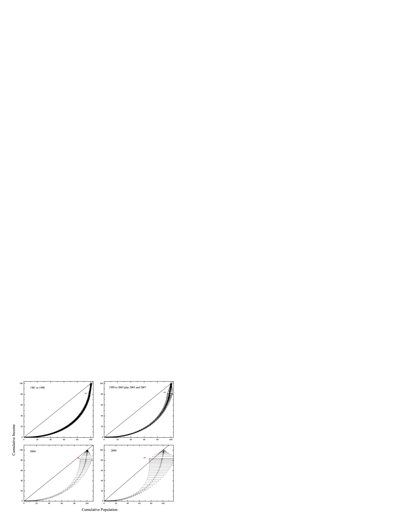
Figure 1: Lorenz curves for Brazil from 1981 to 2007 obtained by using the GPD parameters of Table 1 in equations (25) and (26). The small arrows indicate the approximate point of transition from the Gompertz region to the power-law regime. Vertical and horizontal error bars represent uncertainties calculated by standard error propagation techniques. They are divided in two groups according to how well similar curves collapse to a single curve. The top left graph shows the curves from 1981 to 1998, whereas the top right plot presents the Lorenz curves from 1999 to 2007, except 2004 and 2006 which are both shown separately at the bottom. The plots themselves show clearly that, excluding 2004 and 2006, all other curves fall in two distinct groups, since the collapsed curves become very well defined. The Brazilian Lorenz curves present a remarkable stability in their respective time frames, even considering the hyperinflation period, which is included in the top left plot. The graphs for 2004 and 2006 are shown individually at the bottom because in these volatility is highest. This is a consequence of the fact that the Brazilian agency responsible for collecting income data carried out a much more restricted sampling in those years, resulting in much shorter Pareto tails and, hence, higher fluctuations, as compared to the other years. Since the Gompertz curve is a double exponential, larger fluctuations are greatly amplified at the middle upper range of the Gompertzian section of the distribution.

The results for the Gini coefficient and the percentage share of the Gompertzian part obtained by using the parameters $\alpha$, $x_{t}$ and $B$ of Table 1 in equations (27) and (29) are shown at the last two columns on the right in Table 1. These were calculated by assuming the GPD and are shown as $Gini^{*}$ and $u^{*}$. Uncertainties were also calculated by standard error propagation techniques, but should not be viewed at their face values, but just as general indications of error margins since we are not dealing with experimental errors stemming from experimental devices in carefully controlled environments available in laboratories where measurement limitations can be precisely determined. However, one can see by comparing $Gini$ with $Gini^{*}$ and $u$ with $u^{*}$ that in general the calculations recover both quantities, indicating an overall consistency between the GPD and the individual income data of Brazil from 1981 to 2007.

Figure 2 shows a plot for both original $Gini$ and calculated $Gini^{*}$ coefficients appearing in Table 1. One can verify a general agreement between both results, indicating a good consistency between the GPD and the Brazilian personal income data in the studied time span. A better comparison is shown in Fig. 3 where the curves were zoomed in and error bars removed for better clarity. It is clear from this plot that our calculated $Gini^{*}$ values were systematically overestimated as compared the original $Gini$. However, this difference is small, having a maximum discrepancy of 7%. That might be a result of a possible statistical bias, probably present in the original estimation of the GPD parameters. In any case, one can verify a general agreement in the evolving tendency of the two curves. From 1983 to 1993 there are visible high fluctuations in the original Gini coefficients, a period which is within the high inflationary period Brazil went through by the end of the last century. In fact, the peak of this period is 1989, when Brazil suffered from hyperinflation reaching almost three digits per month. After 1994, the year when inflation came to an abrupt end, the two lines tend to follow each other with a systematic, but stable, difference.

Figure 2: Plots comparing the original Gini coefficients with the calculated ones in Table 1. One can see a general agreement between both sets of points, indicating consistency between the GPD and Brazil’s personal income data in the period analyzed here.

Figure 3: This graph shows the same results of Fig. 2, but zoomed in and without error bars for better clarity. High fluctuations can be seen from 1983 to 1993 in the original $Gini$ values, a period which coincides with very high inflation, peaking with hyperinflation in 1989, the highest peak of the lower curve. The plot also shows a systematic difference between both lines for most of the studied time span, varying mostly from 0.02 to 0.03 and reaching its maximum of 0.041 in 1992 which is within the strong inflationary period Brazil experienced at that time. Despite this systematic difference, which might be a result of some statistical bias present in the original determination of the GPD parameters, one can observe a general consistency between both curves, especially if we bear in mind that this discrepancy does not go higher than a 7%, a value which could possibly be taken as the upper limit of this possible bias.

The results for the percentage share of the Brazilian population whose income is inside the Gompertzian part of the distribution are shown in Fig. 4. There we can see again a general consistency between the original $u$ values with the calculated $u^{*}$ of Table 1. Figure 5 shows the same results, but zoomed in and without error bars. Similarly to the Gini coefficients, one can verify a systematic difference between both lines, but now the calculated values $u^{*}$ are underestimated as compared to the original ones. We can again see high fluctuations in the original values from 1988 to 1994, a period within the high inflationary era in Brazil. The deepest valley occurs in 1989, the year of highest hyperinflation in Brazil. Nevertheless, the two curves tend to evolve in a similar fashion, also featuring an approximately stable discrepancy whose maximum is 6%.

Figure 4: This graph shows the evolution of $u$, the percentage share of the total income of the Gompertzian part of the distribution, originally obtained without assuming the GPD, as compared with the calculated ones listed as $u^{*}$ in Table 1 and obtained using the fitted GPD parameters. Similarly to the case of the Gini coefficients, one can see a general consistency between both results, although a systematic discrepancy is also present (see Fig. 5).

Figure 5: This graph shows the same results of Fig. 4, but zoomed in and with error bars removed for better clarity. We can verify that there is a systematic underestimation of the calculated results for $u^{*}$ as compared to the original ones listed as $u$ in Table 1. This discrepancy has, however, a maximum value of 6%, being, therefore, very close to the one found in the Gini coefficients (see Fig. 3). One can also see high fluctuations in the original results during the inflationary period of Brazil. However, here these fluctuations seem to be restricted to the somewhat shorter period lasting from 1988 to 1994. The deepest valley occurs in 1989, the year when Brazil was hit by hyperinflation. Since this systematic discrepancy is small and mostly stable, the results indicate that overall the GDP provides a good and consistent way of modeling income distribution data.

As final comments, one may ask if a combined two-part function is more appropriate to describe income distribution rather than a single function, no matter how complicated. It was argued in Ref. [28] that from an econophysical viewpoint the paramount objective of an accurate empirical characterization of income distribution is to reveal the underlying dynamics of this system and its governing differential equations. On this point one should mention the model advanced by Scafetta et al. [34] [see also 56, 57] where the distribution of wealth, not income, can be explained by a two-part function, where the low to medium range is fitted to the gamma function and the high wealth is fitted to the Pareto power-law. If the less wealthy has in trade the origin of their resources, with trade being statistically biased in favor of the poor, and the rich obtain their resources from investment, then the model reproduces the stratification of society into a small upper class comprising about 1% of the population and the remaining 99% forming a large middle class together with a poor class. So, two functions mean two different, but inter-related, dynamics: the gamma function would represent returns in trade and the Pareto power-law returns in investment. So, the less wealthy trade with an advantage their only low-return resource, their own labor.

To reach these conclusions, Ref. [34] developed a stochastic model built upon some economic concepts which may provide useful in further studies of the dynamics of income distribution. Thus, wealth should not be confused with income, since, although related, the former comprises all assets and liabilities of a person reported at a certain moment, e.g., at the person’s death, whereas income is the quantity of money, or its equivalent, a person receives in a certain period of time in exchange for sale of goods or property, services, labor or profit from financial investments. So, similarly to [28], it seems reasonable to state that income is a flux of money, or its equivalent, per time unit, whereas wealth could be thought of as income less consumption integrated over a period of time plus a constant representing assets obtained in a previous time period. In addition, Scafetta et al. [34] define investment as “any act that creates or destroys wealth” and trade as “any type of economic transaction.” Accordingly, in a trade transaction the total wealth is conserved and the rich receive their returns from investments as they own the means of large production. They conclude by arguing that this trade bias in favor of the poor is not only possible, but necessary so that society is stabilized in order to avoid the catastrophic situation where the entire wealth of the society becomes concentrated in the hands of very few extremely wealthy people.

Therefore, a two-part function may provide important hints to the underlying dynamics of income distribution, hints on the relationship between the upper and lower sections of the distribution function which would otherwise remain hidden if one were to use a single distribution function. This seems specially true when one considers that society is formed by economically distinct classes that may be better represented by distinct functions, which in turn possess distinct, but inter-related, dynamics.

5 Conclusions

In this paper we have studied the Gompertz-Pareto distribution (GPD), formed by the combination of the Gompertz curve, representing the overwhelming majority of the economically less favorable part of the population of a country, and the Pareto power law, describing its tiny richest part. We discussed how the GPD is fully characterized by only three positive parameters, inasmuch as boundary and continuity conditions limit the parametric freedom of this distribution, and which can be determined by linear data fitting. Equations for the cumulative income distribution, complementary cumulative income distribution, income probability density, Lorenz curve, Gini coefficient and the percentage share of the Gompertzian part were all written in this distribution. We discussed how the GPD allows for an exponential approximation in its middle and upper sections outside the Paretian region.

Application of this income distribution function was made to the Brazilian data from 1981 to 2005, previously published by Moura Jr. and Ribeiro [28], with additional new results for 2006 and 2007. Consistency tests were carried out by comparing the Gini coefficients obtained directly from the original data, without any assumption for the shape and form of the distribution, with results obtained by using the fitted parameters in order to re-obtain those coefficients. Similar tests were made with the values of the percentage share of the Gompertzian part of the distribution. The results indicate a general consistency between the original values of both quantities as compared to the calculated ones using the GPD parameters, although we found a systematic, but mostly stable, discrepancy between these quantities in the range of 6% to 7%. This small discrepancy might be due to some statistical bias possibly present in the original calculation of the GPD parameters of Brazil.

In conclusion, the results presented in this paper suggest that the GPD does provide a coherent and analytically simple representation for income distribution data leading to consistent results, at least as far as data from Brazil is concerned.

We are grateful to 4 referees for their useful comments and suggestions, as well as for pointing out various interesting papers which at the time of writing the first version of this article we were unaware of.

References

- [1] V. Pareto, “Cours d’Économie Politique”, Lausanne, 1897
- [2] N.C. Kakwani, “Income Inequality and Poverty”, Oxford University Press, 1980
- [3] M. Gallegati, S. Keen, T. Lux, P. Ormerod, “Worrying Trends in Econophysics”, Physica A, 370 (2006) 1
- [4] J. Doyne Farmer, M. Shubik, E. Smith, “Is Economics the Next Physical Science?”, Physics Today, September (2005) 37-42, arXiv:physics/0506086v1
- [5] C. Schinckus, “Economic Uncertainty and Econophysics”, Physica A, 388 (2009) 4415-4423
- [6] C. Schinckus, “Econophysics and Economics: Sister Disciplines?”, Am. J. Phys., 78 (2010) 325-327
- [7] C. Schinckus, “Is Econophysics a New Discipline? The Neopositivist Argument”, Physica A, in press (2010), doi:10.1016/j.physa.2010.05.016
- [8] E. Fullbrook, “Introduction: Broadband versus Narrowband Economics”. In “A Guide to What’s Wrong with Economics”, E. Fullbrook (ed.), pp. 1-6, Anthem Press: London, 2004
- [9] P. Söderbaum, “Economics as Ideology and the Need for Pluralism”. In “A Guide to What’s Wrong with Economics”, E. Fullbrook (ed.), pp. 158-168, Anthem Press: London, 2004
- [10] J.-P. Bouchaud, “Economics Needs a Scientific Revolution”, Nature, 455 (2008) 1181; Real-World Economics Review, 48 (2008) 291-292, http://www.paecon.net/PAEReview/issue48/Bouchaud48.pdf, arXiv:0810.5306v1
- [11] S. Keen, “Debunking Economics”, Zed Books: London, 2001
- [12] S. Keen, “Standing on the Toes of Pygmies: Why Econophysics Must Be Careful of the Economic Foundations on Which It Builds”, Physica A, 324 (2003) 108
- [13] S. Keen, “Improbable, Incorrect or Impossible: the Persuasive but Flawed Mathematics of Microeconomics”. In “A Guide to What’s Wrong with Economics”, E. Fullbrook (ed.), pp. 209-222, Anthem Press: London, 2004
- [14] A. Kirman, “Economic Theory and the Crisis”, Real-World Economics Review, 51 (2009) 80-83, http://www.paecon.net/PAEReview/issue51/Kirman51.pdf
- [15] B.B. Mandelbrot, R.L. Hudson, “The (Mis)Behavior of Markets”, Basic Books: New York, 2004
- [16] P. Ormerod, “The Death of Economics”, Wiley: New York, 1997
- [17] P. Ormerod, “The Current Crisis and the Culpability of Macroeconomics”, preprint, (2009), http://www.paulormerod.com/pdf/accsoct09br.pdf
- [18] D. Colander, H. Fölmer, M. Goldberg, A. Haas, K. Juselius, A. Kirman, T. Lux, B. Sloth, “The Financial Crisis and the Systemic Failure of Academic Economics”, Critical Review, 21 (2009) nos. 2-3, http://www.debtdeflation.com/blogs/wp-content/uploads/papers/Dahlem_Report_EconCrisis021809.pdf
- [19] J.-P. Bouchaud, “The (Unfortunate) Complexity of the Economy”, Physics World, April (2009) 28-32, arXiv:0904.0805v1
- [20] A. Drăgulescu, V.M. Yakovenko, “Evidence for the Exponential Distribution of Income in the USA”, Eur. Phys. J. B, 20 (2001) 585, arXiv:cond-mat/0008305v2
- [21] A. Christian Silva, “Applications of Physics to Finance and Economics: Returns, Trading Activity and Income”, PhD thesis, University of Maryland, 2005, arXiv:physics/0507022v1
- [22] V.M. Yakovenko, J.B. Rosser, “Colloquium: Statistical Mechanics of Money, Wealth, and Income”, Rev. Mod. Phys., 81 (2009) 1703-1725, arXiv:0905.1518v2
- [23] A. Chatterjee, B.K. Chakrabarti, S.S. Manna, “Pareto Law in a Kinetic Model of Market with Random Saving Propensity”, Physica A, 335 (2004) 155
- [24] F. Clementi, M. Gallegati, G. Kaniadakis, “k-Generalised Statistics in Personal Income Distribution” Eur. Phys. J. B, 57 (2007) 187-193, arXiv:physics/0607293v2
- [25] F. Clementi, T. Di Matteo, M. Gallegati, G. Kaniadakis, “The k-Generalised Distribution: a New Descriptive Model for the Size Distribution of Incomes”, Physica A, 387 (2008) 3201-3208, arXiv:0710.3645v4
- [26] F. Clementi, M. Gallegati, G. Kaniadakis, “A k-Generalized Statistical Mechanics Approach to Income Analysis”, J. Stat. Mech., February (2009) P02037, arXiv:0902.0075v2
- [27] G. Willis, J. Mimkes, “Evidence for the Independence of Waged and Unwaged Income, Evidence for Boltzmann Distributions in Waged Income, and the Outlines of a Coherent Theory of Income Distribution”, e-print (2004), arXiv:cond-mat/0406694v1
- Moura Jr. and Ribeiro [2009] N.J. Moura Jr., M.B. Ribeiro, “Evidence for the Gompertz Curve in the Income Distribution of Brazil 1978-2005”, Eur. Phys. J. B, 67 (2009) 101-120, arXiv:0812.2664v1
- [29] S. Solomon, “Stochastic Lotka-Volterra Systems of Competing Auto-Catalytic Agents Lead Generically to Truncated Pareto Power Wealth Distribution, Truncated Levy Distribution of Market Returns, Clustered Volatility, Booms and Crashes”. In “Computational Finance 97”, A-P.N. Refenes, A.N. Burgess, J.E. Moody (eds), Kluwer Academic Publishers, 1998, arXiv:cond-mat/9803367v1
- [30] J.-P. Bouchaud, M. Mézard, “Wealth Condensation in a Simple Model of Economy”, Physica A, 282 (2000) 536-545, arXiv:cond-mat/0002374v1
- [31] S. Solomon, P. Richmond, “Power Laws of Wealth, Market Order Volumes and Market Returns”, Physica A, 299 (2001) 188-197, arXiv:cond-mat/0102423v2
- [32] P. Repetowicz, S. Hutzler, P. Richmond, “Dynamics of Money and Income Distributions”, Physica A, 356 (2005) 641-654, arXiv:cond-mat/0407770v1
- [33] R. Coelho, P. Richmond, J. Barry, S. Hutzler, “Double Power Laws in Income and Wealth Distributions”, Physica A, 387 (2008) 3847-3851, arXiv:0710.0917v1
- [34] N. Scafetta, S. Picozzi, B.J. West, “An Out-of-Equilibrium Model of the Distribution of Wealth”, Quantitative Finance, 4 (2004) 353-364, arXiv:cond-mat/0403045v1
- [35] A. Banerjee, V.M. Yakovenko, “Universal Patterns of Inequality”, New J. Phys., in press (2010), arXiv:0912.4898v4
- [36] M.B. Ribeiro, A.Y. Miguelote, “Fractals and the Distribution of Galaxies”, Brazilian J. Phys., 28 (1998) 132-160, arXiv:astro-ph/9803218v1
- [37] A. Gabrielli, F. Sylos Labini, M. Joyce, L. Pietronero, “Statistical Physics for Cosmic Structures”, Springer: Berlin, 2005
- [38] M.B. Ribeiro, “On Modeling a Relativistic Hierarchical (Fractal) Cosmology by Tolman’s Spacetime. I. Theory”, Astrophys. J., 388 (1992) 1-8, arXiv:0807.0866v1
- [39] M.B. Ribeiro, “On Modeling a Relativistic Hierarchical (Fractal) Cosmology by Tolman’s Spacetime. III. Numerical Results”, Astrophys. J., 415 (1993) 469-485, arXiv:0807.1021v1
- [40] M.B. Ribeiro, “Relativistic Fractal Cosmologies”. In “Deterministic Chaos in General Relativity”, D.W. Hobill, A. Burd, A. Coley (eds.), pp. 269-296, Plenum Press: New York, 1994, arXiv:0910.4877v1
- [41] E. Abdalla, R. Mohayaee, M.B. Ribeiro, “Scale Invariance in a Perturbed Einstein-de Sitter Cosmology”, Fractals, 9 (2001) 451-462, arXiv:astro-ph/9910003v4
- [42] M.B. Ribeiro, “Cosmological Distances and Fractal Statistics of Galaxy Distribution”, Astron. Astrophys., 429 (2005) 65-74, arXiv:astro-ph/0408316v2
- [43] V.V.L. Albani, A.S. Iribarrem, M.B. Ribeiro, W.R. Stoeger, “Differential Density Statistics of the Galaxy Distribution and the Luminosity Function”, Astrophys. J., 657 (2007) 760-772, arXiv:astro-ph/0611032v1
- [44] B.M. Boghosian, “Thermodynamic Description of the Relaxation of Two-Dimensional Turbulence Using Tsallis Statistics”, Phys. Rev. E, 53 (1996) 4754
- [45] S. Redner, “How Popular is your Paper? An Empirical Study of the Citation Distribution”, Eur. Phys. J. B, 4 (1998) 131
- [46] D.C. Roberts, D.L. Turcotte, “Fractality and Self-Organized Criticality of Wars”, Fractals, 6 (1998) 351-357
- [47] J. Alvarez-Ramirez, C. Ibarra-Valdeza, E. Rodriguez, R. Urrea, “Fractality and Time Correlation in Contemporary War”, Chaos, Solitons & Fractals, 34 (2007) 1039-1049
- [48] J. Alvarez-Ramirez, E. Rodriguez, R. Urrea, “Scale Invariance in the 2003-2005 Iraq Conflict”, Physica A, 377 (2007) 291-301
- [49] N.J. Moura Jr., M.B. Ribeiro, “Zipf Law for Brazilian Cities”, Physica A, 367 (2006) 441-448, arXiv:physics/0511216v2
- [50] X. Gabaix, P. Gopikrishnan, V. Plerou, H. Eugene Stanley, “A Theory of Power-Law Distributions in Financial Market Fluctuations”, Nature, 423 (2003) 267
- [51] K.J. Niklas, “Size-Dependent Variations in Plant-Growth Rates and 3/4-Power Rules”, Amer. J. Botany, 81 (1994) 134
- [52] J.C. Nacher, T. Ochial, “Power-Law Distribution of Gene Expressions Fluctuations”, Phys. Lett. A, 272 (2008) 6202
- [53] G.B. West, J.H. Brown, “Life’s Universal Scaling Laws”, Physics Today, September (2004) 36-42
- [54] M.E.J. Newman, “Power Laws, Pareto Distributions and Zipf’s Law”, Contemporary Phys., 46 (2005) 323-351, arXiv:cond-mat/0412004v3
- [55] G. Kaniadakis, “Maximum Entropy Principle and Power-Law Tailed Distributions”, Eur. Phys. J. B, 70 (2009) 3-13, arXiv:0904.4180v2
- [56] N. Scafetta, S. Picozzi, B.J. West, “Pareto’s Law: a Model of Human Sharing and Creativity”, e-print, (2002), arXiv:cond-mat/0209373v1
- [57] N. Scafetta, S. Picozzi, B.J. West, “A Trade-Investment Model for Distribution of Wealth”, Physica D, 193 (2004) 338-352, arXiv:cond-mat/0306579v2