Laboratoire de Physique Théorique de l’École Normale Supérieure École Doctorale de Physique la Région Parisienne — ED 107 Physique l’Université Pierre et Marie CURIEUNIVERSITE PIERRE ET MARIE CURIE [M]Rémi Monasson et Nicolas Sourlas [M] [Mme]Leticia CugliandoloPrésident du jury
[M]John HertzRapporteur
[M]Silvio FranzRapporteur
[M]Florent KrzakalaExaminateur
[M]Rémi MonassonDirecteur de Thèse
[M]Nicolas SourlasInvité

Problèmes inverses dans les modèles de spin

Un bon nombre d’exp riences r centes en biologie mesurent des syst mes compos s de plusieurs composants en interactions, comme par exemple les r seaux de neurones. Normalement, on a exp rimentalement acc s qu’au comportement collectif du syst me, m me si on s’int resse souvent la caract risation des interactions entre ses diff rentes composants. Cette th se a pour but d’extraire des informations sur les interactions microscopiques du syst me partir de son comportement collectif dans deux cas distincts. Premi rement, on tudie un syst me d crit par un mod le d’Ising plus g n ral. On trouve des formules explicites pour les couplages en fonction des corr lations et magn tisations. Ensuite, on s’int resse un syst me d crit par un mod le de Hopfield. Dans ce cas, on obtient non seulement une formule explicite pour inf rer les patterns, mais aussi un r sultat qui permet d’estimer le nombre de mesures n cessaires pour avoir une inf rence pr cise. Several recent experiments in biology study systems composed of several interacting elements, for example neuron networks. Normally, measurements describe only the collective behavior of the system, even if in most cases we would like to characterize how its different parts interact. The goal of this thesis is to extract information about the microscopic interactions as a function of their collective behavior for two different cases. First, we will study a system described by a generalized Ising model. We find explicit formulas for the couplings as a function of the correlations and magnetizations. In the following, we will study a system described by a Hopfield model. In this case, we find not only explicit formula for inferring the patterns, but also an analytical result that allows one to estimate how much data is necessary for a good inference.

Remerciements

Si je devais remercier tous ceux dont j’ai envie, cette liste serait beaucoup trop longue. Je fais alors le compromis de me restreindre ceux que j’ai crois quotidiennement pendant ma th se (ou pendant une p riode).

Tout d’abord, je voudrais remercier R mi Monasson de m’avoir fait d couvrir tous les domaines forts int ressants dans lesquels j’ai travaill pendant ma th se. Merci galement d’avoir t aussi efficace afin de me d bloquer quand je n’arrivais pas au bout d’un calcul. Finalement, je lui suis tr s reconnaissant de m’avoir donn l’occasion de travailler dans le cadre tr s exceptionnel de l’IAS et pour toutes les d marches faites pour faciliter mon installation aux USA.

J’aimerais aussi remercier Simona Cocco pour toutes les discussions tr s fructueuses et de m’avoir aider sur ma th se plusieurs reprises.

Une autre personne que je ne peux pas oublier est Stan Leibler. Merci de m’avoir si bien accueilli l’IAS et de m’avoir donner l’occasion d’exposer mon travail son groupe.

Un merci galement tr s particulier Carlo pour toute son aide et sa patience pendant notre collocation Princeton et d’avoir t un ami de toute heure aussi bien Paris qu’ Princeton. Merci aussi Laeticia pour sa compagnie.

J’en profite pour remercier Stan, R mi, Simona, Carlo, Laetitia et Arvind pour tous les d jeuners relaxants Princeton.

Un merci particulier galement John Hertz, de m’avoir invit pour faire un s minaire et de son accueil chaleureux Stockholm.

Je n’oublie pas mes coll gues de bureau et d’ tage : merci Florent d’ tre toujours de bonne humeur et d’avoir toujours des choses int ressantes dire; merci tous les th sards de la g ophysique, pour les d jeuners dans une tr s bonne ambiance; et merci Sebastien d’ tre un coll gue de bureau tr s sympathique.

Je voudrais aussi remercier ma famille d’avoir t si patiente pendant toutes ces longues ann es d’absence et de m’avoir toujours encourag . Finalement, je veux remercier de tout mon cœur Camilla, d’avoir toujours t de mon c t pendant toutes ces ann es ensemble, d’avoir toujours t si patiente dans mes moments de mauvaise humeur et d’avoir accept si patiemment mes longues absences l’ tranger.

Contents

1. I Introduction
   1. 1 Biological motivation and related models
      1. 1.1 Neuron networks
         1. 1.1.1 Multi-neuron recording experiments
         2. 1.1.2 Models for neuron networks
      2. 1.2 Homologous proteins
   2. 2 Some classical results on Ising-like models
      1. 2.1 The Ising model
      2. 2.2 Sherrington-Kirkpatrick model
         1. 2.2.1 Replica solution of the SK model
      3. 2.3 TAP Equations
      4. 2.4 Hopfield model
      5. 2.5 Graphical models
         1. 2.5.1 Message-passing algorithms
   3. 3 Inverse Problems
      1. 3.1 Maximal entropy distribution
      2. 3.2 Bayesian inference
         1. 3.2.1 Relationship with entropy maximization
      3. 3.3 The I.I.P.: some results from the literature
         1. 3.3.1 Monte Carlo optimization
         2. 3.3.2 Susceptibility propagation
         3. 3.3.3 Inversion of TAP equations
         4. 3.3.4 Auto-consistent equations
2. II Some results on the inverse Ising problem
   1. 4 The inverse Ising problem in the small-correlation limit
      1. 4.1 Evaluation of S¹ and S²
      2. 4.2 Evaluation of S³
      3. 4.3 Higher orders
      4. 4.4 Checking the correctness of the expansion
         1. 4.4.1 Comparing the values of the external field with TAP equations
         2. 4.4.2 Numerical minimum-squares fit
   2. 5 Further results based on our expansion for the inverse Ising model
      1. 5.1 Loop summation
      2. 5.2 Combining the two-spin expansion and the loop diagrams
         1. 5.2.1 Three spin diagrams
      3. 5.3 Quality of the inference after summing the loops and 2-3 spin diagrams
         1. 5.3.1 One-dimensional Ising
         2. 5.3.2 Sherrington-Kirkpatrick model
      4. 5.4 Numerical evaluation of high-order diagrams
      5. 5.5 Expansion in n-spin diagrams
3. III Inference of Hopfield patterns
   1. 6 Pattern inference for the Hopfield model
      1. 6.1 A simpler case: inference of a single pattern
         1. 6.1.1 Ferromagnetic case
         2. 6.1.2 Paramagnetic case
      2. 6.2 Inference of continuous patterns for p ¿ 1
         1. 6.2.1 Discussion on the gauge
         2. 6.2.2 Ferromagnetic phase
         3. 6.2.3 High external field case
         4. 6.2.4 Numerical verification
   2. 7 Evaluation of the inference entropy for the Hopfield model
      1. 7.1 Case of a single binary pattern
         1. 7.1.1 Ferromagnetic case
         2. 7.1.2 Paramagnetic case
      2. 7.2 Case of a single pattern $\xi_{i}\in\mathbb{R}$
      3. 7.3 Case of a system with p patterns, magnetized following a strong external field
      4. 7.4 Two patterns, magnetized according to the first
         1. 7.4.1 Evaluation of $\bm{\langle}$log Ñ$\bm{\rangle}$
   3. 8 Conclusion
   4. A Details of the small-$\bm{\beta}$ expansion
      1. A.1 Second order expansion
      2. A.2 Third order expansion
   5. B Large magnetization expansion
   6. C Verification of h_i({c},{m})
      1. C.1 Evaluation of h_i⁽³⁾({J})
      2. C.2 Evaluation of h_i⁽³⁾({c})
      3. C.3 Evaluation of h_i⁽⁴⁾({J})
      4. C.4 Evaluation of h_i⁽⁴⁾({c})
   7. D Evaluation of $\log Z$
   8. E Evaluation of m for the entropy of the Ising model
   9. F Evaluation of Ñ in the paramagnetic phase
   10. G Entropy calculations details for continuous patterns
   11. H Details of the evaluation of the entropy for the Hopfield model
   12. I Details of the evaluation of $\bm{\langle}$Ñ$\bm{\rangle}$ for the Hopfield model with large h
       1. I.1 Determination of log Z${}_{\text{Hop}}$
       2. I.2 Determination of $\left\langle\log\tilde{N}\right\rangle$

Part I Introduction

Chapter 1 Biological motivation and related models

In the last years, we have seen a remarkable growth in the number of experiments in biology that generate an overwhelming quantity of data. In several cases, like in neuron assemblies, proteins and gene networks, most of the data analysis focuses on identifying correlations between different parts of the system. Unfortunately, identifying the correlations on their own is only of limited scientific value: most of the underlying properties of the system can only be understood by describing the interaction between their different parts. This work finds its place in developing statistical mechanics tools to derive these interactions from measured correlations.

In this introductory chapter, we present two biological problems that inspired this thesis. First, in section 1.1 we give a brief introduction to neurons and how they exchange information in a network. We discuss some experiments where the individual activity of up to a hundred interacting neurons is measured. For this example, the neurons are the interacting parts and they interact via synapses, whose details are very hard to extract experimentally.

In a second part, we discuss some recent works on the analysis of families of homologous proteins, i. e., proteins that share an evolutionary ancestry and function. The variation of the amino acids inside these families are highly correlated which is deeply related to the biological function of the proteins. In general terms, we can say thus that individual amino acid variations play the role of interacting parts with very complicated interactions, as we will see in section 1.2.

1.1 Neuron networks

One of the most important scientific questions of the 21st century is the understanding of the brain. It is widely accepted that its complexity is due to the organization of neurons in complex networks. If we consider, for example, the human brain, we can count about $10^{11}$ neurons connected by about $10^{14}$ connections. Even much simpler organisms like the Drosophila melanogaster fruit fly counts about 100,000 neurons.

A typical neuron can be schematized as a cell composed of three parts: the cell body, dendrites and one axon (see Fig. 1.1). A dendrite is composed of several branches in a tree-like structure and is responsible for receiving electric signals from other neurons. The axon is a longer, ramified single filament, responsible for sending electrical signals to other neurons. A connexion between two neurons in most cases happens between an axon and a dendrite. We call such connections synapses.

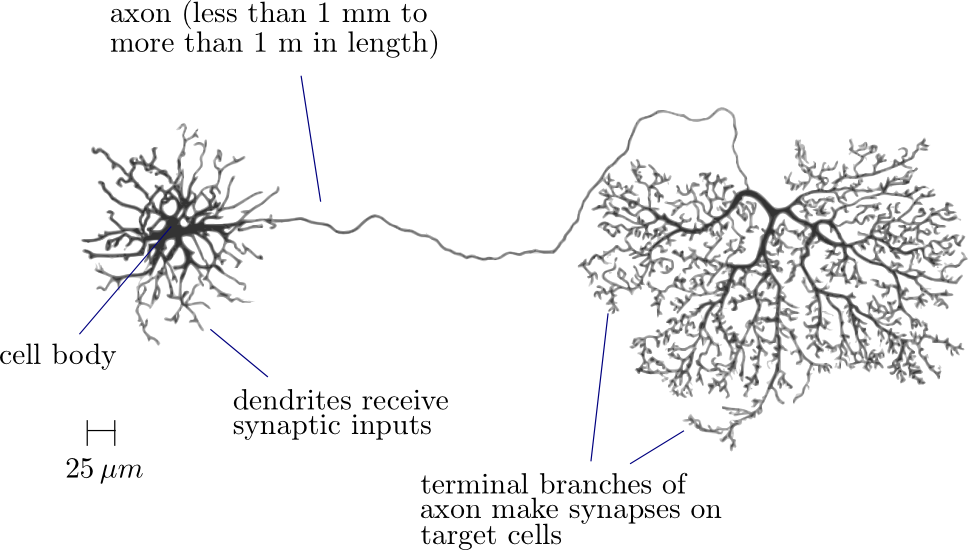
Figure 1.1: Schema of a neuron [Alberts 02]. The diameter of the cell body is typically of the order of $10\,\mu m$, while the length of dendrites and axons varies considerably with the neuron’s function.

Like most cells, neurons have an electrical potential difference between their cytoplasm and the extracellular medium. This potential difference is regulated by the exchange of ions (such as $\text{Na}^{+}$ and $\text{K}^{+}$) through the cell membrane, which can be done in two ways: passively, by proteins called ion channels that selectively allow the passage of a certain ion from the most concentrated medium to the least and, conversely, actively by proteins called ion pumps that consume energy to increase the ion concentration difference.

A typical neuron has a voltage difference of about $-70\,mV$ when it is not receiving any signal from other neurons. We call this voltage the resting potential of the neuron. If the voltage of a neuron reaches a threshold (typically about $-50\,mV$), a feedback mechanism makes ion channels of the membrane to open, making the voltage increase rapidly up to $100\,mV$ (depending on the neuron type), after which it reaches saturation and decreases quickly, recovering the resting potential after a few $ms$ (see Fig. 1.2). We call this process firing or spiking. One important characteristic of the spikes is that once the voltage reaches the threshold, its shape and its intensity do not depend on the details of how the threshold was attained.

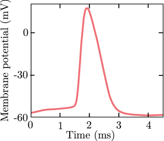
Figure 1.2: Typical voltage as a function of time graph for a firing neuron [Naundorf 06].

When a neuron fires, its axon releases neurotransmitters at every synapse. Those neurotransmitters make ions channels in the dendrites open, changing the membrane potential of the neighboring neurons. Different neurotransmitters cause the opening of different ion channels, allowing for both excitatory synapses, which increase the neuron potential, and inhibitory synapses which decrease it. Since synapses can be excitatory or inhibitory to different degrees, most models define a synaptic weight with the convention that excitatory synapses have a positive synaptic weight and inhibitory synapses have a negative one, as we will see in section 1.1.2. Another important feature of synapses is that they are directional: if a neuron $A$ can excite a neuron $B$, the converse is not necessarily true: neuron $B$ might inhibit neuron $A$, or simply not be connected to it at all.

1.1.1 Multi-neuron recording experiments

While much progress has been done in describing individual neurons, understanding their complex interaction in a network is still an unsolved problem. One of the most promising advances in this area was the development of techniques for recording simultaneously the electrical activity of several cells individually [Meister 94].

In these experiments, a microarray counting as many as 250 electrodes is placed in contact with the brain tissue. The potential of each electrode is recorded for up to a few hours. Each one of the electrodes might be affected by the activity of more than one neuron and, conversely, a single neuron might affect more than one electrode. Thus, a computational-intensive calculation is needed to factorize the signal as the sum of the influence of several different neurons. This procedure is known as Spike Sorting [Peyrache 09] and its results are spike trains, i.e., time sequences of the state of each cell: firing or at rest. An example of a set of spike trains can be seen in Fig. 1.3.

Figure 1.3: Typical measurement of spike trains[Peyrache 09]. Each line corresponds to a single neuron. Black vertical bars correspond to spikes.

In principle, one should be able to pinpoint the synapses and the synaptic weights from the spike trains. However, extracting this information is a considerable challenge. First of all, it is not possible with current technology to measure every neuron of a network. Thus, experiments measure just a small fraction of the system even if the network is small. That means that all that we can expect to find are effective interactions that depend on all links between the cells that are not measured. Secondly, one can not naively state that if the activity of two neurons is correlated then they are connected by a synapse. Consider, for example, neurons 7, 22 and 27 of Fig. 1.3, indicated by the red arrows. We can clearly see that there is a tendency for all three of firing at the same time, but distinguishing between the two possible connections shown in Fig. 1.4 is not trivial.

Figure 1.4: Two different possible configurations for three positively correlated neurons.

1.1.2 Models for neuron networks

Before talking about what have already been done to solve this problem and our contribution to it, we present some models for neural networks. We will proceed by first introducing a model that describes rather faithfully real biological networks, the leaky Integrate-and-Fire model. Afterwards, we introduce the Ising model, which is much more tractable analytically. Finally, we will look at the Ising model from a different point of view by studying one particular case of it: the Hopfield model.

Leaky integrate-and-fire model

The leaky integrate-and-fire model, first proposed by Lapicque in 1907 [Lapicque 07, Abbott 99, Gerstner 02, Burkitt 06], is a straightforward modelization of the firing process presented in section 1.1. It supposes that neurons behave like capacitors with a small leakage term to account for the fact that the membrane is not a perfect insulator. Posing $V(t)$ as the function representing the difference of potential between the inside and the outside of the membrane:

$$C\frac{\mathrm{\;d}V}{\mathrm{\;d}t}=-\frac{V(t)}{R}+I(t)\,,$$ (1.1)

where $C$ is the capacitance of the neuron, $R$ is the resistance of the cell membrane and $I(t)$ is the total current due to the synapses of neighboring neurons. If we introduce the characteristic time of leakage $\tau=RC$, we can rewrite this equation as

$$\tau\frac{\mathrm{\;d}V}{\mathrm{\;d}t}=-V(t)+RI(t)\,.$$ (1.2)

Spikes are modelized solely by their “firing time” $t_{f}$. This firing time is defined as the moment where the neuron’s potential reaches a firing threshold value $V_{tr}$. Implicitly, it is given by the equation

$$V(t_{f})=V_{tr}\,.$$ (1.3)

Every time a neuron spikes, its potential is reset to zero and its synapses produce a signal in the form of some function $f(t)$. We can thus describe the signal $S(t)$ that this neuron send to its neighbors as a function only of the set of firing times $\{t_{f}^{r}\}_{r=1,\ldots,N_{\text{spikes}}}$

$$S(t)=\sum_{r=1}^{N_{\text{spikes}}}f(t-t_{f}^{r})\,.$$ (1.4)

The choice of the function $f(t)$ can be based on biological measures, mimicking the behavior shown in Fig. 1.2 or can be a simple Dirac-delta function to make calculations easier.

Finally, we can introduce the synaptic weights to model a neuron network with the following equations:

$$\tau_{i}\frac{\mathrm{\;d}V_{i}}{\mathrm{\;d}t} = -V_{i}(t)+\sum_{j}J_{ij}S_{j}(t)\,,$$ (1.5)

$$V_{i}(t_{f}^{i,r}) = 1\,,$$ (1.6)

$$S_{i}(t) = \sum_{r=1}^{N_{\text{spikes}}^{i}}f(t-t_{f}^{i,r})\,,$$ (1.7)

where $V_{i}$ is the potential of the neuron $i$ rescaled so that $V_{tr}=1$, $t_{f}^{i,r}$ is the time of the $r$-th spike of the neuron $i$ and $J_{ij}$ is the matrix of the synaptic weights. Note that it is usually assumed as an approximation that the function $f(t)$ is identical for all neurons.

This model is very popular due to its balance between biological accuracy and relative simplicity. It is also very well-suited for computer simulations by the direct integration of its differential equations. On the other hand, while some numerical work has been done on the inference of synaptic weights from spike trains using this model [Cocco 09], it is not very practical for analytical results.

Generalized Ising model / Boltzmann Machine

The Boltzmann Machine [McCulloch 43] is a model of neuron networks that mimics less well real biological systems than the leaky Integrate-and-Fire model. It is however considerably simpler, being even exactly solvable for some special networks. In this model, the state of a neuron is fully described by a spin variable $\sigma=\pm 1$ with the convention of $\sigma=+1$ if the neuron is firing and $\sigma=-1$ if it is not. The dynamics of the system is ignored and we describe only the probability $P(\{\sigma_{1},\ldots,\sigma_{N}\})$ of finding the network of $N$ neurons in a state $\{\sigma_{1},...,\sigma_{N}\}$, which is given by the Boltzmann weight of a generalized Ising model

$$P(\{\sigma_{1},...,\sigma_{N}\}) = \frac{1}{Z}e^{-\beta H(\{\sigma_{1},...,\sigma_{N}\})}\,,$$ (1.8)

with

$$Z = \sum_{\{\sigma\}}e^{-\beta H(\{\sigma_{1},...,\sigma_{N}\})}\,,$$ (1.9)

where $Z$ is the partition function of the model, $\beta$ is a parameter of the model, that in the context of spins represents the inverse temperature and we introduced the notation

$$\sum_{\{\sigma\}}\equiv\sum_{\sigma_{1}=\pm 1}\,\sum_{\sigma_{2}=\pm 1}\,\,\cdots\,\,\sum_{\sigma_{N}=\pm 1}\,.$$ (1.10)

The Hamiltonian should take into account the connection between neurons and the fact that some minimum input is needed for the neuron to reach the threshold and fire. The widely used expression is

$$H(\{\sigma_{1},...,\sigma_{N}\}) = -\frac{1}{2N}\sum_{i,j}J_{ij}\sigma_{i}\sigma_{j}-\sum_{i}h_{i}\sigma_{i}\,,$$ (1.11)

where $J_{ij}$ corresponds to the synaptic weight and $h_{i}$ is a term that models the threshold as a “field” favoring the neuron to be in the rest position.

Two features of this model are particularly pertinent for what follows. First, it is directly defined in the language of statistical physics and allows the use of its framework with no additional complications. Secondly, if one measures the averages $\langle\sigma_{i}\rangle$ and the correlations $\langle\sigma_{i}\sigma_{j}\rangle$ of a spike train, the Boltzmann machine arises naturally as a model consistent with these measurements, as we will discuss in more detail in section 3.1. On the other hand, a significant shortcoming of this model is that synapses are symmetric, i. e., $J_{ij}=J_{ji}$, which is not necessarily true in biological systems.

It is important to note that the Hamiltonian shown in Eq. (1.11) can give rise to a rich diversity of behaviors depending on the choice of $J_{ij}$: ferromagnetism, frustration, glassy systems, etc, as we will see in chapter 2.

Particular case: Hopfield model

Until now, we have presented models for neurons in completely arbitrary neuron networks. In this section we will describe a model that uses the same modelization for neurons we presented in the last section but restricts the synaptic weights $J_{ij}$ to a particular form:

$$J_{ij}=\sum_{\mu=1}^{p}\xi_{i}^{\mu}\xi_{j}^{\mu}\,,$$ (1.12)

where $\xi_{i}^{\mu}$ are real values that we will discuss in the following. This particular case of the generalized Ising model is called the Hopfield model and was proposed to describe a system that stores a given number $p$ of memories and is capable to retrieve them when given a suitable input. The form shown in Eq. (1.12) was chosen so that the Hamiltonian we saw in Eq. (1.11) can be rewritten as

$$H=-\frac{1}{2N}\sum_{\alpha=1}^{p}\left(\sum_{i}\xi_{i}^{\alpha}\sigma_{i}\right)^{2}$$ (1.13)

which has the property that $\sigma_{i}=\mathrm{sign}(\xi_{i}^{\alpha})$ is a local energy minimum for every $\alpha$ if $p\ll N$ and the patterns are more or less orthogonal.

The interpretation of this model as a model for associative memory comes from the fact that, under certain conditions, if our system has an initial configuration similar to one of the vectors $\xi^{\mu}$ it will evolve to the configuration $\sigma_{i}=\mathrm{sign}(\xi_{i}^{\mu})$. In this context, we normally call the $p$ vectors $\{\xi^{1},...,\xi^{p}\}$ memories (or patterns). More rigorously, we will see in section 2.4 that in the limit $N\gg 1$, the system can retrieve up to $\alpha_{c}N$ stored binary patterns with $\alpha_{c}\simeq 0.138$.

The Hopfield model can also be seen as an approximation of the general Boltzmann Machine for a finite-rank $J$ matrix. Indeed, let’s write the eigenvector decomposition of the matrix $J$,

$$J_{ij}=\sum_{\alpha=1}^{N}\lambda_{\alpha}v_{\alpha,i}v_{\alpha,j}\,,$$ (1.14)

with $\{\lambda_{\alpha}\}$ and $\{v_{\alpha,i}\}$ being respectively the eigenvalues and eigenvectors of the matrix $J$. If we truncate this summation up to the first $p$ highest eigenvalues and pose $\xi_{i}^{\alpha}=\sqrt{\lambda_{\alpha}}v_{\alpha,i}$, we find exactly the same equation as Eq. (1.13). On the other hand, the limit of $p=N$ does not make this approximation exact, since Eq. (1.13) cannot account for negative eigenvalues of the matrix $J_{ij}$.

This model got a renewed interest when experimentalists started looking for patterns in spike train recording data. A recent experiment with rats made by Peyrache et al. [Peyrache 09] compared the spike activity of neurons in two different moments: when the rat was looking for food in a maze and when it was sleeping. The main statistical tool used by the authors was the Principal Component Analysis (PCA), i.e., finding the eigenvalues and eigenvectors of the correlation matrix of the measured neuron activity. They showed that the eigenvectors that were the most strongly correlated with neuron activity when the rat was choosing a direction in the maze were revisited during his next sleep. The authors interpreted this finding as the well-known process of memory consolidation during sleep. In part III, we will show that the author’s proceeding of extracting patterns from neural data using the PCA is closely related to fitting spike trains with a Hopfield model.

1.2 Homologous proteins

We say that two different proteins are homologous if they have both a common evolutionary origin[Reeck 87] and a similar sequence, which normally also imply a similar function. The comparison of the proteins of a homologous group gives some valuable insight of which features are really essential for their biological function.

Figure 1.5: A set of 41 sequences containing SH2 domain. Each line correspond to a different protein and each letter correspond to an amino acid, with conserved ones in bold. These sequences were matched using a multiple sequence alignment software[Edgar 04].

The first step while comparing two or more homologous proteins is to align their sequences in a way that maximizes the number of identical basis (see Fig. 1.5). This procedure is known as Multiple Sequence Alignment (MSA) [Lockless 99]. Since during evolution there could have been insertion or deletion of basis, the optimal alignment will involve adding empty spaces to the alignment in an optimal way, what makes the MSA problem NP-complete, i.e., solving it needs a number of operations that grows exponentially with the number of sequences.

It is natural to suppose that the most important parts of a protein should vary significantly less than the least important ones, since most mutations in important parts yield non-functional proteins. Consequently, the most straightforward analysis one can do with aligned sequences is to evaluate how the distribution of amino acids in a given position deviates from a random uniform distribution[Capra 07].

While considering each position separately was proved to be useful for identifying functional groups, a much richer behavior was found by considering pairwise correlation between sites. First of all it has been shown that by taking into account both conservation and correlation one can describe more accurately which sites of proteins are essential for its function than by just considering conservation alone[Lichtarge 96].

Secondly, a remarkable experiment by Russ et al. [Russ 05] created artificial proteins by randomly picking amino acids with a probability distribution that reproduced the averages and the pairwise correlations of a group of homologous natural proteins. He showed that these new proteins fold to a native tertiary structure similar to that of the natural proteins of the group. Conversely, he showed that random proteins that were generated without taking into account correlations do not fold into a well-defined three-dimensional structure, an essential step for a protein to be functional.

Moreover, an interesting paper by Halabi et al. [Halabi 09] showed that the correlation matrix has a particular structure: the amino acids can be separated in disjoint groups (or sectors) that are only correlated to other amino acids inside the same sector. Each sector has a distinct functional role and has evolved practically independently from the others.

Finally, studying the two-basis correlations was shown to be a very good way to infer which pairs of amino acids are spatially close in the three-dimensional structure of the protein [Burger 10]. Yet, some non-trivial work is needed to know if two basis are correlated because they are spatially close one to another or because they are spatially close to a third base, a problem very similar to the one presented in section 1.1.1 for neurons. To solve such a problem, a paper published in 2009 [Weigt 09] proposed a very simplified model to describe a family of proteins composed by $N$ amino acids: it supposes that the proteins that constitute the family are randomly chosen among all possible proteins with length $N$ and that the probability of a given protein is given by:

$$P(A_{1},\ldots,A_{N})=\frac{1}{Z}\exp\left[\sum_{i<j}J_{ij}(A_{i},A_{j})+\sum_{i}h_{i}(A_{i})\right]\,,$$ (1.15)

where $A_{i}\in\{1,\ldots,22\}$ describe the $i$-th amino acid of the protein and $J_{ij}(A_{i},A_{j})$ and $h_{i}(A_{i})$ are real-valued functions. This modelization is very similar to the Ising model we saw above and reduces the problem of finding which basis are actually close in the three-dimensional structure of the protein to the problem of finding which functions $J_{ij}$ and $h_{i}$ of the Hamiltonian best describe a set of measured two-site correlations.

To sum up, in the same way we saw in section 1.1 for neurons, we are dealing with a large number of correlated data where the pairwise correlation plays a special role. While for neurons we wanted to infer a synaptic network, in this case we would be interested in extracting an expression for the effective fitness of the proteins of the group, i.e., a quantity that would say how well a protein performs its biological role as a function of its amino acids sequence.

Chapter 2 Some classical results on Ising-like models

As we have seen in chapter 1, Ising-like models are modelizations of neural networks which are particularly suitable for analytical calculations. In this chapter, we present some classical results for some of these models, such as the Sherrington-Kirkpatrick and the Hopfield model. Since normally most of the behavior of the system can be deduced from the partition function $Z$, it is normally said that a model is “solved” when one evaluates this quantity explicitly. We start by reminding some results for the Ising model as it was originally defined. In the sequence, we will present for both the Hopfield and the Sherrington-Kirkpatrick models the procedure for evaluating $Z$ in general lines, since it will be useful later in chapter 6. Indeed, as we will do similar calculations, the comparison with these classical results will be enlightening.

2.1 The Ising model

The original Ising Model was proposed by Wilhelm Lenz and first studied by Lenz’s PhD student Ernst Ising as a simple model for ferromagnetism and phase transitions. This model supposes that the atoms of a magnet are arranged in a lattice and the spin of each atom $i$ is described by a binary variable $\sigma_{i}=\pm 1$. In addition, it assume that each atom interacts only with its closest neighbors, so we can write the energy of the system as

$$H=-J\sum_{<i,j>}\sigma_{i}\sigma_{j}+h\sum_{i}\sigma_{i}\,,$$ (2.1)

where $J$ is the energy of the interaction between neighbors, favoring spins to be aligned and $h$ corresponds to an external magnetic field. The notation $\sum_{<i,j>}$ means summing over all the pairs $i,j$ where $i$ and $j$ are closest neighbors.

We suppose that the probability of the different states of the system is given by the Boltzmann distribution

$$P(\{\sigma_{1},...,\sigma_{N}\}) = \frac{1}{Z}e^{-\beta H(\{\sigma_{1},...,\sigma_{N}\})}\,,$$ (2.2)

with

$$Z = \sum_{\{\sigma\}}e^{-\beta H(\{\sigma_{1},...,\sigma_{N}\})}\,,$$ (2.3)

where $\beta=\frac{1}{k_{\mathrm{B}}T}$, $k_{\mathrm{B}}$ is the Boltzmann constant and $T$ is the temperature. In the following, unless explicitly stated, we will absorb the constant $\beta$ in the Hamiltonian to make notations lighter, but we might still use the terms “high temperature” and “low temperature” to refer to the magnitude of $J$ and $h$ in temperature units. The thermal average of a quantity $f(\{\sigma_{1},...\sigma_{N}\})$ is given by

$$\left\langle f(\{\sigma_{1},...\sigma_{N}\})\right\rangle=\frac{1}{Z}\sum_{\{\sigma\}}f(\{\sigma_{1},...\sigma_{N}\})e^{-H(\{\sigma_{1},...,\sigma_{N}\})}\,.$$ (2.4)

The concept of “closest neighbors” depends both on the form of the lattice and its dimension. The one-dimensional case, where spins are arranged on a line, was solved right after the model was proposed and shown to present no phase transitions. With a brief calculation[Le Bellac 02], one can also find the two-site correlation in the $h=0$ case,

$$\left\langle\sigma_{i}\sigma_{j}\right\rangle=\left(\tanh J\right)^{|i-j|}\,.$$ (2.5)

In two dimensions, the Ising model was solved after a mathematical tour de force [Onsager 44] and shown to have a second-order phase transition that separates a ferromagnetic phase (where magnetizations – given by $m=\langle\sigma_{i}\rangle$ – are non zero) from a paramagnetic phase of zero magnetization.

Another case that shows a phase transition is the infinite dimension limit of the model, where the lattice is a complete graph, i.e., each spin is neighbor of every other one. In this case the Hamiltonian is given by

$$H=-\frac{J}{N}\sum_{\text{$i<j$}}\sigma_{i}\sigma_{j}-h\sum_{i}\sigma_{i}\,,$$ (2.6)

where we did a rescaling of $J\rightarrow J/N$ to keep the Hamiltonian extensive. It is a classical calculation to show that in this case the magnetization is given by the implicit equation

$$m=\tanh(Jm+h)\,,$$ (2.7)

which presents a ferromagnetic/paramagnetic phase transition on $J=1$. We can also obtain the connected correlation of the model:

$$\left\langle\sigma_{i}\sigma_{j}\right\rangle-\left\langle\sigma_{i}\right\rangle\left\langle\sigma_{j}\right\rangle=\frac{1}{N}\frac{J(1-m^{2})^{2}}{1-J(1-m^{2})}\,.$$ (2.8)

Besides the different choices of lattice, there are several possible generalizations of the model expressed by small changes in the Hamiltonian (2.1). For example, on can add interactions between three sites with a term $J\sum_{i,j,k}\sigma_{i}\sigma_{j}\sigma_{k}$. Of particular interest for this work is the generalization of the lattice by defining arbitrary two-site interactions and making the external field site-dependant:

$$H=-\sum_{i<j}J_{ij}\sigma_{i}\sigma_{j}-\sum_{i}h_{i}\sigma_{i}\,,$$ (2.9)

as we have already seen in section 1.1.2. In this case, Ising models are also a privileged ground for the modeling of disordered systems for two main reasons: first, they are specially convenient for obtaining exact results and, secondly, the Ising model and all its generalizations are particularly suitable for computer simulations using Monte-Carlo methods [Krauth 06], with systems of up to a thousand spins being tractable.

We will now look at some particular cases.

2.2 Sherrington-Kirkpatrick model

The Sherrington-Kirkpatrick model (or SK model) is a simplified model of disordered systems[Sherrington 75]. In this model, the Hamiltonian is given by

$$H=-\sum_{i<j}\left(J_{ij}+\frac{J_{0}}{N}\right)\sigma_{i}\sigma_{j}\,,$$ (2.10)

where $J_{0}$ corresponds to a ferromagnetic component of the system. Each $J_{ij}$ is chosen randomly with a Gaussian distribution

$$P(J_{ij})=\frac{1}{\sqrt{2\pi J^{2}}}e^{-\frac{J_{ij}^{2}}{2J^{2}}}\,,$$ (2.11)

where $J$ represents the typical magnitude of couplings. To work with intensive quantities, we pose $J=\tilde{J}/\sqrt{N}$, $\tilde{J}$ being $O(1)$. We will denote the average of a value $f$ according to the distribution of $J_{ij}$ by $\overline{f}$, not to confound with the thermal average $\left\langle f\right\rangle$.

In the following we will look into the technical details of the solution of this model for two reasons. First, there are some interesting concepts that emerge and secondly, we will do a similar calculation in part III.

2.2.1 Replica solution of the SK model

As we discussed in the beginning of the chapter, to solve this model we need to evaluate the free-energy $F=-\log Z$, a quantity that depends on the particular sampling of $J_{ij}$. Since the free-energy is extensive, we expect it to be self-averaging, i. e., to converge to its average value in respect to $J_{ij}$ when one increases the size of the system. We would like thus to evaluate $\overline{\log Z}$ to find the typical behavior of the system. Since evaluating $\overline{Z^{n}}$ is much easier than evaluating $\overline{\log Z}$, we will first evaluate $\overline{Z^{n}}$ for every integer $n$ and consider that

$$\overline{\log Z}=\lim_{n\rightarrow 0}\frac{\overline{Z^{n}}-1}{n}\,.$$ (2.12)

This procedure, known as the replica trick [Edwards 75], is useful for correctly solving several statistical mechanics problems but is not mathematically rigorous: the limit depends on the behavior of $Z^{n}$ for $n\ll 1$ which is not unambiguously defined as an analytic continuation of the integer values of $Z^{n}$.

Initially, we have

$$Z^{n} = \sum_{\{\sigma\}}\exp\left[\sum_{\alpha=1}^{n}\sum_{i<j}\left(J_{ij}+\frac{J_{0}}{N}\right)\sigma_{i}^{\alpha}\sigma_{j}^{\alpha}\right]\,,$$ (2.13)

which is just the partition function of $n$ identical, non-interacting copies of the system. Evaluating its average, we obtain

$$\overline{Z^{n}} = \sum_{\{\sigma\}}\exp\left[\sum_{\alpha=1}^{n}\sum_{i<j}\frac{J_{0}}{N}\sigma_{i}^{\alpha}\sigma_{j}^{\alpha}+\frac{1}{2}\sum_{i<j}\left(J\sum_{\alpha=1}^{n}\sigma_{i}^{\alpha}\sigma_{j}^{\alpha}\right)^{2}\right]$$

$$= e^{N^{2}J^{2}n/4}\sum_{\{\sigma\}}\exp\left[\sum_{\alpha=1}^{n}\sum_{i<j}\frac{J_{0}}{N}\sigma_{i}^{\alpha}\sigma_{j}^{\alpha}+\sum_{i<j}J^{2}\sum_{1\leq\alpha<\gamma\leq n}\sigma_{i}^{\alpha}\sigma_{j}^{\alpha}\sigma_{i}^{\gamma}\sigma_{j}^{\gamma}\right]$$

$$\cong e^{N^{2}J^{2}n/4}\sum_{\{\sigma\}}\exp\left[\frac{J_{0}}{2N}\sum_{\alpha=1}^{n}\left(\sum_{i}\sigma_{i}^{\alpha}\right)^{2}+\frac{J^{2}}{2}\sum_{1\leq\alpha<\gamma\leq n}\left(\sum_{i}\sigma_{i}^{\alpha}\sigma_{i}^{\gamma}\right)^{2}\right]\,,$$

where in the last passage we neglected a term subdominant in $N$.

Using an integral transform, Eq. (LABEL:eq_001) can be written as

$$\overline{Z^{n}} \cong e^{N^{2}J^{2}n/4}\int\prod_{1\leq\alpha<\gamma\leq n}\frac{\mathrm{\;d}q_{\alpha\gamma}}{\sqrt{2\pi N^{-1}}}\prod_{\alpha=1}^{n}\frac{\mathrm{\;d}m_{\alpha}}{\sqrt{2\pi N^{-1}}}\sum_{\{\sigma\}}e^{U}\,,$$ (2.15)

where $U$ is given by

$$U = -\frac{N}{2}\sum_{1\leq\alpha<\gamma\leq n}q_{\alpha\gamma}^{2}-\frac{N}{2}\sum_{\alpha=1}^{n}m_{\alpha}^{2}+\sqrt{J_{0}}\sum_{\alpha}m_{\alpha}\sum_{i}\sigma_{i}^{\alpha}$$ (2.16)

$$+\tilde{J}\sum_{1\leq\alpha<\gamma\leq n}q_{\alpha\gamma}\sum_{i}\sigma_{i}^{\alpha}\sigma_{i}^{\gamma}\,.$$

Note that with this writing the sites are decoupled. Consequently we have

$$\begin{split}\sum_{\{\sigma\}}e^{U}=&\left\{\sum_{\{\sigma\}}\exp\left[-\frac{1}{2}\sum_{1\leq\alpha<\gamma\leq n}q_{\alpha\gamma}^{2}-\frac{1}{2}\sum_{\alpha=1}^{n}m_{\alpha}^{2}\right.\right.\\ &+\left.\left.\sqrt{J_{0}}\sum_{\alpha}m_{\alpha}\sigma^{\alpha}+\tilde{J}\sum_{1\leq\alpha<\gamma\leq n}q_{\alpha\gamma}\sigma^{\alpha}\sigma^{\gamma}\right]\right\}^{N}\,.\end{split}$$ (2.17)

Finally we could in principle evaluate the integrals in Eq. (2.15) using the saddle-point approximation. Yet, finding the set of $q_{\alpha\gamma}$ and $m_{\alpha}$ that constitute the saddle point for an arbitrary $n$ is non trivial.

To find the maximum of Eq. (2.17), one classically assumes that all the different copies of the system have identical statistical properties. This is known as the replica symmetric ansatz. Mathematically, it corresponds to setting $q_{\alpha\gamma}=q$ and $m_{\alpha}=m$. This hypothesis can be shown to yield a good approximation of the free-energy and to correctly find the phase diagram of the model (Fig. 2.1), but for very low temperatures it yields a negative entropy and hence this supposition is clearly unjustified in this regime.

Figure 2.1: Phase diagram of the Sherrington-Kirkpatrick model[Sherrington 75].

The parameters $m$ and $q$ have straightforward physical meanings in the replica-symmetric case: $m=\overline{\left\langle\sigma_{i}\right\rangle}$, which means that if $m\neq 0$, the system has a preferred magnetization that does not vanish after averaging with respect to the disorder. We say the system is in a ferromagnetic phase. The other parameter $q$ can be written as $q=\overline{\frac{1}{N}\sum_{i}\left\langle\sigma_{i}\right\rangle^{2}}$. When $m=0$ and $q\neq 0$, the system has a non-zero magnetization for a giving sampling of $J_{ij}$, but this magnetization vanishes when averaging with respect to $J_{ij}$. In this case, we say our system is in a spin glass phase, where the system is frozen in one of the several (random) local minima of the energy. Finally, the case $q=m=0$ correspond to the paramagnetic phase.

The correct saddle-point of equation (2.17) was found in the late 70’s by G. Parisi by defining the value of the matrix $q_{\alpha\gamma}$ at the saddle-point through an iterative procedure. Note that in the general case, $q_{\alpha\gamma}$ is the overlap between the replicas $\alpha$ and $\gamma$:

$$q_{\alpha\beta}=\overline{\frac{1}{N}\sum_{i}\sigma_{i}^{\alpha}\sigma_{j}^{\gamma}}\,.$$ (2.18)

His solution have a very interesting property: if we consider any three replicas $\alpha$, $\gamma$ and $\rho$ and their overlaps $q_{\alpha\gamma}$, $q_{\gamma\rho}$ and $q_{\alpha\rho}$ we will have two identical overlaps and one that is strictly larger than the other two. We can represent the replicas as the leaves of a three where the length of the path from one leaf to another is the overlap between the replicas (see Fig. 2.2). This distance defines an ultrametric structure for the replicas. More precisely, we say that a metric space is ultrametric if for any three points $x,y,z$ we have $d(x,z)\leq\max\{d(x,y),d(y,z)\}$ [Rammal 86].

The details of the Parisi solution can be found on [Parisi 80].

Figure 2.2: Topology of the distance between the different replicas for the Parisi solution.

2.3 TAP Equations

We will now present another way of solving the SK model that remain correct in the low-temperature regime: the TAP equations. This solution is of particular interest to this work since it shares some common points with our procedure for solving the inverse Ising model presented in part II. In this section, we will derive these results following the work of Georges and Yedidia [Georges 91], since this formulation will be particularly useful for what follows.

The TAP equations are a mean-field approximation for the SK model derived by Thouless, Anderson and Palmer [Thouless 77]. Its starting point is the same Hamiltonian as Eq. (2.10) with $J_{0}=0$:

$$H=-\sum_{i<j}J_{ij}\sigma_{i}\sigma_{j}\,.$$ (2.19)

To be able to make a small-coupling expansion, we introduce an inverse temperature $\beta$ in our Hamiltonian. We add also a Lagrange multiplier $\lambda(\beta)$ fixing $\left\langle\sigma_{i}\right\rangle=m_{i}$

$$H=-\beta\sum_{i<j}J_{ij}\sigma_{i}\sigma_{j}-\sum_{i}\lambda_{i}(\beta)(\sigma_{i}-m_{i})\,,$$ (2.20)

and the corresponding partition function is

$$Z=\sum_{\{\sigma\}}\exp\left[\beta\sum_{i<j}J_{ij}\sigma_{i}\sigma_{j}+\sum_{i}\lambda_{i}(\beta)(\sigma_{i}-m_{i})\right]\,.$$ (2.21)

For $\beta=0$, the Hamiltonian is trivial since it describes decoupled spins. In this case,

$$\tanh\lambda_{i}(0)=m_{i}$$ (2.22)

and

$$\left.\log Z\right|_{\beta=0} = \sum_{i}\log\left[2\cosh(\lambda_{i}(0))\right]-\lambda_{i}(0)m_{i}$$ (2.23)

$$= -\sum_{i}\frac{1+m_{i}}{2}\log\frac{1+m_{i}}{2}-\sum_{i}\frac{1-m_{i}}{2}\log\frac{1-m_{i}}{2}\,.$$

For a general $\beta$, we do a Taylor expansion around $\beta=0$

$$\lambda_{i}(\beta) = \lambda_{i}(0)+\left.\frac{\partial\lambda_{i}(\beta)}{\partial\beta}\right|_{\beta=0}\beta+\left.\frac{\partial^{2}\lambda_{i}(\beta)}{\partial\beta^{2}}\right|_{\beta=0}\frac{\beta^{2}}{2}+...$$ (2.24)

and

$$F(\beta)=\log Z = F(0)+\left.\frac{\partial F(\beta)}{\partial\beta}\right|_{\beta=0}\beta+\left.\frac{\partial^{2}F(\beta)}{\partial\beta^{2}}\right|_{\beta=0}\frac{\beta^{2}}{2}+...\,.$$ (2.25)

Each one of the derivatives of this series can be written as thermal averages of decoupled spins. For example

$$\left.\frac{\partial F(\beta)}{\partial\beta}\right|_{\beta=0} = \frac{1}{Z}\sum_{\{\sigma\}}\left[\sum_{i<j}J_{ij}\sigma_{i}\sigma_{j}+\sum_{i}\left.\frac{\partial\lambda_{i}(\beta)}{\partial\beta}\right|_{\beta=0}(\sigma_{i}-m_{i})\right]\times$$ (2.26)

$$\times\exp\left[\sum_{i}\lambda_{i}(0)(\sigma_{i}-m_{i})\right]$$

$$= \sum_{i<j}J_{ij}m_{i}m_{j}\,,$$

and

$$\left.\frac{\partial\lambda_{i}(\beta)}{\partial\beta}\right|_{\beta=0} = -\left.\frac{\partial^{2}F(\beta)}{\partial\beta\partial m_{i}}\right|_{\beta=0}=-\sum_{j(\neq i)}J_{ij}m_{j}\,.$$ (2.27)

Continuing this expansion with respect to $\beta$ up to the next order, we get

$$F(\beta=1) = -\sum_{i}\frac{1+m_{i}}{2}\log\left(\frac{1+m_{i}}{2}\right)-\sum_{i}\frac{1-m_{i}}{2}\log\left(\frac{1-m_{i}}{2}\right)$$ (2.28)

$$+\sum_{i<j}J_{ij}m_{i}m_{j}+\frac{1}{2}\sum_{i<j}J_{ij}^{2}(1-m_{i}^{2})(1-m_{j}^{2})$$

and

$$\lambda_{i}(\beta=1) = \tanh^{-1}m_{i}-\sum_{j\,(\neq i)}J_{ij}m_{j}+m_{i}\sum_{j\,(\neq i)}J_{ij}^{2}(1-m_{j}^{2})\,.$$ (2.29)

Finally, to get back to our original Hamiltonian (2.19), we set $\lambda_{i}=0$, obtaining:

$$\log Z = -\sum_{i}\frac{1+m_{i}}{2}\log\left(\frac{1+m_{i}}{2}\right)-\sum_{i}\frac{1-m_{i}}{2}\log\left(\frac{1-m_{i}}{2}\right)$$ (2.30)

$$+\sum_{i<j}J_{ij}m_{i}m_{j}+\frac{1}{2}\sum_{i<j}J_{ij}^{2}(1-m_{i}^{2})(1-m_{j}^{2})$$

and

$$\tanh^{-1}m_{i} = \sum_{j\,(\neq i)}J_{ij}m_{j}-m_{i}\sum_{j\,(\neq i)}J_{ij}^{2}(1-m_{j}^{2})\,,$$ (2.31)

which are the original TAP equations. Note that the next terms of this expansion are on higher powers of $J_{ij}$, that are defined in the SK model to be $O(N^{-1/2})$ and thus negligible in the $N\rightarrow\infty$ limit. Remark also that solving the $N$ coupled equations (2.31) is a hard problem in general, but feasible in the limit $J\gg 1$ or close to the spin-glass phase transition [Thouless 77].

2.4 Hopfield model

In this section, we will discuss in more detail the Hopfield model that we have already presented in section 1.1.2, based on the work of Amit et al. [Amit 85a]. We will consider a more general Hamiltonian than the one presented previously, with the addition of local external fields:

$$H=-\frac{1}{2N}\sum_{\mu=1}^{p}\sum_{ij}\xi_{i}^{\mu}\xi_{j}^{\mu}\sigma_{i}\sigma_{j}-\sum_{i}h_{i}\sigma_{i}\,.$$ (2.32)

The corresponding partition function is

$$Z = \int\prod_{\mu=1}^{p}\frac{\mathrm{\;d}m_{\mu}}{\sqrt{2\pi\beta^{-1}N^{-1}}}\sum_{\{\sigma\}}\exp\left[-\frac{\beta N}{2}\sum_{\mu=1}^{p}m_{\mu}^{2}+\right.$$

$$+\left.\beta\sum_{\mu=1}^{p}m_{\mu}\sum_{i}\xi_{i}^{\mu}\sigma_{i}+\beta\sum_{i}h_{i}\sigma_{i}\right]$$

$$= \int\prod_{\mu=1}^{p}\frac{\mathrm{\;d}m_{\mu}}{\sqrt{2\pi\beta^{-1}N^{-1}}}$$

$$\exp\left\{-\frac{\beta N}{2}\sum_{\mu=1}^{p}m_{\mu}^{2}+\sum_{i}\log\left[2\cosh\left(\beta\sum_{\mu=1}^{p}m_{\mu}\xi_{i}^{\mu}+\beta h_{i}\right)\right]\right\}\,.$$

If the number of patterns $p$ remains finite when $N\rightarrow\infty$, we can solve this integral using the saddle-point approximation

$$\log Z = -\frac{\beta N}{2}\sum_{\mu=1}^{p}m_{\mu}^{2}+\sum_{i}\log\left[2\cosh\left(\beta\sum_{\mu=1}^{p}m_{\mu}\xi_{i}^{\mu}+\beta h_{i}\right)\right]\,,$$ (2.35)

where

$$m_{\mu} = \frac{1}{N}\sum_{i}\xi_{i}^{\mu}\tanh\left(\beta\sum_{\nu}m_{\nu}\xi_{i}^{\nu}+\beta h_{i}\right)\,.$$ (2.36)

The solutions of the equation (2.36) depend on the details of the patterns and on the external fields. For instance, let’s consider the case where $h_{i}=0$ and $\xi_{i}^{\mu}$ taken randomly according to a Bernoulli distribution $P(\xi_{i}^{\mu}=1)=P(\xi_{i}^{\mu}=-1)=1/2$. In this case, we can show that if $\beta<1$, the only solution to the saddle-point equations is $m_{\mu}=0$, which corresponds to a paramagnetic phase, while for $\beta>1$, non-trivial solutions of Eq. (2.36) do exist. The solutions that are global minima of the free-energy are the states where the magnetization over one pattern $m_{\mu}$ is non-zero while the others are zero, which correspond exactly to the thermodynamic states where one retrieves the $\mu$-th pattern.

Dealing with the case of $p=\alpha N$, for $\alpha$ finite is considerably harder. It can be however treated through a calculation similar to that we will see in part III using the replica trick [Amit 92]. In this case, the system has a ferromagnetic phase, where it retrieves one of the patterns, a paramagnetic phase and a spin glass phase. In the solution of Amit et al., as in the Sherrington-Kirkpatrick model, one needs to make a replica-symmetric hypothesis to solve the saddle-point equations of the problem. In the case of the Hopfield model, for all but the very lowest temperatures the replica-symmetric solution yields the correct expression of the free energy. The phase diagram of the model is depicted in Fig. 2.3.

Figure 2.3: Phase diagram of the Hopfield model[Amit 87] of $p=\alpha N$ patterns. The temperature $T_{g}$ corresponds to a transition from a paramagnetic phase to a spin-glass phase. For $T<T_{M}$ the patterns are a local minima of the free-energy and for $T<T_{c}$ these minima are global. The temperature $T_{R}$ is the one below which the replica-symmetric solution is false (see inset).

2.5 Graphical models

The Ising problem is a particular case of a class of problems known in the statistics community as undirected graphical models [Wainwright 08], which are statistical models where the probability distribution can be factorized over the cliques of a certain graph $G$.

A clique of a graph $G$ is a subgraph $C\subset G$ that is fully connected (see Fig 2.4). We pose $\mathcal{C}$ as the set of maximal cliques of a graph $G$, i.e., cliques that are not contained in any other clique. We say a probability distribution over $N$ variables $x_{1},\ldots,x_{N}$ is a graphical model if it can be factorized as

$$P(x_{1},...,x_{N})=\frac{1}{Z}\prod_{C\in\mathcal{C}}p_{C}(\{x_{k}\}_{k\,\text{vertex of $C$}})\,,$$ (2.37)

where the underlying graph $G$ has $N$ vertices and $Z$ is a normalizing constant of the probability.

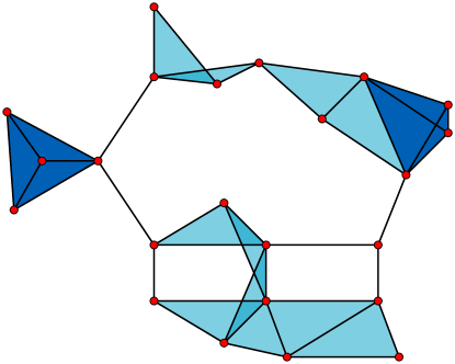
Figure 2.4: In this graph the maximal cliques are the two dark-blue colored subgraphs, each one of the 11 light blue colored triangles and all the edges that are not part of any of them [Eppstein 07].

In the case of the Ising model described in the beginning of this chapter, the underlying graph is the lattice and the maximal cliques are the edges that connect two neighbors. The probability of a configuration on the most general graphical model on a lattice is then

$$P(x_{1},...,x_{N})=\frac{1}{Z}\exp\left[\sum_{<i,j>}\log(p_{ij}(x_{i},x_{j}))\right]\,.$$ (2.38)

If we assume that our variables $x_{i}$ can take binary values $\pm 1$, the function $p_{ij}(x_{i},x_{j})$ is a function of $\{0,1\}\times\{0,1\}\rightarrow\mathbb{R}$, i. e., it can only take four different values: $p_{ij}(+1,+1)$, $p_{ij}(+1,-1)$, $p_{ij}(-1,+1)$ and $p_{ij}(-1,-1)$. There are an infinity of ways to express such a function with simple operations. We will choose the one that resembles the most with the Hamiltonian of a generalized Ising model:

$$\log(p_{ij}(x_{i},x_{j}))=J_{ij}\,x_{i}\,x_{j}+\tilde{h}_{ij}\,x_{i}+\tilde{h}_{ji}\,x_{j}+\kappa_{ij}\,.$$ (2.39)

Indeed, we can easily solve the linear system to find the four unknown values ($J_{ij}$, $\tilde{h}_{ij}$, $\tilde{h}_{ji}$ and $\kappa_{ij}$) as a function of the four different values of $p_{ij}(x_{i},x_{j})$.

Absorbing all the constants $\kappa_{ij}$ in the normalization $Z$ and posing $h_{i}=\sum_{j}\tilde{h}_{ij}$, our probability is

$$P(x_{1},...,x_{N})=\frac{1}{Z}\exp\left[\sum_{<i,j>}J_{ij}x_{i}x_{j}+\sum_{i}h_{i}x_{i}\right]\,,$$ (2.40)

which correspond to the probability of a Ising-like model with couplings between closest neighbors and where both the local fields and the coupling between the neighbors are site-dependent.

2.5.1 Message-passing algorithms

The expectation propagation is an interesting approximation for the general problem of evaluating averages according to a graphical model. The starting point of this method is the fact that when the underlying graph is a tree, we can evaluate these averages exactly. Suppose that we want to evaluate

$$P(x_{s})=\sum_{\{x_{1},...,x_{s-1},x_{s+1},...,x_{N}\}}P(x_{1},...,x_{N})\,.$$ (2.41)

We choose to represent our tree with $s$ as its root. In this case, we can write

$$P(x_{s})=\sum_{\{x_{1},...,x_{s-1},x_{s+1},...,x_{N}\}}\frac{1}{Z}\prod_{(r,s)\in E(G)}p_{r,s}(x_{r},x_{s})\,,$$ (2.42)

where $E(G)$ is the set of edges of the graph $G$. We can decompose this expression on each branches starting on $s$.

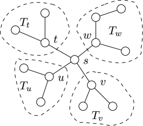
Figure 2.5: Example tree. Note the branches $T_{t},T_{u},T_{v}$ and $T_{w}$ starting on its root.

For the tree shown in Fig. 2.5, for example, it will be

$$\begin{split}P(x_{s})=\frac{1}{Z}&\left[\sum_{\{x_{r}\}_{r\in V(T_{t})}}p_{s,t}(x_{s},x_{t})\prod_{(r,d)\in E(T_{t})}p_{r,d}(x_{r},x_{d})\right]\times\\ \times&\left[\sum_{\{x_{r}\}_{r\in V(T_{u})}}p_{s,u}(x_{s},x_{u})\prod_{(r,d)\in E(T_{u})}p_{r,d}(x_{r},x_{d})\right]\times\\ \times&\left[\sum_{\{x_{r}\}_{r\in V(T_{v})}}p_{s,v}(x_{s},x_{v})\prod_{(r,d)\in E(T_{v})}p_{r,d}(x_{r},x_{d})\right]\times\\ \times&\left[\sum_{\{x_{r}\}_{r\in V(T_{w})}}p_{s,w}(x_{s},x_{w})\prod_{(r,d)\in E(T_{w})}p_{r,d}(x_{r},x_{d})\right]\end{split}$$ (2.43)

where each term in the product represents the contribution of one branch. As we can see, we transformed the Eq. (2.42) in four independent problems defined in each branch which can be solved separately. By repeating the procedure recursively, it is possible to solve the problem with a small number of operations. Note that the same divide-and-conquer method can be used also for evaluating $Z$.

We now would like to reformulate this solution as an algorithm that would also be well defined in graphs with cycles, even if not to give an exact solution nor being guaranteed to converge. The algorithm work by passing in each iteration messages $M_{st}$ from every two vertex $s$ and $t$ connected by an edge, corresponding to an iterative relation

$$M_{tr}(x_{r})\leftarrow\kappa\sum_{x_{t}^{\prime}}\left[p_{rt}(x_{r},x_{t}^{\prime})\prod_{u\in N(t),u\neq r}M_{ut}(x_{t}^{\prime})\right]\,,$$ (2.44)

where $N(t)$ is the set of neighbors of $t$ and $\kappa$ is a normalization constant fixing $\sum_{x_{r}}\prod_{t\in N(r)}M_{tr}(x_{r})=1$.

We can recover $P(x_{s})$ with the formula

$$P(x_{s})=\kappa\prod_{t\in N(s)}M_{ts}(x_{s})\,.$$ (2.45)

Note that the fixed point of this algorithm is the solution of (2.43). This algorithm is the simplest message-passing algorithm and is known as belief propagation. Several variations of this algorithm can be found in the literature[Wainwright 08].

Chapter 3 Inverse Problems

As exemplified in the previous chapters, most of the problems in statistical mechanics consist of describing the collective behavior of a large number of interacting parts. In general, the individual behavior of parts and how they interact are either described by first principles or can be very accurately measured. Unfortunately, as we have seen in chapter 1, for a few problems like neuron networks, the behavior of the parts and/or how they interact is not known, even if we can measure their collective behavior. In these cases, we would like to deduce the behavior and interactions of the parts from the available data. We talk then of inverse problems.

Inverse problems are often ill posed, i.e., there is more than one possible set of laws or parameters that can describe the observed data. To give an example, suppose all we know about a real-valued random variable $x$ is that $\left\langle x\right\rangle=0$ and $\left\langle x^{2}\right\rangle=1$. Even if we restrain ourselves to Bernoulli distributions, there is an infinity of distributions satisfying our conditions: for any real $a$, $P(x=a)=1/(1+a^{2})$ and $P(x=-1/a)=1-1/(1+a^{2})$ meet our requirements.

Intuitively, a possible criterion for choosing one among all these distributions is to look for the least “restrictive” one, i. e., the one which allows as many different values as possible. To formalize this criterion, we need to define the Shannon entropy of a statistical distribution. We will start thus this chapter by defining this entropy and presenting how to optimize it to put inverse problems in a well-defined framework. In the sequence, we will present the Bayesian inference, which is a complementary approach to the entropy optimization. Finally, we will define and present some known results for the inverse problem of most interest for this work: the inverse Ising problem.

3.1 Maximal entropy distribution

The Shannon entropy of a random variable is a measure of the quantity of information unknown about it. It is defined by the sum

$$S=-\sum_{\Omega}P(\Omega)\log P(\Omega)\,,$$ (3.1)

where $P(\Omega)$ is the probability of the configuration $\Omega$ of the system. Its interpretation as the quantity of information comes from the Shannon’s source coding theorem, which states that the best theoretically possible compression algorithm can encode a sampling of $N$ values taken with the distribution $P$ using $NS$ bits in the $N\rightarrow\infty$ limit.

If we are looking for the most general distribution that reproduces a set of averages $f_{i}=\left\langle f_{i}(X)\right\rangle$, it is reasonable to look for the one that maximizes $S$. This is known as the principle of maximum entropy. It can be interpreted as the model that satisfies our constraints, i. e., reproducing the prescribed set of averages, while imposing as few extra conditions as possible.

Let us now consider the interesting case of random binary variables $\sigma_{i}=\pm 1$, constraint to satisfy a set of local averages $\left\langle\sigma_{i}\right\rangle=m_{i}$ and correlations $\left\langle\sigma_{i}\sigma_{j}\right\rangle=C_{ij}$[Tkacik 06]. In principle, one could also consider imposing higher order correlations, like the three-site ones $C_{ijk}=\left\langle\sigma_{i}\sigma_{j}\sigma_{k}\right\rangle$, but doing so would only be useful in situations where one knows such high-order couplings precisely. Unfortunately, to extract such data from an experimental system one needs to measure a very large number of configurations of the system, which is rarely possible. We choose then to deal with only one and two-site correlations. In this case, we define generically the probability $P(\{\sigma_{i}\})=p_{\sigma_{1},...,\sigma_{N}}$ of a configuration $\{\sigma_{1},\ldots,\sigma_{N}\}$ and we can write the entropy as

$$S=-\sum_{\{\sigma\}}p_{\sigma_{1},...,\sigma_{N}}\log p_{\sigma_{1},...,\sigma_{N}}\,.$$ (3.2)

In order to impose the constraints on the averages and correlations, we add the Lagrange multipliers $h_{i}$, $J_{ij}$ and $\lambda$ respectively associated to $m_{i}=\langle\sigma_{i}\rangle$, $C_{ij}=\langle\sigma_{i}\sigma_{j}\rangle$ and to the normalization of the probability $\sum_{\{\sigma\}}p_{\sigma_{1},...,\sigma_{N}}=1$. We obtain

$$\begin{split}S=&-\sum_{\{\sigma\}}p_{\sigma_{1},...,\sigma_{N}}\log p_{\sigma_{1},...,\sigma_{N}}+\sum_{i}h_{i}\left(m_{i}-\sum_{\{\sigma\}}p_{\sigma_{1},...,\sigma_{N}}\sigma_{i}\right)\\ &+\sum_{i,j}J_{ij}\left(C_{ij}-\sum_{\{\sigma\}}p_{\sigma_{1},...,\sigma_{N}}\sigma_{i}\sigma_{j}\right)+\lambda\left(\sum_{\{\sigma\}}p_{\sigma_{1},...,\sigma_{N}}-1\right)\,.\end{split}$$ (3.3)

Optimizing $S$ on $p_{\sigma_{1},...,\sigma_{N}}$ we obtain

$$0=\lambda-1-\log p_{\sigma_{1},...,\sigma_{N}}+\sum_{i}h_{i}\sigma_{i}+\sum_{ij}J_{ij}\sigma_{i}\sigma_{j}\,.$$ (3.4)

Solving Eq. (3.4), we derive the probability distribution

$$P(\{\sigma\})=e^{\lambda-1}\exp\left(\sum_{ij}J_{ij}\sigma_{i}\sigma_{j}+\sum_{i}h_{i}\sigma_{i}\right)\,,$$ (3.5)

which corresponds exactly to the Boltzmann distribution for the generalized Ising model we presented in the beginning of chapter 2 (Eqs. (2.2) and (2.9)) for $\lambda-1=-\log Z$.

At this point, we know how the probability distribution depends on $J_{ij}$ and on $h_{i}$. To solve completely this problem, we need to express $J_{ij}$ and $h_{i}$ in terms of the imposed averages and correlations. Since $J_{ij}$ and $h_{i}$ are Lagrange multipliers, the values they should take to reproduce our averages and correlations correspond to an extrema of the entropy. To know whether it is a maximum or a minimum, we can do an explicit calculation of $\frac{\partial S}{\partial J_{ij}}$ and $\frac{\partial S}{\partial h_{i}}$ to see that the entropy is a convex function of the parameters $J_{ij}$ and $h_{i}$. Thus, we need to look for the set of parameters that minimizes the entropy. Moreover, the convexity assures that if a minimum exists, it is unique.

To illustrate, let’s examine the case of a two-spin system with $\left\langle\sigma_{1}\right\rangle=m_{1}$, $\left\langle\sigma_{2}\right\rangle=m_{2}$ and $\left\langle\sigma_{1}\sigma_{2}\right\rangle=C$. The entropy is given by

$$S = \log\left\{\sum_{\sigma_{1=\pm 1}}\sum_{\sigma_{2}=\pm 1}\exp\left[J\sigma_{1}\sigma_{2}+h_{1}\sigma_{1}+h_{2}\sigma_{2}\right]\right\}-JC-h_{1}m_{1}-h_{2}m_{2}\,,$$ (3.6)

$$= \log\left\{e^{J+h_{1}+h_{2}}+e^{J-h_{1}-h_{2}}+e^{-J+h_{1}-h_{2}}+e^{-J-h_{1}+h_{2}}\right\}$$

$$-JC-h_{1}m_{1}-h_{2}m_{2}\,.$$

Since we have only two spins, the optimization of $S$ with respect to $h_{1}$, $h_{2}$ and $J$ can be done explicitly and we obtain

$$J = \frac{1}{4}\log\left[\frac{(1+C-m_{1}-m_{2})(1+C+m_{1}+m_{2})}{(1-C-m_{1}+m_{2})(1-C+m_{1}-m_{2})}\right]$$ (3.7)

$$h_{1} = \frac{1}{4}\log\left[\frac{(1-C+m_{1}-m_{2})(1+C+m_{1}+m_{2})}{(1+C-m_{1}-m_{2})(1-C-m_{1}+m_{2})}\right]$$ (3.8)

$$h_{2} = \frac{1}{4}\log\left[\frac{(1-C-m_{1}+m_{2})(1+C+m_{1}+m_{2})}{(1+C-m_{1}-m_{2})(1-C+m_{1}-m_{2})}\right]\,.$$ (3.9)

3.2 Bayesian inference

Suppose now that we are not only interested in finding the best parameters to fit some data, but also in attributing a probability distribution to the set of these possible parameters. If our model depends on a set of unknown parameters $\{\lambda_{i}\}$ we could in principle write the probability $P(\{X_{i}\}|\{\lambda_{i}\})$ of measuring any set of configurations $\{X_{i}\}$. The Bayes theorem states that the probability of a set of parameters $\{\lambda_{i}\}$ as a function of a set of measures $\{X_{i}\}$ is

$$P(\{\lambda_{i}\}|\{X_{i}\})=\frac{P(\{X_{i}\}|\{\lambda_{i}\})P_{0}(\{\lambda_{i}\})}{P(\{X_{i}\})}\,,$$ (3.10)

where $P_{0}(\{\lambda_{i}\})$ is the a priori probability of the parameters $\{\lambda_{i}\}$ and $P(\{X_{i}\})$ is the marginal probability of $\{X_{i}\}$, which can also be interpreted as a normalization constant:

$$P(\{X_{i}\})=\sum_{\{\lambda_{i}\}}P(\{X_{i}\}|\{\lambda_{i}\})P_{0}(\{\lambda_{i}\})\,.$$ (3.11)

If one is looking to the set of parameters $\{\lambda_{i}\}$ that best describes the measures $\{X_{i}\}$, a natural choice is the one that maximizes Eq. (3.10). Such choice is known as the maximum a posteriori (MAP) estimator.

On the other hand, when the prior is not known, a common procedure is to look for the set of $\{\lambda_{i}\}$ that maximizes $P(\{X_{i}\}|\{\lambda_{i}\})$, which is the same as setting the prior to $P_{0}(\{\lambda_{i}\})=1$. We call such procedure the maximum likelihood estimation.

To illustrate, suppose that we have a coin that we know is biased in the following way: $P(\text{favored side})=1/2+\epsilon$ and $P(\text{unfavored side})=1/2-\epsilon$, but we do not know if head or tails is favored. We toss this coin three times and get three heads. Using the Bayes theorem, we have

$$P(\text{tails is favored}|\text{3 heads})=\frac{P(\text{3 heads}|\text{tails favored})P_{0}(\text{tails favored})}{P(\text{3 heads})}\,.$$ (3.12)

Since we have no prior knowledge whether head or tails is favored, we have $P_{0}(\text{tails favored})=P_{0}(\text{heads favored})=1/2$, which leads to

$$P(\text{tails are favored}|\text{3 heads}) = \frac{\left(\frac{1}{2}-\epsilon\right)^{3}}{\left(\frac{1}{2}-\epsilon\right)^{3}+\left(\frac{1}{2}+\epsilon\right)^{3}}\,,$$ (3.13)

and

$$P(\text{heads are favored}|\text{3 heads}) = \frac{\left(\frac{1}{2}+\epsilon\right)^{3}}{\left(\frac{1}{2}-\epsilon\right)^{3}+\left(\frac{1}{2}+\epsilon\right)^{3}}\,.$$ (3.14)

Unsurprisingly, we conclude that it is more likely that the coin’s favored side is heads.

Let us now look at a slightly different situation where the bias $\epsilon$ is unknown. As before, there is an unknown favored side and heads are obtained three times. We would like to determine $\epsilon$. From Eq. (3.10), we obtain an expression similar to Eq. (3.12)

$$P(\epsilon|\text{3 heads}) = \frac{\left(\frac{1}{2}+\epsilon\right)^{3}P_{0}(\epsilon)}{\int_{-1/2}^{1/2}\left(\frac{1}{2}+\epsilon^{\prime}\right)^{3}P_{0}(\epsilon^{\prime})\mathrm{\;d}\epsilon^{\prime}}\,.$$ (3.15)

Remark in the denominator the normalization according to Eq. (3.11). In this case the probability has a strong dependence on the prior, which is unknown in the majority of inference problems. Fortunately, this problem gets less and less important when one increases the amount of data. For example, suppose that instead of doing just three coin tosses, we toss it a large number of times, getting $N$ heads and $M$ tails. In this case, Eq. (3.15) becomes

$$P(\epsilon|\text{$N$ heads, $M$ tails}) = \frac{\left(\frac{1}{2}+\epsilon\right)^{N}\left(\frac{1}{2}-\epsilon\right)^{M}P_{0}(\epsilon)}{\int_{-1/2}^{1/2}\left(\frac{1}{2}+\epsilon^{\prime}\right)^{N}\left(\frac{1}{2}-\epsilon^{\prime}\right)^{M}P_{0}(\epsilon^{\prime})\mathrm{\;d}\epsilon^{\prime}}\,,$$ (3.16)

where the binomial term $\left(\begin{array}[]{c}N+M\\ N\end{array}\right)$ gets canceled out with the normalization. Since the function $\left(\frac{1}{2}+\epsilon\right)^{N}\left(\frac{1}{2}-\epsilon\right)^{M}$ has a very sharp peak around $(N-M)/(2M+2N)$, we can do the following approximation:

$$\left(\frac{1}{2}+\epsilon\right)^{N}\left(\frac{1}{2}-\epsilon\right)^{M}P_{0}(\epsilon)\,\simeq\,\left(\frac{1}{2}+\epsilon\right)^{N}\left(\frac{1}{2}-\epsilon\right)^{M}P_{0}\left(\frac{N-M}{2M+2N}\right)\,.$$ (3.17)

If we apply this approximation to Eq. (3.15), the value $P_{0}\left(\frac{N-M}{2M+2N}\right)$ appears both in the numerator and in the denominator and will cancel out. The probability is thus independent of the unknown function $P_{0}(\epsilon)$.

In other situations, the prior might be useful to make an inference procedure more robust. Suppose for example that we are measuring a system composed by a large number of spins $\{\sigma_{i}\}$. By pure coincidence (or lack of data), two particular sites, $i$ and $j$, have identical spin values in all the measured configurations. Without defining a prior (i.e, setting $P_{0}(\alpha)=1$), the algorithm will infer an infinite-valued coupling between the two sites to account for this, which is non-physical and numerically problematic. On the other hand, if we suppose that $P_{0}(\alpha)$ is a Gaussian distribution, the prior will skew the inferred values away from very large values, avoiding the problematic solutions.

3.2.1 Relationship with entropy maximization

Suppose that we make $L$ independent measurements $\{\sigma_{l}\}$ of a system we would like to describe using a set of parameters $\alpha$. Since the measures are independent, we can write

$$\log P(\{\sigma\}|\alpha)=\sum_{l=1}^{L}\log P(\sigma_{l}|\alpha)\,.$$ (3.18)

Using the maximum a posteriori principle and the Bayes theorem, the set of $\alpha$ that best describes the data is

$$\alpha=\mathop{\text{argmax}}_{\alpha^{\prime}}\left[\log P_{0}(\alpha^{\prime})+\sum_{l=1}^{L}\log P(\sigma_{l}|\alpha^{\prime})\right]\,,$$ (3.19)

where $P_{0}(\alpha)$ is the prior probability of $\alpha$. If we want to use the principle of the maximization of the entropy, one should estimate the entropy from the data as

$$S(\alpha)=-\frac{1}{L}\sum_{l=1}^{L}\log P(\sigma_{l}|\alpha)\,\simeq-\left\langle\log P(\sigma|\alpha)\right\rangle_{\sigma}\,,$$ (3.20)

using the definition of an average, we can show that $S(\alpha)$ corresponds to the usual definition of the entropy

$$S(\alpha)\,\simeq\,-\sum_{\{\sigma\}}P(\sigma|\alpha)\log P(\sigma|\alpha)\,.$$ (3.21)

As we saw in the last section, we should then minimize $S(\alpha)$ with respect to the parameters $\alpha$, what corresponds exactly to maximizing $P(\{\sigma\}|\alpha)$, as one would do using the maximum likelihood method.

3.3 The inverse Ising problem: some results from the literature

We call the problem of finding the set of couplings $\{J_{ij}\}$ and local fields $\{h_{i}\}$ from the set of magnetizations $\{m_{i}\}$ and correlations $\{C_{ij}\}$ of a generalized Ising model the inverse generalized Ising problem [Schneidman 06]. In the following, we will omit the mention “generalized” for simplicity. We expect this problem to be particularly hard, since as we have seen in chapter 2, the direct problem of finding the magnetizations from the model’s parameters is already a non-trivial one.

3.3.1 Monte Carlo optimization

One can use the fact that the direct problem is numerically solvable with Monte Carlo (MC) methods [Krauth 06] to solve the inverse problem with the following algorithm [Ackley 85]:

1. start with an initial guess for the parameters $J_{ij}^{0}$ and $h_{i}^{0}$.

2. do a Monte-Carlo simulation to find the set of magnetization $m_{i}^{\text{est}}$ and correlations $C_{ij}^{\text{est}}$ corresponding to these parameters.

3. update $J_{ij}$ according to $J_{ij}^{t+1}=J_{ij}^{t}+\eta(t)(C_{ij}-C_{ij}^{\text{est}})+\alpha(J_{ij}^{t}-J_{ij}^{t-1})$ for some chosen function $\eta$ and constant $\alpha$.

4. update $h_{i}$ analogously to $J_{ij}$.

5. repeat steps 2 – 4 until $\max_{ij}(C_{ij}-C_{ij}^{\text{est}})<\epsilon$.

The number of steps necessary to reach a certain accuracy depends both on the initial parameters, the function $\eta$ and the parameter $\alpha$. An important drawback of this algorithm is that it is very inefficient: at each step one must do a Monte-Carlo simulation that is very time-consuming if one needs an accurate result. There are others modified versions of this algorithm that improve the number of necessary steps [Broderick 07], but they all involve doing a MC simulation at every step and thus have the same drawbacks.

3.3.2 Susceptibility propagation

In 2008, M. Mézard and T. Mora had the interesting idea of modifying the message passing algorithm we have seen in section 2.5.1 to solve the inverse Ising problem [Mezard 08, Marinari 10].

In their paper, the authors first write the Belief Propagation equations to find the values of $C_{ij}$ and $m_{i}$. They reinterpret these equations by identifying $\{J_{ij},h_{i}\}$ as the unknowns and $\{C_{ij},m_{i}\}$ as the input data and describe a message passing procedure that converges to the right fixed-point in trees. The details can be found in [Marinari 10].

This procedure, in the same way as the belief propagation for the direct problem, is exact on trees and an approximation for graphs that contain loops. If it converges (which is not guaranteed in graphs with loops), it do so in polynomial time, which makes it much faster than the Monte Carlo optimization. The main drawback of this method is that for graphs with loops the resulting approximated solution might be very far from the optimal solution of the problem.

3.3.3 Inversion of TAP equations

Another approach for solving the inverse Ising problem was proposed by Roudi et al.[Roudi 09]. Their starting point are the TAP equations we already saw in section 2.3:

$$\tanh^{-1}m_{i}=h_{i}+\sum_{j\,(\neq i)}J_{ij}m_{j}-m_{i}\sum_{j\,(\neq i)}J_{ij}^{2}(1-m_{j}^{2})\,.$$ (3.22)

Taking the derivative of this expression with respect to $m_{j}$ and noting that $(C^{-1})_{ij}=\partial h_{i}/\partial m_{j}$, we have

$$(C^{-1})_{ij}=-J_{ij}-2J_{ij}^{2}m_{i}m_{j}+(1-m_{i}^{2})^{-1}\delta_{ij}\,,$$ (3.23)

which is easily solvable for $J_{ij}$.

Note that if $J_{ij}$ is small, we can neglect the $J_{ij}^{2}$ term, yielding an explicit solution for the couplings

$$J_{ij}=(C^{-1})_{ij}-(1-m_{i}^{2})^{-1}\delta_{ij}\,.$$ (3.24)

The inversion of Eq. (3.23) has the same strengths and drawbacks of the use of the TAP equations in the direct problem: it is exact in the large size limit for the SK model and we might expect it to work well only in models where the couplings are small.

3.3.4 Auto-consistent equations

Recently, a novel approach for finding the parameters of an Ising model was proposed by the statistics community[Wainwright 10]. Its main idea reposes on the fact that for a Ising system, the magnetization respects

$$m_{i} = \sum_{\{\sigma_{k}\}_{k\neq i}}\sum_{\sigma_{i}=\pm 1}\sigma_{i}\exp\left[\sigma_{i}\sum_{k}J_{ij}\sigma_{j}+\mathop{\sum_{j<k}}_{j\neq i\neq k}J_{jk}\sigma_{j}\sigma_{k}+\sum_{j}h_{j}\sigma_{j}+h_{i}\sigma_{i}\right]$$ (3.25)

$$= \left\langle\tanh\left(\sum_{j\,(\neq i)}J_{ij}\sigma_{j}+h_{i}\right)\right\rangle\,,$$

where we used the fact that $\sum_{\sigma=\pm 1}\sigma e^{\sigma A}=\tanh(A)\sum_{\sigma=\pm 1}e^{\sigma A}$. An analogous expression can be derived for the correlations:

$$C_{ij}=\left\langle\frac{{A_{ij}(\sigma,+,+)}-{A_{ij}(\sigma,+,-)}-{A_{ij}(\sigma,-,+)}+{A_{ij}(\sigma,-,-)}}{{A_{ij}(\sigma,+,+)}+{A_{ij}(\sigma,+,-)}+{A_{ij}(\sigma,-,+)}+{A_{ij}(\sigma,-,-)}}\right\rangle\,,$$ (3.26)

where

$$A_{ij}(\sigma,\tau,\rho)=\exp\left[\rho\tau J_{ij}+\rho\sum_{k}J_{ik}\sigma_{k}+\tau\sum_{k}J_{jk}\sigma_{k}+\tau h_{i}+\rho h_{j}\right]\,.$$ (3.27)

Suppose now that we have a set of $L$ independent measures of the full spin configuration of our system $\{\sigma^{1},...,\sigma^{L}\}$, with $\sigma^{k}=\{\sigma^{k}_{1},...\sigma^{k}_{N}\}$. We can then estimate Eqs. (3.25) and (3.26):

$$\frac{1}{L}\sum_{l=1}^{L}\sigma_{i}^{l}=\frac{1}{L}\sum_{l=1}^{L}\tanh\left(\sum_{j\,(\neq i)}J_{ij}\sigma_{j}^{l}+h_{i}\right)\,,$$ (3.28)

and, respectively,

$$\begin{split}\frac{1}{L}\sum_{l=1}^{L}\sigma_{i}^{l}\sigma_{j}^{l}=&\\ =\frac{1}{L}\sum_{l=1}^{L}&\frac{{A_{ij}(\sigma^{l},+,+)}-{A_{ij}(\sigma^{l},+,-)}-{A_{ij}(\sigma^{l},-,+)}+{A_{ij}(\sigma^{l},-,-)}}{{A_{ij}(\sigma^{l},+,+)}+{A_{ij}(\sigma^{l},+,-)}+{A_{ij}(\sigma^{l},-,+)}+{A_{ij}(\sigma^{l},-,-)}}\,.\end{split}$$ (3.29)

We have thus a system of coupled non-linear equations for $J_{ij}$ and $h_{i}$ which can be solved without the need to evaluate the partition function $Z$.

This procedure allows one to find the couplings from the measured data in polynomial time, but it has a few drawbacks. First of all, this procedure is not optimal according to the Bayes theorem. It depends on all high-order correlations while the optimal Bayes inference depends only on magnetizations and correlations. Accordingly, this method does not work if the Hamiltonian used to generate the data has any three or higher order couplings. This is particularly awkward for the case of inferring neural synapses where the hypothesis of the Ising model is just an approximation. Finally, solving the set of equations for $J_{ij}$ is a non-trivial problem. The original paper[Wainwright 10] proposes an algorithm to solve it that unfortunately does not work in the low-temperature regime.

Part II Some results on the inverse Ising problem

Chapter 4 The inverse Ising problem in the small-correlation limit

In section 3.3, we have introduced the inverse Ising problem and discussed what has been done in the literature to solve it. In this chapter, we propose a small-correlation expansion procedure that allows one to find the couplings and magnetizations up to any given power on the correlations[Sessak 09]. We will find an explicit expression for the couplings and magnetizations that is correct up to $O((\text{largest connected correlation})^{3})$.

We consider the generalized Ising model for a system composed of $N$ spins $\sigma_{i}=\pm 1$, $i=1,\ldots,N$, whose Hamiltonian is given by

$$H(\{\sigma_{i}\})=-\sum_{i<j}J_{ij}\,\sigma_{i}\,\sigma_{j}-\sum_{i}h_{i}\,\sigma_{i}\,,$$ (4.1)

as we have already introduced in chap. 2, in Eq. (2.9). We want to find the values of couplings $J_{ij}^{*}$ and fields $h^{*}_{i}$ such that the average values of the spins and of the spin-spin correlations match the prescribed magnetizations $m_{i}$, given by

$$m_{i}=\left\langle\sigma_{i}\right\rangle\,,$$ (4.2)

and connected correlations $c_{ij}$, defined by

$$c_{ij}=\left\langle\sigma_{i}\sigma_{j}\right\rangle-m_{i}\;m_{j}\,.$$ (4.3)

For given fixed magnetizations and correlations, the entropy of the generalized Ising model, obtained in section 3.1, is given by

$$S(\{J_{ij}\},\{\lambda_{i}\};\{m_{i}\},\{c_{ij}\})=\log Z(\{J_{ij}\},\{h_{i}\})-\sum_{i<j}J_{ij}\,(c_{ij}+m_{i}\,m_{j})-\sum_{i}h_{i}\,m_{i}\,,\\$$

$$\begin{split}\phantom{xxxx}&=\log\sum_{\{\sigma_{i}\}}\exp\left\{\sum_{i<j}J_{ij}\left[\sigma_{i}\sigma_{j}-c_{ij}-m_{i}m_{j}\right]+\sum_{i}h_{i}(\sigma_{i}-m_{i})\right\}\,,\\ &=\log\sum_{\{\sigma_{i}\}}\exp\left\{\sum_{i<j}J_{ij}\left[(\sigma_{i}-m_{i})(\sigma_{j}-m_{j})-c_{ij}\right]+\sum_{i}\lambda_{i}(\sigma_{i}-m_{i})\right\}\,,\end{split}$$ (4.4)

where the new fields $\lambda_{i}$ are simply related to the physical fields $h_{i}$ through $\lambda_{i}=h_{i}+\sum_{j}J_{ij}\,m_{j}$. In this same section, we have seen that the couplings $J_{ij}^{*}$ and fields $h_{i}^{*}$ are the ones that minimize the entropy. As discussed in chap. 2, the exact evaluation of the entropy shown in Eq. (4.4) for a given set of $J_{ij}$ and $\lambda_{i}$ is, in general, a computationally challenging task, not to say about its minimization. To obtain a tractable expression we multiply all connected correlations $c_{ij}$ in Eq. (4.4) by the same small parameter $\beta$, which can be interpreted as a fictitious inverse temperature. Our entropy is thus

$$S(\{J_{ij}\},\{\lambda_{i}\};\{m_{i}\},\{\beta\,c_{ij}\})=\\ =\log\sum_{\{\sigma_{i}\}}\exp\left\{\sum_{i<j}J_{ij}\left[(\sigma_{i}-m_{i})(\sigma_{j}-m_{j})-\beta c_{ij}\right]+\sum_{i}\lambda_{i}(\sigma_{i}-m_{i})\right\}\,,$$ (4.5)

In this chapter we want to expand the entropy in powers of $\beta$ as a function of the magnetizations and correlations:

$$S(\{m_{i}\},\{\beta\,c_{ij}\})=S^{0}+\beta S^{1}+\beta^{2}S^{2}+\ldots\,,$$ (4.6)

Accordingly, $J_{ij}^{*}$ and $\lambda_{i}^{*}$ can also be written as series on $\beta$:

$$J_{ij}^{*}(\{m_{i}\},\{\beta\,c_{ij}\}) = J_{ij}^{0}+\beta J_{ij}^{1}+\beta^{2}J_{ij}^{2}+\ldots\,,$$ (4.7)

$$\lambda_{i}^{*}(\{m_{i}\},\{\beta\,c_{ij}\}) = \lambda_{i}^{0}+\beta\lambda_{i}^{1}+\beta^{2}\lambda_{i}^{2}+\ldots\,,$$ (4.8)

where we omit the dependency of the terms on $\{m_{i}\}$ and $\{c_{ij}\}$ to make notations lighter. The entropy we are looking for will be obtained when setting $\beta=1$ in the expansion. Since the parameter $\beta$ multiply every value of $c_{ij}$, we have that $S^{k}=O(c_{ij}^{k})$. We can thus deduce that our expansion for $S$ will be convergent for small enough couplings. Note that once we have expressed the entropy as a series on $\beta$, we can retrieve an expansion for couplings and fields using the following identities, that follow from the definition of the entropy:

$$\frac{\partial S(\{m_{i}\},\{\beta\;c_{ij}\})}{\partial c_{ij}}=-\beta J_{ij}^{*}(\beta)\,,$$ (4.9)

and

$$\frac{\partial S(\{m_{i}\},\{\beta\;c_{ij}\})}{\partial m_{i}}=-\lambda_{i}^{*}(\beta)\,.$$ (4.10)

Thus, once we have found an expansion for $S$, it is trivial to deduce from it an expansion for $J_{ij}^{*}$ and $\lambda_{i}^{*}$.

The calculation of the entropy $S(\{m_{i}\},\{\beta\,c_{ij}\})$ is straightforward for $\beta=0$ since spins are uncoupled in this limit. In this case, the values of the couplings and fields minimizing the entropy are thus

$$J^{0}_{ij}=0\qquad\text{and}\qquad\lambda^{0}_{i}=\tanh^{-1}(m_{i})\ .$$ (4.11)

Accordingly, the entropy for $\beta=0$ is

$$S^{0}=-\sum_{i}\left[\frac{1+m_{i}}{2}\ln\frac{1+m_{i}}{2}+\frac{1-m_{i}}{2}\ln\frac{1-m_{i}}{2}\right]\,.$$ (4.12)

To find the non-trivial terms of the entropy we proceed in the following way: first we define a potential $U$ over the spin configurations at inverse temperature $\beta$ through (note the new last term)

$$\begin{split}U(\{\sigma_{i}\})&=\sum_{i<j}J_{ij}^{*}(\beta)\left[(\sigma_{i}-m_{i})(\sigma_{j}-m_{j})-\beta\;c_{ij}\right]+\sum_{i}\lambda_{i}^{*}(\beta)(\sigma_{i}-m_{i})\\ &+\sum_{i<j}c_{ij}\int_{0}^{\beta}\mathrm{\;d}\beta^{\prime}J_{ij}^{*}(\beta^{\prime})\,,\end{split}$$ (4.13)

and a modified entropy (compare to Eq. (4.4))

$$\tilde{S}(\{m_{i}\},\{c_{ij}\},\beta)=\log\sum_{\{\sigma_{i}\}}e^{U(\{\sigma_{i}\})}\ .$$ (4.14)

Notice that $U$ depends on the coupling values $J^{*}_{ij}(\beta^{\prime})$ at all inverse temperatures $\beta^{\prime}<\beta$. The true entropy (at its minimum) and the modified entropy are simply related to each other through

$$S(\{m_{i}\},\{c_{ij}\},\beta)=\tilde{S}(\{m_{i}\},\{c_{ij}\},\beta)-\sum_{i<j}c_{ij}\int_{0}^{\beta}\mathrm{\;d}\beta^{\prime}J_{ij}^{*}(\beta^{\prime})\ .$$ (4.15)

The modified entropy $\tilde{S}$ in Eq. (4.14) was chosen to be independent of $\beta$. Indeed, it has an explicit dependence on $\beta$ through the potential $U$ (Eq. (4.13)), and an implicit dependence through the couplings and the fields. As the latter are chosen to minimize $S$, the full derivative of $\tilde{S}$ with respect to $\beta$ coincides with its partial derivative, and we get

$$\frac{d\tilde{S}}{d\beta}=\frac{\partial\tilde{S}}{\partial\beta}=-\sum_{i<j}c_{ij}\;J_{ij}^{*}(\beta)+\sum_{i<j}c_{ij}\;J_{ij}^{*}(\beta)=0\ .$$ (4.16)

The above equality is true for any $\beta$. Consequently, $\tilde{S}$ is constant and equal to its value at $\beta=0$, $S^{0}$, given in Eq. (4.12).

In the following, we will use the fact that $\tilde{S}$ does not depend on $\beta$ to write self-consistency equations from which we will deduce our expansion. We will start by presenting $S^{1}$ and $S^{2}$ since their calculations differ from those used for higher orders. Afterwards, we will present the calculations for $S^{3}$ as a generalizable example of the general method, which will be presented in the sequence.

4.1 Evaluation of S¹ and S²

To find $S^{1}$, we derive Eq. (4.15) with respect to $\beta$:

$$S^{1} = \left.\frac{\partial S}{\partial\beta}\right|_{0}=\left.\frac{\partial\tilde{S}}{\partial\beta}\right|_{0}-\sum_{i<j}c_{ij}J_{ij}^{*}(0)\,,$$ (4.17)

$$= 0\,,$$

since $\tilde{S}$ does not depend on $\beta$ (Eq. (4.16)) and $J_{ij}^{*}(0)=J_{ij}^{0}=0$ (Eq. (4.11)). A direct consequence of this, deriving from Eq. (4.10), is

$$\left.\frac{\partial\lambda_{i}}{\partial\beta}\right|_{0}=0=\lambda^{1}\,.$$ (4.18)

To evaluate the next term $S^{2}$, we note that since $\frac{\mathrm{\;d}\tilde{S}(\beta)}{\mathrm{\;d}\beta}=0$ for any $\beta$, we have in particular that

$$\frac{\partial\tilde{S}}{\partial\beta}=0=\frac{1}{\sum_{\{\sigma\}}e^{U(\{\sigma\},\beta)}}\sum_{\{\sigma\}}\frac{\partial U(\{\sigma\})}{\partial\beta}e^{U(\{\sigma\})}=\left\langle\frac{\partial U}{\partial\beta}\right\rangle\,.$$ (4.19)

Evaluating Eq. (4.19) explicitly for $\beta=0$ yields

$$0=-\sum_{i<j}c_{ij}J_{ij}^{*}(0)+\sum_{i<j}\left.\frac{\partial J_{ij}^{*}}{\partial\beta}\right|_{0}\left\langle(\sigma_{i}-m_{i})(\sigma_{j}-m_{j})\right\rangle_{0}\,,$$ (4.20)

This equality is trivial, since we know that $J_{ij}^{*}(0)=0$ and the averages also vanish since the spins are uncoupled for $\beta=0$. We must thus look at the second derivative of $\tilde{S}$:

$$\frac{\partial^{2}\tilde{S}}{\partial\beta^{2}}=0=\left\langle\frac{\partial^{2}U}{\partial\beta^{2}}\right\rangle+\left\langle\left(\frac{\partial U}{\partial\beta}\right)^{2}\right\rangle-\left\langle\frac{\partial U}{\partial\beta}\right\rangle^{2}\,.$$ (4.21)

Explicitly, the first term corresponds to

$$\frac{\partial^{2}U}{\partial\beta^{2}} = \sum_{i<j}\frac{\partial^{2}J_{ij}^{*}}{\partial\beta^{2}}(\sigma_{i}-m_{i})(\sigma_{j}-m_{j})+\sum_{i}\frac{\partial^{2}\lambda_{i}^{*}}{\partial\beta^{2}}(\sigma_{i}-m_{i})$$ (4.22)

$$-\sum_{i<j}\frac{\partial J_{ij}^{*}}{\partial\beta}c_{ij}-\beta\sum_{i<j}\frac{\partial^{2}J_{ij}^{*}}{\partial\beta^{2}}c_{ij}\,,$$

which for $\beta=0$ yields

$$\left.\frac{\partial^{2}U}{\partial\beta^{2}}\right|_{0} = -\sum_{i<j}c_{ij}\left.\frac{\partial J_{ij}^{*}}{\partial\beta}\right|_{0}\,,$$ (4.23)

The next one is given by

$$\left.\left(\frac{\partial U}{\partial\beta}\right)^{2}\right|_{0} = \sum_{i<j}\sum_{k<l}\frac{\partial J_{ij}^{*}}{\partial\beta}\frac{\partial J_{kl}^{*}}{\partial\beta}\left(\sigma_{i}-m_{i}\right)\left(\sigma_{j}-m_{j}\right)\left(\sigma_{k}-m_{k}\right)\left(\sigma_{l}-m_{l}\right)$$ (4.24)

$$+\sum_{i,j}\frac{\partial\lambda_{i}^{*}}{\partial\beta}\frac{\partial\lambda_{j}^{*}}{\partial\beta}(\sigma_{i}-m_{i})(\sigma_{j}-m_{j})$$

$$+2\sum_{i<j}\sum_{k}\frac{\partial J_{ij}^{*}}{\partial\beta}\frac{\partial\lambda_{i}^{*}}{\partial\beta}(\sigma_{i}-m_{i})(\sigma_{j}-m_{j})(\sigma_{k}-m_{k})\,,$$

which for $\beta=0$ reduces to

$$\left\langle\left(\frac{\partial U}{\partial\beta}\right)^{2}\right\rangle_{0} = \sum_{i<j}\left(\left.\frac{\partial J_{ij}^{*}}{\partial\beta}\right|_{0}\right)^{2}(1-m_{i}^{2})(1-m_{j}^{2})\,,$$ (4.25)

where we used in the last equation the fact that $\left.\frac{\partial\lambda_{i}^{*}}{\partial\beta}\right|_{0}=\lambda_{i}^{1}=0$ (Eq. (4.18)). The last term vanishes as consequence of Eq. (4.19).

Finally, we can rewrite Eq. (4.21) as

$$\sum_{i<j}c_{ij}\left.\frac{\partial J_{ij}^{*}}{\partial\beta}\right|_{0}=\sum_{i<j}\left(\left.\frac{\partial J_{ij}^{*}}{\partial\beta}\right|_{0}\right)^{2}(1-m_{i}^{2})(1-m_{j}^{2})\,,$$ (4.26)

whose simpler solution is given by

$$\left.\frac{\partial J_{ij}^{*}}{\partial\beta}\right|_{0}=\frac{c_{ij}}{(1-m_{i}^{2})(1-m_{j}^{2})}=J_{ij}^{1}\,.$$ (4.27)

Using Eqs. (4.15) and (4.10) we can now deduce

$$S^{2}=-\frac{1}{2}\sum_{i<j}\frac{c_{ij}^{2}}{(1-m_{i}^{2})(1-m_{j}^{2})}\,,$$ (4.28)

and

$$\left.\frac{\partial^{2}\lambda_{i}^{*}}{\partial\beta^{2}}\right|_{0}=2m_{i}\sum_{j}\frac{c_{ij}^{2}}{(1-m_{i}^{2})(1-m_{j}^{2})^{2}}=2\lambda_{i}^{2}\,.$$ (4.29)

Finally, we have the value of $\lambda_{i}^{2}$, $S^{2}$ and our first non-trivial estimation of $J_{ij}^{*}$. We can verify the correctness of Eq. (4.27) by noting it is the first-order approximation of Eq. (3.7) for small $c$.

4.2 Evaluation of S³

Like in previous section, we calculate the third derivative of $\tilde{S}$ with respect to $\beta$:

$$0=\frac{\partial^{3}\tilde{S}}{\partial\beta^{3}}=\left\langle\frac{\partial^{3}U}{\partial\beta^{3}}\right\rangle+3\left\langle\frac{\partial^{2}U}{\partial\beta^{2}}\frac{\partial U}{\partial\beta}\right\rangle+\left\langle\left(\frac{\partial U}{\partial\beta}\right)^{3}\right\rangle\,,$$ (4.30)

which yields, after evaluating the averages (see appendix A):

$$\sum_{i<j}c_{ij}\left.\frac{\partial^{2}J_{ij}^{*}}{\partial\beta^{2}}\right|_{0}=-4\sum_{i<j}\frac{c_{ij}^{3}m_{i}m_{j}}{(1-m_{i}^{2})^{2}(1-m_{j}^{2})^{2}}-6\sum_{i<j<k}\frac{c_{ij}c_{jk}c_{ki}}{(1-m_{i}^{2})(1-m_{j}^{2})(1-m_{k}^{2})}\,.$$ (4.31)

Taking the third derivative of Eq. (4.15), we can show that

$$-\sum_{i<j}c_{ij}\left.\frac{\partial^{2}J_{ij}^{*}}{\partial\beta^{2}}\right|_{0}=\left.\frac{\partial^{3}S}{\partial\beta^{3}}\right|_{0}=6S^{3}\,.$$ (4.32)

Comparing the two last equations, we finally find the expression for $S^{3}$:

$$S^{3}=\frac{2}{3}\sum_{i<j}\frac{c_{ij}^{3}m_{i}m_{j}}{(1-m_{i}^{2})^{2}(1-m_{j}^{2})^{2}}+\sum_{i<j<k}\frac{c_{ij}c_{jk}c_{ki}}{(1-m_{i}^{2})(1-m_{j}^{2})(1-m_{k}^{2})}\,.$$ (4.33)

4.3 Higher orders

The expansion procedure can be continued order by order using the same procedure as in section 4.2. To evaluate $S^{k}$ having already evaluated all $S^{n}$ for $n<k$, one must evaluate $\left.\frac{\partial^{k}\tilde{S}}{\partial\beta^{k}}\right|_{0}$ as a sum of averages with respect to uncoupled spins. After evaluating explicitly the averages, one will have

$$\left.\frac{\partial^{k}\tilde{S}}{\partial\beta^{k}}\right|_{0}=-\sum_{i<j}c_{ij}\left.\frac{\partial^{k-1}J_{ij}^{*}}{\partial\beta^{k-1}}\right|_{0}+Q_{k}\,,$$ (4.34)

where $Q_{k}$ is a (known) function of the magnetizations, correlations, and of the derivatives in $\beta=0$ of the couplings $J_{ij}^{*}$ and fields $\lambda_{i}^{*}$ of order $\leq\max(1,k-2)$. See Appendices A and B.

Finally, as $\tilde{S}$ is constant by virtue of Eq. (4.16), both sides of Eq. (4.34) vanish. Using Eq. (4.15), we have

$$S^{k}=-\frac{Q_{k}}{k!}\,,$$ (4.35)

which allows then to find the fields and couplings using Eqs. (4.9-4.10).

Using this procedure, we could go up to $S^{4}$ (details are on Appendix A). Using the notations

$$L_{i}=\left\langle\left(\sigma_{i}-m_{i}\right)^{2}\right\rangle_{0}=1-m_{i}^{2}\,,$$ (4.36)

which is basically the variance of an independent spin of average $m_{i}$ and

$$K_{ij}=(1-\delta_{ij})\frac{\left\langle\left(\sigma_{i}-m_{i}\right)\left(\sigma_{j}-m_{j}\right)\right\rangle_{0}}{\left\langle\left(\sigma_{i}-m_{i}\right)^{2}\right\rangle_{0}\left\langle\left(\sigma_{j}-m_{j}\right)^{2}\right\rangle_{0}}=(1-\delta_{ij})\frac{c_{ij}}{L_{i}L_{j}}\,,$$ (4.37)

where we have multiplied our definition of $K_{ij}$ by one minus a Kronecker symbol so that $K_{ii}=0$, what makes our notations simpler. With these definitions, we have

$$S = -\sum_{i}\left[\frac{1+m_{i}}{2}\ln\frac{1+m_{i}}{2}+\frac{1-m_{i}}{2}\ln\frac{1-m_{i}}{2}\right]$$ (4.38)

$$-\frac{\beta^{2}}{2}\sum_{i<j}K_{ij}^{2}L_{i}L_{j}+\frac{2}{3}\beta^{3}\sum_{i<j}K_{ij}^{3}m_{i}m_{j}L_{i}L_{j}+\beta^{3}\sum_{i<j<k}K_{ij}K_{jk}K_{ki}L_{i}L_{j}L_{k}$$

$$-\frac{\beta^{4}}{12}\sum_{i<j}K_{ij}^{4}\left[1+3m_{i}^{2}+3m_{j}^{2}+9m_{i}^{2}m_{j}^{2}\right]L_{i}L_{j}-\frac{\beta^{4}}{2}\sum_{i<j}\sum_{k}K_{ik}^{2}K_{kj}^{2}L_{k}^{2}L_{i}L_{j}$$

$$-\beta^{4}\sum_{i<j<k<l}(K_{ij}K_{jk}K_{kl}K_{li}+K_{ik}K_{kj}K_{lj}K_{il}+K_{ij}K_{jl}K_{lk}K_{ki})L_{i}L_{j}L_{k}L_{l}$$

$$+O(\beta^{5})\,.$$

The result for $J_{ij}^{*}$ is

$$J_{ij}^{*}(\{c_{kl}\},\{m_{i}\},\beta) = \beta K_{ij}-2\beta^{2}m_{i}m_{j}K_{ij}^{2}-\beta^{2}\sum_{k}K_{jk}K_{ki}L_{k}$$ (4.39)

$$+\frac{1}{3}\beta^{3}K_{ij}^{3}\left[1+3m_{i}^{2}+3m_{j}^{2}+9m_{i}^{2}m_{j}^{2}\right]$$

$$+\beta^{3}\sum_{\begin{subarray}{c}k\\ (\neq i,\,\neq j)\end{subarray}}K_{ij}(K_{jk}^{2}L_{j}+K_{ki}^{2}L_{i})L_{k}$$

$$+\beta^{3}\sum_{\begin{subarray}{c}k,l\\ (k\neq i,\,l\neq j)\end{subarray}}K_{jk}K_{kl}K_{li}L_{k}L_{l}+O(\beta^{4})\,,$$

and the physical field is given by

$$h_{l}^{*}(\{c_{ij}\},\{m_{i}\},\beta) = \frac{1}{2}\ln\left(\frac{1+m_{l}}{1-m_{l}}\right)-\sum_{j}J_{lj}^{*}m_{j}+\beta^{2}\sum_{j(\neq l)}K_{lj}^{2}m_{l}L_{j}$$ (4.40)

$$-\frac{2}{3}\beta^{3}(1+3m_{l}^{2})\sum_{j(\neq l)}K_{lj}^{3}m_{j}L_{j}-2\beta^{3}m_{l}\sum_{j<k}K_{lj}K_{jk}K_{kl}L_{j}L_{k}$$

$$+2\beta^{4}m_{l}\sum_{i<j}\sum_{k}K_{ik}K_{kj}K_{jl}K_{li}L_{i}L_{j}L_{k}$$

$$+\beta^{4}m_{l}\sum_{j}K_{lj}^{4}L_{j}\left[1+m_{l}^{2}+3m_{j}^{2}+3m_{l}^{2}m_{j}^{2}\right]$$

$$+\beta^{4}m_{l}\sum_{i\,(\neq l)}\sum_{j}K_{ij}^{2}K_{jl}^{2}L_{i}L_{j}^{2}+O(\beta^{5})\,.$$

4.4 Checking the correctness of the expansion

As we can see in Appendix A, the calculations for getting to Eq. (4.38) are long and error-prone. In this section, we will look at the different methods used to verify the correctness of these calculations.

4.4.1 Comparing the values of the external field with TAP equations

In section 2.3, we presented an expansion of the free energy of the direct Ising model for small couplings. The first two orders were developed by Thouless et al. to solve the SK model, and are given in Eq. (2.30). In 1991 A. Georges and J. Yedidia [Georges 91] published the next two orders of this expansion. They found

$$-\beta F(\{\beta J_{ij}\},\{m_{i}\}) = -\sum_{i}\left[\frac{1+m_{i}}{2}\ln\frac{1+m_{i}}{2}+\frac{1-m_{i}}{2}\ln\frac{1-m_{i}}{2}\right]+\beta\sum_{i<j}J_{ij}m_{i}m_{j}$$

$$+ \frac{\beta^{2}}{2}\sum_{i<j}J_{ij}^{2}L_{i}L_{j}+\frac{2\beta^{3}}{3}\sum_{i<j}J_{ij}^{3}m_{i}m_{j}L_{i}L_{j}+\beta^{3}\sum_{i<j<k}J_{ij}J_{jk}J_{ki}L_{i}L_{j}L_{k}$$

$$- \frac{\beta^{4}}{12}\sum_{i<j}J_{ij}^{4}(1+3m_{i}^{2}+3m_{j}^{2}-15m_{i}^{2}m_{j}^{2})L_{i}L_{j}$$

$$+ 2\beta^{4}\sum_{i<j}\sum_{k}J_{ij}^{2}J_{jk}J_{ki}m_{i}m_{j}L_{i}L_{j}L_{k}$$

$$+ \beta^{4}\sum_{i<j<k<l}(J_{ij}J_{jk}J_{kl}J_{li}+J_{ik}J_{kj}J_{lj}J_{il}+J_{ij}J_{jl}J_{lk}J_{ki})L_{i}L_{j}L_{k}L_{l}\,.$$

(4.41)

From this result, we can derive the external fields as a function of $J_{ij}$ and $m_{i}$ through:

$$h_{i}(\{J_{ij}\},\{m_{i}\})=\frac{\partial F}{\partial m_{i}}\,.$$ (4.42)

For example, up to $J^{2}$, we have

$$h_{i}=\frac{1}{2}\ln\left(\frac{1-m_{i}}{1-m_{j}}\right)-\sum_{j}J_{ij}m_{j}+\sum_{j}J_{ij}^{2}m_{i}L_{j}+O(J^{3})\,.$$ (4.43)

We would like to compare this equation to our result for $h_{i}(\{c_{ij}\},\{m_{i}\})$, given in Eq. (4.40), in order to check the correctness of our expansion. To rewrite Eq. (4.43) as a function of $\{c_{ij}\}$, we use the expansion for $J_{ij}(\{c\},\{m\})$ obtained by us, $J_{ij}=K_{ij}+O(c^{2})$. We rewrite then Eq. (4.43) as

$$h_{i}=\frac{1}{2}\ln\left(\frac{1-m_{i}}{1-m_{j}}\right)-\sum_{j}J_{ij}m_{j}+\sum_{j}K_{ij}^{2}m_{i}L_{j}+O(c^{3})\,,$$ (4.44)

which corresponds exactly to the first three terms of Eq. (4.40). We followed the same procedure using all the terms of Eq. (4.41) and the expansion of $J_{ij}$. We could verify then all the orders of Eq. (4.40). The details are in Appendix C.

4.4.2 Numerical minimum-squares fit

In this section, we present a method to verify our expansion for $S$ given in Eq. (4.38) numerically. For that, we rewrite our result in a slightly more general way, introducing the coefficients $\{a_{1},\ldots,a_{6}\}$:

$$\begin{split}S^{\text{dev}}=&-\sum_{i}\left[\frac{1+m_{i}}{2}\ln\frac{1+m_{i}}{2}+\frac{1-m_{i}}{2}\ln\frac{1-m_{i}}{2}\right]\\ &+a_{1}\sum_{i<j}K_{ij}^{2}L_{i}L_{j}+a_{2}\sum_{i<j}K_{ij}^{3}m_{i}m_{j}L_{i}L_{j}+a_{3}\sum_{i<j<k}K_{ij}K_{jk}K_{ki}L_{i}L_{j}L_{k}\\ &+a_{4}\sum_{i<j}K_{ij}^{4}\left[1+3m_{i}^{2}+3m_{j}^{2}+9m_{i}^{2}m_{j}^{2}\right]L_{i}L_{j}+a_{5}\sum_{i<j}\sum_{k}K_{ik}^{2}K_{kj}^{2}L_{k}^{2}L_{i}L_{j}\\ &+a_{6}\sum_{i<j<k<l}(K_{ij}K_{jk}K_{kl}K_{li}+K_{ik}K_{kj}K_{lj}K_{il}+K_{ij}K_{jl}K_{lk}K_{ki})L_{i}L_{j}L_{k}L_{l}\,.\end{split}$$ (4.45)

We would like to obtain these coefficients through a numerical fit using data generated by exact enumeration. Afterwards, we can verify if these results match those derived formerly in this chapter.

We proceeded in the following way:

1. We choose randomly $\{c_{ij}\}$ and $\{m_{i}\}$ for a system with $N=5$ spins. Both the correlations $\{c_{ij}\}$ and the magnetizations $\{m_{i}\}$ are chosen randomly with an uniform distribution in the interval $[-10^{-12},10^{-12}]$ and $[-1,1]$, respectively. The values of $c_{ij}$ are very small so that the terms on $c^{k+1}$ in the expansion of $S$ are negligeable with respect to those in $c^{k}$.

2. We find numerically the minimum $S^{\text{num}}$ of the entropy $S$ with respect to $J_{ij}$ and $h_{i}$. This calculation has to be done with a very large numerical precision to account for the very small values of $c_{ij}$. We used 400 decimal units.

3. We repeat steps 1 and 2 for different samplings of $\{c_{ij}\}$ and $\{m_{i}\}$ to evaluate $D=\left\langle(S^{\text{dev}}-S^{\text{num}})^{2}\right\rangle_{\{c_{ij}\},\{m_{i}\}}$. In our case, we used 60 different random values of $\{c_{ij}\}$ and $\{m_{i}\}$.

4. We find the set of $a=\{a_{1},\ldots,a_{6}\}$ that minimizes $D$. Note that since $D$ is a quadratic function of the coefficients $a_{i}$, this method can still be done efficiently if we go further in the expansion and have a much larger set $a$.

The obtained values of $\{a_{1},\ldots,a_{6}\}$ (see table 4.1) show a very good agreement with Eq. (4.38), giving support to our derivation.

Constant	$a_{1}$	$a_{2}$	$a_{3}$	$a_{4}$	$a_{5}$	$a_{6}$
Error	$3.7\cdot 10^{-32}$	$5.4\cdot 10^{-20}$	$2.1\cdot 10^{-18}$	$8.2\cdot 10^{-12}$	$6.7\cdot 10^{-8}$	$3.8\cdot 10^{-6}$

Table 4.1: Agreement between theoretical and numerical values of $\{a_{1},\ldots,a_{6}\}$

Chapter 5 Further results based on our expansion for the inverse Ising model

In this chapter, we will see some useful results that follow from the expansion made in the last chapter. In particular, we will sum some infinite subsets of the expansion, what will make the expansion more robust.

To make some results in the following more visual, we will introduce a diagrammatical notation. A point in a diagram represents a spin and a line represents a $\beta K_{ij}$ link. We do not represent the polynomial in the variables $\{m_{i}\}$ that multiplies each link. Summation over the indices is implicit. Using these conventions, we can write our entropy as:

$$S(\{c_{kl}\},\{m_{i}\},\beta) = -\begin{tabular}[]{c}\includegraphics[scale={.4}]{spin}\end{tabular}-\frac{1}{2}\begin{tabular}[]{c}\includegraphics[scale={.4}]{loop1}\end{tabular}+\frac{2}{3}\begin{tabular}[]{c}\includegraphics[scale={.4}]{2spins_3}\end{tabular}+\begin{tabular}[]{c}\includegraphics[scale={.4}]{loop2}\end{tabular}$$ (5.9)

$$-\frac{1}{12}\begin{tabular}[]{c}\includegraphics[scale={.4}]{loop_d1}\end{tabular}-\frac{1}{2}\begin{tabular}[]{c}\includegraphics[scale={.4}]{3spins_lin}\end{tabular}-\begin{tabular}[]{c}\includegraphics[scale={.4}]{loop3}\end{tabular}\,.$$

We can also represent $J_{ij}^{*}$ diagrammatically, with the difference that we connect the $i$ and $j$ sites with a dashed line that do not represent any term in the expansion. The summation over indices are only done in sites that are not connected by a dashed line. We obtain

$$J_{ij}^{*} = \begin{tabular}[]{c}\includegraphics[scale={.4}]{loop1_p}\end{tabular}-2\begin{tabular}[]{c}\includegraphics[scale={.4}]{2spins_3_p}\end{tabular}-\begin{tabular}[]{c}\includegraphics[scale={.4}]{loop2_p}\end{tabular}$$ (5.18)

$$+\frac{1}{3}\begin{tabular}[]{c}\includegraphics[scale={.4}]{loop_d1_p}\end{tabular}+\begin{tabular}[]{c}\includegraphics[scale={.4}]{3spins_lin_p1_ij}\end{tabular}+\begin{tabular}[]{c}\includegraphics[scale={.4}]{3spins_lin_p2_ij}\end{tabular}+\begin{tabular}[]{c}\includegraphics[scale={.4}]{loop3_p}\end{tabular}\,.$$

5.1 Loop summation

If we rewrite Eq. (4.38) in a slightly different form, a particular subset of the terms in the expansion seems to follow a regular pattern (mind the last three terms):

$$S = -\sum_{i}\left[\frac{1+m_{i}}{2}\ln\frac{1+m_{i}}{2}+\frac{1-m_{i}}{2}\ln\frac{1-m_{i}}{2}\right]+\frac{2}{3}\beta^{3}\sum_{i<j}K_{ij}^{3}m_{i}m_{j}L_{i}L_{j}$$ (5.19)

$$+\frac{\beta^{4}}{6}\sum_{i<j}K_{ij}^{4}\left[1-3m_{i}^{2}-3m_{j}^{2}-3m_{i}^{2}m_{j}^{2}\right]L_{i}L_{j}$$

$$-\frac{\beta^{2}}{2}\sum_{i<j}K_{ij}^{2}L_{i}L_{j}+\beta^{3}\sum_{i<j<k}K_{ij}K_{jk}K_{ki}L_{i}L_{j}L_{k}$$

$$-\frac{\beta^{4}}{8}\sum_{i,j,k,l}K_{ij}K_{jk}K_{kl}K_{li}L_{i}L_{j}L_{k}L_{l}$$

$$+O(\beta^{5})\,,$$

where we have used the identity

$$\begin{split}-\frac{\beta^{4}}{8}&\sum_{i,j,k,l}K_{ij}K_{jk}K_{kl}K_{li}L_{i}L_{j}L_{k}L_{l}=-\frac{\beta^{4}}{2}\sum_{i<j}\sum_{k}K_{ik}^{2}K_{kj}^{2}L_{k}^{2}L_{i}L_{j}-\frac{\beta^{4}}{4}\sum_{i<j}K_{ij}^{4}L_{i}^{2}L_{j}^{2}\\ &-\beta^{4}\sum_{i<j<k<l}(K_{ij}K_{jk}K_{kl}K_{li}+K_{ik}K_{kj}K_{lj}K_{il}+K_{ij}K_{jl}K_{lk}K_{ki})L_{i}L_{j}L_{k}L_{l}\,.\end{split}$$ (5.20)

The last three terms of Eq. (5.19) can be written in a different form:

$$S^{\text{loop}} = -\frac{\beta^{2}}{4}\sum_{i,j}K_{ij}^{2}L_{i}L_{j}+\frac{\beta^{3}}{6}\sum_{i,j,k}K_{ij}K_{jk}K_{ki}L_{i}L_{j}L_{k}$$ (5.21)

$$-\frac{\beta^{4}}{8}\sum_{i,j,k,l}K_{ij}K_{jk}K_{kl}K_{li}L_{i}L_{j}L_{k}L_{l}\,,$$

$$= -\frac{\beta^{2}}{4}\operatorname*{Tr}(M^{2})+\frac{\beta^{3}}{6}\operatorname*{Tr}(M^{3})-\frac{\beta^{4}}{8}\operatorname*{Tr}(M^{4})\,,$$

where $M$ is the matrix defined by $M_{ij}=K_{ij}\sqrt{L_{i}L_{j}}$ and we will justify in the following the notation $S^{\text{loop}}$. Since $K_{ii}=0$, we have $\operatorname*{Tr}{M}=0$, which implies that Eq. (5.21) can be rewritten as

$$S^{\text{loop}} = \frac{1}{2}\operatorname*{Tr}\left(\beta M-\frac{\beta^{2}}{2}M^{2}+\frac{\beta^{3}}{3}M^{3}-\frac{\beta^{4}}{4}M^{4}\right)\,.$$ (5.22)

We now make the hypothesis that if we continue this expansion to higher orders on $\beta$ we will found all the other terms on $(-M)^{k}/k$. Thus,

$$S^{\text{loop}} = \frac{1}{2}\operatorname*{Tr}\left(\beta M-\frac{\beta^{2}}{2}M^{2}+\frac{\beta^{3}}{3}M^{3}-\frac{\beta^{4}}{4}M^{4}+\cdots\right)$$ (5.23)

$$= \operatorname*{Tr}\left[\log(1+\beta M)\right]=\log\left[\det(1+\beta M)\right]\,.$$

In diagrammatic terms, Eq. (5.23) corresponds to summing all single-loop diagrams and their possible contractions (see Eq. (5.20) for example):

$$S^{\text{loop}} = \frac{1}{2}\begin{tabular}[]{c}\includegraphics[scale={.4}]{loop1}\end{tabular}+\begin{tabular}[]{c}\includegraphics[scale={.4}]{loop2}\end{tabular}-\begin{tabular}[]{c}\includegraphics[scale={.4}]{loop3}\end{tabular}+\begin{tabular}[]{c}\includegraphics[scale={.4}]{loop4}\end{tabular}+\ldots$$ (5.32)

$$-\frac{1}{2}\begin{tabular}[]{c}\includegraphics[scale={.4}]{3spins_lin}\end{tabular}-\frac{1}{4}\begin{tabular}[]{c}\includegraphics[scale={.4}]{loop_d1}\end{tabular}-\frac{1}{3}\begin{tabular}[]{c}\includegraphics[scale={.4}]{o5_6}\end{tabular}+\ldots\,.$$

From Eqs. (5.23) and (4.9), we can also derive a formula for the contribution $J_{ij}^{\text{loop}}$ of $S^{\text{loop}}$ to $J_{ij}^{*}$:

$$J_{ij}^{\text{loop}} = \frac{1}{\sqrt{(1-m_{i}^{2})(1-m_{j}^{2})}}\left[M(M+1)^{-1}\right]_{ij}\,,$$ (5.33)

which is exactly the formula for the mean-field approximation found in Eq. (3.24). This is not only a very good evidence that the hypothesis we used on Eq. (5.23) is correct but also gives a physical interpretation to $S^{\text{loop}}$. Finally, we can combine this result with the previous ones, yielding:

$$S = S^{\text{loop}}-\sum_{i}\left[\frac{1+m_{i}}{2}\ln\frac{1+m_{i}}{2}+\frac{1-m_{i}}{2}\ln\frac{1-m_{i}}{2}\right]+\frac{2}{3}\sum_{i<j}K_{ij}^{3}m_{i}m_{j}L_{i}L_{j}$$ (5.34)

$$+\frac{\beta^{4}}{6}\sum_{i<j}K_{ij}^{4}\left[1-3m_{i}^{2}-3m_{j}^{2}-3m_{i}^{2}m_{j}^{2}\right]L_{i}L_{j}+O(\beta^{5})\,,$$

and

$$J_{ij}^{*} = J_{ij}^{\text{loop}}-2\beta^{2}m_{i}m_{j}K_{ij}^{2}$$ (5.35)

$$-\frac{2}{3}\beta^{3}K_{ij}^{3}\left[1-3m_{i}^{2}-3m_{j}^{2}-3m_{i}^{2}m_{j}^{2}\right]+O(\beta^{4})\,.$$

Note that the infinite series shown in Eq. (5.23) is divergent when one of the eigenvectors of $M$ is greater than one, while Eqs. (5.23) and (5.33) remain stable for all positive eigenvalues of $M$. In practical terms, the loop summation is much more robust for inferring the couplings than the simple power expansion in Eq. (4.38). In the next section, we propose a simple numerical verification of our hypothesis that confirm this assertion.

Numerical verification of our series expansion and the loop sum

We have tested the behavior of the series on the Sherrington-Kirkpatrick model in the paramagnetic phase. We randomly drew a set of $N\times(N-1)/2$ couplings $J_{ij}^{true}$ from uncorrelated normal distributions of variance $J^{2}/N$. From Monte-Carlo simulations, we calculated the correlations and magnetizations, inferring the couplings $J_{ij}^{*}$ from Eqs. (4.39) and (5.35) and compared the outcome to the true couplings through the estimator

$$\Delta=\sqrt{\frac{2}{N(N-1)J^{2}}\sum_{i<j}\left(J_{ij}^{*}-J_{ij}^{true}\right)^{2}}\ .$$ (5.36)

The quality of inference can be seen in Figure 5.1 for orders (powers of $\beta$) 1,2, and 3 (corresponding respectively to the symbols $+$, $\times$ and $\square$). For large couplings the inference gets worse as the order of the expansion increases due to the presence of terms with alternating signs in the expansion as discussed. Indeed, in the inset we show that for $J\approx 0.3$ the highest eigenvalue approaches 1. In this figure, we plot also the value for $J_{ij}^{*}$ obtained from Eq. (5.35) (as circles) and we can clearly see that it outperforms the other formulas.

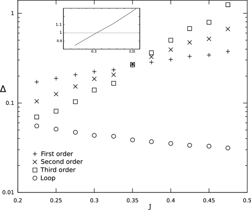
Figure 5.1: Relative error $\Delta$ given in Eq. (5.36) on the inferred couplings as a function of the parameter $J$ of the Sherrington-Kirkpatrick model with $N=200$ spins. Monte Carlo simulations are run over 100 steps. Averages and error bars are computed over 100 samples. Top: orders $\beta$, $\beta^{2}$ and $\beta^{3}$ of the expansion. Bottom: expression (5.35) which includes the sum over all loop diagrams. Inset: largest eigenvalue $\Lambda$ of matrix $M$ as a function of $J$.

If we try to use the same procedure to test the performance of our loop summation formula, we get results like the ones shown in Figure 5.2:

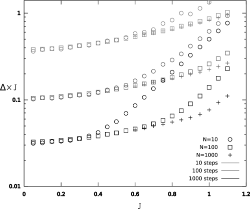
Figure 5.2: Absolute error $J\times\Delta$ on the inferred couplings as a function of the parameter $J$ of the Sherrington-Kirkpatrick model. Inference is done through formula (5.35), which takes into account all loop diagrams. The error decreases with the number of spins and the number of Monte Carlo steps (shown on the figure).

We can clearly see above that the error on the inferred couplings for the Sherrington-Kirkpatrick model is essentially due to the noise in the MC estimates of the correlations and magnetizations, since it decreases with the number of steps.

5.2 Combining the two-spin expansion and the loop diagrams

In the previous section, we have identified a set of diagrams whose sum yields the mean-field approximation we saw in chapter 2. In section 3.1, we have inferred exactly the value of $J$ for a system composed of only two spins (Eqs. (3.6-3.9)). We will see that it is easy to identify summable diagrams also in this two-spin case. Our system is composed only by two spins $i$ and $j$, thus there can be no diagrams of more than two vertices in the expansion of $S$. Moreover, since the formula is exact, the expansion in the case of two spins contains all the two-spin diagrams. Indeed, the first four terms of the Taylor expansion of Eq. (3.7) on small $c_{ij}$ are

$$J_{ij} = \beta K_{ij}-2m_{i}m_{j}K_{ij}^{2}+\frac{1}{3}K_{ij}^{3}\left[1+3m_{i}^{2}+3m_{j}^{2}+9m_{i}^{2}m_{j}^{2}\right]+\ldots\,,$$ (5.40)

$$= \begin{tabular}[]{c}\includegraphics[scale={.4}]{loop1_p}\end{tabular}-2\begin{tabular}[]{c}\includegraphics[scale={.4}]{2spins_3_p}\end{tabular}+\frac{1}{3}\begin{tabular}[]{c}\includegraphics[scale={.4}]{loop_d1_p}\end{tabular}\,.$$

It is easy to identify this formula as the two-spin diagrams in Eq. (4.39). Using the explicit formula for $S^{\text{2-spin}}$ given in Eq. (3.6) and applying Eqs. (3.7–3.9), we obtain

$$S^{\text{2-spin}}_{ij} = S^{\text{1-spin}}_{i}+S^{\text{1-spin}}_{j}$$ (5.41)

$$+\frac{1}{4}\log\left[1+\frac{c_{ij}}{(1-m_{i})(1-m_{j})}\right][c_{ij}+(1-m_{i})(1-m_{j})]$$

$$+\frac{1}{4}\log\left[1-\frac{c_{ij}}{(1-m_{i})(1+m_{j})}\right][c_{ij}-(1-m_{i})(1+m_{j})]$$

$$+\frac{1}{4}\log\left[1-\frac{c_{ij}}{(1+m_{i})(1-m_{j})}\right][c_{ij}-(1+m_{i})(1-m_{j})]$$

$$+\frac{1}{4}\log\left[1+\frac{c_{ij}}{(1+m_{i})(1+m_{j})}\right][c_{ij}+(1+m_{i})(1+m_{j})]\,,$$

where

$$S^{\text{1-spin}}_{i} = -\left[\frac{1+m_{i}}{2}\ln\frac{1+m_{i}}{2}+\frac{1-m_{i}}{2}\ln\frac{1-m_{i}}{2}\right]\,.$$ (5.42)

We have now an explicit formula for the sum of all two-spin diagrams. To go as further as possible in our expansion, we would like to sum both all the loop and 2-spin diagrams. To combine Eq. (5.41) with Eq. (5.23), we need to remove the diagrams that are counted twice, since the loop expansion contains two-spin diagrams (see for ex. the first diagram in Eq. (5.32)). To evaluate the two-spin diagrams of $S^{\text{loop}}$, we can simply evaluate it for the particular case of $N=2$, where all the diagrams involving three or more spins are zero. Thus,

$$S^{\text{loop and 2-spin}}=\frac{1}{2}\log\left[\det\left(\begin{array}[]{cc}1&K_{ij}\sqrt{L_{i}L_{j}}\\ K_{ij}\sqrt{L_{i}L_{j}}&1\end{array}\right)\right]=\frac{1}{2}\log\left(1-K_{ij}^{2}L_{i}L_{j}\right)\,.$$ (5.43)

Finally, we can write an equation combining both sums:

$$S^{\text{2-spin + loop}} = \sum_{i}S^{\text{1-spin}}_{i}+\sum_{i<j}\left[S_{ij}^{\text{2-spin}}-S^{\text{1-spin}}_{i}-S^{\text{1-spin}}_{j}\right]$$ (5.44)

$$+S^{\text{loop}}-\frac{1}{2}\sum_{i<j}\log(1-K_{ij}^{2}L_{i}L_{j})\,.$$

Note that this formula contains all diagrams shown in Eq. (4.38). The corresponding formula for $J_{ij}^{*}$ is

$$J_{ij}^{*(\text{2-spin+loop})} = J_{ij}^{*\text{loop}}+J_{ij}^{*\text{2-spin}}-\frac{K_{ij}}{1-K_{ij}^{2}L_{i}L_{j}}\,,$$ (5.45)

where, as we have already seen in Eq. (3.7),

$$J_{ij}^{*(\text{2-spin})} = \phantom{+}\frac{1}{4}\ln\left[1+K_{ij}(1+m_{i})(1+m_{j})\right]$$ (5.46)

$$+\frac{1}{4}\ln\left[1+K_{ij}(1-m_{i})(1-m_{j})\right]$$

$$-\frac{1}{4}\ln\left[1-K_{ij}(1-m_{i})(1+m_{j})\right]$$

$$-\frac{1}{4}\ln\left[1-K_{ij}(1+m_{i})(1-m_{j})\right]\,.$$

5.2.1 Three spin diagrams

In the case of a system with a zero local magnetization, we can find a rather simple expression for couplings $J_{ij}$ of a system composed of only three spins $\sigma_{i},\sigma_{j},\sigma_{k}$ :

$$\begin{split}J_{ij;k}^{*\text{3-spin}}=&\frac{1}{4}\log\left[\frac{1+c_{ij}-c_{ik}-c_{jk}}{1-c_{ij}-c_{ik}+c_{jk}}\right]\\ -&\frac{1}{4}\log\left[\frac{1-c_{ij}+c_{ik}-c_{jk}}{1-c_{ij}-c_{ik}+c_{jk}}\right]+\frac{1}{4}\log\left[\frac{1+c_{ij}+c_{ik}+c_{jk}}{1-c_{ij}-c_{ik}+c_{jk}}\right]\,.\end{split}$$ (5.47)

Proceeding in the same way we did with the two-spin diagrams, we can combine this formula with the previous results:

$$\begin{split}J_{ij}^{\text{2-spin+loop+3-spin}}=&J_{ij}^{*\text{2-spin+loop}}+\sum_{k\,(k\neq i,k\neq j)}J_{ij;k}^{*\text{3-spin}}-\sum_{k\,(k\neq i,k\neq j)}\Bigg{\{}J_{ij}^{\text{2 spins}}\\ &\phantom{xyzxx}+\frac{c_{ij}-c_{ik}c_{jk}}{1-c_{ij}^{2}-c_{ik}^{2}-c_{jk}^{2}+2c_{ij}c_{jk}c_{ki}}-\frac{c_{ij}}{1-c_{ij}^{2}}\Bigg{\}}\,.\end{split}$$ (5.48)

5.3 Quality of the inference after summing the loops and 2-3 spin diagrams

In this section, we will look at how our results perform for two different well-known models. First we will look analytically at the one-dimensional Ising model and afterwards we will see numerical results for the Sherrington-Kirkpatrick model. We will test both the inference using just the loop diagrams we saw in Eq. (5.33), the combination of loops and two-spin diagrams we saw in Eq. (5.45) and the combination of loops, 2-spins and 3-spins diagrams we saw in Eq. (5.48).

5.3.1 One-dimensional Ising

For the one-dimensional Ising model, we can evaluate exactly the coupling as a function of the correlations (see Eq. (2.5)):

$$J_{kl}=(\delta_{k+1,l}+\delta_{k-1,l})\tanh^{-1}\left(c_{ij}^{\frac{1}{|i-j|}}\right)\,,$$ (5.49)

where $\delta_{ij}$ is the Kronecker symbol. Note that the obtained value of $J_{kl}$ should not depend on the pair of sites $i,j$ chosen. Using our formula for $J_{ij}^{\text{2-spin}}$ given in Eq. (5.46), we have

$$J_{ij}^{\text{2-spin}}=\tanh^{-1}c_{ij}=\tanh^{-1}\left[\left(\tanh J\right)^{|i-j|}\right]\,,$$ (5.50)

which predicts correctly the values of the couplings between closest neighbors $J_{i,i+1}=J$, but gives an non-zero result for the other couplings. On the other hand, using the loop summation formula from Eq. (5.33), we get

$$J_{ij}^{\text{loop}}=\frac{c}{1-c^{2}}\left(\delta_{i,i+1}+\delta_{i,i-1}\right)\,,$$ (5.51)

where $c=c_{i,i+1}=\tanh J$ and $\delta_{i,j}$ is the Kronecker function. The loop sum correctly predicts that the model has only closest-neighbor couplings but does not predict correctly its value.

Finally, using both the 2-spin diagrams and the loop sum (see Eq. (5.45)), we have

$$J_{ij}^{\text{2-spin+loop}} = J(\delta_{i,i+1}+\delta_{i,i-1})+\left[\tanh c_{ij}-\frac{c_{ij}}{1-c_{ij}^{2}}\right](1-\delta_{i,i+1})(1-\delta_{i,i-1})$$ (5.52)

$$= J(\delta_{i,i+1}+\delta_{i,i-1})+O(c^{6})\ ,$$

which is correct to the order $O(c^{6})$. As we will see in the following, the next contribution to the couplings coming from the expansion in Eq. (5.62) corresponds to , whose leading term is indeed proportional to $c_{i,i+2}\cdot c_{i,i+1}^{2}\cdot c_{i+1,i+2}^{2}=c^{6}$.

5.3.2 Sherrington-Kirkpatrick model

In section 5.1, we saw that when we used Monte-Carlo simulations to evaluate the quality of the inference for the SK model we were limited mostly by the numerical errors of the MC simulation. To have more precise values, we now evaluate the error due to our truncated expansion using a program that calculates $c_{ij}$ through an exact enumeration of all $2^{N}$ spin configurations. We are limited to small values of $N$ (10, 15 and 20). However the case of a small number of spins is particularly interesting since, for the SK model, the summation of loop diagrams is exact in the limit $N\rightarrow\infty$, as we discussed in section 2.3. The importance of terms not included in the loop summation is thus better studied at small $N$.

We compared the quality of the inference using the loop summation (Eq. (5.33)), the combination of loop summation and all diagrams up to three spins (Eq. (5.48)) and the method of susceptibility propagation we discussed in section 3.3.2. Results are shown in Figure 5.3. The error is remarkably small for weak couplings (small $J$), and is dominated by finite-digit accuracy ($10^{-13}$) in this limit. Not surprisingly it behaves better than simple loop summation, and also outperforms the susceptibility propagation algorithm.

Figure 5.3: Relative error $\Delta$ (Eq. (5.36)) as a function of $J$ for the SK model for our summation $J_{ij}^{\text{2 spin + loop + 3 spin}}$ (Eq. (5.48)) compared to the Susceptibility Propagation method of Mézard and Mora [Mezard 08] and loop resummation $J_{ij}^{\text{loop}}$ (Eq. (5.33)).

5.4 Numerical evaluation of high-order diagrams

In the two last sections we saw that summing all loop diagrams improved considerably the robustness of the inference. In this section, we will try to find some more terms numerically, in the hope that we might find other classes of exactly summable diagrams. We will proceed in a similar way as in section 4.4.2, where we used a numerical fit to validate our expansion in small $\beta$. We will use the same method to find new diagrams in the expansion by guessing a general form of the lowest-order missing terms and finding numerically their coefficients.

We started by defining a list of several possible corrections to Eq. (5.44) (since Eq. (5.48) is only valid for $m_{i}=0$) such as

$$\begin{split}S=S^{\text{2-spin + loop}}&\\ +\sum_{i,j,k}K_{ij}K_{jk}^{2}K_{ki}^{2}\large[&a_{1}+a_{2}(m_{i}+m_{j})+a_{3}(m_{j}+m_{i})m_{k}+a_{4}m_{i}m_{j}\\ &+a_{5}(m_{i}^{2}+m_{j}^{2})+a_{6}m_{k}^{2}+a_{7}(m_{i}^{3}+m_{j}^{3})\\ &+a_{8}m_{k}^{3}+a_{9}m_{i}m_{j}m_{k}+a_{10}m_{i}m_{j}m_{k}^{2}\large]\,.\end{split}$$ (5.53)

Note that in the same way as in Eq. (4.38), the numerical coefficients in the expansion must be a fraction of small integers, as a consequence of our expansion procedure.

We followed the same method described in section 4.4.2 for each one of our guesses. We found that for all of them, with the exception of the one shown in Eq. (5.53), the fitted coefficients did not correspond to a fraction of small integers as required. Unlikewise, for the guess shown in Eq. (5.53) all the coefficients were zero except $a_{4}=-1$ and $a_{10}=1$. If eventually there was one extra term missing in Eq. (5.53) (for example a term on $K_{ij}^{3}K_{jk}K_{ki}$), the parameters other than $a_{4}$ and $a_{10}$ would have some bogus value to compensate for the missing term. Accordingly, finding only two non-zero coefficients is a strong evidence of the lack of additional corrections other than those shown in Eq. (5.53). Indeed, this is corroborated by the value of the squared mean deviation, which is of the same order as $c^{6}$, as we would expect in an expansion with no supplementary term on $c^{5}$ missing. Finally, the expansion up to order $O(c^{5})$ is given by

$$S=S^{\text{2-spin + loop}}-\sum_{i,j,k}K_{ij}K_{jk}^{2}K_{ki}^{2}m_{i}m_{j}L_{i}L_{j}L_{k}^{2}+O(c^{6})\,.$$ (5.54)

In the particular case of a system with zero magnetization, the guesses of the corrections are much simpler since there is no arbitrary polynomial on $m$ multiplying each term. We could then find all the terms of the expansion up to $O(c^{8})$:

$$S = S^{\text{2-spin+loop}}-\frac{1}{6}\begin{tabular}[]{c}\includegraphics[scale={.4}]{loop_d2}\end{tabular}+\frac{2}{3}\begin{tabular}[]{c}\includegraphics[scale={.4}]{o7}\end{tabular}-\frac{1}{4}\begin{tabular}[]{c}\includegraphics[scale={.4}]{3spins_lin2}\end{tabular}$$ (5.62)

$$-2\begin{tabular}[]{c}\includegraphics[scale={.4}]{o8_3}\end{tabular}+\frac{1}{8}\begin{tabular}[]{c}\includegraphics[scale={.4}]{loop_d3}\end{tabular}+\frac{1}{2}\begin{tabular}[]{c}\includegraphics[scale={.4}]{o8_2}\end{tabular}+O(c^{9})\,.$$

5.5 Expansion in n-spin diagrams

All the results seen up to now were only valid on a small correlation limit. Unfortunately, for actual neuron data, there might be two or more neurons with very strongly correlated activity. Consequently, here we will try another approach, based on the fact that neurons spend the most of their time at rest. Their magnetization is thus very close to $-1$ (or $+1$, depending on which convention one chooses for the rest state). We derive thus an expansion of the couplings valid for values of magnetization close to $\pm 1$. The technical details can be found on appendix B. Our final result is

$$J_{ij}^{\text{k-spin diagrams}} = J_{ij}^{\text{2-spin}}+J_{ij}^{\text{3-spin}}+\ldots J_{ij}^{\text{$k$-spin}}-\text{(repeated diagrams)}\,,$$ (5.63)

and the error is given by

$$J_{ij}^{*} = J_{ij}^{\text{k-spin diagrams}}+O\left[(1-m_{i}^{2})^{k-2}\right]\,.$$ (5.64)

where $J_{ij}^{\text{k-spin}}$ is the sum of all diagrams in the expansion of $J_{ij}$ involving $k$ spins.

The results seen previously in this work (see Eq. (4.38)) suggest that $J_{ij}^{\text{k-spins}}$ is of order $O(c^{k})$, with the lowest order diagram being the loop over $k$ spins, thus

$$J_{ij}^{*}=J_{ij}^{\text{k-spin diagrams}}+O\left(c^{k+1}\right)\,.$$ (5.65)

We can then expect that summing all diagrams up to $k$ spins might be a very good approximation both in the strong magnetization regime (see Eq. (5.64)) and in the week correlation one (see Eq. (5.65)).

Unfortunately, even for values of $k$ as small as $k=4$, we cannot find an exact expression for $J_{ij}^{\text{k-spin}}$ as we did for $k=2$ in Eq. (3.7). In their PNAS paper, Cocco et al. [Cocco 09] note that $J_{ij}^{\text{k-spin}}$ can be obtained numerically, by exact enumeration of all $2^{k}$ possible states of a $k$-spin system. Using this method, they could sum all diagrams up to 7 spins. They could also combine this method with summing all loop diagrams, which has improved the performance of their inference.

Part III Inference of Hopfield patterns

In part II, we have seen a very general treatment of the inverse Ising problem. In this part, we are interested in a particular case of the same problem: inferring the patterns of a Hopfield model, introduced in section 2.4.

In chap. 6, we deal with the problem of inferring a set of $p$ patterns from the measured data under the supposition that the number of patterns is a non-extensive quantity. We derive explicit formulas for the patterns as a function of the magnetizations and correlations in both the paramagnetic and ferromagnetic phases of the model in the limit of large system size. Interestingly, for the paramagnetic case we find in the leading order the same formula found in section 5.1 for the loop summation.

The goal of chapter 7 is to find an estimation of how many times one needs to measure a Hopfield system to be able to have a good estimate of its patterns. To this end, we use the concept of Shannon entropy introduced in chapter 3 to estimate the quantity of information we lack about the system. We evaluate explicitly the entropy for a typical realization of the system as a function of the number of measurements. We find that when the system is magnetized according to one of the patterns, we can find this pattern using just a non-extensive number of measures. On the other hand, to find the patterns that were not visited in any of our measures one needs an extensive number of measures.

Chapter 6 Pattern inference for the Hopfield model

Up to this point we have dealt with the problem of inferring a coupling matrix $\{J_{ij}\}$ of a generalized Ising model. In this chapter, we will look at the particular case of a Hopfield model. There are several potential advantages of this model: first, as we saw in section 1.1.2, in some experiments one needs to infer a set of patterns from the measured data. Secondly, we might expect that reducing the number of degrees of freedom might make the inference procedure more stable. Finally, the Hopfield model can be solved analytically and thus we expect to have a better control of the inference errors.

In principle, one could proceed by first inferring the matrix $\{J_{ij}\}$ from the data, as we have done in part II, and then diagonalizing it to extract a set of patterns. The problem with this approach is that it is not optimal from the Bayes point of view: the inferred patterns are not the ones that maximize the a posteriori probability. This is particularly relevant when the assumption that the underlying system is governed by a Hopfield model is just an approximation, as will almost always be the case in biological data. In this case, we cannot guarantee that the patterns obtained by diagonalizing the $\{J_{ij}\}$ matrix are the ones that best describe the data.

This method was carried out in a paper recently published by Haiping Huang  [Huang 10], where several different methods for solving the inverse Ising model was used to find the couplings of a Hopfield model. In their paper, they show that the method presented in chapters 4 and 5 does not perform significantly better than the naive mean-field method for a Hopfield model, which gives yet another reason to look for a method specific to this model.

In this chapter, we suppose that we have measured $L$ configurations of a system that is governed by a Hopfield model. We would like to deduce both the sign and the magnitude of the patterns from the data using a Bayesian inference, as defined in chapter 3. We suppose that we wait long enough between two successive measures so that they show no temporal correlation, i.e., that our configurations constitute an independent and identically distributed sampling of a Boltzmann distribution.

We will first start with the simple, albeit not very useful, case of Hopfield model with a single pattern. In this case, the calculations can be done in a few lines and allow one to get an idea of the structure of the solution for the general case. Afterwards, we deal with the case of any number of patterns $p$, which is the main result of this chapter.

6.1 A simpler case: inference of a single pattern

In this section we suppose that we have measured $L$ independent configurations of system $\sigma^{1},\ldots,\sigma^{L}$, where each configuration are given by $\sigma^{l}=\{\sigma^{l}_{1},\ldots,\sigma_{N}^{l}\}$ and $\sigma_{i}^{l}=\pm 1$. From this data, we can, for example, evaluate the measured correlations and magnetizations

$$m_{i}=\frac{1}{L}\sum_{l=1}^{L}\sigma_{i}^{l}\,,\quad\quad C_{ij}=\frac{1}{L}\sum_{l=1}^{L}\sigma_{i}^{l}\sigma_{j}^{l}\,.$$ (6.1)

We suppose that our system can be described by a Hopfield pattern with a single pattern. Its Hamiltonian is thus given by

$$H(\{\sigma_{i}\})=-\frac{1}{N}\sum_{i<j}\xi_{i}\xi_{j}\sigma_{i}\sigma_{j}\,,$$ (6.2)

where $\xi_{i}$ are real values that describe the pattern, $\sigma_{i}$ are the spin variables and $N$ is the number of spins of the system. The partition function is given by

$$Z(\beta,\{\xi_{i}\}) = \sum_{\{\sigma\}}\exp\left[\frac{\beta}{N}\sum_{i<j}\xi_{i}\xi_{j}\sigma_{i}\sigma_{j}\right]\,.$$ (6.3)

For the rest of this chapter we will avoid the explicit dependence on $\beta$ by performing the change of variables $\xi_{i}\rightarrow\xi_{i}/\sqrt{\beta}$. We will also omit the dependence of the partition function on $\{\xi_{i}\}$ to simplify notations, posing $Z(\beta,\{\xi_{i}\})\equiv Z$.

We would like to infer both the sign and magnitude of $\xi_{i}$ from the measured configurations $\{\sigma^{l}\}$. Using the Bayes theorem as announced in Eq. (3.10), the likelihood of the patterns is given by

$$P(\{\xi_{i}\}|\{\sigma^{l}\})=\frac{P_{0}(\{\xi_{i}\})}{Z^{L}P(\{\sigma^{l}\})}\prod_{l=1}^{L}\exp\left[\frac{1}{N}\sum_{i<j}\xi_{i}\xi_{j}\sigma_{i}^{l}\sigma_{j}^{l}\right]\,.$$ (6.4)

Using Eq. (6.1), we can rewrite this expression as

$$\begin{split}\frac{1}{L}\log P(\{\xi_{i}\}|\{\sigma^{l}\})=&-\log Z-\log P(\{\sigma^{l}\})\\ &+\frac{1}{L}\log P_{0}(\{\xi_{i}\})+\exp\left[\frac{1}{N}\sum_{i<j}C_{ij}\xi_{i}\xi_{j}\right]\,.\end{split}$$ (6.5)

To maximize this expression, we need to evaluate $\log Z$ explicitly. Using an integral transform, Eq. (6.3) becomes

$$Z = \int_{-\infty}^{\infty}\frac{\mathrm{\;d}x}{\sqrt{2\pi N^{-1}}}\sum_{\{\sigma\}}\exp\left[-\frac{N}{2}x^{2}+x\sum_{i}\xi_{i}\sigma_{i}\right]\,,$$ (6.6)

$$= \int_{-\infty}^{\infty}\frac{\mathrm{\;d}x}{\sqrt{2\pi N^{-1}}}\exp\left\{-\frac{N}{2}x^{2}+\sum_{i}\log\left[2\cosh(x\xi_{i})\right]\right\}\,.$$ (6.7)

In the following, we will set the prior to $P_{0}(\{\xi_{i}\})=1$, since we can see from Eq. (6.5) that it is irrelevant for large values of $L$. In the following we will treat separately the ferromagnetic case ($m\neq 0$) and the paramagnetic case ($m=0$).

6.1.1 Ferromagnetic case

In the ferromagnetic phase, we can use the saddle-point method to evaluate the integral in Eq. (6.7), yielding

$$\log Z=-\frac{N}{2}x^{2}+\sum_{i}\log\left[2\cosh(x\xi_{i})\right]+O(1/N)$$ (6.8)

with $x$ given by

$$x=\frac{1}{N}\sum_{i}\xi_{i}\tanh(x\xi_{i})\,.$$ (6.9)

To infer $\{\xi_{i}\}$ from the data, we follow the maximum likelihood principle and maximize Eq. (6.5) with respect to $\{\xi_{i}\}$, obtaining

$$\frac{1}{N}\sum_{j}C_{ij}\xi_{j}=x\tanh(m\xi_{i})\,.$$ (6.10)

It is easy to see that for such a system the correlation is dominated by its non-connected part: $C_{ij}=m_{i}m_{j}+O(1/N)$. Applying this result to Eq. (6.10), we obtain

$$\xi_{i} = \frac{1}{x}\tanh^{-1}m_{i}\,,$$ (6.11)

and

$$x^{2} = \frac{1}{N}\sum_{i}m_{i}\tanh^{-1}m_{i}\,.$$ (6.12)

We found that the pattern is simply a function of the local magnetization, what is not very surprisingly knowing we are dealing with the ferromagnetic phase.

6.1.2 Paramagnetic case

In the paramagnetic case, the saddle point is $x=0$. Consequently, we need to evaluate the next term in the large $N$ limit to find a non-trivial partition function:

$$Z = \int_{-\infty}^{\infty}\frac{\mathrm{\;d}m}{\sqrt{2\pi N^{-1}}}\exp\left\{-\frac{N}{2}m^{2}+\sum_{i}\log\left[2\cosh(m\xi_{i})\right]\right\}\,,$$ (6.13)

$$= \int_{-\infty}^{\infty}\frac{\mathrm{\;d}m}{\sqrt{2\pi N^{-1}}}\exp\left\{-\frac{N}{2}m^{2}+\frac{m^{2}}{2}\sum_{i}\xi_{i}^{2}\right\}\,,$$

$$= \left(1-\frac{1}{N}\sum_{i}\xi_{i}^{2}\right)^{-\frac{1}{2}}\,.$$

Maximizing with respect to $\xi_{i}$, we obtain

$$\sum_{j}C_{ij}\xi_{j}=\frac{1}{1-\frac{1}{N}\sum_{j}\xi_{j}^{2}}\xi_{i}\,.$$ (6.14)

We conclude thus that $\xi_{i}$ is proportional to an eigenvector $v_{i}$ of the matrix $C$. The corresponding eigenvalue $\lambda$ allows one to find the proportionality constant

$$\xi_{i}=\sqrt{1-\frac{1}{\lambda}}\,v_{i}\,,$$ (6.15)

where the eigenvectors are normalized in the following way

$$\frac{1}{N}\sum_{j}v_{i}^{2}=1\,.$$ (6.16)

It still remain to be decided which pair of eigenvalue/eigenvector we should pick to obtain our pattern. Since we suppose our patterns are real-valued, Eq. (6.15) implies that we should choose an eigenvector greater than one. Moreover, if more than one eigenvalue satisfy this condition, we can easily deduce from Eqs. (6.15), (6.16) and (6.4) that the greatest eigenvalue is the one that maximizes the likelihood.

We verified this formula using Monte-Carlo simulations and the inferred patterns showed a good agreement with the real ones used to make the simulation.

6.2 Inference of continuous patterns for p ¿ 1

In this section, we look at the more general and interesting case of a system with several patterns. In the same way as in the previous section, we will treat the ferro- and paramagnetic case separately. But first, however, we show how the problem is theoretically harder to define in this case.

6.2.1 Discussion on the gauge

A major issue in the inference of the patterns of the Hopfield model is that if the patterns can take real values the problem is ill-defined: there are many patterns that could describe equally well the data. Suppose for example the case $p=2$:

$$H=N\left(\frac{1}{N}\sum_{i}\xi_{i}^{1}\sigma_{i}\right)^{2}+N\left(\frac{1}{N}\sum_{i}\xi_{i}^{2}\sigma_{i}\right)^{2}\,.$$ (6.17)

If we define alternative patterns $\tilde{\xi_{i}^{1}}=\xi_{i}^{1}\cos\theta+\xi_{i}^{2}\sin\theta$ and $\tilde{\xi_{i}^{2}}=-\xi_{i}^{1}\sin\theta+\xi_{i}^{2}\cos\theta$, our new Hamiltonian is

$$\tilde{H} = N\left[\frac{1}{N}\sum_{i}(\xi_{i}^{1}\cos\theta+\xi_{i}^{2}\sin\theta)\sigma_{i}\right]^{2}$$ (6.18)

$$+N\left[\frac{1}{N}\sum_{i}(-\xi_{i}^{1}\sin\theta+\xi_{i}^{2}\cos\theta)\sigma_{i}\right]^{2}\,,$$

$$= H\,.$$ (6.19)

More generally, if one has $p$ patterns, doing a rotation in $p$ dimensions will not change the Hamiltonian of the system. We say that the model has a gauge invariance in respect to such rotations. Thus, for inferring the patterns one need either to add additional constraints to the remove the $p(p-1)/2$ degrees of freedom or to add a prior probability to the patterns, which would select a particular preferred rotation. In the following, we will choose the former solution, since it makes our calculations simpler.

6.2.2 Ferromagnetic phase

Suppose that we have a sample of $L$ measures of our system, containing $l_{1}$ measures where the system was magnetized according to the first patterns, $l_{2}$ measures with the system magnetized according to the second and so on. In this case, we have

$$C_{ij} = \frac{1}{L}\sum_{l}\sigma_{i}^{l}\sigma_{j}^{l}$$ (6.20)

$$= \sum_{k=1}^{p}\frac{1}{L}\sum_{l\in l_{k}}\sigma_{i}^{l}\sigma_{j}^{l}$$

$$= \frac{1}{L}\sum_{k=1}^{p}l_{k}m_{i}^{k}m_{j}^{k}+O(1/N)\,,$$

where

$$m^{k} = \frac{1}{N}\sum_{i}\xi_{i}^{k}\tanh(m_{k}\xi_{i}^{k})\,,$$ (6.21)

and

$$m^{k}_{i} = \tanh(m^{k}\xi_{i}^{k})\,.$$ (6.22)

A consequence of Eq. (6.20) is that the matrix $C_{ij}$ has exactly $p$ eigenvalues that are extensive and their corresponding eigenvectors are proportional to $m_{i}^{k}$. We can thus easily solve Eqs. (6.20-6.22) by diagonalizing the matrix $C_{ij}$. Note that we did not have fixed a gauge when writing these equations, but considering that $m_{i}^{k}$ are proportional to the eigenvectors of the matrix $C_{ij}$ implies that they are orthogonal. Thus, this procedure is equivalent of choosing the gauge that satisfies:

$$\sum_{i}\tanh(m^{k}\xi_{i}^{k})\tanh(m^{k^{\prime}}\xi_{i}^{k^{\prime}})=0,\quad\text{for $k\neq k^{\prime}$}\,.$$ (6.23)

6.2.3 High external field case

In this section, we will suppose that our external field is strong enough so that the spins are not magnetized according to any of the patterns but only according to the external field. We will be interested in inferrin both the patterns of our model but also the value of the external fields, which might be site-dependent. The calculations that will follow can be considerably simplified by replacing our usual Hamiltonian (Eq. (2.32)) by a slightly different one:

$$H=-\frac{1}{N}\sum_{\mu=1}^{p}\sum_{i<j}\xi_{i}^{\mu}\xi_{j}^{\mu}(\sigma_{i}-\tanh h_{i})(\sigma_{j}-\tanh h_{j})-\sum_{i}h_{i}\sigma_{i}\,.$$ (6.24)

This Hamiltonian can be related to the usual one by a translation on the local fields:

$$h_{i}\rightarrow h_{i}-\sum_{\mu}\sum_{j\,(\neq i)}\xi_{i}^{\mu}\xi_{j}^{\mu}\tanh h_{j}\,.$$ (6.25)

From Eq. (3.10), the a posteriori probability for the inference is then given by

$$\begin{split}P(\{\xi_{i}^{\mu}\}&|\{\sigma^{l}\})=\frac{P_{0}(\{\xi_{i}^{\mu}\})}{Z(\{\xi_{i}^{\mu}\})^{L}P(\{\sigma^{l}\})}\times\\ &\times\prod_{l=1}^{L}\exp\left[\frac{\beta}{N}\sum_{\mu=1}^{p}\sum_{i<j}\xi_{i}^{\mu}\xi_{j}^{\mu}(\sigma_{i}^{l}-\tanh h_{i})(\sigma_{j}^{l}-\tanh h_{j})+\beta\sum_{i}h_{i}\sigma_{i}^{l}\right]\,.\end{split}$$ (6.26)

Introducing the measured values of the magnetizations and of the connected correlation

$$m_{i}=\frac{1}{L}\sum_{l}\sigma_{i}^{l}\,,\quad\quad c_{ij}=\frac{1}{L}\sum_{l}\sigma_{i}^{l}\sigma_{j}^{l}-m_{i}m_{j}\,,$$ (6.27)

we can rewrite our probability as

$$\begin{split}P(\{\xi_{i}^{\mu}\}|&\{\sigma^{l}\})=\frac{P_{0}(\{\xi_{i}^{\mu}\})}{Z(\{\xi_{i}^{\mu}\})^{L}P(\{\sigma^{l}\})}\exp\Bigg{[}\frac{\beta L}{N}\sum_{\mu=1}^{p}\sum_{i<j}\xi_{i}^{\mu}\xi_{j}^{\mu}c_{ij}\\ &+\frac{\beta L}{N}\sum_{\mu}\sum_{i<j}\xi_{i}^{\mu}\xi_{j}^{\mu}(m_{i}-\tanh h_{i})(m_{j}-\tanh h_{j})+\beta L\sum_{i}h_{i}m_{i}\Bigg{]}\,.\end{split}$$ (6.28)

To follow our Bayesian approach of maximizing this probability in respect to the patterns and external fields, we need first to evaluate $\log Z$ explicitly. Since this calculation is straightforward its details can be found in appendix D. We obtain

$$\log Z=\sum_{i}\log(2\cosh h_{i})-\frac{1}{2}\sum_{\mu}\log\chi_{\mu}+\frac{1}{4N}\sum_{\mu,\nu}\frac{s_{\mu\nu}^{2}-r_{\mu\nu}}{\chi_{\mu}\chi_{\nu}}+O(1/N^{3/2})\,,$$

where

$$r_{\mu\nu} = \frac{1}{N}\sum_{i}(\xi_{i}^{\mu})^{2}(\xi_{i}^{\nu})^{2}(1-3\tanh^{2}h_{i})(1-\tanh^{2}h_{i})\,,$$ (6.30)

$$\chi_{\mu} = 1-\frac{1}{N}\sum_{i}(\xi_{i}^{\mu})^{2}(1-\tanh^{2}h_{i})\,,$$ (6.31)

$$s_{\mu\nu} = \frac{1}{\sqrt{N}}\sum_{i}\xi_{i}^{\mu}\xi_{i}^{\nu}(1-\tanh^{2}h_{i})\,.$$ (6.32)

Optimization of the probability

In the following, we will ignore the prior, which is justified in the limit $L\rightarrow\infty$. To maximize Eq. (6.28) one could just maximize the following quantity

$$\log P = \frac{1}{2N}\sum_{i,j,\mu}\xi_{i}^{\mu}\xi_{j}^{\mu}c_{ij}+\frac{1}{2N}\sum_{i,j,\mu}\xi_{i}^{\mu}\xi_{j}^{\mu}(m_{i}-\tanh h_{i})(m_{j}-\tanh h_{j})$$ (6.33)

$$+\sum_{i}h_{i}m_{i}-\log Z\,.$$

As discussed in section 6.2.1, we need to choose a gauge to make our problem well-defined. From Eq. (6.2.3), a natural choice to simplify our equations is adding a Lagrange multiplier $x_{\mu\nu}$ to fix the gauge $s_{\mu\nu}=0$. We obtain thus

$$\begin{split}\log P=\frac{1}{2N}\sum_{i,j,\mu}\xi_{i}^{\mu}\xi_{j}^{\mu}c_{ij}+\frac{1}{2N}\sum_{i,j,\mu}\xi_{i}^{\mu}\xi_{j}^{\mu}(m_{i}-\tanh h_{i})(m_{j}-\tanh h_{j})+\sum_{i}h_{i}m_{i}\\ -\sum_{i}\log(2\cosh h_{i})+\frac{1}{2}\sum_{\mu}\log\chi_{\mu}-\frac{1}{4N}\sum_{\mu,\nu}\frac{r_{\mu\nu}}{\chi_{\mu}\chi_{\nu}}-\frac{1}{N\sqrt{N}}\sum_{\mu\neq\nu}x_{\mu\nu}s_{\mu\nu}\,.\end{split}$$ (6.34)

Optimizing with respect to $h_{i}$, we obtain

$$\begin{split}\frac{\partial\log P}{\partial h_{i}}=0=&m_{i}-\tanh h_{i}-\sum_{\mu}(1-\tanh^{2}h_{i})\xi_{i}^{\mu}\frac{1}{N}\sum_{j}\xi_{j}^{\mu}(m_{j}-\tanh h_{j})\\ &+\sum_{\mu}\frac{(\xi_{i}^{\mu})^{2}}{N\chi_{\mu}}\tanh h_{i}(1-\tanh^{2}h_{i})+O(1/N^{3/2})\,.\end{split}$$ (6.35)

Posing

$$\alpha_{\mu}=\sum_{i}\xi_{i}^{\mu}(m_{i}-\tanh h_{i})\,,$$ (6.36)

we can multiply Eq. (6.35) by $\xi_{i}^{\mu}$ and sum over $i$, yielding

$$\chi_{\nu}\alpha_{\nu} = -\frac{1}{\sqrt{N}}\sum_{\mu}\frac{1}{\chi_{\mu}}\frac{1}{\sqrt{N}}\sum_{i}(\xi_{i}^{\mu})^{2}\xi_{i}^{\nu}\tanh h_{i}(1-\tanh^{2}h_{i})\,.$$ (6.37)

Eq. (6.37) shows that unless the matrix $s_{\mu\nu}$ happens to have an eigenvalue equal to $\chi_{\mu}$, $\alpha_{\mu}$ it is of order $1/\sqrt{N}$. We can then rewrite Eq. (6.35) as

$$m_{i}-\tanh h_{i} = -\frac{1}{N}\sum_{\mu}\frac{(\xi_{i}^{\mu})^{2}}{\chi_{\mu}}\tanh h_{i}(1-\tanh^{2}h_{i})+O(1/N^{3/2})\,.$$ (6.38)

which shows clearly that $m_{i}=\tanh h_{i}+O(1/N)$.

We will now optimize our probability with respect to $\xi_{i}^{\mu}$:

$$\frac{1}{N}\sum_{j}c_{ij}\xi_{j}^{\mu} = \frac{1}{N}\frac{1}{\chi_{\mu}}\xi_{i}^{\mu}(1-\tanh^{2}h_{i})-\frac{1}{N^{2}}\sum_{\nu}\frac{\xi_{i}^{\mu}(\xi_{i}^{\nu})^{2}}{\chi_{\mu}\chi_{\nu}}(1-3\tanh^{2}h_{i})(1-\tanh^{2}h_{i})$$ (6.39)

$$-\frac{1}{N^{2}}\sum_{\mu}\frac{r_{\mu\nu}}{\chi_{\mu}^{2}\chi_{\nu}}\xi_{i}^{\mu}(1-\tanh^{2}h_{i})-\frac{2}{N^{2}}\sum_{\nu(\neq\mu)}x_{\mu\nu}\xi_{i}^{\nu}(1-\tanh^{2}h_{i})$$

$$+O(1/N^{5/2})\,,$$

Where we used the fact that $\frac{1}{N}\alpha_{\mu}(m_{i}-\tanh h_{i})=O(1/N^{5/2})$ to ignore subleading terms. In the following, we will start by solving this equation in the leading order on $N$.

Solution in the leading order

We want to find the solutions $\xi_{i}^{\mu,0}$ and $h_{i}^{0}$ of Eqs. (6.38) and (6.39) up to the leading order on $N$. Ignoring sub-leading terms, this equations are respectively given by

$$\frac{1}{N}\sum_{j}c_{ij}\xi_{j}^{\mu,0} = \frac{1}{N}\frac{1}{\chi_{\mu}}\xi_{i}^{\mu,0}(1-\tanh^{2}h_{i}^{0})\,,$$ (6.40)

and

$$h_{i}^{0} = \tanh^{-1}m_{i}\,.$$ (6.41)

If we define $v_{i}^{\alpha}$ as the eigenvector associated to the eigenvalue $\lambda_{\alpha}$ of the matrix

$$M_{ij}=\frac{c_{ij}}{\sqrt{1-\tanh^{2}h_{i}^{0}}\sqrt{1-\tanh^{2}h_{j}^{0}}}\,,$$ (6.42)

we have

$$\xi_{i}^{\mu,0}=\sqrt{1-\frac{1}{\lambda_{\mu}}}\frac{v_{i}^{\mu}}{\sqrt{1-\tanh^{2}h_{i}^{0}}}\,.$$ (6.43)

Note that the orthogonality of the eigenvectors assures that our gauge $s_{\mu\nu}=0$ is respected.

The procedure of diagonalizing the correlation matrix to extract underlying information is known in the statistics literature by the name of Principal Component Analysis. We already mentioned in the end of section 1.1.2 how this method is currently used to find patterns in neuronal data. It was also used by Ranganathan et al. [Halabi 09] to find functional groups in proteins. Our approach gives a Bayesian justification for using the PCA for neuron data and allows us to write the probability distribution for the measured system: it is just the Boltzmann distribution for the obtained Hopfield model.

Note that Eq. (6.42) implies

$$J_{ij} = \sum_{\alpha}\frac{\lambda_{\alpha}-1}{\lambda_{\alpha}}\frac{v_{i}^{\alpha}v_{j}^{\alpha}}{\sqrt{(1-m_{i}^{2})(1-m_{j}^{2})}}$$ (6.44)

$$= \frac{1}{\sqrt{(1-m_{i}^{2})(1-m_{j}^{2})}}\left[M^{-1}(M-1)\right]_{ij}\,,$$

which is exactly the same formula found in section 5.1 for the loop summation, but using the convention of $M_{ii}=1$ instead of $M_{ii}=0$. While this is an encouraging sign that our calculations are correct, it does not bring any new result. We will thus now try to go beyond the leading terms in $N$ and look for the first correction to this expression.

Sub-dominant corrections

Applying our first approximation of the patterns $\xi^{\mu,0}$ to Eq. (6.38), we can evaluate the first correction to the field $h_{i}$. Posing $h_{i}=h_{i}^{0}+h_{i}^{1}$, we have

$$h_{i}^{1}=\frac{1}{1-\tanh^{2}h_{i}^{0}}\frac{1}{N}\sum_{\mu}\frac{(\xi_{i}^{\mu,0})^{2}}{\chi_{\mu}^{0}}\tanh h_{i}^{0}(1-\tanh^{2}h_{i}^{0})$$ (6.45)

Since now we have a more precise value of $h_{i}$, we can redo the procedure of solving Eq. (6.40) we used for the leading order using this new value. We will denote the obtained patterns $\xi_{i}^{\mu,1}$. Note that $\xi_{i}^{\mu,1}$ is correct up to the leading order in $N$, in the same way as $\xi_{i}^{\mu,0}$, since it neglects the subdominant terms in Eq. (6.39). Finally, to find an expression for the patterns that is correct up to the first leading order, $\xi_{i}^{\mu,2}=\xi_{i}^{\mu,1}+\delta_{i}^{\mu}$, we do a Taylor expansion of the dominant orders of Eq. (6.39) around $\xi_{i}^{\mu}=\xi_{i}^{\mu,1}$:

$$\phantom{=}\frac{1}{N}\sum_{i}c_{ij}\delta_{i}^{\mu}-\frac{1}{N}\frac{1}{\chi_{\mu}}\delta_{i}^{\mu}(1-\tanh^{2}h_{i})+\frac{2}{N^{2}}\sum_{\nu(\neq\mu)}x_{\mu\nu}\xi_{i}^{\nu,1}(1-\tanh^{2}h_{i})$$

$$\phantom{=}-\frac{2}{N^{2}\chi_{\mu}^{2}}\sum_{j}\xi_{i}^{\mu,1}\xi_{j}^{\mu,1}\delta_{j}^{\mu}(1-\tanh^{2}h_{i})(1-\tanh^{2}h_{j})=$$

$$=-\frac{1}{N^{2}}\sum_{\nu}\frac{\xi_{i}^{\mu,1}(\xi_{i}^{\nu,1})^{2}}{\chi_{\mu}\chi_{\nu}}(1-3\tanh^{2}h_{i})(1-\tanh^{2}h_{i})$$

$$\phantom{=}-\frac{1}{N^{2}}\sum_{\mu}\frac{r_{\mu\nu}}{\chi_{\mu}^{2}\chi_{\nu}}\xi_{i}^{\mu,1}(1-\tanh^{2}h_{i})\,.$$ (6.46)

Similarly, our gauge equations $s_{\mu\nu}=0$ yields

$$\frac{1}{\sqrt{N}}\sum_{i}(\xi_{i}^{\mu,1}\delta_{i}^{\nu}+\xi_{i}^{\nu,1}\delta_{i}^{\mu})(1-\tanh^{2}h_{i}^{1})=0\,.$$ (6.47)

At last, Eqs. (6.46) and (6.47) form a non-homogeneous linear system in the variables $\delta_{i}^{\mu}$ and $x_{\mu\nu}$ ($\mu<\nu$) which can be solved numerically by a simple matrix inversion.

6.2.4 Numerical verification

In this section we will verify numerically the correctness of both the inference up to the dominant order shown in Eqs. (6.42) and (6.43) and its subdominant corrections shown in Eqs. (6.46) and (6.47). We will proceed in the following way: first, we will choose a set of patterns $\{\xi_{i}^{\mu}\}$ and fields $\{h_{i}\}$ . Then, we will use a numerical method (that we will explain in the following) to compute the correlations and local magnetizations of the corresponding Hopfield model. Using these quantities, we will use our inference procedure to find the the inferred patterns, both in the dominant order $\{\xi_{i}^{\mu,0}\}$ and with the subdominant corrections $\{\xi_{i}^{\mu,2}\}$. Finally, we will compare the obtained patterns with our initially chosen ones to estimate the quality of our inference.

Numerical evaluation of the correlations of the Hopfield model

To verify the validity of our inference, we needed a numerical method that produced very precise values for the correlations, so we could be sure that any disagreement between the real patterns and the inferred ones were due to shortcomings of the inference procedure and not due to numerical errors. Moreover, we wanted a numerical simulation that scales well for increasing $N$, since our equations are correct in the large $N$ limit.

To be able to satisfy these requirements, we restricted our input patterns and fields to a four-block configuration:

$$\begin{array}[]{cccccccccccccc}&&\lx@intercol\hfil N/4\hfil\lx@intercol&\lx@intercol\hfil N/4\hfil\lx@intercol&\lx@intercol\hfil N/4\hfil\lx@intercol&\lx@intercol\hfil N/4\hfil\lx@intercol\\ \vspace{-.4cm}\hfil&&\lx@intercol\hfil\overbrace{\phantom{\begin{array}[]{ccc}a_{1}&\cdots&a_{1}\end{array}}}\hfil\lx@intercol&\lx@intercol\hfil\overbrace{\phantom{\begin{array}[]{ccc}a_{1}&\cdots&a_{1}\end{array}}}\hfil\lx@intercol&\lx@intercol\hfil\overbrace{\phantom{\begin{array}[]{ccc}a_{1}&\cdots&a_{1}\end{array}}}\hfil\lx@intercol&\lx@intercol\hfil\overbrace{\phantom{\begin{array}[]{ccc}a_{1}&\cdots&a_{1}\end{array}}}\hfil\lx@intercol\\ \xi^{1}&=&\{a_{1},&\cdots,&a_{1},&b_{1},&\cdots,&b_{1},&c_{1},&\cdots,&c_{1},&d_{1},&\cdots,&d_{1}\}\,,\\ \xi^{2}&=&\{a_{2},&\cdots,&a_{2},&b_{2},&\cdots,&b_{2},&c_{2},&\cdots,&c_{2},&d_{2},&\cdots,&d_{2}\}\,,\\ \xi^{3}&=&\{a_{3},&\cdots,&a_{3},&b_{3},&\cdots,&b_{3},&c_{3},&\cdots,&c_{3},&d_{3},&\cdots,&d_{3}\}\,,\\ h&=&\{h_{1},&\cdots,&h_{1},&h_{2},&\cdots,&h_{2},&h_{3},&\cdots,&h_{3},&h_{4},&\cdots,&h_{4}\}\,,\\ \end{array}$$ (6.58)

where $\{a_{i}\},\{b_{i}\}$, etc are real values. Since in our calculations we suppose that $\sum_{i}\xi^{\mu}_{i}\xi^{\nu}_{i}=O(\sqrt{N})$ and $\sum_{i}\xi_{i}^{\mu}\tanh h_{i}=O(\sqrt{N})$, we have restricted our number of patterns to three since it is impossible using four blocks to satisfy these conditions for more patterns. In our simulation we have chosen values of $\{a_{i}\}$, $\{b_{i}\}$, $\ldots\,$ so that the patterns obey our orthogonality condition and that the magnitude of the patterns are small enough not to be too close to the phase transition at $|\xi_{i}^{\mu}|=1$.

With the choice of patterns shown in Eq. (6.58), the partition function is

$$\begin{split}Z=\sum_{\{\sigma\}}\exp\Bigg{\{}&N\sum_{\mu=1}^{3}\Bigg{[}a_{\mu}^{2}\left(\frac{1}{N}\sum_{i=1}^{N/4}\sigma_{i}\right)^{2}+b_{\mu}^{2}\left(\frac{1}{N}\sum_{i=N/4+1}^{N/2}\sigma_{i}\right)^{2}\\ +&c_{\mu}^{2}\left(\frac{1}{N}\sum_{i=N/2+1}^{3N/4}\sigma_{i}\right)^{2}+d_{\mu}^{2}\left(\frac{1}{N}\sum_{i=3N/4+1}^{N}\sigma_{i}\right)^{2}\Bigg{]}\Bigg{\}}\,,\end{split}$$ (6.59)

We can see that the Hamiltonian depends only on $m_{1}=\sum_{i=1}^{N/4}\sigma_{i}$, $m_{2}=\sum_{i=N/4+1}^{N/2}\sigma_{i}$, etc. Now we replace the sum over all the spin configurations by a sum over all possible values of $m_{1}$, $m_{2}$, $m_{3}$ and $m_{4}$, which allows one to evaluate the partition function, the correlations and the magnetizations with a complexity of $O(N^{4})$.

Comparison of the inferred with the real patterns

We cannot directly compare the inferred patterns with the real ones to evaluate the error of our procedure since they might differ in gauge. Thus, we used in our comparison a value that does not depend on the gauge: $J_{ij}=\sum_{\mu}\xi_{i}^{\mu}\xi_{j}^{\mu}$. The results of the comparison of the real patterns with the inferred ones can be seen in the following graph

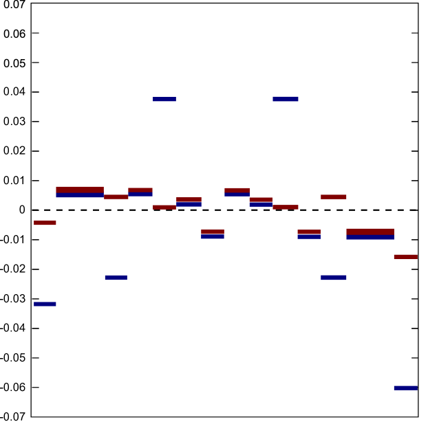
Figure 6.1: Inference error for the different elements of the matrix $J_{ij}$ for $N=100$. In blue we have $J_{ij}^{\text{real}}-\sum_{\mu}\xi_{i}^{\mu,0}\xi_{j}^{\mu,0}$ and in red we have $J_{ij}^{\text{real}}-\sum_{\mu}\xi_{i}^{\mu,2}\xi_{j}^{\mu,2}$. In this graph, we have $\{a_{1},b_{1},c_{1},d_{1}\}=\{0.693,0.4,-0.8,0.4\}$, $\{a_{2},b_{2},c_{2},d_{2}\}=\{0.693,-0.8,0.4,0.4\}$, $\{a_{3},b_{3},c_{3},d_{3}\}=\{0,0.693,0.693,0.693\}$ and $\{h_{1},h_{2},h_{3},h_{4}\}=\{0.254,-0.283,0.416,-0.380\}$.

We can see clearly in Figure 6.1 that the subdominant corrections improve the inference quality. Unfortunately, these corrections are very sensible to noisy data, and we could not see an improvement of the inference for both Monte-Carlo and real neuron data.

Chapter 7 Evaluation of the inference entropy for the Hopfield model

As introduced in section 3.1, a good estimate of how much data is needed to infer a pattern is given by the information-theoretical entropy (Eq. (3.1)) of the a posteriori probability of the patterns, given by

$$S[\{\sigma_{i}^{l}\}]=-\sum_{\{\xi\}}P[\{\xi_{i}^{\mu}\}|\{\sigma_{i}^{l}\}]\log P[\{\xi_{i}^{\mu}\}|\{\sigma_{i}^{l}\}]\,,$$ (7.1)

where $\{\xi_{i}^{\mu}\}$ are the patterns of our Hopfield model (see section 2.4) and $\{\sigma_{i}^{l}\}$ are a set of $L$ measured configurations of the system.

The entropy can be interpreted as the quantity of information that is missing about our system. Thus, when $S\ll 1$, we can say that we have enough data to infer with very little error the patterns. In this chapter we will evaluate the entropy for the inference of the Hopfield model. As before, we will first treat the simpler case of a single pattern before dealing with the more general and interesting case of an arbitrary number of patterns $p$.

7.1 Case of a single binary pattern

Let us recall the usual partition function of the Hopfield model (Eq. (2.32)) for $p=1$

$$Z(\beta,\{\xi_{i}\}) = \sum_{\{\sigma\}}\exp\left[\frac{\beta}{N}\sum_{i<j}\xi_{i}\xi_{j}\sigma_{i}\sigma_{j}\right]\,.$$ (7.2)

In the particular case where $\xi_{i}=\pm 1$, we can pose $\sigma_{i}^{\prime}=\xi_{i}\sigma_{i}$ and rewrite the partition function as

$$Z(\beta)=\sum_{\{\sigma^{\prime}\}}\exp\left[\frac{\beta}{N}\sum_{i<j}\sigma_{i}^{\prime}\sigma_{j}^{\prime}\right]\,.$$ (7.3)

This equation is exactly the same as Eq. (2.6) for zero external field, which means that the thermodynamics of this model is identical to the infinite-dimensional Ising model presented in chapter 2. From a more technical point of view, contrary to the usual Hopfield model with $p>1$, the partition function is independent of the pattern, which make the calculations considerably simpler.

In this case, the Bayes a posteriori probability is given by Eq. (6.4), which we recall here:

$$P(\{\xi_{i}\}|\{\sigma_{i}^{l}\})=\frac{P_{0}(\{\xi_{i}\})}{Z(\beta)^{L}\mathcal{N}(\beta,\{\sigma_{i}^{l}\})}\prod_{l=1}^{L}\exp\left[\frac{1}{N}\sum_{i<j}\xi_{i}\xi_{j}\sigma_{i}^{l}\sigma_{j}^{l}\right]\,,$$ (7.4)

where we used a different notation for the normalization $\mathcal{N}$. Applying this result to Eq. (7.1) and setting the prior $P_{0}(\{\xi_{i}\})=1$, we obtain

$$S[\{\sigma_{i}^{l}\}] = -\frac{1}{\mathcal{N}[\{\sigma_{i}^{l}\}]Z(\beta)^{L}}\sum_{\{\xi\}}\exp\left(\frac{\beta}{N}\sum_{l=0}^{L}\sum_{i<j}\xi_{i}\xi_{j}\sigma_{i}^{l}\sigma_{j}^{l}\right)\times$$ (7.5)

$$\times\left[-\log\left(\mathcal{N}[\{\sigma_{i}^{l}\}]Z(\beta)^{L}\right)+\left(\frac{\beta}{N}\sum_{l=0}^{L}\sum_{i<j}\xi_{i}\xi_{j}\sigma_{i}^{l}\sigma_{j}^{l}\right)\right]\,.$$

Introducing the variable

$$\tilde{N}[\{\sigma_{i}^{l}\}]\equiv\mathcal{N}[\{\sigma_{i}^{l}\}]Z(\beta)^{L}=\sum_{\{\xi\}}\exp\left(\frac{\beta}{N}\sum_{l=0}^{L}\sum_{i<j}\xi_{i}\xi_{j}\sigma_{i}^{l}\sigma_{j}^{l}\right)\,,$$ (7.6)

we can rewrite Eq. (7.5) as

$$S[\{\sigma_{i}^{l}\}] = \frac{\log\tilde{N}[\{\sigma_{i}^{l}\}]}{\tilde{N}[\{\sigma_{i}^{l}\}]}\sum_{\{\xi\}}\exp\left(\frac{\beta}{N}\sum_{l=0}^{L}\sum_{i<j}\xi_{i}\xi_{j}\sigma_{i}^{l}\sigma_{j}^{l}\right)$$ (7.7)

$$-\sum_{\{\xi\}}\frac{\beta}{N}\sum_{l=0}^{L}\sum_{i<j}\xi_{i}\xi_{j}\sigma_{i}^{l}\sigma_{j}^{l}\exp\left(\frac{\beta}{N}\sum_{l=0}^{L}\sum_{i<j}\xi_{i}\xi_{j}\sigma_{i}^{l}\sigma_{j}^{l}\right)$$

$$= \log\tilde{N}[\{\sigma_{i}^{l}\}]-\beta\frac{\partial\log\tilde{N}[\{\sigma_{i}^{l}\}]}{\partial\beta}\,.$$

Thus, the entropy can be trivially evaluated from $\tilde{N}[\{\sigma_{i}^{l}\}]$.

We can see in Eq. (7.6) that the expression for $\tilde{N}$ is formally identical to the partition function of a Hopfield model where the $L$ measured configurations $\{\sigma_{i}^{l}\}$ play the role of the patterns and $\{\xi_{i}\}$ replace the spin variables:

$$Z_{\text{Hop}}=\sum_{\{\sigma\}}\exp\left(\frac{\beta}{N}\sum_{\mu=1}^{L}\sum_{i<j}\xi_{i}^{\mu}\xi_{j}^{\mu}\sigma_{i}\sigma_{j}\right)\,.$$ (7.8)

For such analogy, the inference entropy shown in Eq. (7.7) has a thermodynamic meaning: it is the thermodynamic entropy of the model.

Eqs. (7.6) and (7.7) give the entropy of the system for a particular set of measures $\{\sigma_{i}^{l}\}$. Now, it is natural to expect the entropy to be very reproducible across different sets of measurements. In this context, we are interested in evaluating the average of the entropy with respect to all possible measurements. Supposing that the data is produced measuring an actual Hopfield model with a pattern $\{\tilde{\xi}_{i}\}$, we have

$$\left\langle S\right\rangle = \left.\left\langle\log\tilde{N}[\{\sigma_{i}^{l}\}]\right\rangle\right|_{\tilde{\beta}=\beta}-\beta\left(\frac{\partial}{\partial\beta}\left\langle\log\tilde{N}[\{\sigma_{i}^{l}\}]\right\rangle\right)_{\tilde{\beta}=\beta}\,,$$ (7.9)

with

$$\left\langle\log\tilde{N}\right\rangle = \frac{1}{Z\left(\tilde{\beta}\right)^{L}}\sum_{\{\sigma\}}\exp\left(\frac{\tilde{\beta}}{N}\sum_{l=0}^{L}\sum_{i<j}\tilde{\xi_{i}}\tilde{\xi_{j}}\sigma_{i}^{l}\sigma_{j}^{l}\right)\log\tilde{N}[\{\sigma_{i}^{l}\}]\,,$$ (7.10)

where we replaced our usual inverse temperature $\beta$ by a new variable $\tilde{\beta}$ since we should not take the derivative in respect to it in Eq. (7.9).

The entropy of the system is very different if $\beta<1$ and the system is in the paramagnetic phase or if $\beta>1$ in which case the system is in the ferromagnetic phase. We will see these two cases separately in the following sections.

7.1.1 Ferromagnetic case

In the ferromagnetic case, if we want to evaluate a thermal average of some quantity $X$, we have

$$\left\langle X\right\rangle = \frac{1}{Z^{L}(\tilde{\beta})}\sum_{\{\sigma\}}X(\{\sigma_{i}^{l}\})\exp\left(\frac{\tilde{\beta}}{N}\sum_{l=0}^{L}\sum_{i<j}\tilde{\xi_{i}}\tilde{\xi_{j}}\sigma_{i}^{l}\sigma_{j}^{l}\right)\,,$$ (7.11)

$$= \sum_{\{\sigma\}}X(\{\sigma_{i}^{l}\})\prod_{l=1}^{L}\prod_{i=1}^{N}\frac{e^{\tilde{\beta}m^{*}\sigma^{l}_{i}\tilde{\xi}_{i}}}{2\cosh\left(\tilde{\beta}m^{*}\right)}\,,$$

where $m^{*}$ is the solution of the equation $m^{*}=\tanh(\tilde{\beta}m^{*})$.

Since $\log\tilde{N}$ is formally identical to the free-energy of the Hopfield model, we start with the saddle-point solution obtained in chap. 2, given in Eqs. (2.35) and (2.36):

$$\log\tilde{N} = -\frac{\beta N}{2}\sum_{l=1}^{L}m_{l}^{2}+\sum_{i}\log\left[2\cosh\left(\beta\sum_{l=1}^{L}m_{l}\sigma_{i}^{l}\right)\right]\,,$$ (7.12)

and

$$m_{l} = \frac{1}{N}\sum_{i}\sigma_{i}^{l}\tanh\left(\beta\sum_{s}m_{s}\sigma_{i}^{s}\right)\,.$$ (7.13)

We recall that the physical meaning of $m_{\mu}$ in the Hopfield model is the magnetization of the spins according to the pattern $\mu$. In our case, it represents the overlap between the pattern we are inferring and the $l$-th configuration: $m_{l}=\frac{1}{N}\sum_{i}\xi_{i}\sigma_{i}^{l}$.

Eq. (7.13) has always a solution in the form $\{m_{l}\}=\{{m,m,...,m\}}$ [Amit 85a]. Since $\{\sigma_{i}^{l}\}$ are measured configurations of an Ising system in the ferromagnetic phase, we expect them to be very similar: they are all close to the same minimum of the free energy of the Ising model. We expect thus that the solution $\{m_{l}\}=\{{m,m,...,m\}}$ to be the minimum of our modified free-energy of Eq. (7.12). Under this hypothesis, the entropy reads

$$\frac{\left\langle S\right\rangle}{N}=\left\langle\ln\left[2\cosh\left(\beta m\sum_{l}\sigma^{l}\right)\right]\right\rangle-\left\langle\left(\beta m\sum_{l}\sigma^{l}\right)\tanh\left(\beta m\sum_{l}\sigma^{l}\right)\right\rangle\,,$$ (7.14)

where the value of $m$ that satisfies Eq. (7.13) is $m=m^{*}$, fact proven in Appendix E.

Asymptotic behavior

One can note that the entropy of this system is the same of the system composed of a single spin $\rho=\pm 1$ connected with $L$ independent, magnetized spins. The partition function for this system of a single spin is

$$Z=2\cosh\left(\beta m\sum_{i}\sigma_{i}\right)\,,$$ (7.15)

and the free-energy reads

$$F=\left\langle\log\left[2\cosh\left(\beta m\sum_{i}\sigma_{i}\right)\right]\right\rangle_{\sigma_{i}}\,,$$ (7.16)

where the average is done with respect to independent spins $\sigma$ with magnetization $m$. If we want to calculate the average entropy of this system, we note that for large $x$, $\log\left(2\cosh x\right)-x\tanh x\approx(1+2|x|)e^{-2|x|}$. Consequently

$$\left\langle S\right\rangle\approx\sum_{k=0}^{L}\left(\begin{array}[]{c}L\\ k\end{array}\right)\frac{e^{\beta m(L-2k)}}{\left[2\cosh(\beta m)\right]^{L}}e^{-2\beta m|L-2k|}\,.$$ (7.17)

One may remark that the probability that our single spin $\rho$ is not aligned with its partners is exponentially small on $L$. There are two extreme cases that contributes to this probability

1. The spins $\sigma_{i}$ obeys $\sum_{i}\sigma_{i}\approx 0$ (which is very unlikely) and consequently our spin $\rho$ is random.

2. We have the highly probable situation of $\sum_{i}\sigma_{i}\approx mL$, but our spin $\rho$ is misaligned with the others, which is very unlikely.

The case 1 has a probability $\approx\left[\cosh(\beta m)\right]^{-L}$ and gives a $\log 2$ contribution to the entropy, while the case 2 has a probability O(1) but gives a contribution of order $e^{-2\beta m^{2}L}$ to the entropy. Since for all $\beta$, $\log\cosh(\beta m)<2\beta m^{2}$ (note that $m$ is an implicit function of $\beta$) , case 1 dominates the behavior of the system for $L\rightarrow\infty$. So, for large $L$, we have the general behavior

$$S\propto e^{-\gamma L},$$ (7.18)

with

$$\gamma=\log\cosh\left(\beta m\right)\,.$$ (7.19)

We can see how well the entropy converges to this asymptotic behavior in Fig. 7.1.

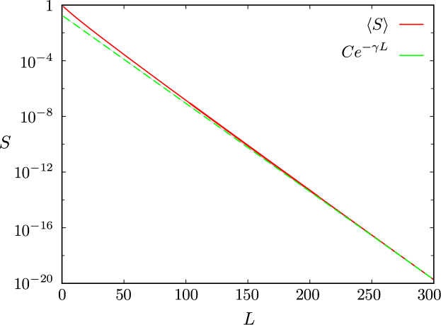
Figure 7.1: Entropy per spin as a function of $L$ for $\beta=1.1$ according to Eq. (7.14).

We can thus conclude that for $L\gg 1/\gamma$ we can infer the unknown pattern with a very small probability of error.

7.1.2 Paramagnetic case

In the paramagnetic phase we have $m=0$. According to Eq. (7.14), the entropy is thus equal to $\log 2$ for all values of $L$. This is correct under the hypothesis that $L$ remains finite when $N\rightarrow\infty$. For $L=\alpha N$, the results of the previous section do not hold since we cannot use the saddle-point approximation for $\log Z$.

We start with Eq. (2.4)

$$\tilde{N}=\int\prod_{l=1}^{L}\frac{\mathrm{\;d}m_{l}}{\sqrt{2\pi\beta^{-1}N^{-1}}}\sum_{\{\xi\}}\exp\left[-\frac{\beta N}{2}\sum_{l=1}^{L}m_{l}^{2}+\beta\sum_{l=1}^{L}m_{l}\sum_{i}\sigma_{i}^{l}\xi_{i}\right]$$ (7.20)

and we would like to find the average $\left\langle\tilde{N}\right\rangle_{\sigma}$ with respect to all possible realizations of the measures $\{\sigma_{i}^{l}\}$, like we have done in the ferromagnetic case. The main difference is that now the saddle-point values of $m_{l}$ are of order $O(1/\sqrt{N})$.

To find the correct solution under these conditions, we need to use the replica trick as explained in section 2.4. The calculations are very similar to those done in the solution of the Hopfield model by Amit et al. [Amit 85b] and the details can be found in Appendix F. The obtained value for the entropy is given by

$$\left\langle S\right\rangle_{\sigma} = -\frac{\alpha\beta(1-q)\left\{1-\beta\left[2-2q(1-\beta)-(1+t^{2})\beta\right]\right\}}{2(1-\beta)\left[1-(1-q)\beta\right]^{2}}-\frac{\alpha}{2}\ln\left[1-(1-q)\beta\right]$$ (7.21)

$$+\left\langle\ln\left[2\cosh\left(\frac{\alpha}{2}\hat{t}+z\sqrt{\alpha\hat{q}}\right)\right]\right\rangle_{z}-\frac{\alpha}{2}\left[(1-q)\hat{q}+t\hat{t}\right]\,,$$

where $\left\langle f\right\rangle_{z}=\int_{-\infty}^{\infty}f(z)e^{-z^{2}/2}\mathrm{\;d}z$, we remind that $\alpha=L/N$ and

$$t = \left\langle\sigma_{i}^{l}\xi_{i}\right\rangle_{\sigma}=\left\langle\tanh\left(\frac{\alpha}{2}\hat{t}+z\sqrt{\alpha\hat{q}}\right)\right\rangle_{z}\,,$$ (7.22)

$$q = \left\langle\left(\frac{1}{N}\sum_{i}\xi_{i}\sigma_{i}^{l}\right)^{2}\right\rangle_{\sigma}=\left\langle\left[\tanh\left(\frac{\alpha}{2}\hat{t}+z\sqrt{\alpha\hat{q}}\right)\right]^{2}\right\rangle_{z}\,,$$ (7.23)

$$\hat{t} = \frac{2t\beta^{2}}{(1-\beta)[1-(1-q)\beta]}\,,$$ (7.24)

$$\hat{q} = \beta^{2}\frac{q(1-\beta)+t^{2}\beta}{(1-\beta)\left[1-(1-q)\beta\right]^{2}}\,,$$ (7.25)

where we remind that $t$ is the overlap between the real and the inferred pattern. One can verify that we only have a non zero solution to these equations when $\alpha>\alpha_{c}$, with $\alpha_{c}=\left(1-\frac{1}{\beta}\right)^{2}$. In this case both $q$ and $t$ are non-zero.

When $\alpha<\alpha_{c}$, $t$ is zero which implies that the inferred pattern has no resemblance to the real one. Surprisingly, the entropy decreases linearly in this regime for increasing $\alpha$, which can be possibly interpreted as a growth of the set of patterns known to be incompatible with the data.

Note that in contradistinction with the ferromagnetic case, to infer the patterns in the paramagnetic phase it takes a number of measures that is proportional to the size of the system, implying that is much harder to extract information from it.

Numerical verification

In Figure 7.2, one can see the behavior of the entropy as a function of $\alpha$ for a fixed inverse temperature $\beta=0.5$.

Figure 7.2: Entropy per spin as a function of $\alpha$ for $\beta=0.5$. The solid line correspond to Eqs. (7.21–7.25) while the points correspond to numerical values obtained by exact enumeration. The dashed line corresponds to the behavior of $\left\langle S\right\rangle$ in the regime of $q=t=0$ while the vertical line indicates $\alpha_{c}$.

To evaluate numerically $\left\langle S\right\rangle$ as shown in Fig. 7.2, we used the following algorithm:

1. Evaluate $Z$ by exact enumeration;

2. Generate $L=\alpha N$ configurations $\{\sigma_{i}^{l}\}$ according to the Boltzmann weight by rejection sampling;

3. Evaluate $\mathcal{N}[\{\sigma_{i}^{l}\}]$ by exact enumeration;

4. Evaluate $S[\{\sigma_{i}^{l}\}]$ by exact enumeration.

For every $\alpha$, we repeated this procedure one hundred times with different random seeds, which gives different configurations $\{\sigma_{i}^{l}\}$ in step 2. The points in the graph correspond to the averages of the set of obtained values of $S$ and the error bars were calculated using the standard deviation. The result of this procedure supports our analytical results. Indeed, in Figure 7.2 we notice that the bigger values of $N$ are much closer to the analytical curve, which suggests that the difference between the analytical and numerical results is due to the small value of $N$ used in the numerical calculations.

7.2 Case of a single pattern $\bm{\xi_{i}\in\mathbb{R}}$

The results of the previous section are valid only if our pattern takes bimodal values, what might be a very particular case. To verify if the inference of a real-valued pattern presents any qualitative difference with respect to the bimodal case, we propose ourselves to evaluate explicitly the entropy for the real-valued case in this section.

The calculations are similar to those of the last section, but with the supplementary complication that the partition function depends on the exact values of the pattern whereas in the bimodal case it depended only on the temperature. The partition function is given by

$$\log Z\left[\{\xi_{i}\}\right] = -\frac{N}{2}m[\{\xi_{i}\}]^{2}+\sum_{i}\log\left[2\cosh(m\xi_{i})\right]\,,$$ (7.26)

with

$$m[\{\xi_{i}\}] = \frac{1}{N}\sum_{i}\xi_{i}\tanh\left(\xi_{i}m[\{\xi\}]\right)\,.$$ (7.27)

Since $\xi_{i}$ is continuous, we must modify the definition of the entropy replacing the sum by an integral

$$S[\{\sigma_{i}^{l}\}] = -\int\prod_{i}\mathrm{\;d}\xi_{i}P[\{\xi_{i}\}|\{\sigma_{i}^{l}\}]\log P[\{\xi_{i}\}|\{\sigma_{i}^{l}\}]\,.$$ (7.28)

Using Bayes’ theorem, we obtain

$$\begin{split}S[\{\sigma_{i}^{l}\}]&=-\frac{1}{\mathcal{N}[\{\sigma_{i}^{l}\}]}\int\prod_{i}\mathrm{\;d}\xi_{i}\,\frac{P_{0}(\{\xi_{i}\})}{Z^{L}(\{\xi_{i}\})}\exp\left(\frac{1}{N}\sum_{l=0}^{L}\sum_{i<j}\xi_{i}\xi_{j}\sigma_{i}^{l}\sigma_{j}^{l}\right)\times\\ &\times\Bigg{[}-\log\mathcal{N}[\{\sigma_{i}^{l}\}]-L\log Z(\{\xi_{i}\})+\log P_{0}(\{\xi_{i}\})\phantom{\frac{A}{B}\sum_{a}^{b}}\\ &\left.\phantom{\Bigg{[}+}+\frac{1}{N}\sum_{l=0}^{L}\sum_{i<j}\xi_{i}\xi_{j}\sigma_{i}^{l}\sigma_{j}^{l}\right]\,,\end{split}$$ (7.29)

where $\mathcal{N}[\{\sigma_{i}^{l}\}]$ is given by

$$\mathcal{N}[\{\sigma_{i}^{l}\}] = \int\prod_{i}\mathrm{\;d}\xi_{i}\,P[\{\xi_{i}\}|\{\sigma_{i}^{l}\}]$$ (7.30)

$$= \int\prod_{i}\mathrm{\;d}\xi_{i}\,\frac{P_{0}(\{\xi_{i}\})}{Z^{L}(\{\xi_{i}\})}\exp\left(\frac{1}{N}\sum_{l=0}^{L}\sum_{i<j}\xi_{i}\xi_{j}\sigma_{i}^{l}\sigma_{j}^{l}\right)\,.$$ (7.31)

As in the previous section, we would like to write $S$ as a derivative of the normalization. For that, we define a modified normalization $\tilde{N}$ by introducing a parameter $\beta$ to $\mathcal{N}$:

$$\begin{split}\tilde{N}[\{\sigma_{i}^{l}\},\beta]&=\\ =\int\prod_{i}&\mathrm{\;d}\xi_{i}\exp\left(\frac{\beta}{N}\sum_{l=0}^{L}\sum_{i<j}\xi_{i}\xi_{j}\sigma_{i}^{l}\sigma_{j}^{l}+\beta\log P_{0}(\{\xi_{i}\})-\beta L\log Z(\{\xi_{i}\})\right)\,.\end{split}$$ (7.32)

Note that while $\beta$ is similar to a inverse temperature, it is not strictly one, since it multiplies also the partition function. Using this definition, we can rewrite our entropy as

$$S[\{\sigma_{i}^{l}\}]=\log\tilde{N}[\{\sigma_{i}^{l}\},1]-\left.\frac{\partial\log\tilde{N}[\{\sigma_{i}^{l}\},\beta]}{\partial\beta}\right|_{\beta=1}\,.$$ (7.33)

A supplementary difficulty of the continuous case is the dependence of $\log Z$ on $m[\{\xi\}]$, which depends on the patterns implicitly according to Eq. (7.27). To make that dependence explicit, we introduce the following identity

$$f(m[\xi])=\int\mathrm{\;d}m\int\mathrm{\;d}xf(m)\exp\left[-iNxm+i\sum_{i}\xi_{i}\tanh(m\xi_{i})\right]\,,$$ (7.34)

which is just Dirac’s delta written in the integral form. We can thus write the $e^{-\beta L\log Z}$ term in Eq. (7.32) as

$$\begin{split}e^{-\beta L\log Z}=\int\mathrm{\;d}m\int\mathrm{\;d}x\exp\Bigg{\{}\frac{\beta LN}{2}m^{2}&-\beta L\sum_{i}\log\left[2\cosh(m\xi_{i})\right]\\ &-iNxm+i\sum_{i}\xi_{i}\tanh(m\xi_{i})\Bigg{\}}\,.\end{split}$$ (7.35)

Like in the previous section, we would like to evaluate the average of the entropy with respect to the different possible measures and to the different real pattern $\{\tilde{\xi}_{i}\}$:

$$\left\langle S\right\rangle=\int\prod_{i}\mathrm{\;d}\tilde{\xi}_{i}\,P_{0}(\{\tilde{\xi}_{i}\})\sum_{\sigma}\frac{1}{Z(\{\tilde{\xi_{i}}\})}S(\{\sigma_{i}^{l}\})\exp\left[\frac{1}{N}\sum_{l=1}^{L}\sum_{i<j}\tilde{\xi}_{i}\tilde{\xi}_{j}\sigma_{i}^{l}\sigma_{j}^{l}\right]$$ (7.36)

where we impose that the distribution of the unknown real patterns $\{\tilde{\xi}_{i}\}$ is the same of our prior distribution $P_{0}(\{\xi_{i}\})$.

The details of the replica calculation, similar to the last section, can be found in Appendix G. It yields

$$\begin{split}\frac{1}{N}&\left\langle\log\tilde{N}\right\rangle=\frac{\beta}{2}\sum_{l=1}^{L}Q_{l}^{2}+\frac{\beta Lm^{2}}{2}\\ &+\int\mathrm{\;d}\tilde{\xi}\,p_{0}(\tilde{\xi})\sum_{\{\sigma^{l}\}}\exp\left[\tilde{m}\tilde{\xi}\sum_{l=1}^{L}\sigma^{l}-L\log(2\cosh(\tilde{m}\tilde{\xi}))\right]\times\\ &\phantom{\int}\times\log\left\{\int\mathrm{\;d}\xi\exp\left[\beta\sum_{l=1}^{L}Q_{l}\xi\sigma^{l}-\beta L\log(2\cosh(m\xi))+\beta\log p_{0}(\xi)\right]\right\}\,,\end{split}$$ (7.37)

where

$$\tilde{m} = \int\mathrm{\;d}\tilde{\xi}\,p_{0}(\tilde{\xi})\,\tilde{\xi}\tanh(\tilde{m}\tilde{\xi})=\left\langle\tilde{\xi}\tanh(\tilde{m}\tilde{\xi})\right\rangle\,,$$ (7.38)

$$m = \int\mathrm{\;d}\tilde{\xi}\,\sum_{\{\sigma\}}\exp\left[\sum_{l=1}^{L}\tilde{m}\tilde{\xi}\sigma^{l}-L\log 2\cosh(\tilde{m}\tilde{\xi})\right]\times$$ (7.39)

$$\times\frac{\int\mathrm{\;d}\xi\,p_{0}(\xi)\xi\tanh(m\xi)\exp\left[\sum_{l=1}^{L}Q^{l}\sigma^{l}\xi-L\log 2\cosh(m\xi)\right]}{\int\mathrm{\;d}\xi\,p_{0}(\xi)\exp\left[\sum_{l=1}^{L}Q^{l}\sigma^{l}\xi-L\log 2\cosh(m\xi)\right]}\,,$$

$$Q_{k} = \int\mathrm{\;d}\tilde{\xi}\,\sum_{\{\sigma\}}\exp\left[\sum_{l=1}^{L}\tilde{m}\tilde{\xi}\sigma^{l}-L\log 2\cosh(\tilde{m}\tilde{\xi})\right]\times$$ (7.40)

$$\times\frac{\int\mathrm{\;d}\xi\,p_{0}(\xi)\xi\sigma^{l}\exp\left[\sum_{l=1}^{L}Q^{l}\sigma^{l}\xi-L\log 2\cosh(m\xi)\right]}{\int\mathrm{\;d}\xi\,p_{0}(\xi)\exp\left[\sum_{l=1}^{L}Q^{l}\sigma^{l}\xi-L\log 2\cosh(m\xi)\right]\,,}$$

and $\prod_{i}e^{p_{0}(\xi_{i})}=P_{0}(\{\xi\})$ is the prior probability of the pattern and the probability distribution we used to average over the real pattern, supposed to be identical.

From this last equation it is straightforward to evaluate the entropy using Eq. (7.33).

7.3 Case of a system with p patterns, magnetized following a strong external field

In this section we consider the same conditions as we had in section 6.2.3 for the inference: we have a Hopfield model with $p$ patterns and we introduce a local external field strong enough so that the system is not magnetized according to any of the patterns. The Hamiltonian is thus the same as Eq. (2.32). The calculations are very similar to these of section 7.4, so they can be found in Appendix I. We find that the entropy associated with each one of the patterns is described by exactly the same equations as single pattern in the paramagnetic phase, seen in section 7.1.2. We have thus the same behavior: we need thus a number of measures that is proportional to the size of the system and the exact form of the entropy is given by Eqs. (7.21–7.25).

7.4 A particular case: a system with two patterns, magnetized according to the first

In last section, we saw that when our system does not visit any one of the patterns the inference of each one of them is as hard as describing a system composed of a single pattern in the paramagnetic phase. In this section, we will see if there is any qualitative change in the situation where the system is magnetized according to one pattern but we would like to infer a second, non-visited one.

We suppose that our system’s Hamiltonian is given by

$$H=-\beta\sum_{i<j}(\xi_{i}^{1}\xi_{j}^{1}+\xi_{i}^{2}\xi_{j}^{2})\sigma_{i}\sigma_{j}\,,$$

where the patterns $\xi_{i}^{\mu}=\pm 1$ are binary. We suppose we did $L=\alpha N$ measures of the configuration of this system, all of them while the system was magnetized following the first pattern. Supposing that the first pattern is perfectly known (what is reasonable since our entropy on it goes with $e^{-\gamma L}=e^{O(N)}$ as the inference of the first pattern is very similar to the ferromagnetic case we saw previously), we study the entropy of the a posteriori distribution of the second pattern

$$S=-\sum_{\{\xi^{2}_{i}\}}P[\{\xi^{2}_{i}\}|\{\xi^{1}_{i}\},\{\sigma^{l}_{i}\}]\log P[\{\xi^{2}_{i}\}|\{\xi^{1}_{i}\},\{\sigma^{l}_{i}\}]\,.$$ (7.41)

In the same way we did with the single pattern case in section 7.1, we average this entropy with respect both to the first pattern and to the measured configurations. The probability is given by

$$P[\{\xi^{2}_{i}\}|\{\xi^{1}_{i}\},\{\sigma^{l}_{i}\}] = \frac{P[\{\sigma^{l}_{i}\}|\{\xi^{1}_{i}\},\{\xi^{2}_{i}\}]P[\{\xi^{2}_{i}\}]}{\mathcal{N}[\{\xi^{1}_{i}\},\{\sigma^{l}_{i}\}]}\,,$$ (7.42)

$$P[\{\sigma^{l}_{i}\}|\{\xi^{1}_{i}\},\{\xi^{2}_{i}\}] = \frac{1}{Z_{\text{Hop}}[\beta,\{\xi^{1}_{i}\},\{\xi^{2}_{i}\}]^{L}}\exp\left[\frac{\beta}{N}\sum_{\mu=1,2}\sum_{l=1}^{L}\sum_{i<j}\sigma_{i}^{l}\sigma_{j}^{l}\xi_{i}^{\mu}\xi_{j}^{\mu}\right]\,,$$

where the normalization of the probability $\mathcal{N}$ is given by

$$\mathcal{N}[\{\xi^{1}\},\{\sigma^{l}\}] = \sum_{\{\xi^{2}\}}\frac{1}{Z_{\text{Hop}}[\beta,\{\xi^{1}\},\{\xi^{2}\}]^{L}}\exp\left[\frac{\beta}{N}\sum_{\mu=1,2}\sum_{l=1}^{L}\sum_{i<j}\sigma_{i}^{l}\sigma_{j}^{l}\xi_{i}^{\mu}\xi_{j}^{\mu}\right]P[\xi^{2}]\,.$$

As done in Section 7.1, we write our entropy as a derivative of a modified normalization $\tilde{N}$ given by

$$\tilde{N}[\{\xi^{1}\},\{\sigma^{l}\}] = \sum_{\{\xi^{2}\}}\exp\Bigg{[}\frac{\beta}{N}\sum_{\mu=1,2}\sum_{l=1}^{L}\sum_{i<j}\sigma_{i}^{l}\sigma_{j}^{l}\xi_{i}^{\mu}\xi_{j}^{\mu}$$ (7.45)

$$-\frac{\beta}{\tilde{\beta}}L\log Z_{\text{Hop}}[\tilde{\beta},\{\xi^{1}\},\{\sigma^{l}\}]\Bigg{]}\,,$$

so that we can easily deduce the entropy as

$$S = \left.\log\tilde{N}\right|_{\beta=\tilde{\beta}}-\left.\frac{\partial\log\tilde{N}}{\partial\beta}\right|_{\beta=\tilde{\beta}}\,,$$ (7.46)

where we have supposed $P[\xi^{2}]=2^{-N}$. We will now evaluate this quantity explicitly.

Doing a calculation very similar to the derivation of Eq. (6.2.3), we can write the partition function of the Hopfield model for $p=2$ for a system magnetized in the first pattern, obtaining:

$$\log Z_{\text{Hop}} = -\frac{\beta N}{2}m^{*2}+N\log\left[2\cosh(\beta m^{*})\right]-\log\left[1-\beta(1-m^{*2})\right]$$ (7.47)

$$+\frac{1}{2}\frac{\beta m^{*2}}{1-\beta(1-m^{*2})}\left[\frac{1}{\sqrt{N}}\sum_{i}\xi^{1}_{i}\xi^{2}_{i}\right]^{2}\,,$$

with $m^{*}$ given by $m^{*}=\tanh(\beta m^{*})$.

7.4.1 Evaluation of $\bm{\langle}$log Ñ$\bm{\rangle}$

To evaluate $\left\langle\log\tilde{N}\right\rangle$, we use again the replica trick, obtaining

$$\begin{split}\left\langle N^{n}\right\rangle=&\frac{1}{2^{N}}\sum_{\{\xi^{1}\}}\frac{1}{2^{N}}\sum_{\{\tilde{\xi}^{2}\}}\sum_{\{\sigma\}}\sum_{\{\xi^{2,\nu}\}}\exp\Bigg{\{}\\ &\frac{\beta}{N}\sum_{\nu=1}^{n}\sum_{l=1}^{L}\sum_{i,j}\sigma_{i}^{l}\sigma_{j}^{l}(\xi_{i}^{1}\xi_{j}^{1}+\xi_{i}^{2,\nu}\xi_{j}^{2,\nu})-\frac{\beta}{\tilde{\beta}}L\sum_{\nu=1}^{n}\log Z_{\text{Hop}}\left[\tilde{\beta},\{\xi^{1}\},\{\xi^{2,\nu}\}\right]\\ &+\tilde{\beta}\sum_{l=1}^{L}\sum_{i,j}\sigma_{i}^{l}\sigma_{j}^{l}(\xi_{i}^{1}\xi_{j}^{1}+\tilde{\xi}^{2}_{i}\tilde{\xi}^{2}_{j})-L\log Z_{\text{Hop}}\left[\tilde{\beta},\{\tilde{\xi}^{1}\},\{\tilde{\xi}^{2}\}\right]\Bigg{\}}\,,\end{split}$$ (7.48)

where we denote by $\tilde{\xi^{2}}$ the real second pattern and by $\xi^{2}$ the inferred one.

That expression can be simplified to (see Appendix H)

$$\left\langle N^{n}\right\rangle = \sum_{\{\xi^{1}\}}\sum_{\{\tilde{\xi}^{2}\}}\sum_{\{\xi^{2,\nu}\}}\exp\left[C_{1}-\frac{L}{2}\frac{\tilde{\beta}\tilde{m^{*}}^{2}u^{2}}{1-\tilde{\beta}(1-\tilde{m^{*}}^{2})}-\frac{L}{2}\frac{\beta\tilde{m^{*}}^{2}}{1-\tilde{\beta}(1-\tilde{m^{*}}^{2})}\sum_{\nu}s_{\nu}^{2}\right.$$

$$-\left.\frac{L}{2}\log\det M+\frac{L}{2}A^{t}M^{-1}A\right]\,,$$

where

$$u=\frac{1}{\sqrt{N}}\sum_{i}\xi_{i}^{1}\tilde{\xi}_{i}^{2}\,, t_{\mu}=\frac{1}{N}\sum_{i}\tilde{\xi}_{i}^{2}\xi_{i}^{2,\mu}\,,$$

$$s_{\mu}=\frac{1}{\sqrt{N}}\sum_{i}\xi_{i}^{1}\xi_{i}^{2,\mu}\,, q_{\mu,\nu}=\frac{1}{N}\sum_{i}\xi_{i}^{2,\mu}\xi_{i}^{2,\nu}\,,$$

$$M=\left(\begin{array}[]{ccccccc}d_{1}&\tilde{u}&\tilde{s}_{1}&\tilde{s}_{2}&\tilde{s}_{3}&\cdots&\tilde{s}_{n}\\ \tilde{u}&d_{2}&\tilde{t}_{1}&\tilde{t}_{2}&\tilde{t}_{3}&\cdots&\tilde{t}_{n}\\ \tilde{s}_{1}&\tilde{t}_{1}&d_{3}&\tilde{q}_{1,2}&\tilde{q}_{1,3}&\cdots&\tilde{q}_{1,n}\\ \tilde{s}_{2}&\tilde{t}_{2}&\tilde{q}_{1,2}&d_{3}&\tilde{q}_{2,3}&\cdots&\tilde{q}_{2,n}\\ \vdots\raisebox{-12.91663pt}{}&\vdots&\vdots&&\lx@intercol\hfill\raisebox{3.44444pt}{.}\hfill.\hfill\raisebox{-3.44444pt}{.}\hfil\lx@intercol\hfill&\vdots\\ \tilde{s}_{n}&\tilde{t}_{n}&\tilde{q}_{1,n}&\lx@intercol\dotfill\hfil\lx@intercol&\tilde{q}_{n-1,n}&d3\\ \end{array}\right)\,,$$

$$A=\left(\begin{array}[]{cccccc}\sqrt{N}(\tilde{m^{*}}-m^{*})(\beta n+\tilde{\beta})&\tilde{m^{*}}\tilde{\beta}u&\tilde{m^{*}}\beta s_{1}&\tilde{m^{*}}\beta s_{2}&\cdots&\tilde{m^{*}}\beta s_{n}\end{array}\right)\,,$$

and

$$d_{1} = (\beta n+\tilde{\beta})\left[1-(\beta n+\tilde{\beta})(1-\tilde{m^{*}}^{2})\right]\,,$$

$$d_{2} = \tilde{\beta}\left[1-\tilde{\beta}(1-\tilde{m^{*}}^{2})\right]\,,$$

$$d_{3} = \beta\left[1-\beta(1-\tilde{m^{*}}^{2})\right]\,,$$

$$\tilde{u}_{\nu} = -(1-\tilde{m^{*}}^{2})\tilde{\beta}(\beta n+\tilde{\beta})u_{\nu}\,,$$

$$\tilde{t}_{\nu} = -(1-\tilde{m^{*}}^{2})\beta\tilde{\beta}t_{\nu}\,,$$

$$\tilde{s}_{\nu} = -(1-\tilde{m^{*}}^{2})\beta(\beta n+\tilde{\beta})s_{\nu}\,,$$

$$\tilde{q}_{\nu,\sigma} = -(1-\tilde{m^{*}}^{2})\beta^{2}q_{\nu,\sigma}\,.$$

Interestingly, the value of the entropy for the replica-symmetric case of this system is exactly the same of section 7.1.2 (Eqs. (7.21)–(7.25)), but with a equivalent inverse temperature of $\beta^{\prime}=\beta(1-m^{2})$. We show thus that the behavior saw in the last section remains valid in this case.

Chapter 8 Conclusion

In this work we have studied the general problem of extracting information from the measured activity of interacting parts. This problem is a recurring one in several domains, like biology (with the study of neuron networks and proteins), physics, social science and economics.

To solve such a problem, one needs to make a supposition about the underlying system that has generated the data. Our results can thus be separated in two main parts: in the first, we supposed that our system is described by a generalized Ising model, i.e., an Ising model with a Hamiltonian given by $H(\{\sigma_{i}\})=\sum_{i<j}J_{ij}\sigma_{i}\sigma_{j}+\sum_{i}h_{i}\sigma_{i}$. In this case, the underlying information to be extracted are the couplings $J_{ij}$ and external fields $h_{i}$ used in the Hamiltonian. A second part of our results deals with the case where the underlying system is described by the Hopfield model of $p$ patterns, with an Hamiltonian given by $H(\{\sigma_{i}\})=\sum_{i<j}\sum_{\mu=1}^{p}\xi_{i}^{\mu}\xi_{j}^{\mu}\sigma_{i}\sigma_{j}+\sum_{i}h_{i}\sigma_{i}$. In this case, the information to be obtained are the values of the patterns $\{\xi_{i}^{p}\}$ and of the external fields $h_{i}$.

In part II of this thesis, we derived an explicit formula for the couplings $J_{ij}$ and external fields $h_{i}$ as a function of the magnetizations $m_{i}=\left\langle\sigma_{i}\right\rangle$ and connected correlations $c_{ij}=\left\langle\sigma_{i}\sigma_{j}\right\rangle-m_{i}m_{j}$. That formula was obtained through a small-correlation expansion and was evaluated up to order three on the correlations. We developed also a general method through which one could continue the expansion up to any desired order.

Unfortunately, the performance of our approximation up to order three degraded very quickly when increasing the values of the correlations. To workaround this limitation, we identified some terms of our expansion that, once grouped together, corresponded exactly to the first terms of a mean-field approximation already known in the literature. We could then replace these terms by the full mean-field approximation to find a formula that was much more robust against large values of correlation. Moreover, we could identify a second set of terms easy to interpret: all the terms that involve only two sites can be shown to represent the exact solution of a system composed of only two spins. Thus, in the same way, we replaced these terms by their corresponding sum. Finally, we obtained a fairly simple formula that was very stable numerically and had a straightforward interpretation: it unifies the contribution of a mean-field approximation (which works very well in systems with several small couplings) with an independent-pair approximation (which performs well in systems with few, but strong, couplings). We verified that our formula outperforms existing methods for the inverse Ising model.

A possible future extension of this work might be to find out if other methods of solving the inverse Ising problem can be interpreted in the framework of our expansion. For instance, the susceptibility propagation method is exact on trees, and an interesting perspective would be to associate this method with the exact sum of all terms that are not zero in this case (in the diagrammatic notation we introduced in chapter 5 it should correspond to diagrams that do not contain loops). It might be interesting then to add to our formula the exact sum of all those terms. Another promising venue of research would be to understand what dominates the error of our formula for systems with small couplings, beyond the loop summation we discussed in chapter 5.

Unfortunately, our results have a few limitations. First of all, they cannot work for a system that is magnetized in a ferromagnetic or glassy state or any other system with high correlations. Secondly, while our method of expanding on small-correlation is valid up to any given order, the calculations are impractically long beyond order four.

In the last part this thesis we dealt with the inference of the patterns of a Hopfield model. This approach has several potential advantages: first of all, the Hopfield model can be solved analytically, which should make our calculations more precise and simpler. Moreover, for a fixed number of patterns $p$, we have only $pN$ real values to infer while for the inverse Ising problem we had all the $N(N-1)/2$ elements of the matrix $J_{ij}$. Having a smaller number of degrees of freedom can potentially improve the quality of our inference when the input data is noisy, since it can avoid “fitting the noise”. Finally, this model is potentially valid also in the ferromagnetic phase.

To infer the patterns from the data, we used a Bayesian approach: we looked for the set of patterns that maximized the a posteriori probability. We found an explicit result exact in the large system size limit for the patterns in terms of the measured correlations and magnetizations. Since the Hopfield model is a particular case of the generalized Ising model, we could compare this formula with our previous results to show they correspond to the mean-field approximation of part II. The formula corresponds also a the well-known method for extracting patterns from data: the Principal Component Analysis (PCA). Thus, our calculations provide a rigorous justification for this method.

To find a formula that provides a better inference than the mean-field formula, we evaluated the first subleading correction to the patterns. We found a formula that works well with synthetic data obtained by exact enumeration but quickly falls apart for noisy input.

Besides finding an explicit formula for the patterns, we wanted to evaluate how much data is needed for finding a precise estimation of the patterns. For that, we computed the information-theoretical entropy of the inference for a typical realization of the measurements. We find that if the system is magnetized according to a given pattern, the quality of our estimation grows exponentially with the number of measures. Interestingly, this number does not depend of the size of the system in the limit of a very large system. On the other hand, if we are looking for a pattern where none of the measurements were magnetized, one needs a number of measures that is proportional to the size of the system.

An interesting perspective for future work would be to try to apply the Hopfield results for the data analysis of groups of homologous proteins, where both the PCA and a Hopfield-like Hamiltonian have shown to yield interesting results.

A final remark is that our results can only be used to extract information from data constituting independent samples from a Gibbs distribution, which is not normally true for biological experiments. More precisely, a fundamental premise of our derivations is that the probability of $L$ meaured configurations is just the product of $L$ Boltzmann weights.

Concerning experimental data, neuron activity usually present strong temporal correlations. As the free-energy landscape has potentially many minima, it might be that the measured configurations correspond to a very particular subset of all the states and thus the measures are not independent. In the case of protein families, the situation is particularly bad: due to their common evolutionary origin, there is a strong bias favoring sampling proteins similar to their common ancestor. In future investigations, it would be interesting to work around this problem or at least see to which extent it interferes with the inference procedure. A possibility would be to take into consideration two contributions to the probability: a term associated to the fitness of the protein, similar to what was done here, and a term that accounts for the evolutionary history of the family.

R sum d taill

R cemment, un grand nombre d’exp riences en biologie qui g n rent une quantit tr s importante de donn es ont vu le jour. Dans une partie consid rable de ces exp riences, dont on peut citer les r seaux de neurones, l’analyse de donn es consiste grosso modo d’identifier les corr lations entre les diff rentes parties du syst me. Malheureusement, les corr lations en soi n’ont qu’une valeur scientifique limit  : la plupart des propri t s int ressantes du syst me sont d crites plut t par l’interaction entre ses diff rentes parties. Le but de ce travail est de cr er des outils pour permettre de d terminer les interactions entre les diff rentes parties d’un syst me en fonction de ses corr lations.

Dans ce r sum en langue fran aise, on va commencer par une introduction o on exposera des r sultats classiques sur le principal syst me qui a motiv ce travail : les r seaux des neurones. Ensuite, on va parler bri vement de la mod lisation qu’on a choisi pour ce travail et des r sultats connus sur des syst mes similaires.

Dans une deuxi me partie, on pr sentera un d veloppement en petites corr lations du probl me d’Ising inverse. Finalement, dans une derni re partie on traitera le probl me d’Hopfield inverse, ie., trouver les patterns du mod le partir des champs et corr lations locales.

Introduction

Une des questions scientifiques plus importantes du 21 me si cle est la compr hension du cerveau. Aujourd’hui, il est bien connu que la complexit du cerveau est un produit de l’organisation des ses cellules (les neurones) en des r seaux complexes. Un neurone typique est compos de trois parties : un corps cellulaire, qui contient le noyau de la cellule, des dendrites, responsables pour la r ception des signaux des autres cellules et un axone, qui envoie des signaux des autres neurones (voir image). Les connexions entre neurones sont appel es synapses et ont lieu typiquement entre un axone et un dendrite.

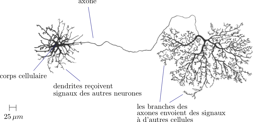
Figure 8.1: Sch ma d’un neurone [Alberts 02]. Le diam tre du corps cellulaire est typiquement de $10\,\mu m$, pendant que la taille des dendrites et des axones varie consid rablement avec la fonction du neurone.

Comme toutes les cellules, les neurones poss dent une diff rence de potentiel entre son cytoplasme et le milieu inter-cellulaire. Cette diff rence de potentiel est contr l e par des m canismes de pompes d’ions, qui peuvent augmenter ou diminuer ce potentiel. Quand la diff rence de potentiel d’un neurone atteint un certain seuil, un m canisme de feedback active les pompes, faisant le potentiel cro tre rapidement jusqu’ environ 100 mV (en d pendant du type de neurone), apr s quoi il atteint la saturation et d cro t, en revenant au potentiel de repos de la cellule. On appelle ce processus un spike.

chaque fois qu’un neurone met un spike, son axone lib re des neurotransmisseurs dans les cellules lesquelles il est connect , en changent leur diff rence de potentiel. Comme les synapses peuvent tre excitatrices ou inhibitrices, les mod les normalement d finissent un poids pour les synapses, avec la convention que un poids positive correspond une synapse qui augmentent le potentiel des neurones auquel elle est connect (et donc favorise les spikes) et un poids n gatif au cas o la synapse d cro t ce potentiel.

Une nouvelle venue de recherche tr s prometteuse dans le domaine des neurosciences a t le d veloppement des techniques d’enregistrement multi-neurones. Dans ces exp riences, une matrice de micro- lectrodes (contant jusqu’ 250 lectrodes) est mise en contact avec le tissu c r bral et le potentiel chaque lectrode est mesur pendant quelques heures. Un proc d sophistiqu d’analyse de donn es permet alors d’identifier la activit individuelle de chaque neurone en contact avec les lectrodes. La sortie typique de un enregistrement multi-neurones est montr e dans la figure suivante.

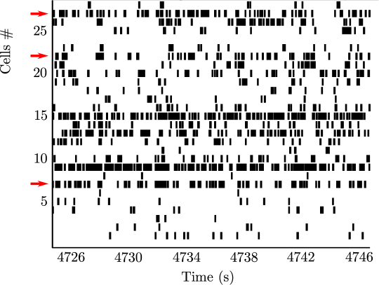
Figure 8.2: R sultat typique d’une exp rience d’enregistrement multi- lectrodes[Peyrache 09]. Chaque ligne correspond un seul neurone, pendant que les barres verticales correspondent des spikes.

En principe, on pourrait trouver les synapses partir des enregistrements multi- lectrodes, mais extraire cet information n’est pas trivial. Na vement, on aurait envie de dire que si l’activit de deux neurones sont corr l es ils sont connect s par une synapse, mais consid rons trois neurones dont l’activit est corr l  : on voit ais ment que toutes les deux configurations montr es dans l’image suivante peut rendre compte des ces corr lations.

Figure 8.3: Deux configurations possibles pour trois neurones corr l s.

Pour pouvoir donner une contribution ce probl me, il est n cessaire d’abord de choisir un mod le pour les r seaux de neurones. Le mod le d’int resse pour cette th se est la machine de Boltzmann [McCulloch 43]. Dans ce mod le, on mod lise l’ tat d’un neurone par une variable binaire : $\sigma=+1$ si il est en train d’ mettre un spike, $\sigma=-1$ sinon. Le r seau de N neurones est alors d crit par un vecteur $\{\sigma_{1},\ldots,\sigma_{N}\}$. Pour simplifier, on ignore totalement la dynamique du syst me et le mod le d crit seulement la probabilit $P(\{\sigma_{1},\ldots,\sigma_{N}\})$ de trouver le syst me dans un tat $\{\sigma_{1},\ldots,\sigma_{N}\}$, qui est donn e par le poids de Boltzmann de un mod le d’Ising g n ralis  :

$$P(\{\sigma_{1},...,\sigma_{N}\}) = \frac{1}{Z}e^{-\beta H(\{\sigma_{1},...,\sigma_{N}\})}\,,$$ (8.1)

avec

$$Z = \sum_{\{\sigma\}}e^{-\beta H(\{\sigma_{1},...,\sigma_{N}\})}\,,$$ (8.2)

o $Z$ est la fonction de partition du mod le, $\beta$ est un param tre du mod le, qui dans le contexte de spins correspond la temp rature inverse et on introduit la notation

$$\sum_{\{\sigma\}}\equiv\sum_{\sigma_{1}=\pm 1}\,\sum_{\sigma_{2}=\pm 1}\,\,\cdots\,\,\sum_{\sigma_{N}=\pm 1}\,.$$ (8.3)

Le Hamiltonien doit prendre en compte les synapses entre les neurones et qu’il doit recevoir une certaine quantit minimum des signaux pour mettre un spike. L’expression la plus utilis e est

$$H(\{\sigma_{1},...,\sigma_{N}\}) = -\frac{1}{2N}\sum_{i,j}J_{ij}\sigma_{i}\sigma_{j}-\sum_{i}h_{i}\sigma_{i}\,,$$ (8.4)

o $J_{ij}$ correspond au poids des synapses et $h_{i}$ est un terme qui mod lise le seuil de spike comme un champs qui attire le neurone vers son tat de repos. Ce mod le est int ressante pour ce travail pour deux raisons : d’abord, il permet de mettre en œuvre directement les outils d velopp s dans le contexte de la m canique statistique et des syst mes d sordonn s. En outre, ce mod le est merge naturellement quand on cherche un mod le qui peut rendre compte d’un ensemble de moyennes $\left\langle\sigma_{i}\right\rangle$ et de corr lations $\left\langle\sigma_{i}\sigma_{j}\right\rangle$. C’est important noter que dans ce mod le les couplages sont sym triques, ie, $J_{ij}=J_{ji}$, ce qui n’est pas forcement vrai dans des syst mes biologiques.

Le mod le d’Ising g n ralis contient comme cas particulier des diff rents mod les classiques de la litt rature. On peut citer le mod le d’Ising ordinaire, le mod le de Sherrington-Kirkpatrick et, d’un int r t particulier pour cette th se, le mod le de Hopfield. Dans ce mod le, le Hamiltonien est donn par

$$H=-\frac{1}{2N}\sum_{\alpha=1}^{p}\left(\sum_{i}\xi_{i}^{\alpha}\sigma_{i}\right)^{2}\,,$$ (8.5)

o $\xi_{i}^{\alpha}$ sont des valeurs r els et en d veloppant le carr on voit bien qu’il correspond au mod le d’Ising g n ralis par

$$J_{ij}=\sum_{\mu=1}^{p}\xi_{i}^{\mu}\xi_{j}^{\mu}\,.$$ (8.6)

L’id e derri re le mod le d’Hopfield est de rendre compte d’un syst me qui garde un nombre $p$ de m moires et peut les retrouver partir d’un tat initial similaire la m moire recherch . Effectivement, dans l’ quation (8.5) on voit bien que si les m moires $\xi^{p}$ sont peu pr s orthogonaux les unes avec les autres, l’ tat $\sigma_{i}=\xi_{i}^{\alpha}$ correspond un minimum local de l’ nergie. Un r sultat classique (voir [Amit 85a]) est que dans certaines conditions, ces tats sont aussi des minimums locales de l’ nergie libre, ce qui permet effectivement de dire que le syst me peut retrouver ces m moires.

D terminer le comportement d’un syst me d crit par un mod le d’Ising g n ralis est normalement tr s difficile et il n’existe pas de solution g n rale pour ce probl me. On peut, par contre, trouver des solutions approch s dans un certain limite de validit . Un cas particulier que nous int resse est le d veloppement en petites couplages introduite par Thouless, Anderson and Palmer (dites quations TAP) [Thouless 77]. Le r sultat qu’ils ont obtenu dit que pour un syst me avec un Hamiltonien donn par

$$H=-\sum_{i<j}J_{ij}\sigma_{i}\sigma_{j}$$ (8.7)

l’ nergie libre est donn e par

$$\log Z = -\sum_{i}\frac{1+m_{i}}{2}\log\left(\frac{1+m_{i}}{2}\right)-\sum_{i}\frac{1-m_{i}}{2}\log\left(\frac{1-m_{i}}{2}\right)$$ (8.8)

$$+\sum_{i<j}J_{ij}m_{i}m_{j}+\frac{1}{2}\sum_{i<j}J_{ij}^{2}(1-m_{i}^{2})(1-m_{j}^{2})+O(J^{3})\,,$$

o $m_{i}=\left\langle\sigma_{i}\right\rangle$ est la magn tisation locale du syst me, qui selon les quations TAP ob issent

$$\tanh^{-1}m_{i} = \sum_{j\,(\neq i)}J_{ij}m_{j}-m_{i}\sum_{j\,(\neq i)}J_{ij}^{2}(1-m_{j}^{2})\,.$$ (8.9)

Malheureusement, dans le cadre des exp riences avec les neurones, on n’a pas besoin d’avoir une m thode pour trouver le comportement d’un syst me en fonction des param tres, mais faire le contraire : trouver les param tres qui rendent compte au mieux des r sultats observ s. On parle alors de “probl mes inverses”.

Travailler avec des probl mes inverses entra ne deux complications suppl mentaires : d’abord, m me pour les cas o on peut r soudre le probl me directe, trouver les param tres qui d crivent les donn es est normalement un probl me difficile. En outre, donner une signification math matique la expression “mieux d crit le syst me” est aussi un point d licat. Une cas possible est que plusieurs diff rents choix de param tres peuvent d crire exactement les mesures. La situation contraire, o il n’existe pas d’ensemble de param tres qui rendent compte des donn es ( cause des erreurs exp rimentaux), est tout aussi possible.

Pour rendre compte de ce probl me, il est utile de postuler que les param tres qui d crivent le probl me suivent eux aussi une loi statistique. On peut alors appliquer le th or me de Bayes qui dit que la probabilit que les param tres valent $\{\lambda_{i}\}$ en fonction des mesures $\{X_{i}\}$ est donn e par

$$P(\{\lambda_{i}\}|\{X_{i}\})=\frac{P(\{X_{i}\}|\{\lambda_{i}\})P_{0}(\{\lambda_{i}\})}{P(\{X_{i}\})}\,,$$ (8.10)

o $P_{0}(\{\lambda_{i}\})$ est la probabilit a priori des param tres et $P(\{X_{i}\})$ est la probabilit marginale de $\{X_{i}\}$, qui peut aussi tre interpr t e comme une normalisation de la probabilit $P(\{\lambda_{i}\}|\{X_{i}\})$ :

$$P(\{X_{i}\})=\sum_{\{\lambda_{i}\}}P(\{X_{i}\}|\{\lambda_{i}\})P_{0}(\{\lambda_{i}\})\,.$$ (8.11)

Ce th or me permet de donner une d finition pr cise du “meilleur” ensemble de param tres pour d crire le syst me comme ceux qui maximisent $P(\{\lambda_{i}\}|\{X_{i}\})$. part cela, s’il existe plus d’un ensemble de param tres qui rendent compte des donn es, un choix judicieux de $P_{0}(\{\lambda_{i}\})$ permet de “choisir” parmi ces solutions et de rendre le probl me bien d finit.

Le probl me d’Ising inverse

On consid re le mod le d’Ising g n ralis avec un Hamiltonien donn par

$$H(\{\sigma_{i}\})=-\sum_{i<j}J_{ij}\,\sigma_{i}\,\sigma_{j}-\sum_{i}h_{i}\,\sigma_{i}\,,$$ (8.12)

qui d finit alors une probabilit sur les tats suivant la loi de Boltzmann

$$P(\{\sigma_{i}\})=\frac{1}{Z}e^{-H(\{\sigma_{i}\})}\,,$$ (8.13)

o $Z$ est la fonction de partition, donn e par

$$Z=\sum_{\{\sigma_{i}\}}e^{-H(\{\sigma_{i}\})}\,.$$ (8.14)

Normalement, quand on tudie un tel syst me on cherche d terminer les magn tisations locales $m_{i}=\left\langle\sigma_{i}\right\rangle$ et les corr lations deux sites $c_{ij}=\left\langle\sigma_{i}\sigma_{j}\right\rangle-m_{i}m_{j}$ en fonction des couplages $\{J_{ij}\}$ et des champs $\{h_{i}\}$. Par contre, on parle de probl me d’Ising inverse quand on cherche d terminer $J_{ij}$ et $h_{i}$ en fonction des corr lations et magn tisations.

Notre point de d part pour r soudre ce probl me est l’entropie de Shannon du probl me

$$S(\{J_{ij}\},\{\lambda_{i}\};\{m_{i}\},\{c_{ij}\})=\log Z(\{J_{ij}\},\{h_{i}\})-\sum_{i<j}J_{ij}\,(c_{ij}+m_{i}\,m_{j})-\sum_{i}h_{i}\,m_{i}\,,\\$$

$$\begin{split}\phantom{xxxx}&=\log\sum_{\{\sigma_{i}\}}\exp\left\{\sum_{i<j}J_{ij}\left[\sigma_{i}\sigma_{j}-c_{ij}-m_{i}m_{j}\right]+\sum_{i}h_{i}(\sigma_{i}-m_{i})\right\}\,,\\ &=\log\sum_{\{\sigma_{i}\}}\exp\left\{\sum_{i<j}J_{ij}\left[(\sigma_{i}-m_{i})(\sigma_{j}-m_{j})-c_{ij}\right]+\sum_{i}\lambda_{i}(\sigma_{i}-m_{i})\right\}\,,\end{split}$$ (8.15)

o on a introduit des nouveaux champs externes $\lambda_{i}$ qui sont li s avec le vrai champs $h_{i}$ par $\lambda_{i}=h_{i}+\sum_{j}J_{ij}\,m_{j}$. On voit ais ment calculant $\partial S/\partial J_{ij}$ et $\partial S/\partial h_{i}$ qui l’ensemble des $J_{ij}^{*}$ et $\lambda_{i}^{*}$ qui reproduisent les magn tisations $m_{i}$ et corr lations $c_{ij}$ est celui qui minimise $S$. On va aussi s’int resser la valeur de $S$ au minimum

$$S(\{m_{i}\},\{c_{ij}\})=\min_{\{J_{ij}\}}\min_{\{\lambda_{i}\}}S(\{J_{ij}\},\{\lambda_{i}\};\{m_{i}\},\{c_{ij}\})\,,$$ (8.16)

car partir de cet expression il est possible d’extraire les valeurs de $J_{ij}^{*}$ et $\lambda_{i}^{*}$ utilisant

$$\frac{\partial S(\{m_{i}\},\{\beta\;c_{ij}\})}{\partial c_{ij}}=-\beta J_{ij}^{*}(\beta)\,,$$ (8.17)

et

$$\frac{\partial S(\{m_{i}\},\{\beta\;c_{ij}\})}{\partial m_{i}}=-\lambda_{i}^{*}(\beta)\,.$$ (8.18)

Comme le probl me d’Ising inverse est tr s difficile r soudre en toute g n ralit , on va chercher une expansion pour des valeurs petites des corr lations. On les multiplie alors toutes pour un param tre $\beta$ qui on introduit, de fa on qu’un expansion en s rie autour de $\beta=0$ correspond une s rie en petites corr lations. L’ quation (8.15) s’ crit alors

$$S(\{J_{ij}\},\{\lambda_{i}\};\{m_{i}\},\{\beta\,c_{ij}\})=\\ =\log\sum_{\{\sigma_{i}\}}\exp\left\{\sum_{i<j}J_{ij}\left[(\sigma_{i}-m_{i})(\sigma_{j}-m_{j})-\beta c_{ij}\right]+\sum_{i}\lambda_{i}(\sigma_{i}-m_{i})\right\}\,.$$ (8.19)

On cherche maintenant trouver une expansion de $S$ au minimum (voir Eq. (8.16)) pour $\beta$ petit :

$$S(\{m_{i}\},\{\beta\,c_{ij}\})=S^{0}+\beta S^{1}+\beta^{2}S^{2}+\ldots\,,$$ (8.20)

d’o on pourra extraire aussi des s ries pour $J_{ij}^{*}$ et $\lambda_{i}^{*}$ utilisant l’ qs. (8.17) et (8.18).

La d termination du premier terme de l’expansion de $S$ est trivial, car quand $\beta=0$ on a des spins d corr l s (qui correspond des spins ind pendants) :

$$S^{0}=-\sum_{i}\left[\frac{1+m_{i}}{2}\ln\frac{1+m_{i}}{2}+\frac{1-m_{i}}{2}\ln\frac{1-m_{i}}{2}\right]\,.$$ (8.21)

Pour trouver les termes non-triviaux de l’entropie, on proc de de la mani re suivante : d’abord, on d finie un potentiel $U$ sur les configurations de spins par (noter le nouveau terme la fin)

$$\begin{split}U(\{\sigma_{i}\})&=\sum_{i<j}J_{ij}^{*}(\beta)\left[(\sigma_{i}-m_{i})(\sigma_{j}-m_{j})-\beta\;c_{ij}\right]+\sum_{i}\lambda_{i}^{*}(\beta)(\sigma_{i}-m_{i})\\ &+\sum_{i<j}c_{ij}\int_{0}^{\beta}\mathrm{\;d}\beta^{\prime}J_{ij}^{*}(\beta^{\prime})\,,\end{split}$$ (8.22)

et une nouvelle entropie ( comparer avec q. (8.15))

$$\tilde{S}(\{m_{i}\},\{c_{ij}\},\beta)=\log\sum_{\{\sigma_{i}\}}e^{U(\{\sigma_{i}\})}\ .$$ (8.23)

Notez que la valeur de $U$ d pends de la valeur des couplages $J_{ij}^{*}(\beta^{\prime})$ tous les valeurs de $\beta^{\prime}<\beta$ et pas seulement pour la valeur de $\beta$ pour laquelle on veux calculer $U$. $S$ et $\tilde{S}$ se relient par

$$S(\{m_{i}\},\{c_{ij}\},\beta)=\tilde{S}(\{m_{i}\},\{c_{ij}\},\beta)-\sum_{i<j}c_{ij}\int_{0}^{\beta}\mathrm{\;d}\beta^{\prime}J_{ij}^{*}(\beta^{\prime})\ .$$ (8.24)

L’expression de $\tilde{S}$ a t choisi de sorte qu’elle soit ind pendante de $\beta$, comme un petit calcul permet de le v rifier

$$\frac{d\tilde{S}}{d\beta}=\frac{\partial\tilde{S}}{\partial\beta}=-\sum_{i<j}c_{ij}\;J_{ij}^{*}(\beta)+\sum_{i<j}c_{ij}\;J_{ij}^{*}(\beta)=0\ .$$ (8.25)

Notez que cela est valable pour toute valeur de $\beta$, d’o $\tilde{S}$ est constante et gal sa valeur en $\beta=0$, $S^{0}$, donn e par l’ q. (8.21).

On utilise alors le fait que $\tilde{S}$ est ind pendant de $\beta$ pour crire des quations d’auto-consistence pour les d riv s de $S$. Par exemple, pour d terminer $S^{1}$, on crit

$$S^{1} = \left.\frac{\partial S}{\partial\beta}\right|_{0}=\left.\frac{\partial\tilde{S}}{\partial\beta}\right|_{0}-\sum_{i<j}c_{ij}J_{ij}^{*}(0)\,,$$ (8.26)

$$= 0\,,$$

o on a utilis que $J_{ij}^{*}(0)=0$ qui d coule du fait que temp rature nulle les spins sont d coupl s.

Pour des ordres plus lev s, on doit proc der ordre par ordre. Pour trouver $S^{k}$ en ayant d j calcul $S^{p}$ pour tout $p<k$, on d marre avec l’ quation $\left.\frac{\partial^{k}\tilde{S}}{\partial\beta^{k}}\right|_{0}=0$, galit cons quence de l’ q. (8.25). Apr s un calcul explicit de la d riv , on se retrouvera avec une quation du type

$$\left.\frac{\partial^{k}\tilde{S}}{\partial\beta^{k}}\right|_{0}=-S^{k}+Q_{k}=0\,,$$ (8.27)

o $Q_{k}$ est une expression qui d pend des magn tisations, corr lations et des d riv s l’ordre $p<k-2$ en z ro des couplages $J_{ij}^{*}$ et des champs $\lambda_{i}^{*}$. En utilisant les qs. (8.17) et (8.18), on peut trouver ces d riv s des couplages et des champs en fonction des valeurs d j connus de $S^{p}$ pour $p<k$ et avoir une expression explicite pour $Q_{k}$ et donc pour $S^{k}$. Le r sultat final pour $S$ est donc

$$S = -\sum_{i}\left[\frac{1+m_{i}}{2}\ln\frac{1+m_{i}}{2}+\frac{1-m_{i}}{2}\ln\frac{1-m_{i}}{2}\right]+\frac{2}{3}\beta^{3}\sum_{i<j}K_{ij}^{3}m_{i}m_{j}L_{i}L_{j}$$ (8.28)

$$+\frac{\beta^{4}}{6}\sum_{i<j}K_{ij}^{4}\left[1-3m_{i}^{2}-3m_{j}^{2}-3m_{i}^{2}m_{j}^{2}\right]L_{i}L_{j}$$

$$-\frac{\beta^{2}}{2}\sum_{i<j}K_{ij}^{2}L_{i}L_{j}+\beta^{3}\sum_{i<j<k}K_{ij}K_{jk}K_{ki}L_{i}L_{j}L_{k}$$

$$-\frac{\beta^{4}}{8}\sum_{i,j,k,l}K_{ij}K_{jk}K_{kl}K_{li}L_{i}L_{j}L_{k}L_{l}$$

$$+O(\beta^{5})\,.$$

Les couplages sont donn es par

$$J_{ij}^{*}(\{c_{kl}\},\{m_{i}\},\beta) = \beta K_{ij}-2\beta^{2}m_{i}m_{j}K_{ij}^{2}-\beta^{2}\sum_{k}K_{jk}K_{ki}L_{k}$$ (8.29)

$$+\frac{1}{3}\beta^{3}K_{ij}^{3}\left[1+3m_{i}^{2}+3m_{j}^{2}+9m_{i}^{2}m_{j}^{2}\right]$$

$$+\beta^{3}\sum_{\begin{subarray}{c}k\\ (\neq i,\,\neq j)\end{subarray}}K_{ij}(K_{jk}^{2}L_{j}+K_{ki}^{2}L_{i})L_{k}$$

$$+\beta^{3}\sum_{\begin{subarray}{c}k,l\\ (k\neq i,\,l\neq j)\end{subarray}}K_{jk}K_{kl}K_{li}L_{k}L_{l}+O(\beta^{4})\,,$$

et le champs $h$ par

$$h_{l}^{*}(\{c_{ij}\},\{m_{i}\},\beta) = \frac{1}{2}\ln\left(\frac{1+m_{l}}{1-m_{l}}\right)-\sum_{j}J_{lj}^{*}m_{j}+\beta^{2}\sum_{j(\neq l)}K_{lj}^{2}m_{l}L_{j}$$ (8.30)

$$-\frac{2}{3}\beta^{3}(1+3m_{l}^{2})\sum_{j(\neq l)}K_{lj}^{3}m_{j}L_{j}-2\beta^{3}m_{l}\sum_{j<k}K_{lj}K_{jk}K_{kl}L_{j}L_{k}$$

$$+2\beta^{4}m_{l}\sum_{i<j}\sum_{k}K_{ik}K_{kj}K_{jl}K_{li}L_{i}L_{j}L_{k}$$

$$+\beta^{4}m_{l}\sum_{j}K_{lj}^{4}L_{j}\left[1+m_{l}^{2}+3m_{j}^{2}+3m_{l}^{2}m_{j}^{2}\right]$$

$$+\beta^{4}m_{l}\sum_{i\,(\neq l)}\sum_{j}K_{ij}^{2}K_{jl}^{2}L_{i}L_{j}^{2}+O(\beta^{5})\,.$$

Dans ces expressions on a utilis les notations

$$L_{i}=\left\langle\left(\sigma_{i}-m_{i}\right)^{2}\right\rangle_{0}=1-m_{i}^{2}\,,$$ (8.31)

qui est la d viation standard d’un spin ind pendant $m_{i}$ et

$$K_{ij}=\delta_{ij}\frac{\left\langle\left(\sigma_{i}-m_{i}\right)\left(\sigma_{j}-m_{j}\right)\right\rangle_{0}}{\left\langle\left(\sigma_{i}-m_{i}\right)^{2}\right\rangle_{0}\left\langle\left(\sigma_{j}-m_{j}\right)^{2}\right\rangle_{0}}=\delta_{ij}\frac{c_{ij}}{L_{i}L_{j}}\,,$$ (8.32)

o $\delta_{ij}$ est le symbole de Kronecker.

Malheureusement, on a v rifi que la qualit d’inf rence obtenue par cette formule se d grade tr s rapidement quand on sort de son limite de validit $c_{ij}\ll 1$. Pour am liorer son stabilit , on a remarqu que les trois derniers termes de l’ q. (8.28) peuvent s’ crire de la forme d’une s rie altern

$$-\frac{\beta^{2}}{4}\operatorname*{Tr}(M^{2})+\frac{\beta^{3}}{6}\operatorname*{Tr}(M^{3})-\frac{\beta^{4}}{8}\operatorname*{Tr}(M^{4})\,,$$ (8.33)

o $M$ est la matrice d finit par $M_{ij}=K_{ij}\sqrt{L_{i}L_{j}}$. Comme $K_{ii}=0$, on a que $\operatorname*{Tr}{M}=0$, donc les trois derniers termes s’ crivent

$$S^{\text{loop}} = \frac{1}{2}\operatorname*{Tr}\left(\beta M-\frac{\beta^{2}}{2}M^{2}+\frac{\beta^{3}}{3}M^{3}-\frac{\beta^{4}}{4}M^{4}\right)$$ (8.34)

$$= \operatorname*{Tr}\left[\log(1+\beta M)\right]+O(\beta^{5})$$

$$= \log\left[\det(1+\beta M)\right]+O(\beta^{5})$$

Cette expression peut aussi tre retrouv e comme une cons quence de l’ q. (8.9), ce qui montre qu’elle correspond une approximation du type “champs moyen” de l’entropie. En outre, si on remplace les trois derniers termes de l’ q. (8.28) par cette expression, on voit une nette am lioration de la stabilit de l’inf rence. Cela s’explique car tr s probablement les termes d’ordre sup rieure $O(\beta^{5})$ du d veloppement de $\log[\det(1+\beta M)]$ sont contenus dans l’expansion de $S$, et les d velopper en s rie correspond une s rie altern e, divergente pour des valeurs mod r ment grands de $c_{ij}$.

Comme l’expression de champs moyen a pu am liorer consid rablement la stabilit de l’expansion, on a cherch int grer une autre approximation possible du probl me : l’approximation de pairs ind pendants, dans laquelle on examine chaque pair de sites $i$ et $j$ comme un syst me compos de juste deux spins. Utilisant cette expression et l’approximation de champs moyen d crite dans le paragraphe pr c dant, on obtient

$$S^{\text{2-spin + loop}} = \sum_{i}S^{\text{1-spin}}_{i}+\sum_{i<j}\left[S_{ij}^{\text{2-spin}}-S^{\text{1-spin}}_{i}-S^{\text{1-spin}}_{j}\right]$$ (8.35)

$$+S^{\text{loop}}-\frac{1}{2}\sum_{i<j}\log(1-K_{ij}^{2}L_{i}L_{j})\,.$$

o

$$S^{\text{2-spin}}_{ij} = S^{\text{1-spin}}_{i}+S^{\text{1-spin}}_{j}$$ (8.36)

$$+\frac{1}{4}\log\left[1+\frac{c_{ij}}{(1-m_{i})(1-m_{j})}\right][c_{ij}+(1-m_{i})(1-m_{j})]$$

$$+\frac{1}{4}\log\left[1-\frac{c_{ij}}{(1-m_{i})(1+m_{j})}\right][c_{ij}-(1-m_{i})(1+m_{j})]$$

$$+\frac{1}{4}\log\left[1-\frac{c_{ij}}{(1+m_{i})(1-m_{j})}\right][c_{ij}-(1+m_{i})(1-m_{j})]$$

$$+\frac{1}{4}\log\left[1+\frac{c_{ij}}{(1+m_{i})(1+m_{j})}\right][c_{ij}+(1+m_{i})(1+m_{j})]\,,$$

et

$$S^{\text{1-spin}}_{i} = -\left[\frac{1+m_{i}}{2}\ln\frac{1+m_{i}}{2}+\frac{1-m_{i}}{2}\ln\frac{1-m_{i}}{2}\right]\,.$$ (8.37)

Cette expression est quivalente l’ q. (8.28) (ils ne diff rent que en termes d’ordre $O(\beta^{5})$ ou plus), mais elle est beaucoup plus stable num riquement. La formule pour $J_{ij}^{*}$ qui se d duit de cette expression est

$$J_{ij}^{*(\text{2-spin+loop})} = J_{ij}^{*\text{loop}}+J_{ij}^{*\text{2-spin}}-\frac{K_{ij}}{1-K_{ij}^{2}L_{i}L_{j}}\,,$$ (8.38)

o

$$J_{ij}^{*(\text{2-spin})} = \phantom{+}\frac{1}{4}\ln\left[1+K_{ij}(1+m_{i})(1+m_{j})\right]$$ (8.39)

$$+\frac{1}{4}\ln\left[1+K_{ij}(1-m_{i})(1-m_{j})\right]$$

$$-\frac{1}{4}\ln\left[1-K_{ij}(1-m_{i})(1+m_{j})\right]$$

$$-\frac{1}{4}\ln\left[1-K_{ij}(1+m_{i})(1-m_{j})\right]$$

et

$$J_{ij}^{\text{loop}} = \frac{1}{\sqrt{(1-m_{i}^{2})(1-m_{j}^{2})}}\left[M(M+1)^{-1}\right]_{ij}\,.$$ (8.40)

Inf rence d’un mod le de Hopfield

Dans la partie pr c dente, on s’est int ress un mod le d’Ising g n ralis sans pr ciser la forme des couplages. Maintenant, on s’int resse au cas particulier d’un mod le de Hopfield. Il y a plusieurs avantages d’utiliser ce mod le : d’abord, il existe d’exp riences de enregistrement multi-neurones o on ne cherche pas trouver des couplages entre les neurones mais d’en extraire des patterns. Deuxi mement, on s’attend que diminuer le nombre de d gr es de libert du probl me rends la proc dure d’inf rence plus stable. Finalement, le mod le de Hopfield peut tre r solu analytiquement, d’o on esp re avoir un meilleur contr le des erreurs d’inf rence.

Notez qu’en principe on pourrais proc der par d’abord inf rer la matrice $\{J_{ij}\}$ des couplages pour ensuite la diagonaliser pour trouver un ensemble de patterns. Le probl me de cette approche est qu’elle n’est pas optimale d’un point de vue Bayesian : les patterns trouv s ne seront pas forcement ceux qui maximisent la probabilit a posteriori. Cela est particuli rement probl matique quand la supposition de que le syst me qu’on tude est d crit par un mod le de Hopfield est juste une approximation.

Dans cette partie on va avoir deux buts : premi rement, on va chercher une formule permettant d’inf rer les patterns en fonction des donn es. Ensuite, on va s’int resser estimer le nombre de fois qu’on doit mesurer le syst me pour avoir une bonne inf rence.

Premi rement, on remarque que trouver les patterns qui mieux rendent compte d’une s quence de donn es est un probl me mal pos , car il y a plusieurs ensembles de patterns qui peuvent d crire le m me syst me. Supposons pour exemple le cas de deux patterns ($p=2$) :

$$H=N\left(\frac{1}{N}\sum_{i}\xi_{i}^{1}\sigma_{i}\right)^{2}+N\left(\frac{1}{N}\sum_{i}\xi_{i}^{2}\sigma_{i}\right)^{2}\,.$$ (8.41)

Si l’on d finit un nouveau ensemble de patterns donn e par $\tilde{\xi_{i}^{1}}=\xi_{i}^{1}\cos\theta+\xi_{i}^{2}\sin\theta$ et $\tilde{\xi_{i}^{2}}=-\xi_{i}^{1}\sin\theta+\xi_{i}^{2}\cos\theta$, le nouveau Hamiltonien est

$$\tilde{H} = N\left[\frac{1}{N}\sum_{i}(\xi_{i}^{1}\cos\theta+\xi_{i}^{2}\sin\theta)\sigma_{i}\right]^{2}$$ (8.42)

$$+N\left[\frac{1}{N}\sum_{i}(-\xi_{i}^{1}\sin\theta+\xi_{i}^{2}\cos\theta)\sigma_{i}\right]^{2}\,,$$

$$= H\,.$$ (8.43)

En g n rale, si on a $p$ patterns, faire une rotation des patterns en $p$ dimensions ne change pas le Hamiltonien du syst me. On dit que le syst me poss de une invariance de gauge. Alors, pour rendre le probl me d’inf rence bien pos e on doit soit lever cette d g n rescence en additionnant des contraintes pour lever les $p(p-1)/2$ d gr es de libert , soit additionner un prior $P_{0}$ dans notre probabilit Bayesienne. Pour des raisons techniques, on va se concentrer sur la premi re solution.

Pour pouvoir d velopper un m thode d’inf rence, il est n cessaire de traiter s par ment le cas o le syst me est dans une phase ferromagn tique et le cas d’une phase paramagn tique. Dans le premier cas, on va supposer que les donn es qu’on dispose pour faire l’inf rence sont des mesures des configurations du syst me. On suppose de plus que ces mesures sont une r alisation de la loi de Boltzmann. Comme les minimums de l’ nergie libre correspondent des configurations magn tis s selon un des patterns[Amit 85a], on suppose qu’on a mesur $l_{1}$ configurations magn tis s selon le premier pattern, $l_{2}$ selon le deuxi me et ainsi de suite. Dans ce cas, si on estime partir des mesures la corr lation entre deux sites, on a

$$C_{ij} = \frac{1}{L}\sum_{l}\sigma_{i}^{l}\sigma_{j}^{l}$$ (8.44)

$$= \sum_{k=1}^{p}\frac{1}{L}\sum_{l\in l_{k}}\sigma_{i}^{l}\sigma_{j}^{l}$$

$$\approx \frac{1}{L}\sum_{k=1}^{p}l_{k}m_{i}^{k}m_{j}^{k}+O(1/N)\,,$$

o

$$m^{k} = \frac{1}{N}\sum_{i}\xi_{i}^{k}\tanh(m_{k}\xi_{i}^{k})\,,$$ (8.45)

et

$$m^{k}_{i} = \tanh(m^{k}\xi_{i}^{k})\,,$$ (8.46)

d’o on peut ais ment inf rer les patterns en diagonalisant la matrice $C_{ij}$. Notez que cette proc dure choisi implicitement un gauge tel que

$$\sum_{i}\tanh(m^{k}\xi_{i}^{k})\tanh(m^{k^{\prime}}\xi_{i}^{k^{\prime}})=0,\quad\text{avec $k\neq k^{\prime}$}\,.$$ (8.47)

Le cas paramagn tique est plus int ressant, mais plus complexe. D’abord, comme on cherche un syst me dans une phase o il n’est pas magn tis selon aucun pattern, on suppose qu’il existe un champs externe suffisamment fort pour que les magn tisations $m_{i}$ soit domin es par le champs externe locale $h_{i}$. Aussi, pour faciliter les calculs qui suivent, on remplace le Hamiltonien habituel du mod le d’Hopfield ( q. (8.5)) par

$$H=-\frac{1}{N}\sum_{\mu=1}^{p}\sum_{i<j}\xi_{i}^{\mu}\xi_{j}^{\mu}(\sigma_{i}-\tanh h_{i})(\sigma_{j}-\tanh h_{j})-\sum_{i}h_{i}\sigma_{i}\,.$$ (8.48)

Ce Hamiltonien permet de retrouver l’ q. (8.5) par une translation du champs externe :

$$h_{i}\rightarrow h_{i}-\sum_{\mu}\sum_{j\,(\neq i)}\xi_{i}^{\mu}\xi_{j}^{\mu}\tanh h_{j}\,.$$ (8.49)

Utilisant le th or me de Bayes (eq. (8.10)), on a alors

$$\begin{split}P(\{\xi_{i}^{\mu}\}&|\{\sigma^{l}\})=\frac{P_{0}(\{\xi_{i}^{\mu}\})}{Z(\{\xi_{i}^{\mu}\})^{L}P(\{\sigma^{l}\})}\times\\ &\times\prod_{l=1}^{L}\exp\left[\frac{\beta}{N}\sum_{\mu=1}^{p}\sum_{i<j}\xi_{i}^{\mu}\xi_{j}^{\mu}(\sigma_{i}^{l}-\tanh h_{i})(\sigma_{j}^{l}-\tanh h_{j})+\beta\sum_{i}h_{i}\sigma_{i}^{l}\right]\,.\end{split}$$ (8.50)

On voit que cette probabilit ne d pend que des valeurs mesur s des corr lations et magn tisations

$$m_{i}=\frac{1}{L}\sum_{l}\sigma_{i}^{l}\,,\quad\quad c_{ij}=\frac{1}{L}\sum_{l}\sigma_{i}^{l}\sigma_{j}^{l}-m_{i}m_{j}\,,$$ (8.51)

donnant

$$\begin{split}P(\{\xi_{i}^{\mu}\}|&\{\sigma^{l}\})=\frac{P_{0}(\{\xi_{i}^{\mu}\})}{Z(\{\xi_{i}^{\mu}\})^{L}P(\{\sigma^{l}\})}\exp\Bigg{[}\frac{\beta L}{N}\sum_{\mu=1}^{p}\sum_{i<j}\xi_{i}^{\mu}\xi_{j}^{\mu}c_{ij}\\ &+\frac{\beta L}{N}\sum_{\mu}\sum_{i<j}\xi_{i}^{\mu}\xi_{j}^{\mu}(m_{i}-\tanh h_{i})(m_{j}-\tanh h_{j})+\beta L\sum_{i}h_{i}m_{i}\Bigg{]}\,.\end{split}$$ (8.52)

Pour optimiser cette quantit par rapport aux patterns $\xi_{i}^{\mu}$, il est n cessaire d’ crire explicitement un d veloppement de $\log Z$ pour $N$ grand, ce qui est fait dans l’Appendice D. La minimisation en soit tant assez technique, elle peut tre consult au chapitre 6. Le r sultat final, l’ordre dominante en $N$, est

$$h_{i}^{0} = \tanh^{-1}m_{i}\,.$$ (8.53)

et

$$\xi_{i}^{\mu,0}=\sqrt{1-\frac{1}{\lambda_{\mu}}}\frac{v_{i}^{\mu}}{\sqrt{1-\tanh^{2}h_{i}^{0}}}\,,$$ (8.54)

o $\lambda_{\mu}$ et $v^{\mu}$ sont, respectivement, le $\mu$- me plus grande valeur propre de la matrice $M$ et sont vecteur propre associ , o $M$ est donn e par

$$M_{ij}=\frac{c_{ij}}{\sqrt{1-\tanh^{2}h_{i}^{0}}\sqrt{1-\tanh^{2}h_{j}^{0}}}\,.$$ (8.55)

C’est int ressant de noter que cette expression implique que

$$J_{ij} = \sum_{\alpha}\frac{\lambda_{\alpha}-1}{\lambda_{\alpha}}\frac{v_{i}^{\alpha}v_{j}^{\alpha}}{\sqrt{(1-m_{i}^{2})(1-m_{j}^{2})}}$$ (8.56)

$$= \frac{1}{\sqrt{(1-m_{i}^{2})(1-m_{j}^{2})}}\left[M^{-1}(M-1)\right]_{ij}\,,$$

qui est exactement l’expression d j trouv e dans l’ q. (8.40) pour le mod le d’Ising g n ralis .

Dans le but de trouver une expression in dite pour l’inf rence, on a aussi d termin les corrections sous-dominantes correspondant l’ q. (8.54). Les d tails se trouvent dans le chapitre 6. Malheureusement, l’expression trouv e est tr s sensible des erreurs al atoires sur les magn tisations et corr lations mesur es, donc peu utile pour des donn es r els.

Un autre probl me int ressant est de savoir combien de mesures on doit faire d’un syst me d’Hopfield pour qu’il soit possible d’inf rer pr cis ment les valeurs de ses patterns. Pour donner une r ponse ce probl me, on a calcul l’entropie de Shannon de la proc dure d’inf rence, car il est raisonnable de penser que quand $S/N\ll 1$, on peut trouver les patterns avec un erreur faible. On rappelle que l’entropie de Shannon d’une distribution de probabilit $P$ d fini sur un ensemble $\Omega$ est

$$S=-\sum_{\omega\in\Omega}P(\omega)\log P(\omega)\,.$$ (8.57)

Dans le cas de notre inf rence, la probabilit est donn par le th or me de Bayes (eq. (8.10)) et on suppose que nos patterns ne peuvent valoir que $\pm\sqrt{\beta}$, o $\beta$ est une constante fixe, qu’on associe une temp rature inverse. On traite d’abord le cas d’un seul pattern. On a alors

$$S[\{\sigma_{i}^{l}\}] = -\frac{1}{\mathcal{N}[\{\sigma_{i}^{l}\}]Z(\beta)^{L}}\sum_{\{\xi\}}\exp\left(\frac{\beta}{N}\sum_{l=0}^{L}\sum_{i<j}\xi_{i}\xi_{j}\sigma_{i}^{l}\sigma_{j}^{l}\right)\times$$ (8.58)

$$\times\left[-\log\left(\mathcal{N}[\{\sigma_{i}^{l}\}]Z(\beta)^{L}\right)+\left(\frac{\beta}{N}\sum_{l=0}^{L}\sum_{i<j}\xi_{i}\xi_{j}\sigma_{i}^{l}\sigma_{j}^{l}\right)\right]\,.$$

o

$$\mathcal{N}[\{\sigma_{i}^{l}\}]=Z(\beta)^{-L}\sum_{\{\xi\}}\exp\left(\frac{\beta}{N}\sum_{l=0}^{L}\sum_{i<j}\xi_{i}\xi_{j}\sigma_{i}^{l}\sigma_{j}^{l}\right)\,.$$ (8.59)

Notez que $S$ d pend explicitement des mesures $\{\sigma_{i}\}$. Par contre, il est naturel d’esp rer que pour un syst me assez grand et pour un nombre pas trop petit de mesures, l’entropie va d pendre plus des caract ristiques du syst me que des d tail des mesures effectu es. On s’int resse alors calculer $\left\langle S\right\rangle$, o la moyenne est effectu par rapport la probabilit de Boltzmann de mesurer les configurations $\{\sigma_{i}\}$, en supposant que le syst me que les a g n r est d crit par un mod le de Hopfield.

Le comportement de $\left\langle S\right\rangle$ est tr s diff rent pour les deux phases du syst me. S’il est dans une phase ferromagn tique, l’entropie d croit exponentiellement avec le nombre de mesures $L$. On peut trouver les d tails du calcul et l’expression analytique de l’entropie dans le chapitre 7. Les r sultats sont repr sent s dans le graphique suivant :

Figure 8.4: Entropie par spin en fonction du nombre de mesures $L$ pour $\beta=1.1$. Notez le comportement asymptotique $\left\langle S\right\rangle\approx Ce^{\gamma L}$ o $\gamma=\log\cosh(\beta m)$.

Ce r sultat montre que le nombre de mesures n cessaires pour inf rer le pattern du syst me est une grandeur intensive du syst me, ie, il reste finit quand la taille du syst me tends vers l’infini.

Quand le syst me est dans la phase paramagn tique, cette situation se modifie. En fait, il faut un nombre de mesures $L=\alpha N$ proportionnel la taille du syst me pour pouvoir inf rer le pattern. Comme on peut voir dans le chapitre 7, les calculs sont aussi plus complexes, et on est oblig d’utiliser des m thodes des syst mes d sordonn es (notamment la m thode des r pliques) pour trouver une expression analytique pour l’entropie moyenne. Un graphique illustrant les r sultats obtenus se trouve dans la Fig. 8.5.

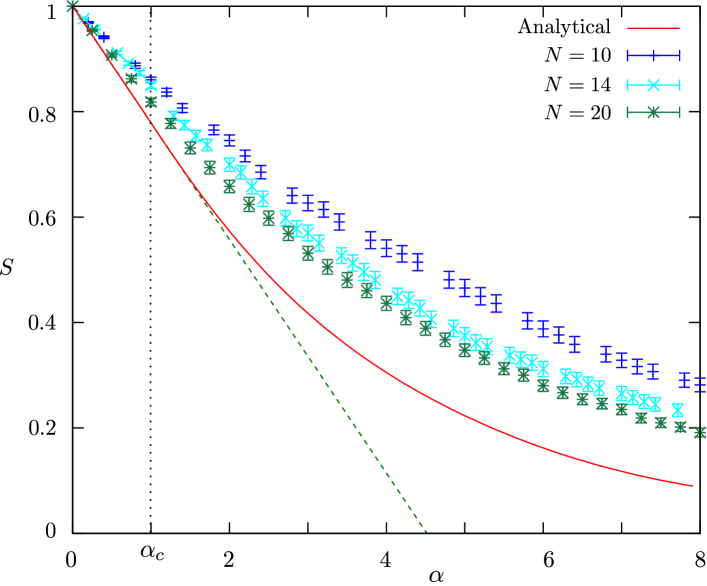
Figure 8.5: Entropie par spin comme fonction de $\alpha$ pour $\beta=0.5$. La ligne solide correspond la solution analytique trouv dans le chapitre 7 et les points correspondent des r sultats num riques.

Finalement, pour le cas de plusieurs patterns dans la phase paramagn tique, on retrouve que l’entropie de l’inf rence de chaque pattern d croit comme l’entropie du syst me o on n’a qu’un seul pattern (Fig. 8.5).

Appendix A Details of the small-$\bm{\beta}$ expansion

Let $O$ be an observable of the spin configuration (which can explicitly depend on the inverse temperature $\beta$), and

$$\left\langle O\right\rangle=\frac{1}{Z}\sum_{\{\sigma\}}O(\{\sigma\})\;e^{U(\{\sigma\})}$$ (A.1)

its average value, where $U$ is defined in (4.13), and $Z=\exp(\tilde{S})$. The derivative of the average value of $O$ fulfills the following identity,

$$\frac{\partial\left\langle O\right\rangle}{\partial\beta}=\frac{1}{Z}\sum_{\{\sigma\}}\left[\frac{\partial O}{\partial\beta}+O\frac{\partial U}{\partial\beta}\right]e^{U}-\frac{1}{Z^{2}}\frac{\partial Z}{\partial\beta}\sum_{\{\sigma\}}Oe^{U}=\left\langle\frac{\partial O}{\partial\beta}\right\rangle+\left\langle O\frac{\partial U}{\partial\beta}\right\rangle$$ (A.2)

where the term in $Z^{-2}$ vanishes as a consequence of (4.16).

A.1 Second order expansion

Using (A.2) and (4.21)

$$0=\frac{\partial^{3}\tilde{S}}{\partial\beta^{3}}=\frac{\partial}{\partial\beta}\left[\left\langle\frac{\partial^{2}U}{\partial\beta^{2}}\right\rangle+\left\langle\left(\frac{\partial U}{\partial\beta}\right)^{2}\right\rangle\right]=\left\langle\frac{\partial^{3}U}{\partial\beta^{3}}\right\rangle+3\left\langle\frac{\partial^{2}U}{\partial\beta^{2}}\frac{\partial U}{\partial\beta}\right\rangle+\left\langle\left(\frac{\partial U}{\partial\beta}\right)^{3}\right\rangle$$ (A.3)

A straightforward calculation gives (where we omit for clarity the notation $|_{0}$ and the ^∗ subscript from $J_{ij}$ and $\lambda_{i}$)

$$\left\langle\frac{\partial^{3}U}{\partial\beta^{3}}\right\rangle_{0} = -2\sum_{i<j}\frac{\partial^{2}J_{ij}}{\partial\beta^{2}}c_{ij}$$ (A.4)

$$\left\langle\frac{\partial^{2}U}{\partial\beta^{2}}\frac{\partial U}{\partial\beta}\right\rangle_{0} = \sum_{i<j}\frac{\partial^{2}J_{ij}}{\partial\beta^{2}}\frac{\partial J_{ij}}{\partial\beta}L_{i}L_{j}+\sum_{i}\frac{\partial^{2}\lambda_{i}}{\partial\beta^{2}}\frac{\partial\lambda_{i}}{\partial\beta}L_{i}$$ (A.5)

$$\left\langle\left(\frac{\partial U}{\partial\beta}\right)^{3}\right\rangle_{0} = 6\sum_{i<j<k}\frac{\partial J_{ij}}{\partial\beta}\frac{\partial J_{jk}}{\partial\beta}\frac{\partial J_{ki}}{\partial\beta}L_{i}L_{j}L_{k}+$$ (A.6)

$$+ \sum_{i<j}\left(\frac{\partial J_{ij}}{\partial\beta}\right)^{3}4m_{i}m_{j}L_{i}L_{j}+6\sum_{i<j}\frac{\partial J_{ij}}{\partial\beta}\frac{\partial\lambda_{i}}{\partial\beta}\frac{\partial\lambda_{j}}{\partial\beta}L_{i}L_{j}$$

Using (A.3), the expressions of the derivatives of $\lambda_{i}$ in $\beta=0$, we obtain

$$Q_{2}=-4\sum_{i<j}\frac{c_{ij}^{3}m_{i}m_{j}}{(1-m_{i}^{2})^{2}(1-m_{j}^{2})^{2}}-6\sum_{i<j<k}\frac{c_{ij}c_{jk}c_{ki}}{(1-m_{i}^{2})(1-m_{j}^{2})(1-m_{k}^{2})}$$ (A.7)

from which we deduce

$$\left.\frac{\partial^{3}S}{\partial\beta^{3}}\right|_{0}=4\sum_{i<j}K_{ij}^{3}m_{i}m_{j}L_{i}L_{j}+6\sum_{i<j<k}K_{ij}K_{jk}K_{ki}L_{i}L_{j}L_{k}$$ (A.8)

and

$$\left.\frac{\partial^{2}J_{ij}}{\partial\beta^{2}}\right|_{0}=-4m_{i}m_{j}K_{ij}^{2}-2\sum_{k(\neq i,\,\neq j)}K_{jk}K_{ki}L_{k}\ .$$ (A.9)

A.2 Third order expansion

The procedure to derive the third order expansion for the coupling is identical to the second order one. We start from

$$0=\frac{\partial^{4}\tilde{S}}{\partial\beta^{4}}=\left\langle\frac{\partial^{4}U}{\partial\beta^{4}}\right\rangle+3\left\langle\left(\frac{\partial^{2}U}{\partial\beta^{2}}\right)^{2}\right\rangle+4\left\langle\frac{\partial^{3}U}{\partial\beta^{3}}\frac{\partial U}{\partial\beta}\right\rangle+6\left\langle\left(\frac{\partial U}{\partial\beta}\right)^{2}\frac{\partial^{2}U}{\partial\beta^{2}}\right\rangle+\left\langle\left(\frac{\partial U}{\partial\beta}\right)^{4}\right\rangle$$ (A.10)

and evaluate each term in the sum:

$$\left\langle\frac{\partial^{4}U}{\partial\beta^{4}}\right\rangle_{0} = -3\sum_{i<j}\left.\frac{\partial^{3}J_{ij}}{\partial\beta^{3}}\right|_{0}K_{ij}L_{i}L_{j}$$ (A.11)

$$\left\langle\left(\frac{\partial^{2}U}{\partial\beta^{2}}\right)^{2}\right\rangle_{0} = \sum_{i<j}\left(\frac{\partial^{2}J_{ij}}{\partial\beta^{2}}\right)^{2}L_{i}L_{j}+\sum_{i}\left(\frac{\partial^{2}\lambda_{i}}{\partial\beta^{2}}\right)^{2}L_{i}+\left[\sum_{i<j}K_{ij}^{2}L_{i}L_{j}\right]^{2}$$ (A.12)

$$\left\langle\frac{\partial^{3}U}{\partial\beta^{3}}\frac{\partial U}{\partial\beta}\right\rangle_{0} = \sum_{i<j}K_{ij}\frac{\partial^{3}J_{ij}}{\partial\beta^{3}}L_{i}L_{j}$$ (A.13)

$$\left\langle\left(\frac{\partial U}{\partial\beta}\right)^{2}\frac{\partial^{2}U}{\partial\beta^{2}}\right\rangle_{0} = 2\sum_{i<k}\sum_{j}K_{ij}K_{jk}\frac{\partial^{2}J_{ki}}{\partial\beta^{2}}L_{i}L_{j}L_{k}+4\sum_{i<j}K_{ij}^{2}\frac{\partial^{2}J_{ij}}{\partial\beta^{2}}m_{i}m_{j}L_{i}L_{j}$$ (A.14)

$$+ \sum_{i}\sum_{j}K_{ij}^{2}\frac{\partial^{2}\lambda_{i}}{\partial\beta^{2}}(-2m_{i})L_{i}L_{j}-\left\langle\left(\frac{\partial U}{\partial\beta}\right)^{2}\right\rangle_{0}\sum_{i<j}K_{ij}^{2}L_{i}L_{j}$$

$$\left\langle\left(\frac{\partial U}{\partial\beta}\right)^{4}\right\rangle_{0} = \sum_{i<j}K_{ij}^{4}(3m_{i}^{2}+1)L_{i}(3m_{j}^{2}+1)L_{j}+3\sum_{i<j,\,k<l\,(k\neq i,\,l\neq j)}K_{ij}^{2}K_{kl}^{2}L_{i}L_{j}L_{k}L_{l}+$$ (A.15)

$$+ 6\sum_{i<k}\sum_{j}K_{ij}^{2}K_{jk}^{2}(3m_{j}^{2}+1)L_{i}L_{j}L_{k}+$$

$$+ 12\sum_{i<j<k}K_{ij}K_{jk}K_{ki}L_{i}L_{j}L_{k}\left[4m_{i}m_{j}K_{ij}+4m_{i}m_{k}K_{ik}+4m_{k}m_{i}K_{ki}\right]+$$

$$+ 3\sum_{i,j,k,l\,(\neq)}K_{ij}K_{jk}K_{kl}K_{li}L_{i}L_{j}L_{k}L_{l}$$

Using the results of Eq. (4.9) and (4.10) we can write all the terms above in the same form

$$-3\left[\sum_{i<j}K_{ij}^{2}L_{i}L_{j}\right]^{2} = -3\sum_{i<j,\,k<l\,(k\neq i,\,l\neq j)}K_{ij}^{2}K_{kl}^{2}L_{i}L_{j}L_{k}L_{l}$$ (A.16)

$$-6\sum_{i<j}\sum_{k}K_{ik}^{2}K_{kj}^{2}L_{i}L_{j}L_{k}^{2}$$

$$-3\sum_{i<j}K_{ij}^{4}L_{i}^{2}L_{j}^{2}$$

$$12\sum_{i<j}\sum_{k}K_{ik}K_{kj}\frac{\partial^{2}J_{ij}}{\partial\beta^{2}}L_{i}L_{j}L_{k} = -48\sum_{i<j}\sum_{k}K_{ij}^{2}K_{ik}K_{kj}m_{i}m_{j}L_{i}L_{j}L_{k}-$$ (A.17)

$$-12\sum_{i,j,k,l\,(\neq)}K_{ij}K_{jk}K_{kl}K_{li}L_{i}L_{j}L_{k}L_{l}$$

$$-24\sum_{i<j}\sum_{k}K_{ik}^{2}K_{kj}^{2}L_{i}L_{j}L_{k}^{2}$$

$$\sum_{i<j}K_{ij}^{2}\frac{\partial^{2}J_{ij}}{\partial\beta^{2}}m_{i}m_{j}L_{i}L_{j} = -4\sum_{i<j}K_{ij}^{4}m_{i}^{2}m_{j}^{2}L_{i}L_{j}$$ (A.18)

$$-2\sum_{i<j}\sum_{k}K_{ij}^{2}K_{jk}K_{ki}m_{i}m_{j}L_{i}L_{j}L_{k}$$

$$3\sum_{i<j}\left(\frac{\partial^{2}J_{ij}}{\partial\beta^{2}}\right)^{2}L_{i}L_{j} = 48\sum_{i<j}K_{ij}^{4}m_{i}^{2}m_{j}^{2}L_{i}L_{j}+$$ (A.19)

$$48\sum_{i<j}\sum_{k}K_{ij}^{2}K_{ik}K_{kj}m_{i}m_{j}L_{i}L_{j}L_{k}+$$

$$+6\sum_{i,j,k,l\,(\neq)}K_{ij}K_{jk}K_{kl}K_{li}L_{i}L_{j}L_{k}L_{l}$$

$$+12\sum_{i<j}\sum_{k}K_{ik}^{2}K_{kj}^{2}L_{k}^{2}L_{i}L_{j}$$

$$6\sum_{i}\sum_{j}K_{ij}^{2}\frac{\partial^{2}\lambda_{i}}{\partial\beta^{2}}(-2m_{i})L_{i}L_{j} = -24\sum_{i}\sum_{j}K_{ij}^{4}m_{i}^{2}(1-m_{j}^{2})L_{i}L_{j}$$ (A.20)

$$-48\sum_{i<j}\sum_{k}K_{ik}^{2}K_{kj}^{2}m_{k}^{2}L_{i}L_{j}L_{k}$$

$$3\sum_{k}\left(\frac{\partial^{2}\lambda_{k}}{\partial\beta^{2}}\right)^{2}L_{k} = 24\sum_{i<j}\sum_{k}K_{ik}^{2}K_{kj}^{2}m_{k}^{2}L_{i}L_{j}L_{k}$$ (A.21)

$$+12\sum_{i}\sum_{j}K_{ij}^{4}m_{i}^{2}L_{i}L_{j}^{2}$$

Again we find equation (4.34) with

$$Q_{3} = -\sum_{i<j}K_{ij}^{4}\left[(3m_{i}^{2}+1)(3m_{j}^{2}+1)-48m_{i}^{2}m_{j}^{2}\right]L_{i}L_{j}$$ (A.22)

$$+ 12\sum_{i<j}\sum_{k}K_{ik}^{2}K_{jk}^{2}L_{i}L_{j}L_{k}^{2}+3\sum_{i,j,k,l\,(\neq)}K_{ij}K_{jk}K_{kl}K_{li}L_{i}L_{j}L_{k}L_{l}$$

$$+ 12\sum_{i}\sum_{j}K_{ij}^{4}m_{i}^{2}L_{i}L_{j}^{2}+3\sum_{i<j}K_{ij}^{4}L_{i}^{2}L_{j}^{2}$$

which gives the fourth order contribution to the entropy,

$$\frac{\partial^{4}S}{\partial\beta^{4}} = -2\sum_{i<j}K_{ij}^{4}\left[1+3m_{i}^{2}+3m_{j}^{2}+9m_{i}^{2}m_{j}^{2}\right]L_{i}L_{j}-12\sum_{i<j}\sum_{k}K_{ik}^{2}K_{kj}^{2}L_{k}^{2}L_{i}L_{j}$$ (A.23)

$$- 24\sum_{i<j<k<l}(K_{ij}K_{jk}K_{kl}K_{li}+K_{ik}K_{kj}K_{lj}K_{il}+K_{ij}K_{jl}K_{lk}K_{ki})L_{i}L_{j}L_{k}L_{l}$$

and the third order contribution to the coupling,

$$\left.\frac{\partial^{3}J_{ij}}{\partial\beta^{3}}\right|_{0} = 2K_{ij}^{3}\left[1+3m_{i}^{2}+3m_{j}^{2}+9m_{i}^{2}m_{j}^{2}\right]+6\sum_{k\,(\neq i,\,\neq j)}K_{ij}(K_{jk}^{2}L_{j}+K_{ki}^{2}L_{i})L_{k}+$$ (A.24)

$$+ 6\sum_{\begin{subarray}{c}k,l\\ (k\neq i,l\neq j)\end{subarray}}K_{jk}K_{kl}K_{li}L_{k}L_{l}\,.$$

Appendix B Large magnetization expansion

Equation (4.39) suggests that to expand $J_{ij}^{*}$ to the order of $(L_{i})^{k}$ one has to sum all the diagrams with up to $k+2$ spins. This statement is true if the expansion for $J_{ij}^{*}$ is of the form

$$J_{ij}^{*}=A_{ij}+\sum_{k}L_{k}A_{ijk}+\sum_{k}\sum_{l}L_{k}L_{l}A_{ijkl}+...$$ (B.1)

where the coefficients $A_{i_{1}i_{2}...i_{n}}$ are polynomials in the couplings $K_{i_{\alpha}i_{\beta}}$ and the magnetizations $m_{\alpha}$ ($\alpha,\beta<n$). In the following we will show that the above statement is true to any order of the expansion in $\beta$ by recurrence. First of all, from (4.10) we see that if $J_{ij}^{*}$ is of the form (B.1) up to the order $k$, so is $\lambda_{i}^{*}$ to the same order.

As we saw in section 4, to find an equation for $\frac{\partial^{k}S}{\partial\beta^{k}}$, one must evaluate $\frac{\partial^{k+1}\tilde{S}}{\partial\beta^{k+1}}$. Using Eq. A.2, we can write

$$\frac{\partial^{k+1}\tilde{S}}{\partial\beta^{k+1}}=\left\langle\left(\frac{\partial}{\partial\beta}+\frac{\partial U}{\partial\beta}\right)^{k}\frac{\partial U}{\partial\beta}\right\rangle=\sum_{\{\alpha\}}P_{\alpha}\left\langle\prod_{j=1}^{k+1}\frac{\partial^{\alpha_{j}}U}{\partial\beta^{\alpha_{j}}}\right\rangle$$ (B.2)

where $\alpha$ is a multi-index with $|\alpha|=k+1$ and $P_{\alpha}$ a multiplicity coefficient. The highest order term of this expression evaluates to $\sum_{ij}L_{i}L_{j}K_{ij}\frac{\partial^{j}J_{ij}^{*}}{\partial\beta^{j}}=\frac{\partial^{k}S}{\partial\beta^{k}}$.

Due to the structure of $U$, spin dependence in (B.2) will come either from the lower derivatives of $J_{ij}^{*}$ (of the form (B.1) by hypothesis), from the derivatives of $\lambda_{i}^{*}$, or explicitly from $U$. In the later case we get a multiplicative factor $(\sigma_{i}-m_{i})$. Hence we end up with computing a term, with $k\geq 1$, of the form

$$\left\langle(\sigma_{i}-m_{i})^{k}\right\rangle=(-1)^{k}(1-m_{i}^{2})\frac{(m+1)^{k-1}-(m-1)^{k-1}}{2}$$ (B.3)

Clearly any term including $(\sigma_{i}-m_{i})$ will give a multiplicative factor $L_{i}$ after averaging. As spins are decoupled in the $\beta=0$ limit we obtain the product of those factors over the spins in the diagram as claimed.

Appendix C Verification of h_i({c},{m})

In this appendix, we used the procedure described in section 4.4.1 to verify all the terms of Eq. (4.40). We start by posing

$$h_{i}=\frac{1}{2}\ln\left(\frac{1-m_{i}}{1-m_{j}}\right)-\sum_{j}J_{ij}m_{j}+\sum_{j}K_{ij}^{2}m_{i}L_{j}+h_{i}^{(3)}+h_{i}^{(4)}+O(c^{5})\,,$$ (C.1)

and we will now proceed to evaluate each one of the $h_{i}^{(k)}$.

C.1 Evaluation of h_i⁽³⁾({J})

Using Eqs. (4.41) and (4.42), we have

$$6h_{l}^{(3)} = \frac{\partial}{\partial m_{l}}\frac{\partial^{3}(\beta F)}{\partial\beta^{3}}$$ (C.2)

$$= -4\sum_{i<j}J_{ij}^{3}\frac{\partial}{\partial m_{l}}\left[m_{i}(1-m_{i}^{2})m_{j}(1-m_{j}^{2})\right]$$

$$-6\sum_{i<j<k}J_{ij}J_{jk}J_{ki}\frac{\partial}{\partial m_{l}}\left[(1-m_{i}^{2})(1-m_{j}^{2})(1-m_{k}^{2})\right]\,,$$

which can be simplified to

$$\begin{split}6h_{l}^{(3)}=&-4\sum_{i<j}J_{ij}^{3}[\delta_{il}(1-m_{i}^{2})m_{j}(1-m_{j}^{2})-2\delta_{il}m_{i}^{2}m_{j}(1-m_{j}^{2})\\ &\phantom{-4\sum_{i<j}J_{ij}^{3}[}+\delta_{jl}(1-m_{j}^{2})m_{i}(1-m_{i}^{2})-2\delta_{jl}m_{j}^{2}m_{i}(1-m_{i}^{2})]\\ &+12\sum_{i<j<k}J_{ij}J_{jk}J_{ki}[\delta_{il}m_{i}(1-m_{j}^{2})(1-m_{k}^{2})+\delta_{jl}m_{j}(1-m_{i}^{2})(1-m_{k}^{2})\\ &\phantom{+12\sum_{i<j<k}J_{ij}J_{jk}J_{ki}[}+\delta_{kl}m_{k}(1-m_{i}^{2})(1-m_{j}^{2})]\,.\end{split}$$ (C.3)

Finally, we get

$$\begin{split}6h_{l}^{(3)}=&-4(1-m_{l}^{2})\sum_{i(\neq l)}J_{il}^{3}m_{i}(1-m_{i}^{2})+8m_{l}^{2}\sum_{i(\neq l)}J_{il}^{3}m_{i}(1-m_{i}^{2})\\ &+12m_{l}\sum_{i<j\,(i,j\neq l)}J_{li}J_{ij}J_{jl}(1-m_{i}^{2})(1-m_{j}^{2})\,.\end{split}$$ (C.4)

C.2 Evaluation of h_i⁽³⁾({c})

We will now use Eq. (C.4) to verify the terms of order $\beta^{3}$ of Eq. (4.40). We start with Eqs. (C.1) and (C.4)

$$\begin{split}h_{i}(\{J_{ij}\})=&-\frac{1}{2}\ln\left(\frac{1-m_{i}}{1+m_{i}}\right)-\sum_{j(\neq i)}J_{ij}m_{j}+\sum_{j(\neq i)}J_{ij}^{2}m_{i}(1-m_{j}^{2})\\ &-\frac{2}{3}(1-m_{i}^{2})\sum_{j(\neq l)}J_{ij}^{3}m_{j}(1-m_{j}^{2})+\frac{4}{3}m_{i}^{2}\sum_{j(\neq i)}J_{ij}^{3}m_{j}(1-m_{j}^{2})\\ &+2m_{i}\sum_{j<k(j,k\neq i)}J_{ij}J_{jk}J_{ki}(1-m_{j}^{2})(1-m_{k}^{2})\,.\end{split}$$ (C.5)

Using Eq. (4.39), we pose $J_{ij}=K_{ij}-2K_{ij}^{2}m_{i}m_{j}-\sum_{k}K_{jk}K_{ki}(1-m_{k}^{2})+O(c^{3})$, yielding

$$\begin{split}h_{i}(\{c\})=&-\frac{1}{2}\ln\left(\frac{1-m_{i}}{1+m_{i}}\right)-\sum_{j(\neq i)}J_{ij}m_{j}\\ &+\sum_{j(\neq i)}m_{i}\left[K_{ij}-2K_{ij}^{2}m_{i}m_{j}-\sum_{k}K_{jk}K_{ki}(1-m_{k}^{2})\right]^{2}(1-m_{j}^{2})\\ &-\frac{2}{3}(1-m_{i}^{2})\sum_{j(\neq l)}K_{ij}^{3}m_{j}(1-m_{j}^{2})+\frac{4}{3}m_{i}^{2}\sum_{j(\neq i)}K_{ij}^{3}m_{j}(1-m_{j}^{2})\\ &+2m_{i}\sum_{j<k}K_{ij}K_{jk}K_{ki}(1-m_{j}^{2})(1-m_{k}^{2})+O(c^{4})\,.\end{split}$$ (C.6)

Simplifying this expression, we get

$$\begin{split}h_{i}(\{J_{ij}\})=&-\frac{1}{2}\ln\left(\frac{1-m_{i}}{1+m_{i}}\right)-\sum_{j(\neq i)}J_{ij}m_{j}+\sum_{j(\neq i)}K_{ij}^{2}m_{i}(1-m_{j}^{2})\\ &-4\sum_{j(\neq i)}K_{ij}^{3}m_{i}^{2}m_{j}(1-m_{j}^{2})-\\ &-2\sum_{j,\,k}K_{ij}K_{jk}K_{ki}m_{i}(1-m_{k}^{2})(1-m_{j}^{2})-\\ &-\frac{2}{3}(1-m_{i}^{2})\sum_{j(\neq l)}K_{ij}^{3}m_{j}(1-m_{j}^{2})+\frac{4}{3}m_{i}^{2}\sum_{j(\neq i)}K_{ij}^{3}m_{j}(1-m_{j}^{2})\\ &+2m_{i}\sum_{j<k}K_{ij}K_{jk}K_{ki}(1-m_{j}^{2})(1-m_{k}^{2})+O(c^{4})\,,\end{split}$$ (C.7)

and finally

$$\begin{split}h_{i}(\{J_{ij}\})=&-\frac{1}{2}\ln\left(\frac{1-m_{i}}{1+m_{i}}\right)-\sum_{j(\neq i)}J_{ij}m_{j}+\sum_{j(\neq i)}K_{ij}^{2}m_{i}(1-m_{j}^{2})\\ &-\frac{2}{3}(1+3m_{i}^{2})\sum_{j(\neq l)}K_{ij}^{3}m_{j}(1-m_{j}^{2})\\ &-2m_{i}\sum_{j<k}K_{ij}K_{jk}K_{ki}(1-m_{j}^{2})(1-m_{k}^{2})+O(c^{4})\,.\end{split}$$ (C.8)

Which matches exactly Eq. (4.40).

C.3 Evaluation of h_i⁽⁴⁾({J})

Proceeding in the same way as in the last section, we use that $24h^{(4)}_{l}=\frac{\partial}{\partial m_{l}}\frac{\partial^{4}(\beta A)}{\partial\beta^{4}}$ to evaluate this quantity explicitly:

$$\begin{split}24h^{(4)}_{l}=&\frac{\partial}{\partial m_{l}}\Bigg{[}2\sum_{i<j}J_{ij}^{4}(1-m_{i}^{2})(1-m_{j}^{2})(1+3m_{i}^{2}+3m_{j}^{2}-15m_{i}^{2}m_{j}^{2})\\ &\phantom{\frac{\partial}{\partial m_{l}}\Bigg{[}}-48\sum_{i<j<k}J_{ij}J_{jk}J_{ki}(J_{ij}m_{i}m_{j}+J_{jk}m_{j}m_{k}+J_{ki}m_{k}m_{i})(1-m_{i}^{2})(1-m_{j}^{2})(1-m_{k}^{2})\\ &\phantom{\frac{\partial}{\partial m_{l}}\Bigg{[}}-24\sum_{i<j<k<l}(J_{ij}J_{jk}J_{kl}J_{li}+J_{ik}J_{kj}J_{lj}J_{il}+J_{ij}J_{jl}J_{lk}J_{ki})(1-m_{i}^{2})(1-m_{j}^{2})(1-m_{k}^{2})(1-m_{l}^{2})\Bigg{]}\,,\end{split}$$

$$\begin{split}=&\phantom{+}8m_{l}\sum_{i(\neq l)}J_{il}^{4}(1-m_{i}^{2})(1-3m_{l}^{2}-9m_{i}^{2}+15m_{i}^{2}m_{l}^{2})+48(3m_{l}^{2}-1)\sum_{i}\sum_{j(\neq i)}J_{il}^{2}J_{lj}J_{ij}m_{i}(1-m_{i}^{2})(1-m_{j}^{2})\\ &+48m_{l}\sum_{i}\sum_{j}J_{ij}^{2}J_{il}J_{jl}m_{i}m_{j}(1-m_{i}^{2})(1-m_{j}^{2})+48m_{l}\sum_{i<j}\sum_{k}J_{ik}J_{kj}J_{jl}J_{li}L_{i}L_{j}L_{k}-24m_{l}L_{l}\sum_{i}\sum_{j}J_{il}^{2}J_{jl}^{2}L_{i}L_{j}\,.\end{split}$$ (C.9)

Finally, the full value of $h_{l}(\{J\})$ is

$$\begin{split}h_{l}(\{J\})=&-\frac{1}{2}\ln\left(\frac{1-m_{l}}{1+m_{l}}\right)-\sum_{j(\neq l)}J_{lj}m_{j}+\sum_{j(\neq l)}J_{lj}^{2}m_{l}(1-m_{j}^{2})-\frac{2}{3}(1-m_{l}^{2})\sum_{j(\neq l)}J_{lj}^{3}m_{j}(1-m_{j}^{2})+\frac{4}{3}m_{l}^{2}\sum_{j(\neq l)}J_{lj}^{3}m_{j}(1-m_{j}^{2})\\ &+2m_{l}\sum_{j<k}J_{lj}J_{jk}J_{kl}(1-m_{j}^{2})(1-m_{k}^{2})+\frac{1}{3}m_{l}\sum_{i(\neq l)}J_{il}^{4}(1-m_{i}^{2})(1-3m_{l}^{2}-9m_{i}^{2}+15m_{i}^{2}m_{l}^{2})\\ &+2(3m_{l}^{2}-1)\sum_{i}\sum_{j(\neq i)}J_{il}^{2}J_{lj}J_{ij}m_{i}(1-m_{i}^{2})(1-m_{j}^{2})+2m_{l}\sum_{i}\sum_{j}J_{ij}^{2}J_{il}J_{jl}m_{i}m_{j}(1-m_{i}^{2})(1-m_{j}^{2})\\ &+2m_{l}\sum_{i<j}\sum_{k}J_{ik}J_{kj}J_{jl}J_{li}L_{i}L_{j}L_{k}-m_{l}L_{l}\sum_{i}\sum_{j}J_{il}^{2}J_{jl}^{2}L_{i}L_{j}\end{split}$$ (C.10)

C.4 Evaluation of h_i⁽⁴⁾({c})

We will now repeat the same procedure of section C.2 up to the order $\beta^{4}$. Using Eqs. (C.10) and (4.39), we have

$$\begin{split}h_{l}(\{c\})=&-\frac{1}{2}\ln\left(\frac{1-m_{l}}{1+m_{l}}\right)-\sum_{j(\neq l)}J_{lj}m_{j}+\sum_{j(\neq l)}m_{l}\left[K_{lj}-2K_{lj}^{2}m_{l}m_{j}-\sum_{k}K_{jk}K_{kl}(1-m_{k}^{2})+\frac{1}{6}\frac{\partial^{3}J_{lj}}{\partial\beta^{3}}+...\right]^{2}(1-m_{j}^{2})\\ &-\frac{2}{3}(1-m_{l}^{2})\sum_{j(\neq l)}\left[K_{lj}-2K_{lj}^{2}m_{l}m_{j}-\sum_{k}K_{jk}K_{kl}(1-m_{k}^{2})+...\right]^{3}m_{j}(1-m_{j}^{2})\\ &+\frac{4}{3}m_{i}^{2}\sum_{j(\neq l)}\left[K_{lj}-2K_{lj}^{2}m_{l}m_{j}-\sum_{k}K_{jk}K_{kl}(1-m_{k}^{2})+...\right]^{3}m_{j}(1-m_{j}^{2})\\ &+2m_{l}\sum_{j<k,(j,k\neq l)}\left[K_{lj}-2K_{lj}^{2}m_{l}m_{j}-\sum_{m}K_{lm}K_{mj}(1-m_{m}^{2})+...\right]\times\\ &\phantom{2m_{l}\sum_{j<k,(j,k\neq l)}}\times\left[K_{jk}-2K_{jk}^{2}m_{j}m_{k}-\sum_{m}K_{jm}K_{mk}(1-m_{m}^{2})+...\right]\times\\ &\phantom{2m_{l}\sum_{j<k,(j,k\neq l)}}\times\left[K_{kl}-2K_{kl}^{2}m_{k}m_{l}-\sum_{m}K_{km}K_{ml}(1-m_{m}^{2})+...\right](1-m_{j}^{2})(1-m_{k}^{2})\\ &+\frac{1}{3}m_{l}\sum_{i(\neq l)}K_{il}^{4}(1-m_{i}^{2})(1-3m_{l}^{2}-9m_{i}^{2}+15m_{i}^{2}m_{l}^{2})+2(3m_{l}^{2}-1)\sum_{i}\sum_{j(\neq i)}K_{il}^{2}K_{lj}K_{ij}m_{i}(1-m_{i}^{2})(1-m_{j}^{2})\\ &+m_{l}\sum_{i}\sum_{j}K_{ij}^{2}K_{il}K_{jl}m_{i}m_{j}(1-m_{i}^{2})(1-m_{j}^{2})+2m_{l}\sum_{i<j<k}K_{li}K_{ij}K_{jk}K_{ki}L_{i}L_{j}L_{k}-m_{l}L_{l}\sum_{i}\sum_{j}K_{il}^{2}K_{jl}^{2}L_{i}L_{j}\,.\end{split}$$ (C.11)

Posing $V_{ij}\equiv-2K_{ij}^{2}m_{i}m_{j}-\sum_{k}K_{ik}K_{kj}(1-m_{k}^{2})$ and ignoring all the terms of order other than $c^{4}$, we obtain

$$\begin{split}h^{(4)}_{l}(\{c\})=&\phantom{+}\frac{1}{3}\sum_{j(\neq l)}m_{l}\frac{\partial^{3}J_{lj}}{\partial\beta^{3}}K_{lj}(1-m_{j}^{2})+\sum_{j(\neq l)}m_{l}V_{lj}^{2}(1-m_{j}^{2})-2(1-m_{l}^{2})\sum_{j(\neq l)}K_{lj}^{2}V_{lj}m_{j}(1-m_{j}^{2})\\ &+4m_{l}^{2}\sum_{j(\neq l)}K_{lj}^{2}V_{lj}m_{j}(1-m_{j}^{2})+2m_{l}\sum_{j<k}\left(V_{lj}K_{jk}K_{kl}+K_{lj}V_{jk}K_{kl}+K_{lj}K_{jk}V_{kl}\right)(1-m_{j}^{2})(1-m_{k}^{2})\\ &+\frac{1}{3}m_{l}\sum_{i(\neq l)}K_{il}^{4}(1-m_{i}^{2})(1-3m_{l}^{2}-9m_{i}^{2}+15m_{i}^{2}m_{l}^{2})+2(3m_{l}^{2}-1)\sum_{i}\sum_{j(\neq i)}K_{il}^{2}K_{lj}K_{ij}m_{i}(1-m_{i}^{2})(1-m_{j}^{2})\\ &+2m_{l}\sum_{i}\sum_{j}K_{ij}^{2}K_{il}K_{jl}m_{i}m_{j}(1-m_{i}^{2})(1-m_{j}^{2})+2m_{l}\sum_{i<j}\sum_{k}K_{ik}K_{kj}K_{jl}K_{li}L_{i}L_{j}L_{k}-m_{l}L_{l}\sum_{i}\sum_{j}K_{il}^{2}K_{jl}^{2}L_{i}L_{j}\,.\end{split}$$ (C.12)

We now need to evaluate explicitly the terms in $V_{ij}$, yielding

$$\sum_{j(\neq l)}m_{l}V_{lj}^{2}L_{j} = \phantom{+}4m_{l}^{3}\sum_{j(\neq l)}K_{lj}^{4}m_{j}^{2}L_{j}+m_{l}\sum_{j}\sum_{k(\neq j)}K_{lk}^{2}K_{kj}^{2}L_{k}^{2}L_{j}+2m_{l}\sum_{i<j}\sum_{k}K_{ik}K_{kj}K_{jl}K_{li}L_{i}L_{j}L_{k}$$ (C.13)

$$-m_{l}L_{l}\sum_{j}\sum_{k(\neq j)}K_{lk}^{2}K_{lj}^{2}L_{j}L_{k}+4m_{l}^{2}\sum_{j}\sum_{k}K_{lj}^{2}K_{lk}K_{kj}m_{k}L_{k}L_{j}-2(1-m_{l}^{2})\sum_{j}K_{lj}^{2}V_{lj}m_{j}L_{j}$$

$$= 4m_{l}L_{l}\sum_{j}K_{lj}^{4}m_{j}^{2}L_{j}+2L_{l}\sum_{j}\sum_{k}K_{lj}^{2}K_{lk}K_{kj}m_{j}L_{j}L_{k}\,,$$

and

$$4m_{l}^{2}\sum_{j(\neq l)}K_{lj}^{2}V_{lj}m_{j}L_{j} = -8m_{l}^{3}\sum_{j}K_{lj}^{4}m_{j}^{2}L_{j}-4m_{l}^{2}\sum_{j}\sum_{k}K_{lj}^{2}K_{lk}K_{kj}m_{j}L_{j}L_{k}$$ (C.14)

$$+2m_{l}\sum_{j<k(j,k\neq l)}\left(V_{lj}K_{jk}K_{kl}+K_{lj}V_{jk}K_{kl}+K_{lj}K_{jk}V_{kl}\right)(1-m_{j}^{2})(1-m_{k}^{2})$$

$$= -4m_{l}^{2}\sum_{j}\sum_{k}K_{lj}^{2}K_{jk}K_{kl}m_{j}L_{j}L_{k}-2m_{l}\sum_{j}\sum_{k}K_{jk}^{2}K_{jl}K_{lk}m_{j}m_{k}L_{j}L_{k}-$$

$$-6m_{l}\sum_{i<j}\sum_{k}K_{ik}K_{kj}K_{jl}K_{li}L_{i}L_{j}L_{k}-2m_{l}\sum_{j}\sum_{k}K_{lk}^{2}K_{jk}^{2}L_{k}^{2}L_{j}+2m_{l}L_{l}\sum_{j}\sum_{k}K_{lk}^{2}K_{jl}^{2}L_{k}L_{j}$$

Using these results, we can write $h^{(4)}_{l}$ explicitly:

$$\begin{split}h^{(4)}_{l}(\{c\})=&\phantom{+}\frac{1}{3}\sum_{j(\neq l)}m_{l}\frac{\partial^{3}J_{lj}}{\partial\beta^{3}}K_{lj}(1-m_{j}^{2})+4m_{l}^{3}\sum_{j(\neq l)}K_{lj}^{4}m_{j}^{2}L_{j}+m_{l}\sum_{j}\sum_{k}K_{lk}^{2}K_{kj}^{2}L_{k}^{2}L_{j}+-m_{l}L_{l}\sum_{j}\sum_{k}K_{lk}^{2}K_{lj}^{2}L_{j}L_{k}\\ &+2m_{l}\sum_{i<j}\sum_{k}K_{ik}K_{kj}K_{jl}K_{li}L_{i}L_{j}L_{k}+4m_{l}^{2}\sum_{j}\sum_{k}K_{lj}^{2}K_{lk}K_{kj}m_{k}L_{k}L_{j}+4m_{l}L_{l}\sum_{j}K_{lj}^{4}m_{j}^{2}L_{j}\\ &+2L_{l}\sum_{j}\sum_{k}K_{lj}^{2}K_{lk}K_{kj}m_{j}L_{j}L_{k}-8m_{l}^{3}\sum_{j}K_{lj}^{4}m_{j}^{2}L_{j}-4m_{l}^{2}\sum_{j}\sum_{k}K_{lj}^{2}K_{lk}K_{kj}m_{j}L_{j}L_{k}\\ &-4m_{l}^{2}\sum_{j}\sum_{k}K_{lj}^{2}K_{jk}K_{kl}m_{j}L_{j}L_{k}-2m_{l}\sum_{j}\sum_{k}K_{jk}^{2}K_{jl}K_{lk}m_{j}m_{k}L_{j}L_{k}-6m_{l}\sum_{i<j}\sum_{k}K_{ik}K_{kj}K_{jl}K_{li}L_{i}L_{j}L_{k}\\ &-2m_{l}\sum_{j}\sum_{k}K_{lk}^{2}K_{jk}^{2}L_{k}^{2}L_{j}+2m_{l}L_{l}\sum_{j}\sum_{k}K_{lk}^{2}K_{jl}^{2}L_{k}L_{j}+\frac{1}{3}m_{l}\sum_{i(\neq l)}K_{il}^{4}(1-m_{i}^{2})(1-3m_{l}^{2}-9m_{i}^{2}+15m_{i}^{2}m_{l}^{2})\\ &+2(3m_{l}^{2}-1)\sum_{i}\sum_{j(\neq i)}K_{il}^{2}K_{lj}K_{ij}m_{i}L_{i}L_{j}+2m_{l}\sum_{i}\sum_{j}K_{ij}^{2}K_{il}K_{jl}m_{i}m_{j}L_{i}L_{j}\\ &+2m_{l}\sum_{i<j}\sum_{k}K_{ik}K_{kj}K_{jl}K_{li}L_{i}L_{j}L_{k}-m_{l}L_{l}\sum_{i}\sum_{j}K_{il}^{2}K_{jl}^{2}L_{i}L_{j}\,.\end{split}$$ (C.15)

This expression can be simplified considerably, yielding

$$\begin{split}h^{(4)}_{l}(\{c\})=&\phantom{+}\frac{1}{3}\sum_{j(\neq l)}m_{l}\frac{\partial^{3}J_{lj}}{\partial\beta^{3}}K_{lj}(1-m_{j}^{2})-m_{l}\sum_{j(\neq l)}\sum_{k}K_{lk}^{2}K_{kj}^{2}L_{k}^{2}L_{j}-2m_{l}\sum_{i<j}\sum_{k}K_{ik}K_{kj}K_{jl}K_{li}L_{i}L_{j}L_{k}\\ &+\frac{1}{3}m_{l}\sum_{i(\neq l)}K_{il}^{4}(1-3m_{l}^{2}+3m_{i}^{2}-9m_{i}^{2}m_{l}^{2})L_{i}\,.\end{split}$$ (C.16)

Using our result for $\frac{\partial^{3}J_{ij}}{\partial\beta^{3}}$, we get

$$\begin{split}h^{(4)}_{l}(\{c\})=&\phantom{+}\frac{2}{3}m_{l}\sum_{j(\neq l)}K_{lj}^{4}\left[1+3m_{l}^{2}+3m_{j}^{2}+9m_{l}^{2}m_{j}^{2}\right]L_{j}+2m_{l}\sum_{j(\neq l)}\sum_{k\,(\neq l,\,\neq j)}K_{lj}^{2}(K_{jk}^{2}L_{j}+K_{kl}^{2}L_{l})L_{j}L_{k}\\ &+2m_{l}\sum_{j(\neq l)}\sum_{k,m(m,j,k,l\text{ distincts})}K_{lj}K_{jk}K_{km}K_{ml}L_{j}L_{k}L_{m}-m_{l}\sum_{j(\neq l)}\sum_{k}K_{lk}^{2}K_{kj}^{2}L_{k}^{2}L_{j}\\ &-2m_{l}\sum_{i<j}\sum_{k}K_{ik}K_{kj}K_{jl}K_{li}L_{i}L_{j}L_{k}+\frac{1}{3}m_{l}\sum_{i(\neq l)}K_{il}^{4}(1-3m_{l}^{2}+3m_{i}^{2}-9m_{i}^{2}m_{l}^{2})L_{i}\,.\end{split}$$ (C.17)

Finally, using the identity

$$2m_{l}\sum_{j(\neq l)}\sum_{k,m(m,j,k,l\text{ distincts})}K_{lj}K_{jk}K_{km}K_{ml}L_{j}L_{k}L_{m} = 4m_{l}\sum_{i<j}\sum_{k}K_{ik}K_{kj}K_{jl}K_{li}L_{i}L_{j}L_{k}-2m_{l}L_{l}\sum_{j}\sum_{k(\neq l)}K_{lj}^{2}K_{kj}^{2}L_{i}L_{j}\,,$$ (C.18)

we get to our final result:

$$h^{(4)}_{l}(\{c\}) = m_{l}\sum_{j(\neq l)}K_{lj}^{4}\left[1+m_{l}^{2}+3m_{j}^{2}+3m_{l}^{2}m_{j}^{2}\right]L_{j}+m_{l}\sum_{j(\neq l)}\sum_{k}K_{lk}^{2}K_{kj}^{2}L_{k}^{2}L_{j}$$ (C.19)

$$+2m_{l}\sum_{i<j}\sum_{k}K_{ik}K_{kj}K_{jl}K_{li}L_{i}L_{j}L_{k}-2m_{l}L_{l}\sum_{i}\sum_{l}K_{li}^{2}K_{lj}^{2}L_{i}L_{j}$$

$$+2m_{l}L_{l}\sum_{j<k}K_{lk}^{2}K_{lj}^{2}L_{j}L_{k}$$

$$= 2m_{l}\sum_{i<j}\sum_{k}K_{ik}K_{kj}K_{jl}K_{li}L_{i}L_{j}L_{k}+m_{l}\sum_{j(\neq l)}K_{lj}^{4}\left[1+m_{l}^{2}+3m_{j}^{2}+3m_{l}^{2}m_{j}^{2}\right]L_{j}+m_{l}\sum_{j(\neq l)}\sum_{k}K_{lk}^{2}K_{kj}^{2}L_{k}^{2}L_{j}\,.$$

That confirms, once again, the result found on Eq. (4.40).

Appendix D Evaluation of log Z

Using Eq. (6.24) and doing an integral transform, we get

$$\begin{split}\log Z=\int\prod_{\mu=1}^{p}\frac{\mathrm{\;d}m_{\mu}}{\sqrt{2\pi}}\sum_{\{\sigma\}}\exp\Bigg{\{}&-\frac{1}{2}\sum_{\mu=1}^{p}m_{\mu}^{2}+\sum_{i}h_{i}\sigma_{i}\\ &+\frac{1}{\sqrt{N}}\sum_{\mu}\sum_{i}m_{\mu}\xi_{i}^{\mu}\left(\sigma_{i}-\tanh h_{i}\right)\Bigg{\}}\,,\end{split}$$

$$\begin{split}\phantom{\log Z}=\int\prod_{\mu=1}^{p}\frac{\mathrm{\;d}m_{\mu}}{\sqrt{2\pi}}\exp\Bigg{\{}&-\frac{1}{2}\sum_{\mu=1}^{p}m_{\mu}^{2}-\frac{1}{\sqrt{N}}\sum_{\mu}\sum_{i}m_{\mu}\xi_{i}^{\mu}\tanh h_{i}\\ &+\sum_{i}\log\left[2\cosh\left(\frac{1}{\sqrt{N}}\sum_{\mu=1}^{p}m_{\mu}\xi_{i}^{\mu}+h_{i}\right)\right]\Bigg{\}}\,,\end{split}$$ (D.1)

which is just Eq. (LABEL:eq_hop_int) supposing that the magnetizations $m_{\mu}$ are $O(1/\sqrt{N})$. Doing a Taylor expansion of this equation for large $N$, we have

$$Z = \exp\left[\sum_{i}\log(2\cosh h_{i})\right]\int\prod_{\mu}\frac{\mathrm{\;d}m_{\mu}}{\sqrt{2\pi}}\exp\left[-\frac{1}{2}\sum_{\mu}\chi_{\mu}m_{\mu}^{2}\right.$$ (D.2)

$$\left.+\frac{1}{2\sqrt{N}}\sum_{\mu\neq\nu}s_{\mu\nu}m_{\mu}m_{\nu}\right.$$

$$\left.-\frac{1}{12N}\frac{1}{N}\sum_{i}\left(\sum_{\mu}m_{\mu}\xi_{i}^{\mu}\right)^{4}(1-3\tanh^{2}h_{i})(1-\tanh^{2}h_{i})\right.$$

$$+O(1/N^{2})\Bigg{]}\,,$$

where

$$\chi_{\mu} = 1-\frac{1}{N}\sum_{i}(\xi_{i}^{\mu})^{2}(1-\tanh^{2}h_{i})\,,$$ (D.3)

and

$$s_{\mu\nu} = \frac{1}{\sqrt{N}}\sum_{i}\xi_{i}^{\mu}\xi_{i}^{\nu}(1-\tanh^{2}h_{i})\,.$$ (D.4)

We use the expansion of $e^{x}=1+x+\cdots$ to write this equation as a gaussian integral

$$Z = \exp\left[\sum_{i}\log(2\cosh h_{i})\right]\int\prod_{\mu}\frac{\mathrm{\;d}m_{\mu}}{\sqrt{2\pi}}\left[1+\frac{1}{2\sqrt{N}}\sum_{\mu\neq\nu}s_{\mu\nu}m_{\mu}m_{\nu}\right.$$ (D.5)

$$\left.+\frac{1}{8N}\left(\sum_{\mu\neq\nu}s_{\mu\nu}m_{\mu}m_{\nu}\right)^{2}\right.$$

$$\left.-\frac{1}{12N}\frac{1}{N}\sum_{i}\left(\sum_{\mu}m_{\mu}\xi_{i}^{\mu}\right)^{4}(1-3\tanh^{2}h_{i})(1-\tanh^{2}h_{i})+O(1/N^{3/2})\right]$$

$$\cdot\exp\left[-\frac{1}{2}\sum_{\mu}\chi_{\mu}m_{\mu}^{2}\right]\,,$$

which can be rewritten as averages in respect to a gaussian distribution

$$Z = \exp\left[\sum_{i}\log(2\cosh h_{i})-\frac{1}{2}\sum_{\mu}\log\chi_{\mu}\right]\cdot$$ (D.6)

$$\left\langle 1+\frac{1}{4N}\sum_{\mu\neq\nu}s_{\mu\nu}^{2}m_{\mu}^{2}m_{\nu}^{2}\right.$$

$$\left.-\frac{1}{12N}\frac{1}{N}\sum_{i}\left(\sum_{\mu}m_{\mu}\xi_{i}^{\mu}\right)^{4}(1-3\tanh^{2}h_{i})(1-\tanh^{2}h_{i})\right.$$

$$+O(1/N^{3/2})\Bigg{\rangle}_{m}\,.$$

Those averages can be easily calculated:

$$\left\langle\frac{1}{4N}\sum_{\mu\neq\nu}s_{\mu\nu}^{2}m_{\mu}^{2}m_{\nu}^{2}\right\rangle_{m}=\frac{1}{4N}\sum_{\mu\neq\nu}\frac{s_{\mu\nu}^{2}}{\chi_{\mu}\chi_{\nu}}\,,$$ (D.7)

$$\left\langle\left(\sum_{\mu}m_{\mu}\xi_{i}^{\mu}\right)^{4}\right\rangle_{m} = \left\langle\sum_{\mu}m_{\mu}^{4}(\xi_{i}^{\mu})^{4}\right\rangle_{m}+3\left\langle\sum_{\mu\neq\nu}m_{\mu}^{2}m_{\nu}^{2}(\xi_{i}^{\mu})^{2}(\xi_{i}^{\nu})^{2}\right\rangle_{m}+\text{odd terms}=$$ (D.8)

$$= 3\sum_{\mu}\frac{(\xi_{i}^{\mu})^{4}}{\chi_{\mu}^{2}}+3\sum_{\mu\neq\nu}\frac{(\xi_{i}^{\mu})^{2}(\xi_{i}^{\nu})^{2}}{\chi_{\mu}\chi_{\nu}}\,.$$

Finally, we pose

$$r_{\mu\nu} = \frac{1}{N}\sum_{i}(\xi_{i}^{\mu})^{2}(\xi_{i}^{\nu})^{2}(1-3\tanh^{2}h_{i})(1-\tanh^{2}h_{i})\,,$$ (D.9)

and

$$s_{\mu\mu} = 0\,.$$ (D.10)

which gives an explicit form for $\log Z$:

$$\log Z=\sum_{i}\log(2\cosh h_{i})-\frac{1}{2}\sum_{\mu}\log\chi_{\mu}+\frac{1}{4N}\sum_{\mu,\nu}\frac{(1-\delta_{\mu\nu})s_{\mu\nu}^{2}-r_{\mu\nu}}{\chi_{\mu}\chi_{\nu}}a+O(1/N^{3/2})\,,$$

where $\delta_{\mu\nu}$ is the Kronecker symbol.

Appendix E Evaluation of m for the entropy of the Ising model

Starting with Eq. (7.13):

$$m_{l}=\frac{1}{N}\sum_{i}\sigma_{i}^{l}\tanh\left(\beta\sum_{s}m_{s}\sigma_{i}^{s}\right)\,,$$ (E.1)

which under the hypothesis of $m_{l}=m$ can be rewritten as

$$m = \left\langle\frac{1}{N}\sum_{i}\sigma_{i}^{l}\tanh\left(\beta\sum_{s}m_{s}\sigma_{i}^{s}\right)\right\rangle\,,$$ (E.2)

$$= \sum_{\{\sigma\}}\sigma^{1}\tanh\left(\beta m\sum_{l}\sigma^{l}\right)\prod_{l=1}^{L}\frac{e^{\beta m^{*}\sigma^{l}\tilde{\xi}}}{2\cosh(\beta m^{*})}\,.$$

This last equation can be simplified using the variable change $\sigma^{l}\rightarrow\sigma^{l}\tilde{\xi}$:

$$m = \sum_{\{\sigma\}}\sigma^{1}\tanh\left(\beta m\sum_{l}\sigma^{l}\right)\prod_{l=1}^{L}\frac{e^{\beta m^{*}\sigma^{l}}}{2\cosh(\beta m^{*})}$$ (E.3)

$$= \frac{1}{L}\sum_{\{\sigma\}}\left(\sum_{l}\sigma^{l}\right)\tanh\left(\beta m\sum_{l}\sigma^{l}\right)\prod_{l=1}^{L}\frac{e^{\beta m^{*}\sigma^{l}}}{2\cosh(\beta m^{*})}$$ (E.5)

$$= \frac{1}{2L\left[2\cosh(\beta m^{*})\right]^{L}}\left[\sum_{\{\sigma\}}\left(\sum_{l}\sigma^{l}\right)\tanh\left(\beta m\sum_{l}\sigma^{l}\right)\exp\left(\beta m^{*}\sum_{l=1}^{L}\sigma^{l}\right)\right.$$

$$+\left.\sum_{\{\sigma\}}\left(\sum_{l}\sigma^{l}\right)\tanh\left(\beta m\sum_{l}\sigma^{l}\right)\exp\left(\beta m^{*}\sum_{l=1}^{L}\sigma^{l}\right)\right]\,.$$

Using the global symmetry $\sigma^{l}\rightarrow-\sigma^{l}$:

$$m = \frac{1}{L\left[2\cosh(\beta m^{*})\right]^{L}}\sum_{\{\sigma\}}\left(\sum_{l}\sigma^{l}\right)\tanh\left(\beta m\sum_{l}\sigma^{l}\right)\cosh\left(\beta m^{*}\sum_{l}^{L}\sigma^{l}\right)\,.$$

We verify the solution of this equation is $m=m^{*}$:

$$m = \frac{1}{L\left[2\cosh(\beta m)\right]^{L}}\sum_{\{\sigma\}}\left(\sum_{l}\sigma^{l}\right)\sinh\left(\beta m\sum_{l}\sigma^{l}\right)$$ (E.6)

$$= \frac{1}{\beta L\left[2\cosh(\beta m)\right]^{L}}\frac{\partial}{\partial m}\sum_{\{\sigma\}}\cosh\left(\beta m\sum_{l}\sigma^{l}\right)$$

$$= \frac{1}{\beta L\left[2\cosh(\beta m)\right]^{L}}\frac{\partial}{\partial m}\left[2\cosh(\beta m)\right]^{L}$$

$$= \tanh(\beta m)\,.$$

From which follows the result, since $m^{*}$ is defined as the solution of $m^{*}=\tanh(\beta m^{*})$.

Appendix F Evaluation of Ñ in the paramagnetic phase

We start with Eq. (7.20):

$$\tilde{N} = \int\prod_{l=1}^{L}\frac{\mathrm{\;d}m_{l}}{\sqrt{2\pi\beta^{-1}N^{-1}}}\sum_{\{\xi\}}\exp\left[-\frac{\beta N}{2}\sum_{l=1}^{L}m_{l}^{2}+\right.$$ (F.1)

$$+\left.\beta\sum_{l=1}^{L}m_{l}\sum_{i}\sigma_{i}^{l}\xi_{i}\right]\,,$$

which after averaging yields

$$\left\langle\tilde{N}^{n}\right\rangle = e^{-\beta Ln/2}\sum_{\{\xi\}}\int\prod_{l=1}^{L}\prod_{\rho=1}^{n}\frac{\mathrm{\;d}m_{l}^{\rho}}{\sqrt{2\pi}}\times$$ (F.2)

$$\times\left\langle\exp\left\{\beta N\left[-\frac{1}{2}\sum_{l,\rho}\left(m^{\rho}_{l}\right)^{2}+\sum_{l,\rho}m_{l}^{\rho}\frac{1}{N}\sum_{i}\xi_{i}^{\rho}\sigma_{i}^{l}\right]\right\}\right\rangle$$

$$= e^{-\beta Ln/2}\sum_{\{\xi\}}\int\prod_{l=1}^{L}\prod_{\rho=1}^{n}\frac{\mathrm{\;d}m_{l}^{\rho}}{\sqrt{2\pi}}\sum_{\{\tilde{\xi}\},\{\sigma\}}\exp\left[-\frac{\beta N}{2}\sum_{l,\rho}\left(m^{\rho}_{l}\right)^{2}+\right.$$

$$+\left.\beta N\sum_{l,\rho}m_{l}^{\rho}\frac{1}{N}\sum_{i}\xi_{i}^{\rho}\sigma_{i}^{l}+\frac{\tilde{\beta}}{N}\sum_{l}\sum_{i<j}\sigma_{i}^{l}\sigma_{j}^{l}\tilde{\xi}_{i}\tilde{\xi}_{j}\right]\,.$$

Doing an integral transformation and making the sum over $\sigma$, we obtain

$$\left\langle\tilde{N}^{n}\right\rangle = e^{-\beta Ln/2}\sum_{\{\xi\},\{\tilde{\xi}\}}\int\prod_{l,\rho}\frac{\mathrm{\;d}m_{l}^{\rho}}{\sqrt{2\pi}}\frac{\mathrm{\;d}\tilde{m}_{l}}{\sqrt{2\pi}}\exp\left[-\frac{\beta N}{2}\sum_{l,\rho}\left(m^{\rho}_{l}\right)^{2}\right.$$ (F.3)

$$\left.-\frac{\beta N}{2}\sum_{l}\left(\tilde{m}_{l}\right)^{2}+\sum_{i,l}\ln 2\cosh\left(\beta\sum_{\rho}m^{\rho}_{l}\xi_{i}^{\rho}+\tilde{\beta}\tilde{m}_{l}\tilde{\xi}_{i}\right)\right]\,.$$

Applying the variable change $\frac{\beta}{N}m^{2}\rightarrow m^{2}$, $\frac{\tilde{\beta}}{N}\tilde{m}^{2}\rightarrow\tilde{m}^{2}$, we have

$$\left\langle\tilde{N}^{n}\right\rangle = e^{-\beta Ln/2}\sum_{\{\xi\},\{\tilde{\xi}\}}\int\prod_{l,\rho}\frac{\mathrm{\;d}m_{l}^{\rho}}{\sqrt{2\pi}}\frac{\mathrm{\;d}\tilde{m}_{l}}{\sqrt{2\pi}}\exp\left[-\frac{1}{2}\sum_{l,\rho}\left(m^{\rho}_{l}\right)^{2}-\frac{1}{2}\sum_{l}\left(\tilde{m}_{l}\right)^{2}\right.$$ (F.4)

$$\left.+\sum_{i,l}\ln 2\cosh\left(\sqrt{\frac{\beta}{N}}\sum_{\rho}m^{\rho}_{l}\xi_{i}^{\rho}+\sqrt{\frac{\tilde{\beta}}{N}}\tilde{m}_{l}\tilde{\xi}_{i}\right)\right]\,.$$

Since that for small $x$, $\ln\left[2\cosh(x)\right]=\ln(2)+\frac{x^{2}}{2}+O(x^{4})$, we can approximate this expression by

$$\left\langle\tilde{N}^{n}\right\rangle \simeq e^{-\beta Ln/2}\sum_{\{\xi\},\{\tilde{\xi}\}}\int\prod_{l,\rho}\frac{\mathrm{\;d}m_{l}^{\rho}}{\sqrt{2\pi}}\frac{\mathrm{\;d}\tilde{m}_{l}}{\sqrt{2\pi}}\exp\left[-\frac{1}{2}\sum_{l,\rho}\left(m^{\rho}_{l}\right)^{2}-\frac{1}{2}\sum_{l}\left(\tilde{m}_{l}\right)^{2}+\right.$$ (F.5)

$$+\left.LN\ln 2+\sum_{i,l,\rho,\alpha}m^{\rho}_{l}m^{\alpha}_{l}\xi_{i}^{\rho}\xi_{i}^{\alpha}+\frac{\tilde{\beta}}{2}\sum_{l}(\tilde{m}_{l})^{2}+\frac{\sqrt{\beta\tilde{\beta}}}{N}\sum_{l,\rho,i}m^{\rho}_{l}\tilde{m}_{l}\xi_{i}^{\rho}\tilde{\xi}_{i}\right]$$

$$\simeq \sum_{\{\xi\},\{\tilde{\xi}\}}\left[\det M\right]^{-L/2}e^{-\beta Ln/2}\,,$$

where $M$ is the matrix

$$\left(\begin{array}[]{ccccc}1-\tilde{\beta}&-\frac{\sqrt{\beta\tilde{\beta}}}{N}\sum_{i}\xi_{i}^{1}\tilde{\xi}_{i}&-\frac{\sqrt{\beta\tilde{\beta}}}{N}\sum_{i}\xi_{i}^{2}\tilde{\xi}_{i}&\cdots&-\frac{\sqrt{\beta\tilde{\beta}}}{N}\sum_{i}\xi_{i}^{n}\tilde{\xi}_{i}\\ -\frac{\sqrt{\beta\tilde{\beta}}}{N}\sum_{i}\xi_{i}^{1}\tilde{\xi}_{i}&1-\beta&-\frac{\beta}{N}\sum_{i}\xi_{i}^{1}\xi_{i}^{2}&\cdots&-\frac{\beta}{N}\sum_{i}\xi_{i}^{1}\xi_{i}^{n}\\ -\frac{\sqrt{\beta\tilde{\beta}}}{N}\sum_{i}\xi_{i}^{2}\tilde{\xi}_{i}&-\frac{\beta}{N}\sum_{i}\xi_{i}^{1}\xi_{i}^{2}&1-\beta&\cdots&-\frac{\beta}{N}\sum_{i}\xi_{i}^{2}\xi_{i}^{n}\\ \vdots\raisebox{-12.91663pt}{}&\vdots&\vdots&\lx@intercol\hfill\raisebox{1.72218pt}{.}\hfill.\hfill\raisebox{-1.72218pt}{.}\hfil\lx@intercol\hfill&\vdots\\ -\frac{\sqrt{\beta\tilde{\beta}}}{N}\sum_{i}\xi_{i}^{n}\tilde{\xi}_{i}&-\frac{\beta}{N}\sum_{i}\xi_{i}^{1}\xi_{i}^{n}&-\frac{\beta}{N}\sum_{i}\xi_{i}^{2}\xi_{i}^{n}&\cdots&1-\beta\end{array}\right)\,.$$ (F.6)

Fixing $q_{\rho\sigma}=\frac{1}{N}\sum_{i}\xi_{i}^{\rho}\xi_{i}^{\sigma}$ and $t_{\rho}=\frac{1}{N}\sum_{i}\xi_{i}^{\rho}\tilde{\xi}_{i}$ with the Lagrange multipliers $\hat{q}_{\rho\sigma}$ and $\hat{t}_{\rho}$, we have

$$\left\langle\tilde{N}^{n}\right\rangle = \int\prod_{\rho<\sigma}\mathrm{\;d}q_{\rho\sigma}\mathrm{\;d}\hat{q}_{\rho\sigma}\mathrm{\;d}t_{\rho}\mathrm{\;d}\hat{t}_{\rho}\sum_{\{\xi\},\{\tilde{\xi}\}}\exp N\cdot\left[-\frac{\alpha}{2}\log\det M-\frac{\alpha}{2}\sum_{\rho<\sigma}\hat{q}_{\rho\sigma}q_{\rho\sigma}\right.$$ (F.7)

$$-\left.\frac{\alpha}{2}\sum_{\rho}\hat{t}_{\rho}t_{\rho}+\frac{\alpha}{2}\sum_{\rho<\sigma}\frac{1}{N}\sum_{i}\hat{q}_{\rho\sigma}\xi_{i}^{\rho}\xi_{i}^{\sigma}+\frac{\alpha}{2}\sum_{\rho}\hat{t}_{\rho}\frac{1}{N}\tilde{\xi}_{i}\xi^{\rho}_{i}-\frac{\alpha\beta n}{2}\right]\,.$$

Since now the sites are completely uncorrelated, we can write this expression in a form solvable by the saddle-point method:

$$\left\langle\tilde{N}^{n}\right\rangle = \int\prod_{\rho<\sigma}\mathrm{\;d}q_{\rho\sigma}\mathrm{\;d}\hat{q}_{\rho\sigma}\mathrm{\;d}t_{\rho}\mathrm{\;d}\hat{t}_{\rho}\,H^{N}\,,$$ (F.8)

where $H$ is given by

$$H = \sum_{\{\xi\},\{\tilde{\xi}\}}\exp\left[-\frac{\alpha}{2}\log\det M-\alpha\sum_{\rho<\sigma}\hat{q}_{\rho\sigma}q_{\rho\sigma}\right.$$ (F.9)

$$-\left.\frac{\alpha}{2}\sum_{\rho}\hat{t}_{\rho}t_{\rho}+\alpha\sum_{\rho<\sigma}\hat{q}_{\rho\sigma}\xi^{\rho}\xi^{\sigma}+\frac{\alpha}{2}\sum_{\rho}\hat{t}_{\rho}\tilde{\xi}\xi^{\rho}-\frac{\alpha\beta n}{2}\right]\,.$$

We will look to the replica-symmetric saddle point of $H$. Posing $q_{\rho\sigma}=q$, $t_{\rho}=t$, $\hat{q}_{\rho\sigma}=\hat{q}$ and $\hat{t}_{\rho}=\hat{t}$, we have

$$H = \sum_{\{\xi\},\{\tilde{\xi}\}}\exp\left[-\frac{\alpha}{2}\log\det M-\frac{\alpha n(n-1)}{2}\hat{q}q\right.$$ (F.10)

$$-\left.\frac{\alpha n}{2}\hat{t}t+\frac{\alpha\hat{q}}{2}\sum_{\rho<\sigma}\xi^{\rho}\xi^{\sigma}+\frac{\alpha\hat{t}}{2}\sum_{\rho}\tilde{\xi}\xi^{\rho}-\frac{\alpha\beta n}{2}\right]\,,$$

$$= \int_{-\infty}^{\infty}\frac{\mathrm{\;d}z}{\sqrt{2\pi}}\sum_{\{\xi\},\{\tilde{\xi}\}}\exp\left[-\frac{z^{2}}{2}-\frac{\alpha}{2}\log\det M-\frac{\alpha n(n-1)}{4}\hat{q}q\right.$$

$$-\left.\frac{\alpha n}{2}\hat{t}t+z\sqrt{\alpha\hat{q}}\sum_{\rho}\xi^{\rho}+\frac{\alpha\hat{t}}{2}\sum_{\rho}\tilde{\xi}\xi^{\rho}-\frac{\alpha\beta n}{2}\right]\,.$$

Since we can do a variable change $\xi^{\rho}\rightarrow\xi^{\rho}\tilde{\xi}$, this expression evaluates to

$$H = \int_{-\infty}^{\infty}\frac{\mathrm{\;d}z}{\sqrt{2\pi}}\exp\left\{-\frac{z^{2}}{2}-\frac{\alpha}{2}\log\det M-\frac{\alpha n(n-1)}{2}\hat{q}q\right.$$ (F.11)

$$-\left.\frac{\alpha n}{2}\hat{t}t+n\log\left[2\cosh\left(\frac{\alpha\hat{t}}{2}+z\sqrt{\alpha\hat{q}}\right)\right]-\frac{\alpha\beta n}{2}\right\}\,.$$

Now we need to evaluate explicitly $\det M$ in the replica-symmetric hypothesis:

$$\det M = \left(1-\beta+\beta q\right)^{n-1}\times$$ (F.12)

$$\times\left[(1-\tilde{\beta})(1-\beta)-(n-1)(1-\tilde{\beta})\beta q-n\beta\tilde{\beta}t^{2}\right]\,,$$

$$\log(\det M) = \log(1-\tilde{\beta})+n\log\left[1-\beta(1-q)\right]$$ (F.13)

$$-\frac{n\beta}{1-(1-q)\beta}\left(\frac{t^{2}\tilde{\beta}}{1-\tilde{\beta}}+q\right)+O(n^{2})\,.$$

After a small calculation, we find the saddle-point equations

$$t = \left\langle\tanh\left(\frac{\alpha}{2}\hat{t}+z\sqrt{\alpha\hat{q}}\right)\right\rangle\,,$$ (F.14)

$$q = \left\langle\left[\tanh\left(\frac{\alpha}{2}\hat{t}+z\sqrt{\alpha\hat{q}}\right)\right]^{2}\right\rangle\,,$$ (F.15)

$$\hat{t} = \frac{2t\beta^{2}}{(1-\beta)[1-(1-q)\beta]}\,,$$ (F.16)

$$\hat{q} = \beta^{2}\frac{q(1-\beta)+t^{2}\beta}{(1-\beta)\left[1-(1-q)\beta\right]^{2}}\,,$$ (F.17)

where the average $\left\langle\cdot\right\rangle$ is in respect to the gaussian variable $z$ of zero mean and standard deviation $\sigma=1$.

Finally, the entropy can be written as

$$\left\langle S\right\rangle = -\frac{\alpha\beta(1-q)\left\{1-\beta\left[2-2q(1-\beta)-(1+t^{2})\beta\right]\right\}}{2(1-\beta)\left[1-(1-q)\beta\right]^{2}}-\frac{\alpha}{2}\ln\left[1-(1-q)\beta\right]$$ (F.18)

$$+\left\langle\ln\left[2\cosh\left(\frac{\alpha}{2}\hat{t}+z\sqrt{\alpha\hat{q}}\right)\right]\right\rangle-\frac{\alpha}{2}\left[(1-q)\hat{q}+t\hat{t}\right]\,.$$

Appendix G Entropy calculations details for continuous patterns

Our starting points are Eqs. (7.32) and (7.35):

$$\begin{split}\tilde{N}[\{\sigma^{l}\},\beta]=\int\mathrm{\;d}x&\int\mathrm{\;d}m\int\prod_{i}\mathrm{\;d}\xi_{i}\exp\Bigg{(}\frac{\beta}{N}\sum_{l=0}^{L}\sum_{i<j}\xi_{i}\xi_{j}\sigma_{i}^{l}\sigma_{j}^{l}\\ &+\frac{\beta LN}{2}m^{2}-\beta L\sum_{i}\log\left[2\cosh(m\xi_{i})\right]\\ &+\beta\log P_{0}(\{\xi_{i}\})-iNxm+i\sum_{i}\xi_{i}\tanh(m\xi_{i})\Bigg{)}\,.\end{split}$$ (G.1)

In the same way as with continuous patterns, we will use the replica trick to evaluate $\log\tilde{N}$

$$\begin{split}\tilde{N}\left[\{\sigma^{l}\},\beta\right]^{n}=\int&\prod_{\nu}\mathrm{\;d}x^{\nu}\int\prod_{\nu}\mathrm{\;d}m^{\nu}\int\prod_{\nu=1}^{n}\prod_{i}\mathrm{\;d}\xi_{i}^{\nu}\exp\Bigg{\{}\\ &\phantom{+}\frac{\beta}{N}\sum_{i<j}\sum_{\nu=1}^{n}\sum_{l=1}^{L}\xi_{i}^{\nu}\xi_{j}^{\nu}\sigma_{i}^{l}\sigma_{j}^{l}+\beta\sum_{\nu=1}^{n}\log P_{0}(\{\xi^{\nu}_{i}\})\\ &+\frac{\beta LN}{2}\sum_{\nu=1}^{n}(m^{\nu})^{2}-\beta L\sum_{\nu=1}^{n}\sum_{i}\log\left[2\cosh(m^{\nu}\xi_{i}^{\nu})\right]\\ &-iN\sum_{\nu}x^{\nu}m^{\nu}+i\sum_{\nu}\sum_{i}\xi_{i}^{\nu}\tanh(m^{\nu}\xi_{i}^{\nu})\Bigg{\}}\,,\end{split}$$ (G.2)

and we will average the entropy with respect to all possible realizations of the measurements taken from a system where the patterns are given by $\{\tilde{\xi_{i}}\}$:

$$\begin{split}\left\langle\tilde{N}\left[\{\sigma^{l}\},\beta\right]^{n}\right\rangle=\sum_{\{\sigma\}}\frac{1}{Z(\{\tilde{\xi}_{i}\})^{L}}\tilde{N}[\{\sigma^{l}\},\beta]^{n}\exp\left[\frac{1}{N}\sum_{l=1}^{L}\sum_{i<j}\tilde{\xi}_{i}\tilde{\xi}_{j}\sigma_{i}^{l}\sigma_{j}^{l}\right]\,.\end{split}$$ (G.3)

Finally we average in respect to the underlying patterns $\{\tilde{\xi}_{i}\}$

$$\begin{split}\left\langle\tilde{N}\left[\{\sigma\},\beta\right]^{n}\right\rangle&=\\ =\int\prod_{i}\mathrm{\;d}&\tilde{\xi}_{i}\sum_{\{\sigma\}}\frac{1}{Z(\{\tilde{\xi}_{i}\})^{L}}\tilde{N}[\{\sigma^{l}\},\beta]^{n}\exp\left[\frac{1}{N}\sum_{l=1}^{L}\sum_{i<j}\tilde{\xi}_{i}\tilde{\xi}_{j}\sigma_{i}^{l}\sigma_{j}^{l}+\log P_{0}(\tilde{\xi_{i}})\right]\end{split}$$ (G.4)

Note that we used the same function $P_{0}(\{\xi_{i}\})$ both as the prior and as the distribution of the “real” patterns $\{\tilde{\xi}_{i}\}$. It is equivalent to say that one knows the statistical distribution of $\{\tilde{\xi}_{i}\}$, but wants to infer one particular realization of this distribution.

Writing the average explicitly and doing a gaussian transform, we have

$$\left\langle\tilde{N}\left[\{\sigma\},\beta\right]^{n}\right\rangle = \int\left(\prod_{\nu=1}^{n}\prod_{i}\mathrm{\;d}\xi_{i}^{\nu}\right)\left(\prod_{i}d\tilde{\xi}_{i}\right)\left(\prod_{\nu=1}^{n}\prod_{l=1}^{L}\frac{\mathrm{\;d}Q_{l}^{\nu}}{\sqrt{2\pi}}\right)\left(\prod_{l=1}^{L}\frac{\mathrm{\;d}\tilde{Q}_{l}}{\sqrt{2\pi}}\right)\times$$ (G.5)

$$\times\left(\prod_{\nu=1}^{n}\mathrm{\;d}m^{\mu}\right)\left(\prod_{\nu=1}^{n}\frac{\mathrm{\;d}x^{\mu}}{\sqrt{2\pi}}\right)\frac{\mathrm{\;d}y}{\sqrt{2\pi}}\mathrm{\;d}\tilde{m}\sum_{\{\sigma\}}\exp(H)\,,$$

where

$$H = -\frac{\beta N}{2}\sum_{\nu=1}^{n}\sum_{l=1}^{L}(Q_{l}^{\nu})^{2}-\frac{N}{2}\sum_{l=1}^{L}(\tilde{Q}_{l})^{2}+\beta\sum_{\nu=1}^{n}\sum_{l=1}^{L}\sum_{i}Q_{l}^{\nu}\xi_{i}^{\nu}\sigma_{i}^{l}$$ (G.6)

$$+\sum_{l=1}^{L}\sum_{i}\tilde{Q}_{l}\tilde{\xi}_{i}\sigma_{i}^{l}+\beta\sum_{\nu=1}^{n}\log P(\xi^{\nu})+\log P(\tilde{\xi})$$

$$+\frac{\beta LN}{2}\sum_{\nu=1}^{n}(m^{\nu})^{2}+\frac{LN}{2}\tilde{m}^{2}-\beta L\sum_{\nu=1}^{n}\sum_{i}\log\left[2\cosh(m^{\nu}\xi_{i}^{\nu})\right]$$

$$-L\sum_{i}\log\left[2\cosh(\tilde{m}\tilde{\xi}_{i})\right]-iN\sum_{\nu=1}^{n}x^{\nu}m^{\nu}-iNy\tilde{m}$$

$$+i\sum_{\nu=1}^{n}\sum_{i}x^{\nu}\xi_{i}^{\nu}\tanh(m^{\nu}\xi_{i}^{\nu})+iy\sum_{i}\tilde{\xi}_{i}\tanh(\tilde{m}\tilde{\xi}_{i})\,.$$

We now suppose that the prior probability of the patterns are independent and identically distributed across the sites. Mathematically, that means that $P_{0}(\{\xi_{i}\})=\prod_{i}p_{0}(\xi_{i})$. Under that supposition we can make the sites decoupled, so we have

$$\left\langle\tilde{N}\left[\{\sigma\},\beta\right]^{n}\right\rangle = \int\left(\prod_{\nu=1}^{n}\prod_{l=1}^{L}\frac{\mathrm{\;d}Q_{l}^{\nu}}{\sqrt{2\pi}}\right)\left(\prod_{l=1}^{L}\frac{\mathrm{\;d}\tilde{Q}_{l}}{\sqrt{2\pi}}\right)\left(\prod_{\nu=1}^{n}\mathrm{\;d}m^{\mu}\right)\times$$ (G.7)

$$\times\left(\prod_{\nu=1}^{n}\frac{\mathrm{\;d}x^{\mu}}{\sqrt{2\pi}}\right)\frac{\mathrm{\;d}y}{\sqrt{2\pi}}\mathrm{\;d}\tilde{m}A^{N}\exp(NB)\,,$$

where

$$B = -\frac{\beta}{2}\sum_{\nu=1}^{n}\sum_{l=1}^{L}(Q_{l}^{\nu})^{2}-\frac{1}{2}\sum_{l=1}^{L}(\tilde{Q}_{l})^{2}+\frac{\beta L}{2}\sum_{\nu=1}^{n}(m^{\nu})^{2}$$ (G.8)

$$+\frac{L}{2}\tilde{m}^{2}-i\sum_{\nu=1}^{n}x^{\nu}m^{\nu}-iy\tilde{m}\,,$$

$$A = \int\mathrm{\;d}\tilde{\xi}p_{0}(\tilde{\xi})\sum_{\{\sigma^{l}\}}\exp\Bigg{[}\sum_{l=1}^{L}\tilde{Q}_{l}\tilde{\xi}\sigma^{l}-L\log(2\cosh(\tilde{m}\tilde{\xi}))$$ (G.9)

$$+iy\tilde{\xi}\tanh(\tilde{m}\tilde{\xi})+\sum_{\nu=1}^{n}\log C_{\nu}\Bigg{]}\,,$$

$$C_{\nu} = \int\mathrm{\;d}\xi\exp\Bigg{[}\beta\sum_{l=1}^{L}Q_{l}^{\nu}\xi\sigma^{l}+\beta\log p_{0}(\xi)$$ (G.10)

$$-\beta L\log(2\cosh(m^{\nu}\xi))+ix^{\nu}\xi\tanh(m^{\nu}\xi)\Bigg{]}\,.$$

Like we did previously, we look for the replica-symmetric saddle-point of this integral

$$\tilde{Q}_{l} = \tilde{m}=\int\mathrm{\;d}\tilde{\xi}p_{0}(\tilde{\xi})\tilde{\xi}\tanh(\tilde{m}\tilde{\xi})=\left\langle\tilde{\xi}\tanh(\tilde{m}\tilde{\xi})\right\rangle\,,$$ (G.11)

$$m = \int\mathrm{\;d}\tilde{\xi}\sum_{\{\sigma\}}\exp\left[\sum_{l=1}^{L}\tilde{m}\tilde{\xi}\sigma^{l}-L\log 2\cosh(\tilde{m}\tilde{\xi})\right]\times$$

$$\times\frac{\int\mathrm{\;d}\xi p_{0}(\xi)\xi\tanh(m\xi)\exp\left[\sum_{l=1}^{L}Q^{l}\sigma^{l}\xi-L\log 2\cosh(m\xi)\right]}{\int\mathrm{\;d}\xi p_{0}(\xi)\exp\left[\sum_{l=1}^{L}Q^{l}\sigma^{l}\xi-L\log 2\cosh(m\xi)\right]}\,,$$

$$Q_{k} = \int\mathrm{\;d}\tilde{\xi}\sum_{\{\sigma\}}\exp\left[\sum_{l=1}^{L}\tilde{m}\tilde{\xi}\sigma^{l}-L\log 2\cosh(\tilde{m}\tilde{\xi})\right]\times$$ (G.13)

$$\times\frac{\int\mathrm{\;d}\xi p_{0}(\xi)\xi\sigma^{l}\exp\left[\sum_{l=1}^{L}Q^{l}\sigma^{l}\xi-L\log 2\cosh(m\xi)\right]}{\int\mathrm{\;d}\xi p_{0}(\xi)\exp\left[\sum_{l=1}^{L}Q^{l}\sigma^{l}\xi-L\log 2\cosh(m\xi)\right]}\,.$$

Finally, we have

$$\begin{split}\frac{1}{N}&\left\langle\log\tilde{N}\right\rangle=\frac{\beta}{2}\sum_{l=1}^{L}Q_{l}^{2}+\frac{\beta Lm^{2}}{2}\\ &+\int\mathrm{\;d}\tilde{\xi}p_{0}(\tilde{\xi})\sum_{\{\sigma^{l}\}}\exp\left[\tilde{m}\tilde{\xi}\sum_{l=1}^{L}\sigma^{l}-L\log(2\cosh(\tilde{m}\tilde{\xi}))\right]\times\\ &\phantom{\int}\times\log\left\{\int\mathrm{\;d}\xi\exp\left[\beta\sum_{l=1}^{L}Q_{l}\xi\sigma^{l}-\beta L\log(2\cosh(m\xi))+\beta\log p_{0}(\xi)\right]\right\}\,,\end{split}$$ (G.14)

from which it is straightforward to evaluate the entropy using Eq. (7.33).

Appendix H Details of the evaluation of the entropy for the Hopfield model

Starting with Eq. (7.48), we have

$$\left\langle N^{n}\right\rangle = \frac{1}{2^{N}}\sum_{\{\xi^{1}\}}\frac{1}{2^{N}}\sum_{\{\tilde{\xi}^{2}\}}\sum_{\{\sigma\}}\sum_{\{\xi^{2,\nu}\}}\exp\Bigg{\{}\frac{\beta}{N}\sum_{\nu=1}^{n}\sum_{l=1}^{L}\sum_{i,j}\sigma_{i}^{l}\sigma_{j}^{l}(\xi_{i}^{1}\xi_{j}^{2}+\xi_{i}^{2,\nu}\xi_{j}^{2,\nu})$$

$$-\frac{\beta}{\tilde{\beta}}L\sum_{\nu=1}^{n}\log Z_{\text{Hop}}\left[\tilde{\beta},\{\xi^{1}\},\{\xi^{2,\nu}\}\right]+\tilde{\beta}\sum_{l=1}^{L}\sum_{i,j}\sigma_{i}^{l}\sigma_{j}^{l}(\xi_{i}^{1}\xi_{j}^{2}+\tilde{\xi}^{2}_{i}\tilde{\xi}^{2}_{j})$$

$$-L\log Z_{\text{Hop}}\left[\tilde{\beta},\{\xi^{1}\},\{\tilde{\xi}^{2}\}\right]\Bigg{\}}\,,$$

$$= \sum_{\{\xi^{1}\}}\sum_{\{\tilde{\xi}^{2}\}}\sum_{\{\sigma\}}\sum_{\{\xi^{2,\nu}\}}\int\left(\prod_{l}^{L}\frac{\mathrm{\;d}m_{l}^{1}}{\sqrt{\frac{2\pi}{(\beta n+\tilde{\beta})N}}}\right)\left(\prod_{l,\nu}\frac{\mathrm{\;d}m_{l}^{2,\nu}}{\sqrt{\frac{2\pi}{\beta N}}}\right)\left(\prod_{l}^{L}\frac{\mathrm{\;d}\tilde{m}_{l}}{\sqrt{\frac{2\pi}{\tilde{\beta}N}}}\right)e^{NE_{1}}\,,$$

where

$$E_{1} = (\beta n+\tilde{\beta})\frac{1}{N}\sum_{i}\sum_{l}\sigma_{i}^{l}\xi_{i}^{1}m_{l}^{1}+\frac{\beta}{N}\sum_{i}\sum_{l}\sum_{\nu}\sigma_{i}^{l}\xi_{i}^{2,\nu}m_{l}^{2,\nu}+\frac{\tilde{\beta}}{N}\sum_{i}\sum_{l}\sigma_{i}^{l}\tilde{\xi}_{i}^{2}\tilde{m}_{l}$$ (H.2)

$$-\frac{\beta n+\tilde{\beta}}{2}\sum_{l}(m_{l}^{1})^{2}-\frac{\beta}{2}\sum_{l,\nu}(m_{l}^{2,\nu})^{2}-\frac{\tilde{\beta}}{2}\sum_{l}\tilde{m}_{l}^{2}-2\log 2$$

$$-\frac{L}{N}\log Z_{\text{Hop}}\left[\tilde{\beta},\{\xi^{1}\},\{\tilde{\xi}^{2}\}\right]-\frac{\beta}{\tilde{\beta}}\frac{L}{N}\sum_{\nu}\log Z_{\text{Hop}}\left[\tilde{\beta},\{\xi^{1}\},\{\xi^{2,\nu}\}\right]$$

Making the sum over $\{\sigma\}$, we obtain

$$\left\langle N^{n}\right\rangle = \sum_{\{\xi^{1}\}}\sum_{\{\tilde{\xi}^{2}\}}\sum_{\{\xi^{2,\nu}\}}\int\left(\prod_{l}^{L}\frac{\mathrm{\;d}m_{l}^{1}}{\sqrt{2\pi}}\right)\left(\prod_{l,\nu}\frac{\mathrm{\;d}m_{l}^{2,\nu}}{\sqrt{2\pi}}\right)\left(\prod_{l}^{L}\frac{\mathrm{\;d}\tilde{m}_{l}}{\sqrt{2\pi}}\right)e^{NE_{3}}$$ (H.3)

where

$$E_{3} = \frac{L}{2N}\log[(\beta n+\tilde{\beta})N]+\frac{Ln}{2N}\log(\beta N)+\frac{L}{2N}\log(\tilde{\beta}N)-2\log 2$$ (H.4)

$$+\frac{1}{N}\sum_{i}\sum_{l}\log 2\cosh\left[(\beta n+\tilde{\beta})\xi_{i}^{1}m_{l}^{1}+\beta\sum_{\nu}\xi_{i}^{2,\nu}m_{l}^{2,\nu}+\tilde{\beta}\tilde{\xi}_{i}^{2}\tilde{m}_{l}\right]-\frac{\beta n+\tilde{\beta}}{2}\sum_{l}(m_{l}^{1})^{2}$$

$$-\frac{\beta}{2}\sum_{l,\nu}(m_{l}^{2,\nu})^{2}-\frac{\tilde{\beta}}{2}\sum_{l}\tilde{m}_{l}^{2}-\frac{L}{N}\log Z_{\text{Hop}}\left[\tilde{\beta},\{\xi^{1}\},\{\tilde{\xi}^{2}\}\right]$$

$$-\frac{\beta}{\tilde{\beta}}\frac{L}{N}\sum_{\nu}\log Z_{\text{Hop}}\left[\tilde{\beta},\{\xi^{1}\},\{\xi^{2,\nu}\}\right]\,.$$

Using the following change of variables,

$$\left\{\begin{array}[]{ccl}m_{l}^{1}&\rightarrow&m^{*}+\delta m_{l}/\sqrt{N}\\ \tilde{m}_{l}&\rightarrow&\tilde{m}_{l}/\sqrt{N}\\ m^{2,\nu}&\rightarrow&m^{2,\nu}/\sqrt{N}\end{array}\right.$$

we have

$$\left\langle N^{n}\right\rangle = \sum_{\{\xi^{1}\}}\sum_{\{\tilde{\xi}^{2}\}}\sum_{\{\xi^{2,\nu}\}}\int\left(\prod_{l}^{L}\frac{\mathrm{\;d}\delta m_{l}}{\sqrt{2\pi}}\right)\left(\prod_{l,\nu}\frac{\mathrm{\;d}m_{l}^{2,\nu}}{\sqrt{2\pi}}\right)\left(\prod_{l}^{L}\frac{\mathrm{\;d}\tilde{m}_{l}}{\sqrt{2\pi}}\right)e^{NE_{4}}\,,$$ (H.5)

$$E_{4} = C_{1}+\frac{1}{N}\sum_{i}\sum_{l}\log 2\cosh\Bigg{[}(\beta n+\tilde{\beta})\xi_{i}^{1}m^{*}+\frac{\beta n+\tilde{\beta}}{\sqrt{N}}\xi_{i}^{1}\delta m_{l}$$ (H.6)

$$\phantom{C_{1}+\frac{1}{N}\sum_{i}\sum_{l}\log 2\cosh\Bigg{[}}+\frac{\beta}{\sqrt{N}}\sum_{\nu}\xi_{i}^{2,\nu}m_{l}^{2,\nu}+\frac{\tilde{\beta}}{\sqrt{N}}\tilde{\xi}_{i}^{2}\tilde{m}_{l}\Bigg{]}$$

$$-L\log 2\cosh\left[(\beta n+\tilde{\beta})m^{*}\right]-\frac{\beta n+\tilde{\beta}}{2}\frac{1}{N}\sum_{l}(\delta m_{l})^{2}-\frac{(\beta n+\tilde{\beta})m^{*}}{\sqrt{N}}\sum_{l}\delta m_{l}$$

$$-\frac{\beta}{2}\frac{1}{N}\sum_{l,\nu}(m_{l}^{2,\nu})^{2}-\frac{\tilde{\beta}}{2}\frac{1}{N}\sum_{l}\tilde{m}_{l}^{2}-\frac{L}{2N}\frac{\tilde{\beta}{m^{*}}^{2}}{1-\tilde{\beta}(1-{m^{*}}^{2})}\left[\frac{1}{\sqrt{N}}\sum_{i}\xi_{i}^{1}\tilde{\xi}_{i}^{2}\right]^{2}$$

$$- \frac{L}{2N}\frac{\beta{m^{*}}^{2}}{1-\tilde{\beta}(1-{m^{*}}^{2})}\sum_{\nu}\left[\frac{1}{\sqrt{N}}\sum_{i}\xi_{i}^{1}\xi_{i}^{2,\nu}\right]^{2}\,,$$

where

$$C_{1} = \frac{L}{2N}\log\left[(\beta n+\tilde{\beta})N\right]+\frac{Ln}{2N}\log(\beta N)+\frac{L}{2N}\log(\tilde{\beta}N)-2\log 2+L(\beta n+\tilde{\beta}){m^{*}}^{2}$$ (H.7)

$$-L\left(1+\frac{\beta n}{\tilde{\beta}}\right)\log 2\cosh(\tilde{\beta}m^{*})+\frac{L}{N}\left(1+\frac{\beta n}{\tilde{\beta}}\right)\log\left[1-\tilde{\beta}(1-{m^{*}}^{2})\right]$$

$$+L\log 2\cosh\left[(\beta n+\tilde{\beta})m^{*}\right]\,.$$

Posing $\tilde{m^{*}}=\tanh\left[(\beta n+\tilde{\beta})m^{*}\right]$ and expanding the first term for large $N$, we get

$$E_{4} = C_{1}-\frac{\beta n-\tilde{\beta}}{2}\left[1-(1-{\tilde{m^{*}}}^{2})(\beta n+\tilde{\beta})\right]\frac{1}{N}\sum_{l}(\delta m_{l})^{2}$$ (H.8)

$$-\frac{\beta}{2}\left[1-\beta(1-\tilde{m^{*}}^{2})\right]\frac{1}{N}\sum_{l}\sum_{\nu}(m_{l}^{2,\nu})^{2}$$

$$- \frac{\tilde{\beta}}{2}\left[1-\tilde{\beta}(1-\tilde{m^{*}}^{2})\right]\frac{1}{N}\sum_{l}\tilde{m}_{l}^{2}+\frac{1}{\sqrt{N}}(\beta n+\tilde{\beta})(\tilde{m^{*}}-m^{*})\sum_{l}\delta m_{l}$$

$$+\tilde{m^{*}}\beta\frac{1}{N}\sum_{l,\nu}m_{l}^{2,\nu}\frac{1}{\sqrt{N}}\sum_{i}\xi_{i}^{1}\xi_{i}^{2,\nu}+\tilde{m^{*}}\tilde{\beta}\frac{1}{N}\sum_{l}\tilde{m}_{l}\frac{1}{\sqrt{N}}\sum_{i}\xi_{i}^{1}\tilde{\xi}^{2}_{i}$$

$$+(1-\tilde{m^{*}}^{2})\frac{\beta^{2}}{2}\frac{1}{N^{2}}\sum_{i,l}\sum_{\nu\neq\sigma}m_{l}^{2,\nu}m_{l}^{2,\sigma}\xi_{i}^{2,\nu}\xi_{i}^{2,\sigma}$$

$$+(1-\tilde{m^{*}}^{2})\beta\tilde{\beta}\frac{1}{N^{2}}\sum_{i,l,\nu}\tilde{m}_{l}m_{l}^{2,\nu}\tilde{\xi}^{2}_{i}\xi_{i}^{2,\nu}$$

$$+\beta(\beta n+\tilde{\beta})(1-\tilde{m^{*}}^{2})\frac{1}{N^{2}}\sum_{i,l,\nu}m_{l}^{2,\nu}\delta m_{l}\xi_{i}^{1}\xi_{i}^{2,\nu}$$

$$+(1-\tilde{m^{*}}^{2})\tilde{\beta}(\beta n+\tilde{\beta})\frac{1}{N^{2}}\sum_{i,l}\delta m_{l}\tilde{m}_{l}\xi_{i}^{1}\tilde{\xi}_{i}^{2}$$

$$-\frac{L}{2N}\frac{\tilde{\beta}{m^{*}}^{2}}{1-\tilde{\beta}(1-{m^{*}}^{2})}\left[\frac{1}{\sqrt{N}}\sum_{i}\xi_{i}^{1}\tilde{\xi}_{i}^{2}\right]^{2}$$

$$-\frac{L}{2N}\frac{\beta{m^{*}}^{2}}{1-\tilde{\beta}(1-{m^{*}}^{2})}\sum_{\nu}\left[\frac{1}{\sqrt{N}}\sum_{i}\xi_{i}^{1}\xi_{i}^{2,\nu}\right]^{2}\,.$$

One may note that this expression is linear on $l$, so it can be rewritten as

$$\left\langle N^{n}\right\rangle=\sum_{\{\xi^{1}\}}\sum_{\{\tilde{\xi}^{2}\}}\sum_{\{\xi^{2,\nu}\}}\left[\int\frac{\mathrm{\;d}\delta m_{l}}{\sqrt{2\pi}}\left(\prod_{\nu}\frac{\mathrm{\;d}m_{l}^{2,\nu}}{\sqrt{2\pi}}\right)\frac{\mathrm{\;d}\tilde{m}_{l}}{\sqrt{2\pi}}e^{E_{5}}\right]^{L}\,.$$ (H.9)

We define

$$u=\frac{1}{\sqrt{N}}\sum_{i}\xi_{i}^{1}\tilde{\xi}_{i}^{2} t_{\mu}=\frac{1}{N}\sum_{i}\tilde{\xi}_{i}^{2}\xi_{i}^{2,\mu}$$

$$s_{\mu}=\frac{1}{\sqrt{N}}\sum_{i}\xi_{i}^{1}\xi_{i}^{2,\mu} q_{\mu,\nu}=\frac{1}{N}\sum_{i}\xi_{i}^{2,\mu}\xi_{i}^{2,\nu}$$

and we do the gaussian integral in (H.9):

$$\left\langle N^{n}\right\rangle = \sum_{\{\xi^{1}\}}\sum_{\{\tilde{\xi}^{2}\}}\sum_{\{\xi^{2,\nu}\}}\exp\left[C_{1}-\frac{L}{2}\frac{\tilde{\beta}\tilde{m^{*}}^{2}u^{2}}{1-\tilde{\beta}(1-\tilde{m^{*}}^{2})}-\frac{L}{2}\frac{\beta\tilde{m^{*}}^{2}}{1-\tilde{\beta}(1-\tilde{m^{*}}^{2})}\sum_{\nu}s_{\nu}^{2}\right.$$ (H.10)

$$-\left.\frac{L}{2}\log\det M+\frac{L}{2}A^{t}M^{-1}A\right]\,,$$

where

$$M=\left(\begin{array}[]{ccccccc}d_{1}&\tilde{u}&\tilde{s}_{1}&\tilde{s}_{2}&\tilde{s}_{3}&\cdots&\tilde{s}_{n}\\ \tilde{u}&d_{2}&\tilde{t}_{1}&\tilde{t}_{2}&\tilde{t}_{3}&\cdots&\tilde{t}_{n}\\ \tilde{s}_{1}&\tilde{t}_{1}&d_{3}&\tilde{q}_{1,2}&\tilde{q}_{1,3}&\cdots&\tilde{q}_{1,n}\\ \tilde{s}_{2}&\tilde{t}_{2}&\tilde{q}_{1,2}&d_{3}&\tilde{q}_{2,3}&\cdots&\tilde{q}_{2,n}\\ \vdots\raisebox{-12.91663pt}{}&\vdots&\vdots&&\lx@intercol\hfill\raisebox{3.44444pt}{.}\hfill.\hfill\raisebox{-3.44444pt}{.}\hfil\lx@intercol\hfill&\vdots\\ \tilde{s}_{n}&\tilde{t}_{n}&\tilde{q}_{1,n}&\lx@intercol\dotfill\hfil\lx@intercol&\tilde{q}_{n-1,n}&d3\\ \end{array}\right)\,,$$ (H.11)

$$A=\left(\begin{array}[]{cccccc}\sqrt{N}(\tilde{m^{*}}-m^{*})(\beta n+\tilde{\beta})&\tilde{m^{*}}\tilde{\beta}u&\tilde{m^{*}}\beta s_{1}&\tilde{m^{*}}\beta s_{2}&\cdots&\tilde{m^{*}}\beta s_{n}\end{array}\right)\,,$$ (H.12)

and

$$d_{1} = (\beta n+\tilde{\beta})\left[1-(\beta n+\tilde{\beta})(1-\tilde{m^{*}}^{2})\right]\,,$$ (H.13)

$$d_{2} = \tilde{\beta}\left[1-\tilde{\beta}(1-\tilde{m^{*}}^{2})\right]\,,$$ (H.14)

$$d_{3} = \beta\left[1-\beta(1-\tilde{m^{*}}^{2})\right]\,,$$ (H.15)

$$\tilde{u}_{\nu} = -(1-\tilde{m^{*}}^{2})\tilde{\beta}(\beta n+\tilde{\beta})u_{\nu}\,,$$ (H.16)

$$\tilde{t}_{\nu} = -(1-\tilde{m^{*}}^{2})\beta\tilde{\beta}t_{\nu}\,,$$ (H.17)

$$\tilde{s}_{\nu} = -(1-\tilde{m^{*}}^{2})\beta(\beta n+\tilde{\beta})s_{\nu}\,,$$ (H.18)

$$\tilde{q}_{\nu,\sigma} = -(1-\tilde{m^{*}}^{2})\beta^{2}q_{\nu,\sigma}\,.$$ (H.19)

We can now add the Lagrange multipliers

$$\left\langle N^{n}\right\rangle = \sum_{\{\xi^{1}\}}\sum_{\{\tilde{\xi}^{2}\}}\sum_{\{\xi^{2,\nu}\}}\int\prod_{\rho<\sigma}\mathrm{\;d}q_{\rho\sigma}\prod_{\rho<\sigma}\mathrm{\;d}\hat{q}_{\rho\sigma}\prod_{\rho}\mathrm{\;d}s_{\rho}\prod_{\rho}\mathrm{\;d}\hat{s}_{\rho}\prod_{\rho}\mathrm{\;d}t_{\rho}\prod_{\rho}\mathrm{\;d}\hat{t}_{\rho}\mathrm{\;d}u\mathrm{\;d}\hat{u}\,e^{NF}\,,$$ (H.20)

$$F = \frac{C_{1}}{N}-\frac{\alpha}{2}\frac{\tilde{\beta}\tilde{m^{*}}^{2}u^{2}}{1-\tilde{\beta}(1-\tilde{m^{*}}^{2})}-\frac{\alpha}{2}\frac{\beta\tilde{m^{*}}^{2}}{1-\tilde{\beta}(1-\tilde{m^{*}}^{2})}\sum_{\nu}s_{\nu}^{2}-\frac{\alpha}{2}\log\det M+\frac{\alpha}{2}A^{t}M^{-1}A$$ (H.21)

$$- \frac{1}{2}\sum_{\rho,\sigma}q_{\rho\sigma}\hat{q}_{\rho\sigma}-\frac{1}{2\sqrt{N}}\sum_{\rho}s_{\rho}\hat{s}_{\rho}-\frac{1}{2}\sum_{\rho}t_{\rho}\hat{t}_{\rho}-\frac{1}{2\sqrt{N}}u\hat{u}+\frac{1}{2N}\sum_{i,\rho,\sigma}\hat{q}_{\rho\sigma}\xi_{i}^{2,\rho}\xi_{i}^{2,\sigma}$$

$$+\frac{1}{2N}\sum_{i,\rho}\hat{s}_{\rho}\xi_{i}^{1}\xi_{i}^{2,\rho}+\frac{1}{2N}\sum_{i,\rho}\hat{t}_{\rho}\tilde{\xi}_{i}^{2}\xi_{i}^{2,\rho}+\frac{1}{2N}\sum_{i}\hat{u}\xi_{i}^{1}\tilde{\xi}_{i}^{2}\,,$$

and we have finally the expression presented in chapter 7.

Appendix I Details of the evaluation of $\bm{\langle}$Ñ$\bm{\rangle}$ for the Hopfield model with large h

We start with

$$S=-\sum_{\{\xi^{2}\}}P[\{\xi^{2}\},\{\xi^{1}\}|\{\sigma^{l}\}]\log P[\{\xi^{2}\},\{\xi^{1}\}|\{\sigma^{l}\}]\,,$$ (I.1)

and average this entropy in respect to both the first pattern and the measured configurations. The probability is given by

$$P[\{\xi^{2}\},\{\xi^{1}\}|\{\sigma^{l}\}] = \frac{P[\{\sigma^{l}\}|\{\xi^{1}\},\{\xi^{2}\}]P[\{\xi^{1}\},\{\xi^{2}\}]}{\mathcal{N}[\{\sigma_{l}\}]}\,,$$ (I.2)

$$P[\{\sigma^{l}\}|\{\xi^{1}\},\{\xi^{2}\}] = \frac{1}{Z_{\text{Hop}}[\beta,\{\xi^{1}\},\{\xi^{2}\}]^{L}}\exp\left[\frac{\beta}{N}\sum_{\mu=1,2}\sum_{l=1}^{L}\sum_{i<j}\sigma_{i}^{l}\sigma_{j}^{l}\xi_{i}^{\mu}\xi_{j}^{\mu}\right.$$ (I.3)

$$+\beta\left.\sum_{i}\sum_{l=1}^{L}h_{i}\sigma_{i}^{l}\right]\,.$$

The normalization $\mathcal{N}$ is given by

$$\mathcal{N}[\{\sigma^{l}\}] = \sum_{\{\xi^{1}\}}\sum_{\{\xi^{2}\}}\frac{P[\{\xi^{1}\},\{\xi^{2}\}]}{Z_{\text{Hop}}[\beta,\{\xi^{1}\},\{\xi^{2}\}]^{L}}\exp\Bigg{[}\frac{\beta}{N}\sum_{\mu=1,2}\sum_{l}^{L}\sum_{i<j}\sigma_{i}^{l}\sigma_{j}^{l}\xi_{i}^{\mu}\xi_{j}^{\mu}$$ (I.4)

$$+\beta\sum_{i}\sum_{l=1}^{L}h_{i}\sigma_{i}^{l}\Bigg{]}$$

As done in Section 7.1, we write our entropy as a derivative of a modified normalization $\tilde{N}$:

$$\tilde{N}[\{\sigma^{l}\}] = \sum_{\{\xi^{1}\}}\sum_{\{\xi^{2}\}}\exp\Bigg{[}\frac{\beta}{N}\sum_{\mu=1,2}\sum_{l}^{L}\sum_{i<j}\sigma_{i}^{l}\sigma_{j}^{l}\xi_{i}^{\mu}\xi_{j}^{\mu}+\beta\sum_{i}\sum_{l=1}^{L}h_{i}\sigma_{i}^{l}$$ (I.5)

$$-\frac{\beta}{\tilde{\beta}}L\log Z_{\text{Hop}}[\tilde{\beta},\{\xi^{1}\},\{\xi^{2}\},\{\sigma^{l}\}]\Bigg{]}\,,$$

$$S = \left.\log\tilde{N}\right|_{\beta=\tilde{\beta}}-\left.\frac{\partial\log\tilde{N}}{\partial\beta}\right|_{\beta=\tilde{\beta}}\,,$$ (I.6)

where we have supposed $P[\{\xi^{1}\},\{\xi^{2}\}]=2^{-2N}$.

I.1 Determination of log Z${}_{\text{Hop}}$

To write an explicit expression for $\tilde{N}$, we have to evaluate $Z_{\text{Hop}}$:

$$Z_{\text{Hop}} = \int\frac{\mathrm{\;d}m_{1}}{\sqrt{2\pi}}\frac{\mathrm{\;d}m_{2}}{\sqrt{2\pi}}\exp\Bigg{\{}-\frac{\beta}{2}m_{1}^{2}-\frac{\beta}{2}m_{2}^{2}$$ (I.7)

$$+\sum_{i}\log\left[2\cosh\left(\beta h_{i}+\frac{\beta}{\sqrt{N}}m_{1}\xi_{i}^{1}+\frac{\beta}{\sqrt{N}}m_{2}\xi_{i}^{2}\right)\right]\Bigg{\}}$$

$$= \int\frac{\mathrm{\;d}m_{1}}{\sqrt{2\pi}}\frac{\mathrm{\;d}m_{2}}{\sqrt{2\pi}}\exp\Bigg{\{}-\frac{\beta}{2}m_{1}^{2}-\frac{\beta}{2}m_{2}^{2}+\sum_{i}\log\left[2\cosh(\beta h_{i})\right]$$

$$+\sum_{i}\left[\frac{\beta}{\sqrt{N}}m_{1}\xi_{i}^{1}+\frac{\beta}{\sqrt{N}}m_{2}\xi_{i}^{2}\right]\tanh h_{i}$$

$$+\frac{1}{2}\sum_{i}\left[\frac{\beta}{\sqrt{N}}m_{1}\xi_{i}^{1}+\frac{\beta}{\sqrt{N}}m_{2}\xi_{i}^{2}\right]^{2}(1-\tanh^{2}h_{i})+O(1/\sqrt{N})\Bigg{\}}$$

$$= \int\frac{\mathrm{\;d}m_{1}}{\sqrt{2\pi}}\frac{\mathrm{\;d}m_{2}}{\sqrt{2\pi}}\exp\Bigg{\{}-\frac{\beta\chi}{2}m_{1}^{2}-\frac{\beta\chi}{2}m_{2}^{2}+\beta m_{1}q_{1}+\beta m_{2}q_{2}$$

$$+\sum_{i}\log\left[2\cosh(\beta h_{i})\right]+O(1/\sqrt{N})\Bigg{\}}\,,$$

where

$$q_{\mu} = \frac{1}{\sqrt{N}}\sum_{i}\xi_{i}^{\mu}\tanh(\beta h_{i})\,,$$ (I.8)

$$\chi = 1-\frac{\beta}{N}\sum_{i}[1-\tanh^{2}(\beta h_{i}))\,.$$ (I.9)

Finally

$$\log Z_{\text{Hop}}=\sum_{i}\log\left[2\cosh(\beta h_{i})\right]-\log\left(\beta\chi\right)+\frac{\beta}{2\chi}(q_{1}^{2}+q_{2}^{2})+O(1/\sqrt{N})\,.$$ (I.10)

I.2 Determination of $\bm{\langle}$log Ñ$\bm{\rangle}$

To determinate $\left\langle\log\tilde{N}\right\rangle$, we use again the replica trick,

$$\begin{split}\left\langle\tilde{N}^{n}\right\rangle=&\frac{1}{2^{2N}}\sum_{\{\tilde{\xi}^{1}\}}\sum_{\{\tilde{\xi}^{2}\}}\sum_{\{\sigma\}}\sum_{\{\xi^{1,\nu}\}}\sum_{\{\xi^{2,\nu}\}}\exp\Bigg{\{}(\beta n+\tilde{\beta})\sum_{i}\sum_{l=1}^{L}h_{i}\sigma_{i}^{l}\\ &+\frac{\beta}{2N}\sum_{\nu=1}^{n}\sum_{l=1}^{L}\sum_{i,j}\sigma_{i}^{l}\sigma_{j}^{l}(\xi_{i}^{1,\nu}\xi_{j}^{1,\nu}+\xi_{i}^{2,\nu}\xi_{j}^{2,\nu})-\frac{\beta}{\tilde{\beta}}L\sum_{\nu=1}^{n}\log Z_{\text{Hop}}\left[\tilde{\beta},\{\xi^{1,\nu}\},\{\xi^{2,\nu}\}\right]\\ &+\tilde{\beta}\sum_{l=1}^{L}\sum_{i,j}\sigma_{i}^{l}\sigma_{j}^{l}(\tilde{\xi}_{i}^{1}\tilde{\xi}_{j}^{1}+\tilde{\xi}^{2}_{i}\tilde{\xi}^{2}_{j})-L\log Z_{\text{Hop}}\left[\tilde{\beta},\{\tilde{\xi}^{1}\},\{\tilde{\xi}^{2}\}\right]\Bigg{\}}\end{split}$$ (I.11)

After doing an integral transform, we obtain

$$\left\langle\tilde{N}^{n}\right\rangle=\sum_{\{\tilde{\xi^{1}}\}}\sum_{\{\tilde{\xi}^{2}\}}\sum_{\{\sigma\}}\sum_{\{\xi^{1,\nu}\}}\sum_{\{\xi^{2,\nu}\}}\int\left(\prod_{l,\nu}\frac{\mathrm{\;d}m_{l}^{1,\nu}}{\sqrt{\frac{2\pi}{\beta}}}\right)\left(\prod_{l,\nu}\frac{\mathrm{\;d}m_{l}^{2,\nu}}{\sqrt{\frac{2\pi}{\beta}}}\right)\left(\prod_{l}^{L}\frac{\mathrm{\;d}\tilde{m}_{l}^{1}\mathrm{\;d}\tilde{m}_{l}^{2}}{\frac{2\pi}{\tilde{\beta}}}\right)e^{NE_{1}}\,,$$

where

$$E_{1} = \frac{\beta}{\sqrt{N}}\sum_{i}\sum_{l}\sum_{\nu}\sigma_{i}^{l}\xi_{i}^{1,\nu}m_{l}^{1,\nu}+\frac{\beta}{\sqrt{N}}\sum_{i}\sum_{l}\sum_{\nu}\sigma_{i}^{l}\xi_{i}^{2,\nu}m_{l}^{2,\nu}$$ (I.13)

$$+\frac{\tilde{\beta}}{\sqrt{N}}\sum_{i}\sum_{l}\sigma_{i}^{l}\tilde{\xi}_{i}^{1}\tilde{m}_{l}^{1}+\frac{\tilde{\beta}}{\sqrt{N}}\sum_{i}\sum_{l}\sigma_{i}^{l}\tilde{\xi}_{i}^{2}\tilde{m}_{l}^{2}$$

$$-\frac{\beta}{2}\sum_{l,\nu}(m_{l}^{1,\nu})^{2}-\frac{\beta}{2}\sum_{l,\nu}(m_{l}^{2,\nu})^{2}-\frac{\tilde{\beta}}{2}\sum_{l}(\tilde{m}_{l}^{1})^{2}-\frac{\tilde{\beta}}{2}\sum_{l}(\tilde{m}_{l}^{2})^{2}$$

$$-\frac{L}{N}\log Z_{\text{Hop}}\left[\tilde{\beta},\{\tilde{\xi}^{1}\},\{\tilde{\xi}^{2}\}\right]-\frac{\beta}{\tilde{\beta}}\frac{L}{N}\sum_{\nu}\log Z_{\text{Hop}}\left[\tilde{\beta},\{\xi^{1,\nu}\},\{\xi^{2,\nu}\}\right]$$

$$+(\beta n+\tilde{\beta})\sum_{i}\sum_{l=1}^{L}h_{i}\sigma_{i}^{l}$$

Summing over the spin variables $\sigma$ yields

$$\tilde{N} = \sum_{\{\tilde{\xi^{1}}\}}\sum_{\{\tilde{\xi}^{2}\}}\sum_{\{\xi^{1,\nu}\}}\sum_{\{\xi^{2,\nu}\}}\left[\int\left(\prod_{\nu}\frac{\mathrm{\;d}m_{1,\nu}}{\sqrt{2\pi}}\right)\left(\prod_{\nu}\frac{\mathrm{\;d}m_{2,\nu}}{\sqrt{2\pi}}\right)\left(\frac{\mathrm{\;d}\tilde{m}_{1}\mathrm{\;d}\tilde{m}_{2}}{2\pi}\right)e^{NE_{3}}\right]^{L}$$

$$E_{3} = \frac{n}{N}\log(\beta N)+\frac{1}{N}\log(\tilde{\beta}N)-\frac{\beta}{2}\sum_{\nu}(m_{1,\nu})^{2}-\frac{\beta}{2}\sum_{\nu}(m_{2,\nu})^{2}-\frac{\tilde{\beta}}{2}(\tilde{m}_{1})^{2}-\frac{\tilde{\beta}}{2}(\tilde{m}_{2})^{2}$$

$$-\frac{1}{N}\log Z_{\text{Hop}}\left[\tilde{\beta},\{\tilde{\xi}^{1}\},\{\tilde{\xi}^{2}\}\right]-\frac{\beta}{\tilde{\beta}}\frac{1}{N}\sum_{\nu}\log Z_{\text{Hop}}\left[\tilde{\beta},\{\xi^{1,\nu}\},\{\xi^{2,\nu}\}\right]$$

$$+\sum_{i}\log 2\cosh\left[(\beta n+\tilde{\beta})h_{i}+\frac{\beta}{\sqrt{N}}\sum_{\nu}\xi_{i}^{1,\nu}m_{1,\nu}+\frac{\beta}{\sqrt{N}}\sum_{\nu}\xi_{i}^{2,\nu}m_{2,\nu}\right.$$

$$\left.\phantom{+\frac{1}{N}\sum_{i}\log 2\cosh\Bigg{[}}+\frac{\tilde{\beta}}{\sqrt{N}}\tilde{\xi}_{i}^{1}\tilde{m}_{1}+\frac{\tilde{\beta}}{\sqrt{N}}\tilde{\xi}_{i}^{2}\tilde{m}_{2}\right]$$

Doing a Taylor expansion and using the result for $\log Z_{\text{Hop}}$ we have

$$E_{3} = \frac{n}{N}\log(\beta N)+\frac{1}{N}\log(\tilde{\beta}N)-\frac{\beta}{2}\sum_{\nu}m_{1,\nu}^{2}-\frac{\beta}{2}\sum_{\nu}m_{2,\nu}^{2}-\frac{\tilde{\beta}}{2}\tilde{m}_{1}^{2}-\frac{\tilde{\beta}}{2}\tilde{m}_{2}^{2}$$

$$-\frac{\beta n+\tilde{\beta}}{\tilde{\beta}}\sum_{i}\log\left[2\cosh(\tilde{\beta}h_{i})\right]+\frac{\beta n+\tilde{\beta}}{\tilde{\beta}}\log(\tilde{\beta}\tilde{\chi})+\frac{\tilde{\beta}}{2\tilde{\chi}}(\tilde{q}_{1}^{2}+\tilde{q}_{2}^{2})+\frac{\tilde{\beta}}{2\tilde{\chi}}\sum_{\nu}\left(q_{1,\nu}^{2}+q_{2,\nu}^{2}\right)$$

$$+\sum_{i}\log\left[2\cosh[(\beta n+\tilde{\beta})h_{i}]\right]+\tilde{\beta}\sum_{\mu=1,2}\tilde{m}_{\mu}\frac{1}{\sqrt{N}}\sum_{i}\tilde{\xi}_{i}^{\mu}\tanh[(\beta n+\tilde{\beta})h_{i}]$$

$$+\beta\sum_{\nu}\sum_{\mu=1,2}m_{\mu,\nu}\frac{1}{\sqrt{N}}\sum_{i}\xi_{i}^{\mu,\nu}\tanh[(\beta n+\tilde{\beta})h_{i}]+\frac{\tilde{\beta}^{2}}{2N}\sum_{\mu=1,2}\tilde{m}_{\mu}^{2}\sum_{i}\left[1-\tanh^{2}[(\beta n+\tilde{\beta})h_{i}]\right]$$

$$+\frac{\beta^{2}}{2N}\sum_{\mu=1,2}\sum_{\nu}m_{\mu,\nu}^{2}\sum_{i}\left[1-\tanh^{2}[(\beta n+\tilde{\beta})h_{i}]\right]$$

$$+\frac{\beta^{2}}{N}\sum_{\nu,\rho}m_{1,\nu}m_{2,\rho}\sum_{i}\xi_{i}^{1,\nu}\xi_{i}^{2,\rho}\left[1-\tanh^{2}[(\beta n+\tilde{\beta})h_{i}]\right]$$

$$+\frac{\beta^{2}}{N}\sum_{\mu=1,2}\sum_{\nu\neq\rho}m_{\mu,\nu}m_{\mu,\rho}\sum_{i}\xi_{i}^{\mu,\nu}\xi_{i}^{\mu,\rho}\left[1-\tanh^{2}[(\beta n+\tilde{\beta})h_{i}]\right]$$

$$+\frac{\beta^{2}}{N}\sum_{\mu=1,2}\sum_{\mu^{\prime}=1,2}\sum_{\nu}m_{\mu,\nu}\tilde{m}_{\mu^{\prime}}\sum_{i}\xi_{i}^{\mu,\nu}\tilde{\xi}_{i}^{\mu^{\prime}}\left[1-\tanh^{2}[(\beta n+\tilde{\beta})h_{i}]\right]$$

$$+\frac{\beta^{2}}{N}\tilde{m}_{1}\tilde{m}_{2}\sum_{i}\tilde{\xi}_{i}^{1}\tilde{\xi}_{i}^{2}\left[1-\tanh^{2}[(\beta n+\tilde{\beta})h_{i}]\right]$$

Several of these terms can be ignored: first of all, $\frac{1}{N}\sum_{i}\tilde{\xi}_{i}^{1}\tilde{\xi}_{i}^{2}\left[1-\tanh^{2}[(\beta n+\tilde{\beta})h_{i}]\right]$ can be considered of order $O(1/\sqrt{N})$, since we suppose that the patterns are orthogonal in the leading order. The same thing can be said to the inferred patterns, so $\frac{1}{N}\sum_{i}\xi_{i}^{1,\nu}\xi_{i}^{2,\rho}\left[1-\tanh^{2}[(\beta n+\tilde{\beta})h_{i}]\right]=O(1/\sqrt{N})$. Finally, since we can permute $\xi^{1}\leftrightarrow\xi^{2}$, we will only lose one unity of entropy if we suppose that $\xi^{1}$ is an approximation to $\tilde{\xi}^{1}$ and not $\tilde{\xi}^{2}$. We can consider thus $\frac{1}{N}\sum_{i}\xi_{i}^{\mu,\nu}\tilde{\xi}_{i}^{\mu^{\prime}}\left[1-\tanh^{2}[(\beta n+\tilde{\beta})h_{i}]\right]=O(1/\sqrt{N})$ for $\mu\neq\mu^{\prime}$.

After neglecting these terms, we can see that the two different patterns are completely decorrelated in $\tilde{N}$, with no extra term accounting for an effective influence of one pattern over the other. We can hence conclude that the results taken for the Mattis model can be applied for this system.

References

- [Abbott 99] LF Abbott. Lapicque’s introduction of the integrate-and-fire model neuron (1907). Brain Research Bulletin, vol. 50, no. 5-6, pages 303–304, 1999.
- [Ackley 85] D.H. Ackley, G.E. Hinton & T.J. Sejnowski. A learning algorithm for Boltzmann machines. Cognitive science, vol. 9, no. 1, pages 147–169, 1985.
- [Alberts 02] B. Alberts, A. Johnson, J. Lewis, M. Raff, K. Roberts & P. Walter. Molecular biology of the cell. New York: Garland Science, 2002.
- [Amit 85a] D.J. Amit, H. Gutfreund & H. Sompolinsky. Spin-glass models of neural networks. Physical Review A, vol. 32, no. 2, pages 1007–1018, 1985.
- [Amit 85b] D.J. Amit, H. Gutfreund & H. Sompolinsky. Storing Infinite Numbers of Patterns in a Spin-Glass Model of Neural Networks. Physical Review Letters, vol. 55, no. 14, pages 1530–1533, 1985.
- [Amit 87] D.J. Amit, H. Gutfreund & H. Sompolinsky. Statistical mechanics of neural networks near saturation. Annals of Physics, vol. 173, no. 1, pages 30–67, 1987.
- [Amit 92] D.J. Amit. Modeling brain function: The world of attractor neural networks. Cambridge Univ Pr, 1992.
- [Broderick 07] T. Broderick, M. Dudik, G. Tkacik, R.E. Schapire & W. Bialek. Faster solutions of the inverse pairwise Ising problem. Arxiv preprint arXiv:0712.2437, 2007.
- [Burger 10] L. Burger & E. van Nimwegen. Disentangling Direct from Indirect Co-Evolution of Residues in Protein Alignments. 2010.
- [Burkitt 06] A.N. Burkitt. A review of the integrate-and-fire neuron model: I. Homogeneous synaptic input. Biological cybernetics, vol. 95, no. 1, pages 1–19, 2006.
- [Capra 07] J.A. Capra & M. Singh. Predicting functionally important residues from sequence conservation. Bioinformatics, vol. 23, no. 15, page 1875, 2007.
- [Churchland 89] P.S. Churchland. Neurophilosophy: Toward a unified science of the mind-brain. The MIT Press, 1989.
- [Cocco 09] S. Cocco, S. Leibler & R. Monasson. Neuronal couplings between retinal ganglion cells inferred by efficient inverse statistical physics methods. Proceedings of the National Academy of Sciences, vol. 106, no. 33, page 14058, 2009.
- [Edgar 04] R.C. Edgar. MUSCLE: multiple sequence alignment with high accuracy and high throughput. Nucleic acids research, vol. 32, no. 5, page 1792, 2004.
- [Edwards 75] SF Edwards & PW Anderson. Theory of spin glasses. Journal of Physics F: Metal Physics, vol. 5, pages 965–974, 1975.
- [Eppstein 07] D. Eppstein. Wikipedia image. http://www.wikipedia.org/wiki/File:VR_complex.svg, 2007.
- [Georges 91] A Georges & J S Yedidia. How to expand around mean-field theory using high-temperature expansions. Journal of Physics A: Mathematical and General, vol. 24, no. 9, pages 2173–2192, 1991.
- [Gerstner 02] W. Gerstner & W. Kistler. Spiking neuron models: Single neurons, populations, plasticity. Cambridge University Press, 2002.
- [Halabi 09] N. Halabi, O. Rivoire, S. Leibler & R. Ranganathan. Protein Sectors: Evolutionary Units of Three-Dimensional Structure. Cell, vol. 138, no. 4, pages 774–786, 2009.
- [Huang 10] H. Huang. Reconstructing the Hopfield network as an inverse Ising problem. Physical Review E, vol. 81, no. 3, page 36104, 2010.
- [Krauth 06] W. Krauth. Statistical mechanics: algorithms and computations. Oxford University Press, USA, 2006.
- [Lapicque 07] L. Lapicque. Recherches quantitatives sur l’excitation électrique des nerfs traitée comme une polarisation. J. Physiol. Pathol. Gen, vol. 9, pages 620–635, 1907.
- [Le Bellac 02] M. Le Bellac. Des phénomènes critiques aux champs de jauge. EDP Sciences Editions, 2002.
- [Lichtarge 96] O. Lichtarge, H.R. Bourne & F.E. Cohen. An evolutionary trace method defines binding surfaces common to protein families. Journal of molecular biology, vol. 257, no. 2, pages 342–358, 1996.
- [Lockless 99] S.W. Lockless & R. Ranganathan. Evolutionarily conserved pathways of energetic connectivity in protein families. Science, vol. 286, no. 5438, page 295, 1999.
- [Marinari 10] E. Marinari & V. Van Kerrebroeck. Intrinsic limitations of the susceptibility propagation inverse inference for the mean field Ising spin glass. Journal of Statistical Mechanics: Theory and Experiment, vol. 2010, page P02008, 2010.
- [McCulloch 43] W.S. McCulloch & W. Pitts. A logical calculus of the ideas immanent in nervous activity. Bulletin of Mathematical Biology, vol. 5, no. 4, pages 115–133, 1943.
- [Meister 94] M. Meister, J. Pine & DA Baylor. Multi-neuronal signals from the retina: acquisition and analysis. Journal of neuroscience methods, vol. 51, no. 1, page 95, 1994.
- [Mezard 08] M. Mezard & T. Mora. Constraint satisfaction problems and neural networks: a statistical physics perspective, 2008.
- [Naundorf 06] B. Naundorf, F. Wolf & M. Volgushev. Unique features of action potential initiation in cortical neurons. Nature, vol. 440, no. 7087, pages 1060–1063, 2006.
- [Onsager 44] L. Onsager. Crystal statistics. I. A two-dimensional model with an order-disorder transition. Physical Review, vol. 65, no. 3-4, pages 117–149, 1944.
- [Parisi 80] G. Parisi. The order parameter for spin glasses: A function on the interval 0-1. Journal of Physics A: Mathematical and General, vol. 13, pages 1101–1112, 1980.
- [Peyrache 09] A. Peyrache, K. Benchenane, M. Khamassi, S.I. Wiener & F.P. Battaglia. Principal component analysis of ensemble recordings reveals cell assemblies at high temporal resolution. Journal of Computational Neuroscience, pages 1–17, 2009.
- [Rammal 86] R. Rammal, G. Toulouse & MA Virasoro. Ultrametricity for physicists. Reviews of Modern Physics, vol. 58, no. 3, pages 765–788, 1986.
-
[Reeck 87]
G.R. Reeck, C. de Ha
”en, D.C. Teller, R.F. Doolittle, W.M. Fitch, R.E. Dickerson, P. Chambon, A.D. McLachlan, E. Margoliash, T.H. Jukeset al. Homology in proteins and nucleic acids: a terminology muddle and a way out of it. Cell, vol. 50, no. 667, page 667, 1987. - [Roudi 09] Y. Roudi, J. Tyrcha & J. Hertz. Ising model for neural data: Model quality and approximate methods for extracting functional connectivity. Physical Review E, vol. 79, no. 5, page 51915, 2009.
- [Russ 05] WP Russ, DM Lowery, P. Mishra, MB Yaffe & R. Ranganathan. Natural-like function in artificial WW domains. Nature, vol. 437, no. 7058, page 579, 2005.
- [Schneidman 06] E. Schneidman, M. J. Berry, R. Segev & W. Bialek. Weak pairwise correlations imply strongly correlated network states in a neural population. Nature, vol. 440, pages 1007–1012, apr 2006.
- [Sessak 09] V. Sessak & R. Monasson. Small-correlation expansions for the inverse Ising problem. Journal of Physics A: Mathematical and Theoretical, vol. 42, page 055001, 2009.
- [Sherrington 75] D. Sherrington & S. Kirkpatrick. Solvable Model of a Spin-Glass. Physical Review Letters, vol. 35, no. 26, pages 1792–1796, 1975.
- [Thouless 77] D. J. Thouless, P. W. Anderson & R. G. Palmer. Solutions of ‘Solvable Models of a Spin Glass’. Philosophical Magazine, vol. 35, no. 3, pages 593–601, 1977.
- [Tkacik 06] G. Tkacik, E. Schneidman, M.J. Berry II & W. Bialek. Ising models for networks of real neurons. Arxiv preprint q-bio/0611072, 2006.
- [Wainwright 08] M.J. Wainwright & M.I. Jordan. Graphical models, exponential families, and variational inference. Foundations and Trends® in Machine Learning, vol. 1, no. 1-2, pages 1–305, 2008.
- [Wainwright 10] M.J. Wainwright, P. Ravikumar & J.D. Lafferty. High-Dimensional Graphical Model Selection Using l1-Regularized Logistic Regression. Annals of Statistics, 2010. To appear.
- [Weigt 09] M. Weigt, R.A. White, H. Szurmant, J.A. Hoch & T. Hwa. Identification of direct residue contacts in protein–protein interaction by message passing. Proceedings of the National Academy of Sciences, vol. 106, no. 1, page 67, 2009.