Abstract

The present study deals with a spatially homogeneous and anisotropic Bianchi-II cosmological models representing massive strings in normal gauge for Lyra’s manifold by applying the variation law for generalized Hubble’s parameter that yields a constant value of deceleration parameter. The variation law for Hubble’s parameter generates two types of solutions for the average scale factor, one is of power-law type and other is of the exponential form. Using these two forms, Einstein’s modified field equations are solved separately that correspond to expanding singular and non-singular models of the universe respectively. The energy-momentum tensor for such string as formulated by Letelier (1983) is used to construct massive string cosmological models for which we assume that the expansion ($\theta$) in the model is proportional to the component $\sigma^{1}_{~{}1}$ of the shear tensor $\sigma^{j}_{~{}i}$. This condition leads to $A=(BC)^{m}$, where A, B and C are the metric coefficients and m is proportionality constant. Our models are in accelerating phase which is consistent to the recent observations. It has been found that the displacement vector $\beta$ behaves like cosmological term $\Lambda$ in the normal gauge treatment and the solutions are consistent with recent observations of SNe Ia. It has been found that massive strings dominate in the decelerating universe whereas strings dominate in the accelerating universe. Some physical and geometric behaviour of these models are also discussed.

PACS: 98.80.Cq, 04.20.-q
Keywords: String, Bianchi type-II models, Lyra’s manifold, Accelerating models

1 Introduction

In Einstein’s general theory, the curvature of a space-time is influenced by matter, and provides the geometrical description of matter. Einstein (1917) succeeded in geometrizing gravitation by expressing gravitational potential in terms of metric tensor. Weyl, in 1918, was inspired by it and he was the the first to unify gravitation and electromagnetism in a single space-time geometry. He showed how can one introduce a vector field in the Riemannian space-time with an intrinsic geometrical significance. But this theory was not accepted as it was based on non-integrability of length transfer. Lyra [1] introduced a gauge function, i.e., a displacement vector in Riemannian space-time which removes the non-integrability condition of a vector under parallel transport. In this way Riemannian geometry was given a new modification by him and the modified geometry was named as Lyra’s manifold. In consecutive investigations Sen [2], Sen and Dunn [3] proposed a new scalar-tensor theory of gravitation and constructed an analog of the Einstein field equations based on Lyra’s geometry. It is, thus, possible [2] to construct a geometrized theory of gravitation and electromagnetism much along the lines of Weyl’s “unified” field theory, however, without the inconvenience of non-integrability length transfer.

Halford [4] has pointed out that the constant vector displacement field $\phi_{i}$ in Lyra’s manifold plays the role of cosmological constant $\Lambda$ in the normal general relativistic treatment. It is shown by Halford [5] that the scalar-tensor treatment based on Lyra’s geometry predicts the same effects, within observational limits as the Einstein’s theory. The Sen [2] theory and its more generalizations (Sen and Dun [3]; Sen and Vanstone [6]) have received considerable attention in cosmological context. Several investigators [6]$-$[27] have studied cosmological models based on Lyra’s manifold in different contexts. Soleng [7] has pointed out that the cosmologies based on Lyra’s manifold with constant gauge vector $\phi$ will either include a creation field and be equal to Hoyle’s creation field cosmology [28]$-$[30] or contain a special vacuum field which together with the gauge vector term may be considered as a cosmological term. In the latter case the solutions are equal to the general relativistic cosmologies with a cosmological term.

In recent years, there has been considerable interest in string cosmology. Cosmic strings are topologically stable objects which might be found during a phase transition in the early universe (Kibble [31]). Cosmic strings play an important role in the study of the early universe. These arise during the phase transition after the big bang explosion as the temperature goes down below some critical temperature as predicted by grand unified theories (Zel’dovich et al. [32]; Kibble [31, 33]; Everett [34]; Vilenkin [35]). It is believed that cosmic strings give rise to density perturbations which lead to the formation of galaxies (Zel’dovich [36]). These cosmic strings have stress-energy and couple to the gravitational field. Therefore it is interesting to study the gravitational effects that arise from strings. The pioneering work in the formulation of the energy-momentum tensor for classical massive strings was done by Letelier [37] who considered the massive strings to be formed by geometric strings with particle attached along its extension. Letelier [38] first used this idea in obtaining cosmological solutions in Bianchi I and Kantowski-Sachs space-times. Stachel [39] has studied massive string. During the last ten years, many authors ([40]$-$[60] and references therein) have discussed the string cosmological models in different contexts.

Recently, Pradhan et al. [61]$-$[67], Casama et al. [68], Bali and Chandnani [69, 70], Kumar and Singh [71], Ram, Zeyauddin and Singh [72], Singh [73] and Rao, Vinutha and Santhi [74] have studied cosmological models based on Lyra’s geometry in various contexts. With these motivations, in this paper, we have obtained homogeneous and anisotropic Bianchi type II string cosmological models of perfect fluid distribution of matter for the field equations in normal gauge for Lyra’s manifold where gauge function $\beta$ is taken as time dependent. This paper is organized as follows. In Section $1$ the motivation for the present work is discussed. The metric and the field equations are presented in Section $2$. In Section $3$, we deal with exact solutions of the field equations with two types of string cosmological models using the power-law and exponential-law of expansion of the universe respectively and their physical and geometric properties of both models have been described. Finally, in Section $4$ the concluding remarks have been given.

2 The metric and basic equations

We consider totally anisotropic Bianchi type-II line element, given by

$$ds^{2}=-dt^{2}+A^{2}(dx-zdy)^{2}+B^{2}dy^{2}+C^{2}dz^{2},$$ (1)

where the metric potentials $A$, $B$ and $C$ are functions of $t$ alone. This ensures that the model is spatially homogeneous.
The energy-momentum tensor for a cloud of massive string with perfect fluid is taken as

$$T^{j}_{i}=(\rho+p)v_{i}v^{j}+pg^{j}_{i}-\lambda x_{i}x^{j},$$ (2)

where $p$ is the isotropic pressure; $\rho$ is the rest energy density for a cloud of strings with particles attached to them; $\lambda$ is the string tension density; $v^{i}=(0,0,0,1)$ is the four-velocity of the particles, and $x^{i}$ is a unit space-like vector representing the direction of strings so that $x^{2}=0=x^{3}=x^{4}$ and $x^{1}\neq 0$. The vectors $v^{i}$ and $x^{i}$ satisfy the conditions

$$v_{i}v^{i}=-x_{i}x^{i}=-1,\;\;v^{i}x_{i}=0.$$ (3)

Choosing $x^{i}$ parallel to $\partial/\partial x$, we have

$$x^{i}=(A^{-1},0,0,0).$$ (4)

If the particle density of the configuration is denoted by $\rho_{p}$, then

$$\rho=\rho_{p}+\lambda.$$ (5)

The field equations (in gravitational units $c=1$, $8\pi G=1$), in normal gauge for Lyra’s manifold, obtained by Sen [4] as

$$R^{j}_{i}-\frac{1}{2}g^{j}_{i}R+\frac{3}{2}\phi_{i}\phi^{j}-\frac{3}{4}g^{j}_{i}\phi_{k}\phi^{k}=-T^{j}_{i},$$ (6)

where $\phi_{i}$ is the displacement field vector defined as

$$\phi_{i}=(0,0,0,\beta(t)),$$ (7)

and other symbols have their usual meaning as in Riemannian geometry.

In a co-moving co-ordinate system, the Einstein’s modified field equation (6) with (2) for the metric (1) subsequently lead to the following system of equations:

$$\frac{\ddot{B}}{B}+\frac{\ddot{C}}{C}+\frac{\dot{B}\dot{C}}{BC}-\frac{3}{4}\frac{A^{2}}{B^{2}C^{2}}+\frac{3}{4}\beta^{2}=-p+\lambda,$$ (8)

$$\frac{\ddot{C}}{C}+\frac{\ddot{A}}{A}+\frac{\dot{C}\dot{A}}{CA}+\frac{1}{4}\frac{A^{2}}{B^{2}C^{2}}+\frac{3}{4}\beta^{2}=-p,$$ (9)

$$\frac{\ddot{A}}{A}+\frac{\ddot{B}}{B}+\frac{\dot{A}\dot{B}}{AB}+\frac{1}{4}\frac{A^{2}}{B^{2}C^{2}}+\frac{3}{4}\beta^{2}=-p,$$ (10)

$$\frac{\dot{A}\dot{B}}{AB}+\frac{\dot{B}\dot{C}}{BC}+\frac{\dot{C}\dot{A}}{CA}-\frac{1}{4}\frac{A^{2}}{B^{2}C^{2}}+\frac{3}{4}\beta^{2}=\rho.$$ (11)

Here, and in what follows, a dot indicates ordinary differentiation with respect to $t$. The energy conservation equation $T^{i}_{i;j}=0$ leads to

$$\dot{\rho}+(\rho+p)\left(\frac{\dot{A}}{A}+\frac{\dot{B}}{B}+\frac{\dot{C}}{C}\right)-\lambda\frac{\dot{A}}{A}=0\;,$$ (12)

and conservation of R. H. S. of Eq. (6) leads to

$$\left(R^{j}_{i}-\frac{1}{2}g^{j}_{i}R\right)_{;j}+\frac{3}{2}\left(\phi_{i}\phi^{j}\right)_{;j}-\frac{3}{4}\left(g^{j}_{i}\phi_{k}\phi^{k}\right)_{;j}=0.$$ (13)

Equation (13) reduces to

$$\frac{3}{2}\phi_{i}\left[\frac{\partial{{\phi^{j}}}}{\partial{x^{j}}}+\phi^{l}\Gamma^{j}_{lj}\right]+\frac{3}{2}\phi^{j}\left[\frac{\partial{{\phi_{i}}}}{\partial{x^{j}}}-\phi_{l}\Gamma^{l}_{ij}\right]-\frac{3}{4}g^{j}_{i}\phi_{k}\left[\frac{\partial{{\phi^{k}}}}{\partial{x^{j}}}+\phi^{l}\Gamma^{k}_{lj}\right]-$$

$$\frac{3}{4}g^{j}_{i}\phi^{k}\left[\frac{\partial{{\phi_{k}}}}{\partial{x^{j}}}-\phi_{l}\Gamma^{l}_{kj}\right]=0.$$ (14)

Equation (14) is identically satisfied for $i=1,2,3$. For $i=4$, Eq. (14) reduces to

$$\frac{3}{2}\beta\left[\frac{\partial{(g^{44}\phi_{4})}}{\partial{x^{4}}}+\phi^{4}\Gamma^{4}_{44}\right]+\frac{3}{2}g^{44}\phi_{4}\left[\frac{\partial{{\phi_{4}}}}{\partial{t}}-\phi_{4}\Gamma^{4}_{44}\right]-\frac{3}{4}g^{4}_{4}\phi_{4}\left[\frac{\partial{{\phi^{4}}}}{\partial{x^{4}}}+\phi^{4}\Gamma^{4}_{44}\right]-$$

$$\frac{3}{4}g^{4}_{4}g^{44}\phi^{4}\left[\frac{\partial{{\phi_{4}}}}{\partial{t}}-\phi^{4}\Gamma^{4}_{44}\right]=0.$$ (15)

which leads to

$$\frac{3}{2}\beta\dot{\beta}+\frac{3}{2}\beta^{2}\left(\frac{\dot{A}}{A}+\frac{\dot{B}}{B}+\frac{\dot{C}}{C}\right)=0.$$ (16)

Thus, equation (12) combined with (16) is the resulting equation when energy conservation equation is satisfied in the given system. It is important to mention here that the conservation equation in Lyra’s manifold is not satisfied as in general relativity. Actually, conservation equation in Lyra’s manifold is satisfied only on giving some special condition on displacement vector $\beta$ as shown above.

3 Solutions of the field equations

Equations (8)-(11) and (16) are five equations in seven unknown parameters $A$, $B$, $C$, $p$, $\rho$, $\lambda$ and $\beta$. Two additional constraints relating these parameters are required to obtain explicit solutions of the system. We first assume that the component $\sigma^{1}_{~{}1}$ of the shear tensor $\sigma^{j}_{~{}i}$ is proportional to the expansion scalar ($\theta$). This condition leads to the following relation between the metric potentials:

$$A=(BC)^{m},$$ (17)

where $m$ is a positive constant. The motive behind assuming this condition is explained with reference to Thorne [75], the observations of the velocity-red-shift relation for extragalactic sources suggest that Hubble expansion of the universe is isotropic today within $\approx 30$ per cent [76, 77]. To put more precisely, red-shift studies place the limit

$$\frac{\sigma}{H}\leq 0.3$$

on the ratio of shear $\sigma$ to Hubble constant $H$ in the neighbourhood of our Galaxy today. Collins et al. [78] have pointed out that for spatially homogeneous metric, the normal congruence to the homogeneous expansion satisfies that the condition $\frac{\sigma}{\theta}$ is constant.


Considering $(ABC)^{\frac{1}{3}}$ as the average scale factor of the anisotropic Bianchi-II space-time, the Hubble parameter may be written as

$$H=\frac{1}{3}\left(\frac{\dot{A}}{A}+\frac{\dot{B}}{B}+\frac{\dot{C}}{C}\right).$$ (18)

Secondly, we utilize the special law of variation for the Hubble parameter given by Berman [79], which yields a constant value of deceleration parameter. Here, the law reads as

$$H=\ell(ABC)^{-\frac{n}{3}},$$ (19)

where $\ell>0$ and $n\geq 0$ are constants. Such type of relations have already been considered by Berman and Gomide [80] for solving FRW models. Latter on many authors (see, Saha and Rikhvitsky [81], Saha [82], Singh et al. [83], Singh and Chaubey [84, 85], Zeyauddin and Ram [86], Singh and Baghel [87], Pradhan and Jotania [88] and references therein) have studied flat FRW and Bianchi type models by using the special law for Hubble parameter that yields constant value of deceleration parameter.

From equations (18) and (19), we get

$$\frac{1}{3}\left(\frac{\dot{A}}{A}+\frac{\dot{B}}{B}+\frac{\dot{C}}{C}\right)=\ell(ABC)^{-\frac{n}{3}}.$$ (20)

Integration of (20) gives

$$ABC=(n\ell t+c_{1})^{\frac{3}{n}},\;\;\;\;(n\neq 0)$$ (21)

$$ABC=c_{2}^{3}e^{3\ell t},\;\;\;\;(n=0)$$ (22)

where $c_{1}$ and $c_{2}$ are constants of integration. Thus, the law (19) provides power-law (21) and exponential-law (22) of expansion of the universe.

The value of deceleration parameter ($q$), is then found to be

$$q=n-1,$$ (23)

which is a constant. The sign of $q$ indicated whether the model inflates or not. The positive sign of $q$ (i.e. $n>1$) correspond to “standard” decelerating model whereas the negative sign of $q$ (i.e. $0\leq n<1$) indicates inflation. It is remarkable to mention here that though the current observations of SNe Ia and CMBR favours accelerating models, but both do not altogether rule out the decelerating ones which are also consistent with these observations (see, Vishwakarma [89]).

Subtracting (9) from (10), and taking integral of the resulting equation two times, we get

$$\frac{B}{C}=c_{2}\exp\left[c_{3}\int(ABC)^{-1}dt\right],$$ (24)

where $\;c_{2}$ and $\;c_{3}$ are constants of integration.

In the following subsections, we discuss the string cosmology in normal gauge for Lyra’s manifold by using the power-law (21) and exponential-law (22) of expansion of the universe.

Figure 1: The plots of isotropic pressure $p$ versus $T$ in power-law expansion for $q>0$ and $q<0$.

Figure 2: The plots of proper energy density $\rho$ versus $T$ in power-law expansion for $q>0$ and $q<0$.

Figure 3: The plots of string tension density $\lambda$ versus $T$ in powe-law expansion for $q>0$ and $q<0$.

Figure 4: The plots of particle density $\rho_{p}$ versus $T$ in power-law expansion for $q>0$ and $q<0$.

Figure 5: The plots of $\rho_{p}$ and $\lambda$ versus $T$ in power-law expansion for $q>0$.

Figure 6: The plots of $\rho_{p}$ and $\lambda$ versus $T$ in power-law expansion for $q<0$.

3.1 String Cosmology with Power-law

Solving the equations (17), (21) and (24), we obtain the metric functions as

$$A(t)=(n\ell t+c_{1})^{\frac{3m}{n(m+1)}}\;,$$ (25)

$$B(t)=\sqrt{c_{2}}(n\ell t+c_{1})^{\frac{3}{2n(m+1)}}\exp{\left[\frac{c_{3}}{2\ell(n-3)}(n\ell t+c_{1})^{\frac{n-3}{n}}\right]}\;,$$ (26)

$$C(t)=\frac{1}{\sqrt{c_{2}}}(n\ell t+c_{1})^{\frac{3}{2n(m+1)}}\exp{\left[-\frac{c_{3}}{2\ell(n-3)}(n\ell t+c_{1})^{\frac{n-3}{n}}\right]}\;,$$ (27)

provided $\;n\neq 3$.

Therefore the metric (1) reduces to

$$ds^{2}=-dt^{2}+(n\ell t+c_{1})^{\frac{6m}{n(m+1)}}(dx-zdy)^{2}+$$

$$c_{2}(n\ell t+c_{1})^{\frac{3}{n(m+1)}}\exp{\left[\frac{c_{3}}{\ell(n-3)}(n\ell t+c_{1})^{\frac{n-3}{n}}\right]}dy^{2}+$$

$$\frac{1}{c_{2}}(n\ell t+c_{1})^{\frac{3}{n(m+1)}}\exp{\left[-\frac{c_{3}}{\ell(n-3)}(n\ell t+c_{1})^{\frac{n-3}{n}}\right]}dz^{2}.$$ (28)

By using the transformation $x=X$, $y=Y$, $z=Z$, $n\ell t+c_{1}=T$, the space-time (28) is reduced to

$$ds^{2}=-\frac{dT^{2}}{(n\ell)^{2}}+T^{\frac{6m}{n(m+1)}}dX^{2}+$$

$$c_{2}T^{\frac{3}{n(m+1)}}\exp{[\frac{c_{3}}{\ell(n-3)}T^{\frac{n-3}{n}}]}dY^{2}$$

$$+\frac{1}{c_{2}}T^{\frac{3}{n(m+1)}}\exp{[-\frac{c_{3}}{\ell(n-3)}T^{\frac{n-3}{n}}]}dZ^{2}.$$ (29)

Eq. (16) gives either $\beta=0$ or $\frac{3}{2}\dot{\beta}+\frac{3}{2}\beta\left(\frac{\dot{A}}{A}+\frac{\dot{B}}{B}+\frac{\dot{C}}{C}\right)=0$. Therefore

$$\frac{\dot{\beta}}{\beta}=-\left(\frac{\dot{A}}{A}+\frac{\dot{B}}{B}+\frac{\dot{C}}{C}\right),$$ (30)

which reduces to

$$\frac{\dot{\beta}}{\beta}=-\frac{3}{nT}.$$ (31)

Integrating Eq. (31), we obtain

$$\beta=kT^{-\frac{3}{n}},$$ (32)

where $k$ is an integrating constant.

Halford [4] has pointed out that the displacement field $\phi_{i}$ in Lyra’s manifold plays the role of cosmological constant $\Lambda$ in the normal general relativistic treatment. From Eq. (32), it is observed that for $k>0$ and $n>0$, the displacement vector $\beta(T)$ is a decreasing function of time and it approaches to a small positive value at late time (i.e. present epoch), which is corroborated with Halford as well as with the recent observations of SNe Ia. Recent cosmological observations of SNe Ia (Garnavich et al. [90, 91]; Perlmutter et al. [92]$-$[94]; Riess et al. [95, 96]; Schmidt et al. [97]) suggest the existence of a positive cosmological constant $\Lambda$ with the magnitude $\Lambda(G\hbar/c^{3})\approx 10^{-123}$. These observations on magnitude and red-shift of type Ia supernova suggest that our universe may be an accelerating one with induced cosmological density through the cosmological $\Lambda$-term. But this does not rule out the decelerating ones which are also consistent with these observations (Vishwakarma [89]). Thus the nature of $\beta(T)$ in our derived model is supported by recent observations.

The expressions for the isotropic pressure ($p$), the proper energy density ($\rho$), the string tension ($\lambda$) and the particle density ($\rho_{p}$) for the model (29) are obtained as

$$p=\frac{3\ell^{2}[4m^{2}(n-3)+6m(n-1)+2n-3]}{4(m+1)^{2}}T^{-2}-$$

$$\frac{c_{3}^{2}}{4}T^{-\frac{6}{n}}-\frac{1}{4}T^{\frac{6(m-1)}{n(m+1)}}-\frac{3}{4}k^{2}T^{-\frac{6}{n}},$$ (33)

$$\rho=\frac{9\ell^{2}(4m+1)}{4(m+1)^{2}}T^{-2}-\frac{c_{3}^{2}}{4}T^{-\frac{6}{n}}-\frac{1}{4}T^{\frac{6(m-1)}{n(m+1)}}+\frac{3}{4}k^{2}T^{-\frac{6}{n}},$$ (34)

$$\lambda=\frac{3\ell^{2}(2m-1)(n-3)}{2(m+1)}T^{-2}-T^{\frac{6(m-1)}{n(m+1)}},$$ (35)

$$\rho_{p}=\frac{3\ell^{2}[3(4m+1)-2(m+1)(2m-1)(n-3)]}{4(m+1)^{2}}T^{-2}$$

$$-\frac{c_{3}^{2}}{4}T^{-\frac{6}{n}}+\frac{3}{4}T^{\frac{6(m-1)}{n(m+1)}}+\frac{3}{4}k^{2}T^{-\frac{6}{n}}.$$ (36)

It is evident that the energy conditions $\rho\geq 0$ and $\rho_{p}\geq 0$ are satisfied under the appropriate choice of constants. We observe that all the parameters diverge at $T=0$. Therefore, the model has a singularity at $T=0$. This singularity is of Point Type (MacCallum [98]) since all the scale factors diverge at $T=0$. The cosmological evolution of B-II space-time is expansionary, with all the three scale factors monotonically increasing function of time. So, the universe starts expanding with a big bang singularity in the derived model. The parameters $p$, $\rho$, $\rho_{p}$ and $\lambda$ start off with extremely large values, which continue to decrease with the expansion of the universe provided $m<1$. In particular, the large values of $\rho_{p}$ and $\lambda$ in the beginning suggest that strings dominate the early universe. For sufficiently large times, the $\rho_{p}$ and $\lambda$ become negligible. Therefore, the strings disappear from the universe for large times (at later stage of evolution). That is why, the strings are not observable in the present universe.

For $n<1$, the model is accelerating whereas for $n>1$ it goes to decelerating phase. In what follows, we compare the two modes of evolution through graphical analysis of various parameters. We have chosen $n=2$, i.e. $q=1$ to describe the decelerating phase while the accelerating mode has been accounted by choosing $n=0.4$, i.e., $q=-0.6$. The other constants are chosen as $\ell=2$, $K=1$, $c_{3}=1$, $m=0.3$.

Figure 1 shows the plots of the variation of pressure versus time in the two modes of evolution of the universe (i.e for decelerating and accelerating respectively). We observe that the pressure is positive in the decelerating phase which decreases with the evolution of the universe. But in the accelerating phase, the pressure is negative rises in the early phase and then it increases with time as aspected. The pressure in both phases are always becomes negligible at late time.

From Eq. (34), it is observed that the rest energy density $\rho$ is a decreasing function of time and $\rho>0$ always. The rest energy density has been plotted versus time in Figure 2 for $q>0$ and $q<0$ respectively. It is evident that the rest energy density remains positive in both modes of evolution. However, it decreases more sharply with the cosmic time in the decelerating universe compare to accelerating universe.

From Eq. (35), it is observed that the tension density $\lambda$ is a decreasing function of time and $\lambda>0$ always. We have graphed the string tension density versus time in the Figure 3 in both decelerating and accelerating modes of the universe. It is evident that the $\lambda$ remains positive in both modes of evolution. However, it decreases more sharply with the cosmic time in the accelerating universe compare to decelerating universe. In the early phase of universe, the string tension density of both modes will dominate the dynamics and later time it approaches to zero. It is worth mentioning that string tension density is less in decelerating phase compare to accelerating phase and due to this in decelerating phase the massive string disappear from the evolution phase of the universe at later stage (i.e. present epoch).

From Eq. (36), it is evident that the particle density $\rho_{p}$ is a decreasing function of time and $\rho_{p}>0$ for all time. Figure 4 shows the plots of particle density versus time in both decelerating and accelerating modes of the universe. Here it is to be noted that $\rho_{p}$ in the decelerating phase is more larger than the accelerating phase throughout the evolution of the universe. In the accelerating phase $\rho_{p}$ increases rapidly in initial stage, it attains maximum value at some epoch closer to the early phase of the universe. In the later stage, it decreases from its maximum value with time and approaches to small value at late time.

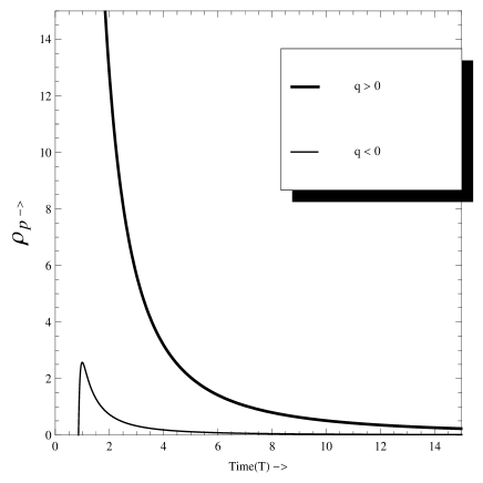
Figure 5 shows the comparative behaviour of particle energy density and string tension density versus time in the decelerating mode. It is observed that $\rho_{p}>\lambda$, i.e., particle energy density remains larger than the string tension density during the cosmic expansion (see, Refs. Kibble [31]; Krori et al. [99]), especially in early universe. This shows that massive strings dominate the early universe evolving with deceleration and in later phase will disappear which is in agreement with current astronomical observations.

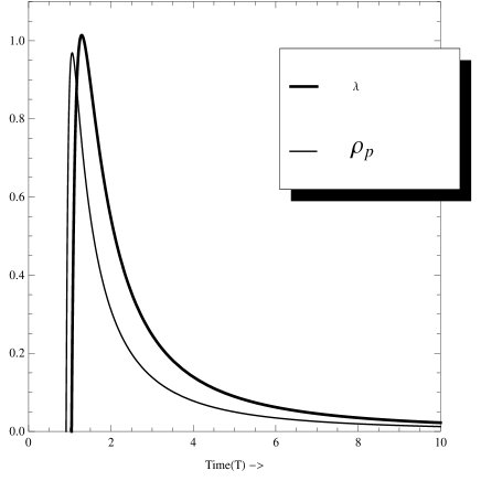
Figure 6 demonstrates the variation of $\rho_{p}$ and $\lambda$ versus the cosmic time for accelerating mode of the evolution. In this case, we observe that $\rho_{p}<\lambda$. Therefore, according to Kibble [31] and Krori et al. [99], strings dominate the universe evolving with acceleration. If this is so, we should have some signature of massive string at present epoch of the observations. However, it is not been seen so far.

It follows that the dynamics of the strings depends on the value of n or q. Further, it is observed that for sufficiently large times, the $\rho_{p}$ and $\lambda$ tend to zero. Therefore, the strings disappear from the universe at late time (i.e. present epoch). The same is predicted by the current observations.

The rate of expansion $H_{i}$ in the direction of x, y and z are given by

$$H_{x}=\frac{\dot{A}}{A}=\frac{3m\ell}{m+1}{T}^{-1}\;,$$ (37)

$$H_{y}=\frac{\dot{B}}{B}=\frac{3\ell}{2(m+1)}{T}^{-1}+\frac{1}{4}c_{4}(T)^{-\frac{3}{n}}\;,$$ (38)

$$H_{y}=\frac{\dot{B}}{B}=\frac{3\ell}{2(m+1)}{T}^{-1}-\frac{1}{4}c_{4}(T)^{-\frac{3}{n}}.$$ (39)

The Hubble parameter, expansion scalar and shear of the model are respectively given by

$$H=\ell(T)^{-1},$$ (40)

$$\theta=3\ell(T)^{-1},$$ (41)

$$\sigma^{2}=\frac{3\ell^{2}(2m-1)^{2}}{2(m+1)^{2}}{T}^{-2}+\frac{1}{4}c_{4}^{2}{T}^{-\frac{6}{n}}.$$ (42)

The spatial volume ($V$) and anisotropy parameter $(\bar{A})$ are found to be

$$V={T}^{\frac{3}{n}},$$ (43)

$$\bar{A}=\frac{1}{3}\sum_{i=1}^{3}{\left(\frac{\triangle H_{i}}{H}\right)^{2}}=\frac{(2m-1)^{2}}{(m+1)^{2}}+\frac{c_{4}^{2}}{6\ell^{2}}{T}^{\frac{2(n-3)}{n}},$$ (44)

where $\triangle H_{i}=H_{i}-H(i=1,2,3)$.

From the above results, it can be seen that the spatial volume is zero at $T=0$, and it increases with the cosmic time. The parameters $H_{i}$, H, $\theta$ and $\sigma$ diverge at the initial singularity. The mean anisotropic parameter is an increasing function of time for $n>3$ whereas for $n<3$ it decreases with time. Thus, the dynamics of the mean anisotropy parameter depends on the value of n. Since $\frac{\sigma^{2}}{\theta^{2}}=$ constant (from early to late time), the model does not approach isotropy through the whole evolution of the universe

3.2 String Cosmology with Exponential-law

Solving the equations (17), (22) and (24), we obtain the metric functions as

$$A(t)=c_{2}^{\frac{3m}{m+1}}\exp{\left(\frac{3m\ell}{m+1}t\right)}\;,$$ (45)

$$B(t)=\sqrt{c_{3}}c_{2}^{\frac{3}{2(m+1)}}\exp{\left[\frac{3\ell}{2(m+1)}t-\frac{c_{4}}{6\ell c_{2}^{3}}e^{-3\ell t}\right]},$$ (46)

$$C(t)=\frac{c_{2}^{\frac{3}{2(m+1)}}}{\sqrt{c_{3}}}\exp{\left[\frac{3\ell}{2(m+1)}t+\frac{c_{4}}{6\ell c_{2}^{3}}e^{-3\ell t}\right]}.$$ (47)

Figure 7: The plot of pressure $p$ versus $t$ in exponential-law expansion for $q=-1$.

Figure 8: The plot of energy density $\rho$ versus $t$ in exponential-law expansion for $q=-1$.

Figure 9: The plot of string tension density $\lambda$ versus $t$ in exponential-law expansion for $q=-1$.

Figure 10: The plot of particle density $\rho_{p}$ versus $t$ in exponential-law expansion for $q=-1$.

Therefore the metric (1) reduces to

$$ds^{2}=-dt^{2}+c_{2}^{\frac{6m}{m+1}}\exp{\left(\frac{6m\ell}{m+1}t\right)}(dx-zdy)^{2}+$$

$$c_{3}c_{2}^{\frac{3}{(m+1)}}\exp{\left[2\left\{\frac{3\ell}{2(m+1)}t-\frac{c_{4}}{6\ell c_{2}^{3}}e^{-3\ell t}\right\}\right]}dy^{2}$$

$$+\frac{c_{2}^{\frac{3}{(m+1)}}}{c_{3}}\exp{\left[2\left\{\frac{3\ell}{2(m+1)}t+\frac{c_{4}}{6\ell c_{2}^{3}}e^{-3\ell t}\right\}\right]}dz^{2}.$$ (48)

Eq. (16) gives either $\beta=0$ or $\frac{3}{2}\dot{\beta}+\frac{3}{2}\beta\left(\frac{\dot{A}}{A}+\frac{\dot{B}}{B}+\frac{\dot{C}}{C}\right)=0$. Therefore

$$\frac{\dot{\beta}}{\beta}=-\left(\frac{\dot{A}}{A}+\frac{\dot{B}}{B}+\frac{\dot{C}}{C}\right),$$ (49)

which reduces to

$$\frac{\dot{\beta}}{\beta}=-3\ell.$$ (50)

Integrating Eq. (50), we obtain

$$\beta=k_{1}e^{-3\ell t},$$ (51)

where $k_{1}$ is an integrating constant. From Eq. (51), it is observed that for $k_{1}>0$ and $\ell>0$, the displacement vector $\beta(T)$ is a decreasing function of time and it approaches to a small positive value at late time (i.e. present epoch), which is corroborated with Halford [4] as well as with the recent observations of SNe Ia. Recent cosmological observations of SNe Ia (Garnavich et al. [90, 91]; Perlmutter et al. [92]$-$[94]; Riess et al.[95, 96]; Schmidt et al. [97]).

The expressions for the isotropic pressure ($p$), the proper energy density ($\rho$), the string tension ($\lambda$) and the particle density ($\rho_{p}$) for the model (48) are obtained as

$$p=-\frac{9\ell^{2}(4m^{2}+2m+1)}{4(m+1)^{2}}-\frac{c_{4}^{2}}{4c_{2}^{6}}e^{-6\ell t}-\frac{1}{4}\exp{\left[-\frac{6\ell(1-m)}{m+1}t\right]}-\frac{3}{4}k^{2}_{1}e^{-6\ell t},$$ (52)

$$\rho=\frac{9\ell^{2}(4m+1)}{4(m+1)^{2}}-\frac{c_{4}^{2}}{4c_{2}^{6}}e^{-6\ell t}-\frac{1}{4}\exp{\left[-\frac{6\ell(1-m)}{m+1}t\right]}+\frac{3}{4}k^{2}_{1}e^{-6\ell t},$$ (53)

$$\lambda=\frac{9\ell^{2}(1-2m)}{2(m+1)}-\exp{\left[-\frac{6\ell(1-m)}{m+1}t\right]},$$ (54)

$$\rho_{p}=\frac{9\ell^{2}(4m^{2}+6m-1)}{4(m+1)^{2}}+\frac{3}{4}\exp{\left[\frac{6\ell(m-1)}{(m+1)}t\right]}-\frac{c_{4}^{2}}{4c_{2}^{6}}e^{-\ell t}+\frac{3}{4}k^{2}_{1}e^{-6\ell t}.$$ (55)

Figure 7 depicts the variation of pressure versus time for the exponential-law evolution of the universe. We observe that the pressure is negative and constant with the evolution of the universe. This is consistent with the well established fact that pressure is negative in the accelerating universe.

From Eq. (53), it is observed that the rest energy density $\rho$ is a constant function of time and $\rho>0$ always. The rest energy density has been graphed versus time in Figure 8. This means there is no density evolution in this set up. A possible reason for no evolution of density is that expansion of the Universe could be much rapid in which matter do not get time to re-adjust on expansion range or may be other unknown dominated effect which not incorporated in potential functions of this space-time for exponential-law.

From Eq. (54), it is observed that the tension density $\lambda$ is a decreasing function of time and $\lambda<0$ always. Figure 9 shows the plots of string tension density verses time However, initially it remains constant and then decreases more sharply with the cosmic time.

Figure 10 shows the plots of particle density versus time. In early stage of evolution, it increases with time and later stage it remains constant. From Eq. (55), it is evident that the particle density $\rho_{p}$ is an increasing function of time and $\rho_{p}>0$ for all time.

The expressions for kinematical parameters i.e. the scalar of expansion ($\theta$), shear scalar ($\sigma$), the spatial volume ($V$), average anisotropy parameter ($\bar{A}$) and deceleration parameter ($\rm q$) for the model (48) are given by

$$\theta=3\ell,$$ (56)

$$\sigma^{2}=\frac{3\ell^{2}(2m-1)^{2}}{4(m+1)^{2}}-\frac{c_{4}^{2}}{4c_{2}^{6}}e^{-6\ell t},$$ (57)

$$V=c_{2}^{3}e^{3\ell t},$$ (58)

$$\bar{A}=\frac{(2m-1)^{2}}{2(m+1)^{2}}-\frac{c_{4}^{2}}{6\ell^{2}c_{2}^{6}}e^{-6\ell t},$$ (59)

$$q=-1.$$ (60)

The rotation $\omega$ is identically zero. The negative value of $q$ indicates inflation. The evolution of the universe in such a scenario may not be consistent with the present day observations predicting an accelerated expansion.

The rate of expansion $H_{i}$ in the direction of x, y and z are given by

$$H_{x}=\frac{3m\ell}{m+1},$$ (61)

$$H_{y}=\frac{3\ell}{2(m+1)}+\frac{c_{4}}{2c_{2}^{3}}e^{-3\ell t},$$ (62)

$$H_{z}=\frac{3\ell}{2(m+1)}-\frac{c_{4}}{2c_{2}^{3}}e^{-3\ell t}.$$ (63)

Hence the average generalized Hubble’s parameter is given by

$$H=\ell.$$ (64)

From equations (61)-(63), we observe that the directional Hubble parameters are time dependent while the average Hubble parameter is constant.

It is observed that the physical and kinematic quantities are all constant at $t=0$ as well as $t\to\infty$. The expansion in the model is uniform throughout the time of evolution. We find that $\lim_{t\rightarrow 0}\frac{\sigma^{2}}{\theta^{2}}\neq 0$ and $\lim_{t\rightarrow\infty}\frac{\sigma^{2}}{\theta^{2}}\neq 0$, which show that this inflationary universe eventually does not approach isotropy for early as well as large values of $t$. The derived model is non-singular.

4 Conclusions

In this paper we have obtained a new class of spatially homogeneous and anisotropic Bianchi-II cosmological models in presence of perfect fluid distribution of matter representing massive strings within the framework of normal gauge in Lyra’s manifold by applying the variation law for generalized Hubble’s parameter that yields a constant value of deceleration parameter in general relativity. Secondly we have also assumed that the expansion in the model is proportional to the shear as Collins et al. [78] have showed that the normal congruence to the homogeneous expansion satisfies that the condition $\frac{\sigma}{\theta}=$ constant. The law of variation for Hubble’s parameter defined in (19) for B-II space-time models give two types of cosmologies, (i) first form (for $n\neq 0$) shows the solution for positive value of deceleration parameter for ($n>1$) and negative value of deceleration parameter for ($n<1$) indicating the power law expansion of the universe whereas (ii) second one (for $n=0$ shows the solution for negative value of deceleration parameter, which shows the exponential expansion of the universe. Exact solutions of Einstein’s field equations for these models of the universe have been obtained by using the two forms of average scale factor. The power law solutions represent the singular model where the spatial scale factors and volume scalar vanish at $T=0$. The energy density and pressure are infinite at this initial epoch. As $T\to\infty$, the scale factors diverge and $p$, $\rho$, $\lambda$ and $\rho_{p}$ tend to zero. $A_{m}$ and $\sigma^{2}$ are very large at initial time but decrease with cosmic time and vanish as $T\to\infty$. The exponential solutions represent singularity free model of the universe. In this case as $T\to-\infty$, the scale factors tend to zero which indicates that the universe is infinitely old and has exponential inflationary phase. All the parameters such as scale factor, $p$, $\rho$, $\lambda$, $\rho_{p}$, $\theta$, $\sigma^{2}$ and $A_{m}$ are constant at $t=0$.

Under the law of variation for Hubble’s parameter defined in (19), it has been shown that the two classes of solutions lead to the conclusion that, if $q>0$ the model expands but always decelerate whereas $q<0$ provides the exponential expansion and later accelerates the universe. The evolution of the universe in such a scenario is shown to be consistent with the present observations predicting an accelerated expansion.

The models presents the dynamics of strings in the accelerating and decelerating modes of evolution of the universe. It has been found that massive strings dominate in the decelerating universe whereas strings dominate in the accelerating universe. The strings dominate in the early universe and eventually disappear from the universe for sufficiently large times. This is in consistent with the current observations.

It is observed that the displacement vector $\beta(t)$ matches with the nature of the cosmological constant $\Lambda$ which has been supported by the work of several authors as discussed in the physical behaviour of the models in Subsections $3.1$ and $3.2$. In both cases (3.1) and (3.2) the the displacement vector $\beta$ is a decreasing function of time and it approaches to a small positive value at late time (i.e. present epoch), which is corroborated with Halford [4] as well as with the recent observations of SNe Ia (Garnavich et al. [90, 91]; Perlmutter et al. [92]$-$[94]; Riess et al. [95, 96]; Schmidt et al. [97]). In recent past there is an upsurge of interest in scalar fields in general relativity and alternative theories of gravitation in the context of inflationary cosmology [100, 101, 102]. Therefore the study of cosmological models in Lyra’s manifold may be relevant for inflationary models. There seems a good possibility of Lyra’s manifold to provide a theoretical foundation for relativistic gravitation, astrophysics and cosmology. However, the importance of Lyra’s manifold for astrophysical bodies is still an open question. In fact, it needs a fair trial for experiment.

It is remarkable to mention here that our work generalizes the results recently obtained by Kumar [103] in 2010. In absence of displacement field $\phi_{i}$ (i.e. by putting $k=0$ in case (3.1)), we obtain the results obtained by Kumar [103].

References

- [1] G Lyra Math. Z. 54 52 (1951)
- [2] D K Sen Z. Phys. 149 311 (1957)
- [3] D K Sen, K A Dunn J. Math. Phys. 12 578 (1971)
- [4] W D Halford Austr. J. Phys. 23 863 (1970)
- [5] W D Halford J. Math. Phys. 13 1699 (1972)
- [6] D K Sen, J R Vanstone J. Math. Phys. 13 990 (1972)
- [7] H H Soleng Gen. Rel. Gravit. 19 1213 (1987)
- [8] T Singh, G P Singh J. Math. Phys. 32 2456 (1991)
- [9] T Singh, G P Singh Il. Nuovo Cimento B 106 617 (1991)
- [10] T Singh, G. P. Singh Int. J. Theor. Phys. 31 1433 (1992)
- [11] T Singh, G P Singh Fortschr. Phys. 41 737 (1993)
- [12] G P Singh, K Desikan Pramana-Journal of Physics 49 205 (1997)
- [13] A Pradhan, A K Vishwakarma J. Geom. Phys. 49 332 (2004)
- [14] A Pradhan, V K Yadav, I Chakrabarty Int. J. Mod. Phys. D 10 339 (2000)
- [15] A Pradhan, L. Yadav, A K Yadav Astrophys. Space Sci. 299 31 (2005)
- [16] F Rahaman, S Chakraborty, M Kalam Int. J. Mod. Phys. D 10 735 (2001)
- [17] B B Bhowmik, A Rajput Pramana-Journal of Physics 62 1187 (2004)
- [18] J Matyjasek Int. J. Theor. Phys. 33 967 (1994) 967.
- [19] D R K Reddy Astrophys. Space Sci. 300 381 (2005)
- [20] R Casama, C A M de Melo, B M Pimentel Astrophys. Space Sci. 305 125 (2006)
- [21] F Rahaman, P Ghosh Fizika B 13 719 (2004)
- [22] F Rahaman, B Bhui, G Bag Astrophys. Space Sci. 295 507 (2005)
- [23] F Rahaman Int. J. Mod. Phys. D 9 775 (2000) 775
- [24] F Rahaman Int. J. Mod. Phys. D 10 579 (2001)
- [25] F Rahaman Astrophys. Space Sci. 281 595 (2002)
- [26] K Shanthi, V U M Rao Astrophys. Space Sci. 179 147 (1991)
- [27] R Venkateswarlu, D R K Reddy Astrophys. Space Sci. 182 97 (1991)
- [28] F Hoyle Mon. Not. Roy. Astron. Soc. 108 372 (1948)
- [29] F Hoyle, J V Narlikar Proc. Roy. Soc. London Ser. A 277 1 (1964)
- [30] F Hoyle, J V Narlikar Proc. Roy. Soc. London Ser. A 278 465 (1964)
- [31] T W B Kibble J. Phys. A: Math. Gen. 9 1387 (1976)
- [32] Ya B Zel’dovich, I Yu Kobzarev, L B Okun Sov. Phys.-JETP 40 1 (1975)
- [33] T W B Kibble Phys. Rep. 67 183 (1980)
- [34] A E Everett Phys. Rev. 24 858 (1981)
- [35] A Vilenkin Phys. Rev. D 24 2082 (1981)
- [36] Ya B Zel’dovich Mon. Not. R. Astron. Soc. 192 663 (1980)
- [37] P S Letelier Phys. Rev. D 20 1294 (1979)
- [38] P S Letelier Phys. Rev. D 28 2414 (1983)
- [39] J Stachel Phys. Rev. D 21 2171 (1980)
- [40] R Bali, S Dave Astrophys. Space Sci. 288 503 (2003)
- [41] R Bali, D K Singh Astrophys. Space Sci. 300 387 (2005)
- [42] R Bali, Anjali Astrophys. Space Sci. 302 201 (2006)
- [43] R Bali, U K Pareek, A Pradhan Chin. Phys. Lett. 24 2455 (2007)
- [44] R Bali, A Pradhan Chin. Phys. Lett. 24 585 (2007)
- [45] M K Yadav, A Pradhan, S K Singh, Astrophys. Space Sci. 311 423 (2007)
- [46] X X Wang Chin. Phys. Lett. 22 29 (2005)
- [47] X X Wang Chin. Phys. Lett. 23 1702 (2006)
- [48] B Saha, M Visinescu Astrophys. Space Sci. 315 99 (2008)
- [49] B Saha, V Rikhvitsky, M Visinescu arXiv:0812.1443 (2008)
- [50] M K Yadav, A Pradhan, A Rai Int. J. Theor. Phys. 46 2677 (2007)
- [51] D R K Reddy, Astrophys. Space Sci. 300 381 (2005)
- [52] D R K Reddy, D Rao, M V Rao Astrophys. Space Sci. 305 183 (2005)
- [53] V U M Rao, T Vinutha, K V S Sireesha Astrophys. Space Sci. 323 401 (2009)
- [54] V U M Rao, T Vinutha Astrophys. Space Sci. 325 59 (2010)
- [55] A Pradhan Fizika B 16 205 (2007)
- [56] A Pradhan Commun. Theor. Phys. 51 367 (2009)
- [57] A Pradhan, K Jotania, A Singh, Braz. J. Phys. 38 167 (2008)
- [58] A Pradhan, P Mathur Astrophys. Space Sci. 318 255 (2008)
- [59] A Pradhan, R Singh, J P Shahi Elect. J. Theor. Phys. 7 197 (2010)
- [60] S K Tripathi, D Behera, T R Routray Astrophys. Space Sci. 325 93 (2010)
- [61] A Pradhan, I Aotemshi, G P Singh Astrophys. Space Sci. 288 315 (2003)
- [62] A Pradhan, V Rai, S Otarod Fizika B 15 23 (2006)
- [63] A Pradhan, K K Rai, A K Yadav Braz. J. Phys. 37 1084 (2007)
- [64] A Pradhan, Jour. Math. Phy. 50 022501 (2009)
- [65] A Pradhan, S S Kumhar Astrophys. Space Sci. 321 137 (2009)
- [66] A Pradhan, P Mathur Fizika B 18 243 (2009)
- [67] A Pradhan, P Ram Int. Jour. Theor. Phys. 48 3188 (2009)
- [68] R Casama, C Melo, B Pimentel Astrophys. Space Sci. 305 125 (2006)
- [69] R Bali, N K Chandnani J. Math. Phys. 49 032502 (2008)
- [70] R Bali, N K Chandnani Fizika B 18 227 (2009)
- [71] S Kumar, C P Singh Int. Mod. Phys. A 23 813 (2008)
- [72] S. Ram, M Zeyauddin, C P Singh, Int. J. Mod. Phys. A 23 4991 (2008)
- [73] J K Singh Astrophys. Space Sci. 314 361 (2008)
- [74] V U M Rao, T Vinutha, M V Santhi Astrophys. Space Sci. 314 213 (2008)
- [75] K S Thorne Astrophys. J. 148 51 (1967)
- [76] R Kantowski, R K Sachs J. Math. Phys. 7 433 (1966)
- [77] J Kristian, R K Sachs, Astrophys. J. 143 379 (1966)
- [78] C B Collins, E N Glass, D A Wilkinson Gen. Rel. Grav. 12 805 (1980)
- [79] M S Berman Il Nuovo Cim. B 74 182 (1983)
- [80] M S Berman, F M Gomide Gen. Rel. Grav. 20 191 (1988)
- [81] B Saha, V Rikhvitsky Physica D 219 168 (2006)
- [82] B Saha Astrophys. Space Sci. 302 83 (2006)
- [83] C P Singh, S Kumar Int. J. Mod. Phys. D 15 419 (2006)
- [84] T Singh, R Chaubey Pramana - J. Phys. 67 415 (2006)
- [85] T Singh, R Chaubey Pramana - J. Phys. 68 721 (2007)
- [86] M Zeyauddin, S Ram Fizika B 18 87 (2009)
- [87] J P Singh, P S Baghel Int. J. Theor. Phys. 48 449 (2009)
- [88] A Pradhan, K Jotania Int. J. Theor. Phys. 49 1719 (2010)
- [89] R G Vishwakarma Class. Quant. Grav. 17 3833 (2000)
- [90] P M Garnavich Astrophys. J. 493 L53 (1998)
- [91] P M Garnavich Astrophys. J. 509 74 (1998)
- [92] S Perlmutter et al. Astrophys. J. 483 565 (1997)
- [93] S Perlmutter et al. Nature 391 51 (1998)
- [94] S Perlmutter et al. Astrophys. J. 517 565 (1999)
- [95] A G Reiss et al. Astron. J. 116 1009 (1998)
- [96] A G Reiss et al. Astron. J. 607 665 (2004)
- [97] B P Schmidt Astrophys. J. 507 46 (1998)
- [98] M A H MacCallum Comm. Math. Phys. 20 57 (1971)
- [99] K D Krori, T Chaudhuri, C R Mahanta, A Mazumdar Gen. Rel. Grav. 22 123 (1990)
- [100] G F R Ellis Standard and Inflationary Cosmologies (Preprint SISSA, Trieste 176/90/A) (1990)
- [101] D La, P J Steinhardt Phys. Rev. Lett. 62 376 (1989)
- [102] J D Barrow Phys. Lett. B 235 40 (1990)
- [103] S Kumar arXiv:010.0681 (2010)