A remark for dynamic equations on time scales

Abstract

We give a proposal to generalize the concept of the differential equations on time scales [1, 2, 3], such that they can be more appropriate for the analysis of real world problems, and give more opportunities to increase the theoretical depth of investigation.

url]http://www.metu.edu.tr/ marat

url]http://www.atilim.edu.tr/ mturan

1 Differential equations on time scales in Hilger’s sense and the first remark

Let us remind the differential equations on time scales, proposed by Hilger [1, 2, 3]. The main element of the equations is the time scale, which is understood as a nonempty closed subset, $\mathbb{T},$ of the real numbers. On a time scale ${\mathbb{T}},$ the functions $\sigma(t):=\inf\{s\in{\mathbb{T}}:s>t\}$ and $\rho(t):=\sup\{s\in{\mathbb{T}}:s<t\}$ are called the forward and backward jump operators, respectively. The point $t\in{\mathbb{T}}$ is called right-scattered if $\sigma(t)>t,$ and right-dense if $\sigma(t)=t.$ Similarly, it is called left-scattered if $\rho(t)<t,$ and left-dense if $\rho(t)=t.$

The $\Delta-$derivative of a continuous function $\varphi,$ at a right-scattered point is defined as

$$\varphi^{\Delta}(t):=\frac{\varphi(\sigma(t))-\varphi(t)}{\sigma(t)-t},$$ (1)

and at a right-dense point it is defined as

$$\varphi^{\Delta}(t):=\lim_{s\rightarrow t}\frac{\varphi(t)-\varphi(s)}{t-s},$$ (2)

if the limit exists.

A differential equation

$$y^{\Delta}(t)=f(t,y),\quad t\in{\mathbb{T}}$$ (3)

is said to be a differential equation on time scale, where function $f(t,y):{\mathbb{T}}\times{\mathbb{R}}^{n}\rightarrow{\mathbb{R}}^{n}$ in (3) is assumed to be rd-continuous on ${\mathbb{T}}\times{\mathbb{R}}^{n}$ [8].

If a point $t$ is right-dense, then the $\Delta$-derivative is the ordinary derivative. Otherwise, $t\in{\mathbb{T}}$ is a right-scattered point, and the $\Delta$-derivative is defined by means of the quotient. Let us discuss the second case more attentively. By the definition of the $\Delta-$derivative, assuming that $t$ is not an isolated point, one has that $\varphi(\sigma(t))=\varphi(t)+\varphi^{\prime}(t)(\sigma(t)-t).$ Now, compare this expression with the numerical approximation of the function on the interval $[t,\sigma(t)].$ Setting $\Delta t=\sigma(t)-t$ and $\Delta\varphi=\varphi(\sigma(t))-\varphi(t),$ we have that $\Delta\varphi=\varphi^{\prime}(t)\Delta t.$ Thus, one can see that the idea of the $\Delta-$derivative, as well as of the $\nabla-$derivative is close to the basic one for the numerical analysis [4]. See Figures 1 and 2 for illustration.

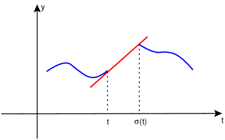
Figure 1:

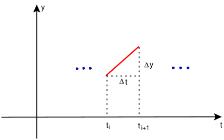
Figure 2:

That is, in its heart the concept of the differential equations on time scales is closely adjoint with numerical methods. However, for numerical methods, of course as far as the definition in $(\ref{dd1})$ is considered, smaller $\sigma(t)-t$ gives a better approximation. In the former theory of differential equations on time scales, the request was not considered, and the elements of linear change over the intervals near right-scattered (left-scattered) points are strong there. To return the non-linearity sense in the discussion, one needs to modify the equations. In our papers [5, 6, 7], the concept of transition conditions were proposed, when we consider the simple version of the time scale as a union of disjoint sections. In [5], these systems emerge as an auxiliary instrument of a discontinuous dynamical system investigation. In Section 3, we generalize this idea for all possible time scales.

2 Modeling proposals

In this part we shall answer two questions: Why the differential equations on time scales are needed by real world problems? How the Hilger’s equations can be extended for these? Consider a real world process, which can be symbolically given as a function $\psi(t),$ where $t$ is from a time scale. Suppose for this moment that the time scale admits only non-isolated moments. If the time is increasing, we have to prescribe what the value at $\sigma(t)$ is equal to for the right-scattered point $t.$ In Hilger’s theory, the value is evaluated by using the derivative of $\psi$ at the moment $t,$ and this is very restrictive, since the difference $\sigma(t)-t$ is not supposed to be small! It is reasonable to assume that there exists more general law of transition for $\psi$ from the moment $t$ to $\sigma(t).$ In general, it can be given with a function $\psi(\sigma(t))=J(t,\psi(t)).$ We call this expression as the transition condition. To illustrate, consider a population developing in time. We may assume that the size satisfies a local law in some borders, say in summer time, and it is not under the law in winter time. Moreover, the local law in winter time is not known. Nonetheless, we can evaluate the change in the time, that is the size at the beginning of the season and that at the end of the season. Assume that the change satisfies a new formula, which is naturally a discrete one. In that case, we come to the idea of the equations on time scales, but more general than those investigated before.

3 Differential equations on time-scales with transition conditions

Consider the time scale $\mathbb{T}$ given above, and the same $\Delta-$derivative of a continuous function $\varphi,$ defined by (1) and (2).

Denote by ${\mathbb{T}}_{\sigma}$ the set of all right-scattered points of ${\mathbb{T}}.$ Consider a function $f(t,y):{\mathbb{T}}\backslash{\mathbb{T}}_{\sigma}\times{\mathbb{R}}^{n}\rightarrow{\mathbb{R}}^{n},$ which is assumed to be rd-continuous on ${\mathbb{T}}\backslash{\mathbb{T}}_{\sigma}\times{\mathbb{R}}^{n}.$ Define a function $J(t,y):{\mathbb{T}}_{\sigma}\times{\mathbb{R}}^{n}\rightarrow{\mathbb{R}}^{n}.$ Now, on the time scale, we introduce a piecewise function $F(t,y),$ which is equal to the function $f(t,y),$ if $t$ is a right-dense point, and it is equal to $J(t,y),$ if $t$ is a right-scattered point. We suggest to consider the following differential equation on the time scale

$$y^{\Delta}(t)=F(t,y),\quad t\in{\mathbb{T}}.$$ (4)

Condition that all solutions are continuous on the time scale should be assumed.

To demonstrate the opportunities, which one can have with the newly introduced equations, consider the following theorem of existence and uniqueness.

Theorem 3.1

Let ${\mathbb{T}}$ be a time scale, $t_{0}\in{\mathbb{T}},$ $y_{0}\in{\mathbb{R}}^{n},$ $a>0$ with $\inf{\mathbb{T}}\leq t_{0}-a$ and $\sup{\mathbb{T}}\geq t_{0}+a,$ and put

$$I_{a}=(t_{0}-a,t_{0}+a)\quad and\quad U_{b}=\{y\in{\mathbb{R}}^{n}:|y-y_{0}|<b\}.$$

Suppose that $f:I_{a}\times U_{b}\to{\mathbb{R}}^{n}$ is rd-continuous, bounded with bound $M>0,$ Lipschitz continuous with Lipschitz constant $L>0,$ and

$$\left\|\frac{J(t,y)}{\sigma(t)-t}\right\|\leq N$$

for all $t\in{\mathbb{T}}_{\sigma}\cap I_{a}$ and $y\in U_{b}.$ Then the IVP

$$y^{\Delta}=F(t,y),\quad y(t_{0})=y_{0},$$ (5)

has exactly one solution on $[t_{0}-\alpha,t_{0}+\alpha],$ where

$$\alpha=\min\left\{a,\frac{b}{\max\{M,N\}},\frac{1-\varepsilon}{L}\right\}\quad for\ some\ \varepsilon>0.$$

If $t_{0}\in{\mathbb{T}}_{\sigma}$ and $\alpha<\sigma(t_{0})-t_{0},$ then the unique solution exists on the interval $[t_{0}-\alpha,\sigma(t_{0})].$

One could compare the last assertion with the following, from [8]. The condition on the transition function $J$ is added, in this particular case. In general, properties of the function will generate new theoretical, and what is most important, application prospects for these equations. One can see that many results in the theory, which have been obtained earlier can, now, be generalized, for newly proposed systems with additional interesting properties that transition conditions can admit.

Another opportunity is to consider state-dependent time scales [7]. Let a set $\mathcal{D}$ in $\mathbb{R}\times\mathbb{R}^{n},$ be given, such that for each $x\in{\mathbb{R}}^{n},$ the projection of the intersection, ${\cal D}_{x},$ of the line $(t,x),t\in\mathbb{R}$ with $\cal D$ on the time axis is a time scale in the sense of Hilger. Thus, one can define the function $\sigma(t,x)=\sup\{s\in{\mathcal{D}}_{x}:s>t\}$ for each point $(t,x)\in{\cal D}.$ We assume that the function $\sigma$ is continuous in $x.$ If the moment $t$ is such that $(t,\varphi(t))$ is right-dense in the correspond time scale, ${\cal D}_{\varphi(t)},$ then the $\Delta-$derivative is defined by (2). Otherwise it is equal to

$$\varphi^{\Delta}(t):=\frac{\varphi(\sigma(t,\varphi(t)))-\varphi(t)}{\sigma(t,\varphi(t))-t}.$$ (6)

Now, define a function $G(t,x),$ which is equal to a continuous function $f(t,x)$ at a right-dense point $(t,x),$ and to function $J(t,x),$ if the point is a right-scattered one. Then, one can discuss the following equation

$$y^{\Delta}(t)=G(t,y),\quad(t,y)\in{\cal D}.$$ (7)

It is obvious that the equations with state-dependent time scales can also play a certain role in this theory, and they will be used in the modeling of real world problems. The analysis may be of great interest, since new opportunities related to the non-linear properties of the time scales will emerge.

4 Unification of differential equations with discontinuities

Finally, we want to mention that very profitable ways for differential equations on time scales is to investigate them together with different types of discontinuities. These days there are several well extended theories such that systems with discontinuities in the right-hand-side, arguments, impulsive differential equations. They are realized in very interesting application projects as well [9]-[18]. We are sure that integration of the methods and results of these theories with above mentioned extensions of differential equations on time scales can provide really interesting horizons, which can give a light on new ways for modeling processes in mechanics, electronics, medicine, biology. One of the particular results in this sense is our recent paper [6], where certain class of differential equations on time scales is embedded in differential equations with fixed moments of impulses.

References

- [1] S. Hilger, Ein Maßkettenkalkül mit Anvendung auf Zentrums , PhD thesis, Universität Würzburg, 1988.
- [2] B. Aulbach and S. Hilger, A unified approach to continuous and discrete dynamics, 53, Qualitative theory of Differential Equations, Szeged, Hungary, 1988.
- [3] S. Hilger, Analysis on measure chains - a unified approach to continuous and discrete calculus, Results Math. 18 (1990) 18-56.
- [4] J. Stoer, R. Bulirsch, Introduction to numerical analysis, Springer-Verlag, New York (1980).
- [5] M. U. Akhmet, Perturbations and Hopf bifurcation of the planar discontinuous dynamical system, Nonlinear Analysis, 60 (2005) 163 - 178.
- [6] M. U. Akhmet, M. Turan, The differential equations on time scales through impulsive differential equations, Nonlinear Analysis, 65 (2006) 2043 - 2060.
- [7] M. U. Akhmet, M. Turan, Differential equations on variable time scales, Nonlinear Analysis: Theory, Methods and Applications 70 (2009) 1175 - 1192.
- [8] M. Bohner, A. Peterson, Dynamic equations on time scales: an introduction with applications, Birkhäuser (2001).
- [9] J. Awrejcewicz, C. H. Lamarque, Bifurcation and chaos in nonsmooth mechanical systems, World Scientific, Singapore, 2003.
- [10] M. di Bernardo, C. J. Budd, A.R. Champneys and P. Kowalczyk, Piecewise-smooth dynamical systems, Springer-Verlag, London, 2008.
- [11] B. Brogliato, Nonsmooth impact mechanics, Springer-Verlag, London, 1996.
- [12] L. Dai,Nonlinear dynamics of piecewise constant systems and implementation of piecewise constant arguments, World Scientific, Hackensack, NJ, 2008.
- [13] A. F. Filippov, Differential equations with discontinuous right hand sides, Kluwer, Dordrecht, 1988.
- [14] F. C. Hoppensteadt, C. S. Peskin, Mathematics in Medicine and in the Life Sciences, Springer-Verlag, New York, Berlin, Heidelberg, 1992.
- [15] A. Katok, J.-M. Strelcyn, F. Ledrappier and F. Przytycki, Invariant manifolds, entropy and billiards; smooth maps with singularities, Lecture Notes in Mathematics, 1222, Springer-Verlag, Berlin, 1986.
- [16] V.Lakshmikantham, X. Liu,Impulsive hybrid systems and stability theory, Dynam. Systems Appl., 7, no. 1, (1998) 1-9.
- [17] A. M. Samoilenko, N. A. Perestyuk, Impulsive Differential Equations, World Scientific, Singapore, 1995.
- [18] J. Wiener, Generalized Solutions of Functional Differential Equations, World Scientific, Singapore, 1993.