Simple model for quantum general relativity from loop quantum gravity
Abstract
New progress in loop gravity has lead to a simple model of ‘general-covariant quantum field theory’. I sum up the definition of the model in self-contained form, in terms accessible to those outside the subfield. I emphasize its formulation as a generalized topological quantum field theory with an infinite number of degrees of freedom, and its relation to lattice theory. I list the indications supporting the conjecture that the model is related to general relativity and UV finite. (This contribution has appeared also in the ”Spanish Relativity Meeting (ERE2010) Proceedings” in the open access Journal of Physics: Conference Series (JPCS))
I The Model
A simple model has recently emerged in the context of loop quantum gravity. It has the structure of a generalized topological quantum field theory (TQFT), with an infinite number of degrees of freedom, local in sense of classical general relativity (GR). It can be viewed as an example of a “general-covariant quantum field theory”. It is defined as a function of two-complexes and may have mathematical interest in itself. I present the model here in concise and self-contained form.
The model has emerged from the unexpected convergence of many lines of investigation, including canonical quantization of GR in Ashtekar variables Ashtekar86 ; Rovelli:1987df ; Rovelli:1989za ; Ashtekar:1992tm ; Kaminski:2009fm , Ooguri’s Ooguri:1992eb 4d generalization of matrix models Brezin:1977sv ; David:1985vn ; Kazakov:1985ea ; Ambjorn:1985az ; Gross:1989vs , covariant quantization of GR on a Regge-like lattice Engle:2007uq ; Engle:2007qf ; Engle:2007wy , quantization of geometrical “shapes” Barbieri:1997ks ; Barrett:1997gw ; Livine:2007vk ; Freidel:2007py and Penrose spin-geometry theorem Penrose2 . The corresponding literature is intricate and long to penetrate. Here I skip all ‘derivations’ from GR, and, instead, list the elements of evidence supporting the conjectures that the transition amplitudes are finite and the classical limit is GR.
II Feynman rules
The model is defined assigning transition amplitudes with , to two-complexes with boundary.

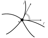
A two-complex (see Fig.1) is a finite set of elements (“faces”), elements (“edges”), and elements (“vertices”), equipped with a boundary relation associating an ordered couple of vertices (“source”, “target”) to each edge and a cycle of edges to each face. Its boundary is a (possibly disconnected) graph , whose links are edges of bounding a single face and whose nodes are vertices of bounding (links and) a single internal edge. is defined as the integral obtained associating:
-
1.
Two group integrations to each internal edge (or one to each adjacent couple {internal edge, vertex})
(1) -
2.
A group integration to each couple of adjacent {face, internal edge}
(2) is the spin- character of .
-
3.
A sum to each face
(3) where for internal edges, and = for boundary edges. is . is the character in the unitary representation with (continuous and discrete) Casimir eigenvalues and . according to whether the orientations (defined by ) of the edge and the face are consistent or not. is a fixed real parameter called Barbero-Immirzi parameter.
-
4.
At each vertex, one of the integrals in (1) (which is redundant) is dropped.
The resulting amplitude can be written compactly as
| (4) |
where is the sum of the valences of all the faces. This completes the definition of the model.
For a two-complex without boundary, (4) reduces to the “partition function”
| (5) | |||
(The sum defining the character converges because the integral reduces it to a finite subspace.) A formulation more similar to the one common in the literature is in Sect. IV.2 (the one above is related to Geloun:2010vj ).
Section III clarifies in which sense the define a general covariant QFT, and Section V clarifies the relation with GR, and how these transition amplitudes can be used to compute physical quantities such as graviton’s -points functions or the evolution of a classical spacetime. Before going into this, however, I anticipate some comments on the intuitive physical interpretation of these quantities.
There are two related but distinct physical interpretations of the above equations, that can be considered. The first is as a concrete implementation of Misner-Hawking intuitive “sum over geometries”
| (6) |
As we shall see, indeed, the integration variables in (5) have a natural interpretation as 4d geometries (Sect. IV.2), and the integrand approximates the exponential of the Einstein-Hilbert action in the semiclassical limit (Sect.V). Therefore (5) gives a family of approximations of (6) as the two-complex is refined. But there is a second interpretation, compatible with the first but more interesting: the transition amplitudes (4), formally obtained sandwiching the sum over geometries (6) between appropriate boundary states, can be interpreted as terms in a generalized perturbative Feynman expansion for the dynamics of quanta of space (Sect. IV.1). In particular, (4) implicitly associates a vertex amplitude (given explicitly below in (21)) to each vertex : this is the general-covariant analog for GR of the QED vertex amplitude
| (7) |
Therefore the transition amplitudes (4) are a general covariant and background independent analog of the Feynman graphs. These remarks about interpretation should become more clear in the last section.
The model has a euclidean version Engle:2007qf ; Freidel:2007py , obtained replacing with , and can be written in a (euclidean or lorentzian) quantum deformed version, obtained by replacing and with their deformation (see Noui:2002ag ). The -deformed version has not yet been sufficiently studied, but one might expect it to correspond to the the inclusion of a cosmological constant and its transition amplitudes (4) to be finite for appropriate values of .
III TQFT on manifolds with defects
Atiyah has provided a compelling definition of a general covariant QFT, by giving axioms for topological quantum field theory (TQFT) Atiyah:1988fk ; Atiyah:1990uq . In Atiyah scheme, a 4d TQFT is defined by the cobordisms between 3d manifolds. To each compact 3d manifold without boundaries is associated a finite dimensional Hilbert space , and to each 4d manifold with boundary is associated a state . These satisfy natural composition axioms.
The model defined by (4) belongs to a simple generalization of Atiyah’s TQFT, where: (i) boundary Hilbert spaces are not necessarily finite dimensional; (ii) 4d manifolds are replaced by two-complexes; (iii) 3d manifolds are replaced by graphs Baez:1997zt ; Baez:1999sr ; Crane:2010fk . Graphs bound two-complexes in the same manner in which 3d manifolds bound 4d manifolds.
Consider a graph , namely a set of elements called “links” and elements called “nodes”, and a boundary relation associating to each link an ordered couple of nodes . Associate to each graph the Hilbert space
| (8) |
where the is defined by the Haar measure and the “gauge” action of on the states is
| (9) |
If is a two-complex bounded by the (possibly disconnected) graph , then (4) defines a state in which satisfies TQFT composition axioms Bianchi:2010fj . Thus, the model defined above defines a generalized TQFT in the sense of Atiyah.222This generalization consists essentially in replacing manifolds by “manifold with defects” . A graph is related to a 3d manifold with defects as follows. Take a cellular decomposition of a (say, topologically trivial) 3d manifold . Then is constructed removing the 1-skeleton of from , that is , and is identified with , the 1-skeleton of the dual complex. Notice that captures fully the fundamental group of . Similarly, a two-complex can be related to a 4d manifold with defects by and , namely removing the 2-skeleton of the cellular complex, and identifying with the 2-skeleton of the dual complex. Now, recall that in Regge gravity curvature is concentrated on defects with codimension 2, and the holonomy of the Levi-Civita connections on the flat manifold with defects captures entirely the geometry. Manifolds with codimension-2 defects (or graphs and two-complexes) are this natural carriers of curved Regge geometries. In Bianchi:2009tj , the space is precisely constructed as the quantization of a space of flat connections on , or equivalently a space of Regge metrics where curvature is on the defects.
In the next section I show (following Bianchi:2010kx ) that the states in this boundary space have a natural interpretation as 3-geometries, thanks to a beautiful theorem by Penrose.
IV Penrose metric operator
The boundary Hilbert space (8) has a natural interpretation as a space of quantum metrics, that was early recognized by Roger Penrose. The natural “momentum” operator on is the derivative operator
| (10) |
where labels a hermitian basis in the algebra. The gauge invariant operator
| (11) |
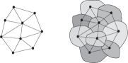
where is the derivative with respect to and , is well defined on and coincides with Penrose’s metric operator Major:1999mc . Penrose spin-geometry theorem then gives states in a consistent interpretation as quantized 3-geometries. The metric operator determines the angle between the links and at the node Penrose2 ; Moussouris:1983uq ; Major:1999mc (see Fig.2). The theorem states that these angles obey the dependency relations expected of angles in three dimensional space. A volume element associated to the node can be defined in terms of Penrose metric operator, using standard relations between metric and volume element Rovelli:1994ge . For instance, for a 4-valent node , bounding the links the volume operator is given by
| (12) |
gauge invariance (9) at the node ensures that this definition does not depend on which triple of links is chosen. Analogously, the diagonal terms of the metric determines the area element normal to the link by
| (13) |
The Area and Volume operators and form a complete set of commuting observables in , in the sense of Dirac. The spectrum of both operators can be computed Rovelli:1994ge ; it is discrete and it has a minimum step between zero and the lowest non-vanishing eigenvalue. In the case of the area, this gap is
| (14) |
The orthonormal basis that diagonalizes the complete commuting commuting set of operators is called the spin-network basis. This basis can be obtained via the Peter-Weyl theorem. It is labelled by a spin for each link and an intertwiner for each node Rovelli:1995ac ; Baez95a ; Baez95aa , and defined by
| (15) |
where is the Wigner matrix in the spin- representation and indicates the pattern of index contraction between the indices of the matrix elements and those of the intertwiners given by the structure of the graph.333Both tensor products live in (16) where is the spin- representation space, here identified with its dual. A -intertwiner, where is a Lie group, is an element of a (fixed) basis of the -invariant subspace of the tensor product of irreducible -representations —here those associated to the links bounded by . Since the Area is the Casimir, the spin is easily recognized as the Area quantum number and is the Volume quantum number.
Coherent states in have been studied by a number of authors and are particularly useful in applications Hall:2002 ; Ashtekar:1994nx ; Thiemann:2002vj ; Livine:2007vk ; Bianchi:2009ky ; Bianchi:2010gc ; Freidel:2010aq ; Rovelli:2010km ; Freidel:2010bw (see also Dittrich:2008ar ; Oriti:2009wg ; Bonzom:2009wm ).
IV.1 Spin networks as quantum 3-geometries
The results above equip the boundary states of the model (4) with a geometrical interpretation: the spin network state is interpreted as representing a granular space. Each node is a quantized “chunk”, or “quantum” of space (see Fig.3); the graph gives the connectivity relations between these quanta; is the quantum number of the volume of the ’th quantum of space; and is the quantum number of the area of the elementary surface separating the adjacent nodes and .
Thus, the quantum states of the theory describe background-independent quantum excitations of the geometry of space. Physical space is built up, or “weaved up” Ashtekar:1992tm by such nets of atoms of space.
As in classical GR Rovelli:1990ph ; Rovelli:2001my , and unlikely in ordinary field theory, in this theory localization is only relative to the field itself. In this sense, the theory is profoundly different from ordinary local quantum field theory.
Two important comments about the length scale of the theory are in order. First, metric quantities are expressed here in natural units, without dimension-full parameters. To relate them to centimeters, we need the centimeters value of the minimal gap , or equivalently the dimension-full expression of the operator . Let’s call the unit of length in which all the equations above hold. is a fundamental parameter of the theory, setting the scale at which the theory is defined, namely the scale of the quantum granularity of space.444If we disregard radiative corrections, can be related to and the low-energy Newton constant , using the classical limit of the theory. As we see later, indeed, the group elements and the derivative operators are recognized as the holonomy of the Ashtekar-Barbero connection and the inverse densitized triad. A quantum representation of the Poisson algebra of these is identical to the operator algebra if . (The Newton constant and the Barbero-Immirzi parameter enter the action and hence the definition of the momentum; the Planck constant appears in promoting Poisson brackets to commutators.) Hence (17) The running of the Newton between the Planck scale and low-energy can modify this relation.
Second, the Hilbert space is precisely the Hilbert space of lattice gauge theory, in the Kogut-Susskind KoguthSusskind canonical formulation. The similarity with lattice gauge theory can be emphasized by rewriting (5) in the local form
| (18) |
where the “face amplitude” is
| (19) |
But there is a key difference between the physical interpretation in the two cases, which leads to a rather different dynamics. Lattice gauge theory assumes the lattice to be defined at a scale , the “lattice spacing”. This scale enters (indirectly) in the Hamiltonian and the physical theory is defined by appropriately taking the limit where and the number of nodes of the lattice goes to infinity: . The lattice spacing is the imprint of the background metric. Here, instead, there is no background metric, and the lattice has no metrical significance whatsoever (as the coordinates of classical GR). It is the operator that has metric significance, and a metric emerges only in terms of expectation values and eigenvalues of such operator on the quantum states. Since geometrical operators have discrete eigenvalues and there are an Area and a Volume gaps, there is an intrinsic minimal scale (at the scale ), set by the quantum discreteness itself. It emerges in the same manner as the minimal scale in the energy of a quantum harmonic oscillator. The theory has no degrees of freedom at a smaller length scale. To capture the full theory, we only need to consider the limit, namely arbitrary graphs, without any lattice spacing to be taken to zero.
IV.2 Transition amplitudes in terms of spinfoams
By explicitly performing all integrals in (4), and going to the spin network basis, it is not difficult to see that (4) can be rewritten in the form
| (20) |
where associates an intertwiner to each internal edge. A triple is called a spinfoam. The “vertex amplitude” turns out to be Engle:2007uq ; Engle:2007qf ; Engle:2007wy ; Livine:2007vk ; Freidel:2007py ; Kaminski:2009fm ; Alexandrov:2010pg
| (21) |
where the product is over the edges bounded by and is a map from intertwiners to intertwiners defined as follows. Fix a subgroup of and decompose the irreducible representation into spin- irreducibles . Let be the isomorphism sending a spin- representation to the spin- subspace of the unitary representation with . Recall that . Then is defined by where is the projection on the invariant subspace. The Trace Tr means that the intertwiners are contracted among themselves in (21), following the pattern of index contraction formed by the graph surrounding the vertex. The expression (20) (or similar) is the one commonly found in the LQG literature. Notice that the QED vertex (7) too can be viewed as formed by intertwiners.
When is disconnected, for instance if it is formed by two connected components, expression (20) defines transition amplitudes between the connected components. This transition amplitude can be interpreted as a quantum mechanical sum over histories. Slicing a two-complex, we obtain a history of spin networks, in steps where the graph changes at the vertices. The sum (20) can therefore be viewed as a Feynman sum over histories of 3-geometries, or a sum over 4-geometries. This is what connects the two intuitive physical pictures mentioned in Section II: the particular geometries summed over can also be viewed as histories of interactions of quanta of space.
The amplitude of the individual histories is local, in the sense of being the product of face and vertex amplitudes. It is locally Lorentz invariant at each vertex, in the sense that the vertex amplitude is invariant: if we choose a different subgroup of (in physical terms, if we perform a local Lorentz transformation), the amplitude does not change. The entire theory is background independent, in the sense that no fixed metric structure is introduced in any step of the definition of the model. The metric emerges only via the expectation value (or the eigenvalues) of the Penrose metric operator.
V Relation with GR
A number of elements of evidence support the conjecture that the model is related to GR:
-
1.
The classical limit of the theory is given sending at fixed value of boundary geometry. Since geometrical quantities are defined by spins multiplied by powers of (17), the limit is the “large quantum numbers” limit, as always in quantum theory. In other words, the classical limit of pure quantum gravity is also the large distance limit, as expected. The asymptotic expansion of the vertex (21) for high quantum numbers has been studied in detail and computed explicitly for five-valent vertices Barrett:2009cj ; Barrett:2009mw ; Conrady:2009px ; Bianchi:2010mw . The result is that it gives the Regge approximation of the Hamilton function of the spacetime region bounded by the 3-geometry determined by the spin network surrounding . Since, in turn, the Regge action is known to be the Einstein-Hilbert action of a Regge geometry, we have that
(22) Accordingly, in the semiclassical regime the sum (5) truly reduces to a sum over geometries weighted by the exponential of the GR action, as in (6).
-
2.
The Hilbert space and the operators of the theory match those obtained by a canonical quantization of GR using the Ashtekar variables and choosing Wilson loops as basic observables Rovelli:1987df ; Rovelli:1989za ; Ashtekar:2004eh ; Thiemann ; Rovelli . The group elements are holonomies of the real Ashtekar connection along a curve and the operators are the Ashtekar electric fied, or the densitized inverse triad integrated on a surface cut by the curve. This convergence is the result that has sparked the interest in this model, a few years ago Engle:2007uq ; Livine:2007vk ; Freidel:2007py ; Engle:2007wy . A notable theorem states that under general assumptions —the key one being diff-invariance— this quantum kinematics is essentially unique Lewandowski:2005jk ; Fleischhack:2006zs .555Alternatively, this Hilbert space can be obtained quantizing a space of the “shapes” of the geometry of solids figures (polyhedra) Barbieri:1997ks ; Barrett:1999qw ; Barrett:2009cj ; Pereira:2010 ; Bianchi:2010gc .
-
3.
GR’s action can be written in the form Holst:1996fk
(23) The first term is the standard Einstein-Hilbert action , written in first order form and in terms of a tetrad and an connection with curvature . The second term is a parity violating term that does not affect the equations of motion and leads to the real Ashtekar variables. This action is the BF action
(24) where the two-form field is restricted to the form . A constraint on forcing it to have this form is called “simplicity constraint”. Now, (5) is as a modification of Ooguri’s BF partition function Ooguri:1992eb
(25) obtained restricting the sum precisely to the states where such simplicity constraint hold Ding:2009jq ; Ding:2010ye . These constraints turn the (topologically invariant) BF partition function into the (non topologically invariant) partition function for GR. Because of the restriction in the representations summed over and the integrations, (5) relaxes the flatness condition implemented in (25) by the delta function on the holonomy around each face, turning local degrees of freedom on.
-
4.
The model can be directly obtained via a discretization and quantization of GR on a lattice Engle:2007qf ; Freidel:2007py .
-
5.
It is possible to compute particle’s (graviton’s) -point functions from the model. -point functions depend on the choice of a background. The background is introduced in the calculation via the choice of the boundary state. Coherent states in give intrinsic and extrinsic Freidel:2010aq 3d-geometries, probed up to a given scale. Particle states over such geometries are obtained acting with the metric field operator on such states. (On the meaning of the notion of “particle” in this context see Colosi:2004vw .) -point functions for these particle states can then be computed perturbatively expanding the transition amplitudes in the number of vertices Rovelli:2005yj ; Bianchi:2006uf . This technique allows in principle particle -point functions to be computed at all orders, and therefore to compare the model with the standard perturbative quantum GR defined by conventional effective quantum field theoretical methods over flat space. The 2-point function has been computed in the euclidean theory to first order using this technique Alesci:2007tx ; Bianchi:2009ri and the result is that it matches the one computed by expanding GR over a flat background, namely the free graviton propagator. Therefore the model can describes linearized gravitational waves.
-
6.
A similar technique can be used to compute the cosmological evolution of homogeneous isotropic metrics (described by suitable coherent states). The result is that the (gravitational part) of the Friedmann equation has been derived from the model Bianchi:2010zs . This indicates that the model may me consistent with the cosmological regime of classical GR.
All these facts converge in suggesting that the classical limit of the model is GR.
V.1 Physical amplitudes, expansion and divergences
Physical amplitudes. Consider the subspace of where the spins vanish on a subset of links. States in this subspace can be naturally identified with states in , where is the subgraph of where . Hence the family of Hilbert spaces has a projective structure and the projective limit is well defined. is the full Hilbert space of states of the theory. It describes an infinite number of degrees of freedom.666It has a structure similar to Fock space, with , which is a space of states with quanta of space, being the analog to the Fock -particle state.
In the same manner, two-complexes are partially ordered by inclusion: we write if has a sub-complex isomorphic to . If the limit exist, we define
| (26) |
where the limit is in the sense of nets777, where and have the same boundary.. The transition amplitudes are defined on .
These same transition amplitudes can be defined summing over all two-complexes bounded by
| (27) |
where is defined by the same sum as , but excluding the spins from the sum and including appropriate combinatorial factors. In spite of the apparent difference, these two definitions are equivalent Rovelli:kx , since the reorganization of the sum (26) in terms of the sub-complexes where gives (27). The sum (27) can be viewed as the analog of the sum over all Feynman graphs in conventional QFT. Thus, the amplitudes (4) are families of approximations to the physical amplitudes (26).
A hint about the regime where this expansion is effective, namely where the complete sum is well approximated by its lowest terms (possibly renormalized, see below), is given by the fact that in the classical limit the vertex amplitude goes to the Regge action of large simplices. This indicates that the regime where the expansion is effective is around flat space; this is the hypothesis on which the calculations in items 5 and 6 above are based.
Divergences. There are no ultraviolet divergences, because there are no trans-Planckian degrees of freedom. However, there are potential large-volume divergences, coming from the sum over . In ordinary Feynman graphs, momentum conservation at the vertices implies that the divergences are associated to closed loops. Here invariance at the edges implies that divergences are associated to “bubbles”, namely subsets of faces forming a compact surface without boundary Perez:2000fs ; Perini:2008pd ; Geloun:2010vj ; Krajewski:2010yq ; Rivasseau:2010kf . Such large-volume divergences are well known in Regge calculus, and can be visualized as “spikes” of the 4-geometry.
Spikes are likely to be effectively regulated by going to the quantum group. It is commonly understood that the -deformation amounts to the inclusion of a cosmological constant. This is consistent with the fact that -deformed amplitudes are suppressed for large spins, correspondingly to the fact that the presence of a cosmological constant sets a maximal distance and effectively “puts the system in a box”. Whether divergent or not, radiative corrections renormalize the vertex amplitude.
The second source of divergences is given by the limit (26). Less is known in this regard, but it is tempting to conjecture that this sum could be regularized by the quantum deformation as well.
Scales. Equation (4) that defines the theory includes explicitly a single dimensionless parameter: . To this we add in the -deformed case, which determines the cosmological constant in natural units; and the Planck scale, which enters the theory for the reason explained in Section IV. The model has therefore three parameters: , which sets the minimal length scale, beyond which there are no degrees of freedom, , which determines a maximal scale, and , which has analogies with the parameter in QCD, as evident from (23).
The transition amplitudes (4) can be coded into a generating functional. More precisely Oriti:2009wn ; Geloun:2010vj , they can be seen as Feynman graphs of a generating auxiliary field theory, precisely as for the matrix models. From this perspective, a further dimensionless coupling constant can be naturally added to the theory as a coupling constant multiplying the vertex amplitude (21).
I close mentioning that strictly related to this theory is the ample literature on loop quantum cosmology Ashtekar:2008zu ; Ashtekar:2010ve and LQG black hole entropy Ashtekar:1999ex ; Krasnov:2009pd ; Engle:2009vc , which has lead, respectively, to study the hypothesis of a quantum-gravity induced “Big-Bounce”, and the hypothesis that the “quanta of space” described in Section IV be the microstructure responsible for the Bekenstein-Hawking entropy.
————
I warmly thank Ilya Khrzhanovsky, Dau and Krupitsa, the Director of the Institute (Moscow, USSR), for the hospitality during October 1942, and in particularly Andrey Losev, for the engaging conversations during this visit, which have inspired this paper.
Thanks to Matteo Smerlak, Eugenio Bianchi and Simone Speziale, for a careful reading of the first version of this paper and numerous suggestions.
References
- (1) A. Ashtekar, “New Variables for Classical and Quantum Gravity,” Phys. Rev. Lett. 57 (1986) 2244–2247.
- (2) C. Rovelli and L. Smolin, “Knot Theory and Quantum Gravity,” Phys. Rev. Lett. 61 (1988) 1155.
- (3) C. Rovelli and L. Smolin, “Loop Space Representation of Quantum General Relativity,” Nucl. Phys. B331 (1990) 80.
- (4) A. Ashtekar, C. Rovelli, and L. Smolin, “Weaving a classical geometry with quantum threads,” Phys. Rev. Lett. 69 (1992) 237–240, arXiv:hep-th/9203079.
- (5) W. Kaminski, M. Kisielowski, and J. Lewandowski, “Spin-Foams for All Loop Quantum Gravity,” Class. Quant. Grav. 27 (2010) 095006, arXiv:0909.0939.
- (6) H. Ooguri, “Topological lattice models in four-dimensions,” Mod. Phys. Lett. A7 (1992) 2799–2810, arXiv:hep-th/9205090.
- (7) E. Brezin, C. Itzykson, G. Parisi, and J. B. Zuber, “Planar Diagrams,” Commun. Math. Phys. 59 (1978) 35.
- (8) F. David, “Planar diagrams, two-dimensional lattice gravity and surface models,” Nuclear Physics B 257 (1985) 45–58.
- (9) V. A. Kazakov, A. A. Migdal, and I. K. Kostov, “Critical Properties of Randomly Triangulated Planar Random Surfaces,” Phys. Lett. B157 (1985) 295–300.
- (10) J. Ambjorn, B. Durhuus, and J. Frohlich, “Diseases of Triangulated Random Surface Models, and Possible Cures,” Nucl. Phys. B257 (1985) 433.
- (11) D. J. Gross and A. A. Migdal, “Nonperturbative Two-Dimensional Quantum Gravity,” Phys. Rev. Lett. 64 (1990) 127.
- (12) J. Engle, R. Pereira, and C. Rovelli, “The loop-quantum-gravity vertex-amplitude,” Phys. Rev. Lett. 99 (2007) 161301, arXiv:0705.2388.
- (13) J. Engle, R. Pereira, and C. Rovelli, “Flipped spinfoam vertex and loop gravity,” Nucl. Phys. B798 (2008) 251–290, arXiv:0708.1236.
- (14) J. Engle, E. Livine, R. Pereira, and C. Rovelli, “LQG vertex with finite Immirzi parameter,” Nucl. Phys. B799 (2008) 136–149, arXiv:0711.0146.
- (15) A. Barbieri, “Quantum tetrahedra and simplicial spin networks,” Nucl. Phys. B518 (1998) 714–728, arXiv:gr-qc/9707010.
- (16) J. W. Barrett and L. Crane, “Relativistic spin networks and quantum gravity,” J. Math. Phys. 39 (1998) 3296–3302, arXiv:gr-qc/9709028.
- (17) E. R. Livine and S. Speziale, “A new spinfoam vertex for quantum gravity,” Phys. Rev. D76 (2007) 084028, arXiv:0705.0674.
- (18) L. Freidel and K. Krasnov, “A New Spin Foam Model for 4d Gravity,” Class. Quant. Grav. 25 (2008) 125018, arXiv:0708.1595.
- (19) R. Penrose, “Angular momentum: an approach to combinatorial spacetime,” in Quantum Theory and Beyond, T. Bastin, ed., pp. 151–180. Cambridge University Press, Cambridge, U.K., 1971.
- (20) J. B. Geloun, R. Gurau, and V. Rivasseau, “EPRL/FK Group Field Theory,” arXiv:1008.0354.
- (21) K. Noui and P. Roche, “Cosmological deformation of Lorentzian spin foam models,” Class. Quant. Grav. 20 (2003) 3175–3214, arXiv:gr-qc/0211109.
- (22) M. Atiyah, Topological quantum field theory, vol. 68. Publication mathematiques de l’I.H.E.S., 1988.
- (23) M. Atiyah, The geometry and physics of knots. Cambridge University Press, 1990.
- (24) J. C. Baez, “Spin foam models,” Class. Quant. Grav. 15 (1998) 1827–1858, arXiv:gr-qc/9709052.
- (25) J. C. Baez, “An introduction to spin foam models of BF theory and quantum gravity,” Lect. Notes Phys. 543 (2000) 25–94, arXiv:gr-qc/9905087.
- (26) L. Crane, “Holography in the EPRL Model,”. http://arXiv.org/abs/1006.1248.
- (27) E. Bianchi, D. Regoli, and C. Rovelli, “Face amplitude of spinfoam quantum gravity,” arXiv:1005.0764.
- (28) E. Bianchi, “Loop Quantum Gravity à la Aharonov-Bohm,” arXiv:0907.4388.
- (29) E. Bianchi, “Loop Quantum Gravity, Lectures at the XIX SIGRAV Conference on General Relativity and Gravitational Physics. Scuola Normale Superiore-Pisa.” 9/2010.
- (30) S. A. Major, “Operators for quantized directions,” Class. Quant. Grav. 16 (1999) 3859–3877, arXiv:gr-qc/9905019.
- (31) J. P. Moussouris, Quantum models as spacetime based on recoupling theory. PhD thesis, Oxford, 1983.
- (32) C. Rovelli and L. Smolin, “Discreteness of area and volume in quantum gravity,” Nucl. Phys. B442 (1995) 593–622, arXiv:gr-qc/9411005.
- (33) C. Rovelli and L. Smolin, “Spin networks and quantum gravity,” Phys. Rev. D52 (1995) 5743–5759, arXiv:gr-qc/9505006.
- (34) J. Baez, “Spin Networks in Gauge Theory,” Adv. Math. 117 (1996) no. 2, 253–272.
- (35) J. Baez, “Spin Networks in Nonperturbative Quantum Gravity,” in The Interface of Knots and Physics, L. Kauffman, ed., vol. 51 of Proceedings of Symposia in Pure Mathematics, pp. 197–203. American Mathematical Society, Providence, U.S.A., 1996.
- (36) B. C. Hall, “Geometric quantization and the generalized Segal-Bargmann transform for Lie groups of compact type,” Communications in Mathematical Physics 226 (2002) 233, arXiv:quant-ph/0012105.
- (37) A. Ashtekar, J. Lewandowski, D. Marolf, J. Mourao, and T. Thiemann, “Coherent state transforms for spaces of connections,” J. Funct. Anal. 135 (1996) 519–551, arXiv:gr-qc/9412014.
- (38) T. Thiemann, “Complexifier coherent states for quantum general relativity,” Class. Quant. Grav. 23 (2006) 2063–2118, arXiv:gr-qc/0206037.
- (39) E. Bianchi, E. Magliaro, and C. Perini, “Coherent spin-networks,” Phys. Rev. D82 (2010) 024012, arXiv:0912.4054.
- (40) E. Bianchi, P. Donà, and S. Speziale, “Polyhedra in loop quantum gravity,” arXiv:1009.3402.
- (41) L. Freidel and S. Speziale, “Twisted geometries: A geometric parametrisation of SU(2) phase space,” arXiv:1001.2748.
- (42) C. Rovelli and S. Speziale, “On the geometry of loop quantum gravity on a graph,” arXiv:1005.2927.
- (43) L. Freidel and S. Speziale, “From twistors to twisted geometries,” arXiv:1006.0199.
- (44) B. Dittrich and J. P. Ryan, “Phase space descriptions for simplicial 4d geometries,” arXiv:0807.2806.
- (45) D. Oriti and T. Tlas, “Encoding simplicial quantum geometry in group field theories,” arXiv:0912.1546.
- (46) V. Bonzom, “From lattice BF gauge theory to area-angle Regge calculus,” Class. Quant. Grav. 26 (2009) 155020, arXiv:0903.0267.
- (47) C. Rovelli, “What is observable in classical and quantum gravity?,” Class. Quant. Grav. 8 (1991) 297–316.
- (48) C. Rovelli, “GPS observables in general relativity,” Phys. Rev. D65 (2002) 044017, arXiv:gr-qc/0110003.
- (49) J. Kogut and L. Susskind, “Hamiltonian formulation of Wilson’s lattice gauge theories,” Phys. Rev. D 11 (1975) 395–408.
- (50) S. Alexandrov, “The new vertices and canonical quantization,” arXiv:1004.2260.
- (51) J. W. Barrett, R. J. Dowdall, W. J. Fairbairn, H. Gomes, and F. Hellmann, “A Summary of the asymptotic analysis for the EPRL amplitude,” arXiv:0909.1882.
- (52) J. W. Barrett, R. J. Dowdall, W. J. Fairbairn, F. Hellmann, and R. Pereira, “Lorentzian spin foam amplitudes: graphical calculus and asymptotics,” arXiv:0907.2440.
- (53) F. Conrady and L. Freidel, “Quantum geometry from phase space reduction,” J. Math. Phys. 50 (2009) 123510, arXiv:0902.0351.
- (54) E. Bianchi, E. Magliaro, and C. Perini, “Spinfoams in the holomorphic representation,” arXiv:1004.4550.
- (55) A. Ashtekar and J. Lewandowski, “Background independent quantum gravity: A status report,” Class. Quant. Grav. 21 (2004) R53, arXiv:gr-qc/0404018.
- (56) T. Thiemann, Modern Canonical Quantum General Relativity. Cambridge University Press, Cambridge, UK, 2007.
- (57) C. Rovelli, Quantum Gravity. Cambridge University Press, Cambridge, UK, 2004.
- (58) J. Lewandowski, A. Okolów, H. Sahlmann, and T. Thiemann, “Uniqueness of Diffeomorphism Invariant States on Holonomy-Flux Algebras,” Commun. Math. Phys. 267 (2005) 703–733.
- (59) C. Fleischhack, “Irreducibility of the Weyl algebra in loop quantum gravity,” Phys. Rev. Lett. 97 (2006) 061302.
- (60) J. W. Barrett and L. Crane, “A Lorentzian signature model for quantum general relativity,” Class. Quant. Grav. 17 (2000) 3101–3118, arXiv:gr-qc/9904025.
- (61) R. Pereira, Spin foams from simplicial geometry PhD thesis, Marseille, 2010.
- (62) S. Holst, “Barbero’s Hamiltonian derived from a generalized Hilbert-Palatini action,” Phys. Rev. D 53 (1996) 5966–5969, arXiv:gr-qc/9511026.
- (63) Y. Ding and C. Rovelli, “The volume operator in covariant quantum gravity,” Class. Quant. Grav. 27 (2010) 165003, arXiv:0911.0543.
- (64) Y. Ding and C. Rovelli, “Physical boundary Hilbert space and volume operator in the Lorentzian new spin-foam theory,” Class. Quant. Grav. 27 (2010) 205003, arXiv:1006.1294.
- (65) E. Alesci and C. Rovelli, “The complete LQG propagator: I. Difficulties with the Barrett-Crane vertex,” Phys. Rev. D76 (2007) 104012, arXiv:0708.0883.
- (66) E. Bianchi, E. Magliaro, and C. Perini, “LQG propagator from the new spin foams,” Nucl. Phys. B822 (2009) 245–269, arXiv:0905.4082.
- (67) E. Bianchi, C. Rovelli, and F. Vidotto, “Towards Spinfoam Cosmology,” arXiv:1003.3483.
- (68) C. Rovelli and M. Smerlak, “Summing over triangulations or refining the triangulation?” To appear.
- (69) D. Colosi and C. Rovelli, “What is a particle?,” Class. Quant. Grav. 26 (2009) 025002, arXiv:gr-qc/0409054.
- (70) C. Rovelli, “Graviton propagator from background-independent quantum gravity,” Phys. Rev. Lett. 97 (2006) 151301.
- (71) E. Bianchi, L. Modesto, C. Rovelli, and S. Speziale, “Graviton propagator in loop quantum gravity,” Class. Quant. Grav. 23 (2006) 6989–7028, arXiv:gr-qc/0604044.
- (72) A. Perez and C. Rovelli, “A spin foam model without bubble divergences,” Nucl. Phys. B599 (2001) 255–282, arXiv:gr-qc/0006107.
- (73) C. Perini, C. Rovelli, and S. Speziale, “Self-energy and vertex radiative corrections in LQG,” Phys. Lett. B682 (2009) 78–84, arXiv:0810.1714.
- (74) V. Rivasseau and Z. Wang, “How are Feynman graphs resumed by the Loop Vertex Expansion?,” arXiv:1006.4617.
- (75) T. Krajewski, J. Magnen, V. Rivasseau, A. Tanasa, and P. Vitale, “Quantum Corrections in the Group Field Theory Formulation of the EPRL/FK Models,” arXiv:1007.3150.
- (76) D. Oriti, “The group field theory approach to quantum gravity: some recent results,” arXiv:0912.2441.
- (77) A. Ashtekar, “Loop Quantum Cosmology: An Overview,” Gen. Rel. Grav. 41 (2009) 707–741, arXiv:0812.0177.
- (78) A. Ashtekar, M. Campiglia, and A. Henderson, “Casting Loop Quantum Cosmology in the Spin Foam Paradigm,” arXiv:1001.5147.
- (79) A. Ashtekar, “Classical quantum physics of isolated horizons: A Brief overview,” Lect. Notes Phys. 541 (2000) 50–70.
- (80) J. Engle, A. Perez, and K. Noui, “Black hole entropy and SU(2) Chern-Simons theory,” Phys. Rev. Lett. 105 (2010) 031302, arXiv:0905.3168.
- (81) K. Krasnov and C. Rovelli, “Black holes in full quantum gravity,” Class. Quant. Grav. 26 (2009) 245009, arXiv:0905.4916.