Abstract

This paper considers the inference of trends in multiple, nonstationary time series. To test whether trends are parallel to each other, we use a parallelism index based on the $L^{2}$-distances between nonparametric trend estimators and their average. A central limit theorem is obtained for the test statistic and the test’s consistency is established. We propose a simulation-based approximation to the distribution of the test statistic, which significantly improves upon the normal approximation. The test is also applied to devise a clustering algorithm. Finally, the finite-sample properties of the test are assessed through simulations and the test methodology is illustrated with time series from Motorola cell phone activity in the United States.

1 Introduction

Comparison of trends or regression curves is a common problem in applied sciences. For example in longitudinal clinical studies, evaluators are interested in comparing response curves for treatment and control groups. In agriculture, it may be relevant to compare at different spatial locations the relationship between yield per plant and plant density (Young and Bowman, 1995). In biology, assessing parallelism between sets of dose-response data allows to determine if the biological response to two substances is similar or if two different biological environments give similar dose-response curves to the same substance (Gottschalk and Dunn, 2005). Also in economics, a standard problem is to compare the yield over time of US Treasury bills at different maturities, or the evolution of long-term rates in several countries (Park et al., 2009).

The statistical methodology developed in this paper is motivated by a collection of time series of cell phone download activity (applications, audio, images, ringtones, and wall papers) collected by Motorola in the United States between September 2005 and June 2006. The measurements were collected hourly and aggregated at the area code level (129 area codes were observed in total). A question of considerable interest is to determine whether the download trends in the area codes are identical up to scale differences. (Scale differences can be expected because of the differences in numbers of phone users for each area code.) If this hypothesis was true, it could be asserted that for those area codes that display slower growth rates than average, their growth deficit is non-structural. By placing more advertising efforts and commercial incentives in these areas, the phone company and its commercial partners could thus expect cell phone downloads to increase. Another interesting application of comparing trends in cell phone activity pertains to the allocation of bandwidth in phone networks.

After a pilot study revealed a multiplicative structure in the trend, seasonality, and irregularities of the time series, a logarithmic transform was applied to the data so as to stabilize the variance and obtain an additive (signal + noise) model. In this context, an efficient way to test for proportionality between the trends in the initial data is to consider the alternative problem of testing for parallelism between the trends in the log-transformed time series. From here on, we consider an additive nonparametric time series model that, in our analysis of the Motorola data, pertains to the log-transformed data. Suppose that we observe $N$ time series $\{X_{it}\}_{t=1}^{T}$, $i=1,\ldots,N$, according to the model

$$X_{it}=\mu_{i}(t/T)+e_{it},\quad t=1,\ldots,T,$$ (1)

where the $\mu_{i}$ are unknown smooth regression functions defined over $[0,1]$ and the $\{e_{it}\}_{t=1}^{T}$ are mean zero error processes. The scaling device $t/T$ in (1) indicates that the means ${\tenopen\mathbb{E}}X_{it}$ change smoothly in time, due to the smoothness of $\mu_{i}(\cdot)$. It is widely used in statistics and econometrics; see for example Orbe et al. (2005) and Wu and Zhao (2007). We are interested in testing whether the $\mu_{i}$, $i=1,\ldots,N$, are parallel, namely, whether there exists a function $\mu$ and numbers $c_{i}$ such that

$$H_{0}:\quad\mu_{i}(u)=c_{i}+\mu(u),\quad i=1,\ldots,N,\>\>u\in[0,1].$$ (2)

Under $H_{0}$, the $c_{i}$ represent the vertical shifts between the curves $\mu_{i}$ and the reference curve $\mu$. They can be viewed as nuisance parameters for testing purposes. Note that testing for parallelism is closely related to testing for equality as, on the one hand, $H_{0}$ is formally equivalent to equality of the $N$ centered functions $(\mu_{i}-\int_{0}^{1}\mu_{i}(u)du)$ and, on the other hand, the scalars $\int_{0}^{1}\mu_{i}(u)du$ can be considered as known since they are estimated at parametric rates while the functions $\mu_{i}$ and $\mu$ are estimated at slower nonparametric rates.

Various tests for comparing mean functions can be found in the regression literature. Härdle and Marron (1990) compare two nonparametric regression curves by testing whether one of them is a parametric transformation of the other. To test equality of $N=2$ regression curves in the setup of independent errors, Hall and Hart (1990) propose a bootstrap test, King et al. (1991) devise a procedure based on the $L^{2}$-distance between kernel regression estimators, and Guo and Oyet (2009) apply a wavelet-based method. For $N\geq 2$, assuming independent errors, Munk and Dette (1998) use a test based on weighted $L^{2}$-distances that requires no smoothing parameter selection. To test whether a nonparametric mean curve has a certain parametric shape, Bissantz et al. (2005) and Pawlak and Stadtmüller (2007) appeal to signal processing theory and the Whittaker-Shannon sampling theorem under independent errors while Degras (2010) utilizes approximate simultaneous confidence bands in the functional data setup. Under model and design conditions, their tests can be adapted to assess parallelism for two mean curves. Young and Bowman (1995) build ANOVA-type tests for equality and parallelism in $k\geq 2$regression curves under i.i.d. errors. In the time series setup, to infer equality of two trends, Park et al. (2009) apply a graphical device assuming stationary, weakly correlated errors; Li (2006) builds a test based on the cumulative regression functions, assuming long-memory moving average errors; Fan and Lin (1998) use an adaptive Neyman test with stationary Gaussian linear error processes. For random designs of observations, contributions to the comparison of regression curves include Delgado (1993), Koul and Schick (1997), and Lavergne (2001).

The present work brings several contributions to the statistical problem of testing parallelism between trends in multiple time series. First, studies to date are based on one or both of the following assumptions: (i) the error processes $\{e_{it}\}_{t=1}^{T}$ in (1) are independent in time, or more generally stationary; (ii) the number $N$ of time series is fixed and usually small. In this paper we relax both assumptions: the $\{e_{it}\}_{t=1}^{T}$ can be non-stationary and $N$ can be arbitrarily large. We describe the dependence of the $\{e_{it}\}_{t=1}^{T}$ in terms of the physical dependence model of Wu (2005), which represents errors as being generated by series of i.i.d. innovations. The data-generating mechanism may be nonlinear with respect to the innovation process and may vary smoothly over time. This non-stationary dependence is realistic in practice and it generalizes the parametric or stationarity assumptions of the literature. Second, we devise a method of independent interest to estimate consistently the long-run variance function of a locally stationary time series. Third, we exploit a strong invariance principle to build a simulation-based method that approximates the finite sample distribution of the test statistic. The resulting approximation is more accurate than the limiting normal distribution and its implementation is faster than bootstrap alternatives. Fourth, we apply the test to an iterative clustering algorithm that groups time series according to the parallelism of their trends. The algorithm has the nice feature that it does not require to pre-specify in how many clusters the data will be grouped. Time series that are very different from all others may form a group of their own. For this reason, the algorithm provides valuable insights in the data that complement standard approaches like $k$-means clustering. Another attractive by-product of the clustering algorithm is that it readily provides significance levels for all clusters found.

The rest of the paper is organized as follows. Section 2 presents a test statistic based on the $L^{2}$-distances between the estimators of the individual trends $(\mu_{i}-c_{i})$ and the estimator of the global trend $\mu$ in (2). The test statistic estimates a parallelism index. Its asymptotic properties are discussed in Section 3 for both fixed $N$ and $N\to\infty$. A central limit theorem is derived under (2) and the test is shown to be consistent against local alternatives. Section 4 deals with the test implementation and provides methods for bandwidth selection and long-run variance estimation, as well as a simulation-based method to approximate the finite-sample distribution of the test statistic. Simulations are carried out in Section 5 to assess the empirical significance level and statistical power of the test procedure. The clustering algorithm is described in Section 6 and illustrated in Section 7 with the Motorola data. Proofs of the main results are deferred to the Appendix.

2 Test statistic

To ensure model identifiability under the null hypothesis $H_{0}$ in (2), we assume that

$$\sum_{i=1}^{N}c_{i}=0.$$ (3)

A natural way to test $H_{0}$ is to compare the curves $\hat{\mu}_{i}$ estimated under the general model (1) to the curves $\hat{c}_{i}+\hat{\mu}$ estimated under $H_{0}$. To estimate the common trend $\mu$ under $H_{0}$, we can use the averaged process $\bar{X}_{\cdot t}=\sum_{i=1}^{N}X_{it}/N$ for $t=1,\ldots,T$:

$$\bar{X}_{\cdot t}=\mu(t/T)+\bar{e}_{\cdot t}.$$ (4)

Similarly, define $\bar{X}_{i\cdot}=\sum_{t=1}^{T}X_{it}/T$, $\bar{X}_{\cdot\cdot}$, $\bar{e}_{\cdot t}$ and $\bar{e}_{i\cdot}$. In this paper we adopt the popular local linear smoothing procedure (Fan and Gijbels, 1996) to estimate the trends. Let $K$ be a Lipschitz continuous, bounded, symmetric kernel function with support $[-1,1]$ and satisfies $\int_{-1}^{1}K(u)du=1$; let $b>0$ be the bandwidth. Then the local linear estimator of $\mu$ is

$$\hat{\mu}(u)=\sum_{t=1}^{T}w_{b}(t,u)\bar{X}_{\cdot t},\quad 0\leq u\leq 1,$$ (5)

with the weights $w_{b}$ defined by

$$w_{b}(t,u)=K((u-t/T)/b){{S_{b,2}(u)-(u-t/T)S_{b,1}(u)}\over{S_{b,2}(u)S_{b,0}(u)-S_{b,1}^{2}(u)}},$$ (6)

where

$$S_{b,j}(u)=\sum_{t=1}^{T}(u-t/T)^{j}K((u-t/T)/b),\,\,u\in[0,1].$$ (7)

Let $(\hat{\beta}_{0},\hat{\beta}_{1})$ be the minimizer of the weighted sum

$$\sum_{t=1}^{T}(\bar{X}_{\cdot t}-\beta_{0}-\beta_{1}(u-t/T))^{2}K((u-t/T)/b).$$

Then $\hat{\mu}(u)=\hat{\beta}_{0}$, and Fan and Gijbels (1996) argued that this local linear estimate has a nice boundary behavior. For simplicity of the procedure, it is advantageous to estimate $\mu_{i}$ with the same bandwidth used for $\mu$. This also simplifies mathematical derivations (see Section 4.1). In this case, the local linear estimate for $\mu_{i}$ is

$$\hat{\mu}_{i}(u)=\sum_{t=1}^{T}w_{b}(t,u)X_{it}.$$ (8)

The intercepts $c_{i}$ are estimated by

$$\hat{c}_{i}={1\over T}\sum_{t=1}^{T}[\hat{\mu}_{i}(t/T)-\hat{\mu}(t/T)].$$ (9)

Since the same bandwidth $b$ is used in (5) and (8), we have the interesting observation that $\hat{\mu}(u)=N^{-1}\sum_{i=1}^{N}\hat{\mu}_{i}(u)$. Therefore, the $\hat{c}_{i}$ naturally satisfy the constraint (3).

There are many ways to measure the distance between the curves $\hat{c}_{i}+\hat{\mu}(\cdot)$ and $\hat{\mu}_{i}(\cdot)$. In this paper we adopt the $L^{2}$-distance

$$\widehat{\Delta}_{N,T}=\sum_{i=1}^{N}\int_{0}^{1}(\hat{\mu}_{i}(u)-\hat{c}_{i}-\hat{\mu}(u))^{2}du.$$ (10)

Clearly $\widehat{\Delta}_{N,T}$ is a natural estimate for the parallelism index

$$\Delta_{N}=\min_{\begin{subarray}{c}\mu,c_{1},\ldots,c_{N}\\ \sum_{i}c_{i}=0\end{subarray}}\>\sum_{i=1}^{N}\int_{0}^{1}(\mu_{i}(u)-c_{i}-\mu(u))^{2}du,$$ (11)

where the explicit solutions are $\mu(u)=\sum_{i=1}^{N}\mu_{i}(u)/N$ and $c_{i}=\int_{0}^{1}(\mu_{i}(u)-\mu(u))du$.

3 Asymptotic theory

Here we shall discuss limiting distribution and consistency of the test. In our framework we allow both $N$ and $T$ to go to infinity, and the error processes $\{e_{it}\}_{t=1}^{T}$ can be non-stationary. To establish the asymptotic normality of $\widehat{\Delta}_{N,T}$, we impose structural conditions on the error processes $\{e_{it}\}_{t=1}^{T}$, following the ideas of Wu (2005). More specifically, we assume that the $\{e_{it}\}_{t=1}^{T},\,i=1,\ldots,N,$ are i.i.d. as a process $\{e_{t}\}_{t=1}^{T}$ of the form

$$e_{t}=G(t/T;{\cal F}_{t}),$$ (12)

where ${\cal F}_{t}=(\ldots,\varepsilon_{t-1},\varepsilon_{t})$, $\{\varepsilon_{j}\}_{j\in{\tenopen\mathbb{Z}}}$ is an innovation process with i.i.d. elements, and $G(\cdot;\cdot)$ is a measurable function. Equation (12) can be interpreted as an input/output physical system where the $\{\varepsilon_{j}\}_{j=-\infty}^{t}$ are the inputs and $e_{t}$ is the output. Assuming that $G(u;{\cal F}_{t})$ has a finite $p$-th moment for some $p>0$, define the physical dependence measure

$$\delta_{p}(t)=\sup_{0\leq u\leq 1}\|G(u;{\cal F}_{t})-G(u;{\cal F}^{\prime}_{t})\|_{p},$$ (13)

where ${\cal F}^{\prime}_{t}=(\ldots,\varepsilon_{-1},\varepsilon^{\prime}_{0},\varepsilon_{1},\ldots,\varepsilon_{t})$ and $\varepsilon^{\prime}_{0}$ is a random variable such that $\varepsilon^{\prime}_{0}$, $\varepsilon_{t}$, $t\in\mathbb{Z}$, are i.i.d. The index $\delta_{p}(t)$ quantifies the dependence of the output $e_{t}$ on the inputs $\mathcal{F}_{t}$ by measuring the distance between $G(\cdot;\mathcal{F}_{t})$ and its coupled version $G(\cdot;\mathcal{F}^{\prime}_{t})$. Furthermore, assume that $G(u;\mathcal{F}_{t})$ is stochastically Lipschitz continuous (SLC), that is, there exists a constant $C$ such that

$$\|G(u_{1};\mathcal{F}_{t})-G(u_{2};\mathcal{F}_{t})\|_{p}\leq C|u_{1}-u_{2}|$$ (14)

for all $u_{1},u_{2}\in[0,1]$, which we denote by $G\in SLC$. This models the non-stationarity in which the underlying data generating mechanism changes smoothly over time. Note that the $\{e_{it}\}_{t=1}^{T}$ can be represented in the following manner: let $\varepsilon_{ik},\,i=1,\ldots,N,\,k\in{\tenopen\mathbb{Z}}$, be i.i.d. random variables; let ${\cal F}_{it}=(\ldots,\varepsilon_{i,t-1},\varepsilon_{it})$, then

$$e_{it}=G(t/T;{\cal F}_{it}).$$ (15)

Assuming that ${\tenopen\mathbb{E}}e_{k}=0$ for all $k\in{\tenopen\mathbb{Z}}$, let

$$\gamma_{k}(u)={\tenopen\mathbb{E}}[G(u;{\cal F}_{k})G(u;{\cal F}_{0})],\quad 0\leq u\leq 1.$$ (16)

Define the long-run variance function

$$g(u)=\sum_{k\in{\tenopen\mathbb{Z}}}\gamma_{k}(u)$$ (17)

and its squared integral

$$\sigma^{2}=\int_{0}^{1}g^{2}(u)du.$$ (18)

Recall that the kernel function $K$ is Lipschitz continuous on its support $[-1,1]$. Let

$$K^{*}(x)=\int_{-1}^{1-2|x|}K(v)K(v+2|x|)dv\quad\textrm{and}\quad K_{2}^{*}=\int_{-1}^{1}(K^{*}(v))^{2}dv.$$

We have the following result.

Theorem 1.

Let $N=N(T)$ be such that either (i) $N\to\infty$ as $T\to\infty$ or (ii) $N$ is fixed. Let $b=b(T)$ be a bandwidth sequence such that $Tb^{3/2}\to\infty$ and $b\to 0$. Further assume that $G\in SLC$ and that, for some $p>4$, the following short-range dependence condition holds:

$$\sum_{t=0}^{\infty}\delta_{p}(t)<\infty.$$ (19)

Then under the null hypothesis $H_{0}$, we have

$$Tb^{1/2}(N-1)^{-1/2}(\widehat{\Delta}_{N,T}-{\tenopen\mathbb{E}}\widehat{\Delta}_{N,T})\mathop{\rightarrow}^{\mathcal{L}}N(0,\sigma^{2}K_{2}^{*}).$$ (20)

It is worth observing that the limit distribution in (20) is the same whether (i) $N\to\infty$ or (ii) $N=O(1)$. However, the proofs for these two cases are different; see Section 9.1 in the Appendix. Here we provide intuitions of the proofs. If $N\to\infty$, the estimates $\hat{c}_{i}$ and $\hat{\mu}$ will both be close to their true values. Hence the $\int_{0}^{1}(\hat{\mu}_{i}(u)-\hat{c}_{i}-\hat{\mu}(u))^{2}du,\,i=1,\ldots,N,$ in (10) can be approximated by the $\int_{0}^{1}(\hat{\mu}_{i}(u)-c_{i}-\mu(u))^{2}du$, which are i.i.d., and the classical Lindeberg-Feller Central Limit Theorem (CLT) applies. In case (ii), the Lindeberg-Feller CLT is no longer applicable since $N=N(T)$ is bounded; however, we can apply the $m$-dependent and martingale approximations as in Liu and Wu (2010) and still obtain (20). Note that the factor ($N-1$) in (20) is due to the fact that we average the $N$ independent streams to get the function estimate $\hat{\mu}$, thus losing one degree of freedom.

We now look into test consistency. Recall that $\widehat{\Delta}_{N,T}$ serves as an estimate of the parallelism index $\Delta_{N}$ defined in (11) under both $H_{0}$ in (2) and alternatives. Our test rejects $H_{0}$ at level $\alpha$ if $\widehat{\Delta}_{N,T}$ exceeds the $(1-\alpha)$ quantile of its distribution. (The precise implementation of the test is provided in Section 4). The next theorem asserts that this test is consistent against local alternatives approaching (2) such that $N^{-1}(Tb+b^{-2})\Delta_{N}\to\infty$, namely under the latter condition the power goes to $1$.

Theorem 2.

Assume conditions of Theorem 1. Also assume that the $\mu_{i},\,i=1,\ldots,N,$ in (1) have uniformly bounded second derivatives on $[0,1]$. Then the parallelism test based on $\widehat{\Delta}_{N,T}$ has unit asymptotic power if $N^{-1}(Tb+b^{-2})\Delta_{N}\to\infty$.

4 Test implementation

We address here the implementation of Theorem 1 for hypothesis testing. In particular, we discuss the issues of bandwidth selection and variance estimation, and we propose a simulation-based procedure that improves upon the normal approximation for the test statistic $\widehat{\Delta}_{N,T}$.

4.1 Bandwidth selection

As seen in Section 2, the same bandwidth $b$ is used in the test procedure to estimate both $\mu$ and the $\mu_{i},\,i=1,\ldots,N$. In addition to simplifying the test implementation and theoretical study, this choice automatically corrects biases under $H_{0}$ as noted by Härdle and Mammen (1993):

$${\tenopen\mathbb{E}}[\hat{\mu}_{i}(v)-\hat{\mu}(v)] =\sum_{t=1}^{T}w_{b}(t,v)\left[c_{i}+\mu(t/T)\right]-\sum_{t=1}^{T}w_{b}(t,v)\mu(t/T)$$

$$=c_{i}.$$ (21)

To select the bandwidth $b$, we propose a generalized cross-validation (GCV) procedure that can adjust for the dependence of the time series. The simulation study of Section 5 suggests that our test procedure is reasonably robust to the choice of $b$ and the GCV method (22) performs reasonably well. Since our test procedure aims at reconstructing the mean function differences $\mu_{i}-\mu,\>i=1,\ldots,N,$ and assess whether they are constant over time, it is natural to base the GCV score on the $\mathbf{Y}_{i}=\{X_{it}-\bar{X}_{\cdot t}\}_{t=1}^{T}$ rather than on the original time series $\mathbf{X}_{i}=\{X_{it}\}_{t=1}^{T}$. Let $\boldsymbol{\Gamma}=(\gamma_{t,t^{\prime}})_{1\leq t,t^{\prime}\leq T}$, where $\gamma_{t,t^{\prime}}=\mathbb{E}(e_{t}e_{t^{\prime}})$, be the covariance matrix of the error process and let $\mathbf{H}(b)$ be the $T\times T$ “hat” matrix associated to the local linear smoother with bandwidth $b$. Denoting by $\widehat{\mathbf{Y}}_{i}=\mathbf{H}(b)\mathbf{Y}_{i}$ the estimator of $\mu_{i}-\mu$ at the design points, we propose to choose $b$ by minimizing the GCV score

$$\mathrm{GCV}(b)=\sum_{i=1}^{N}\frac{(\widehat{\mathbf{Y}}_{i}-\mathbf{Y}_{i})^{\top}\boldsymbol{\Gamma}^{-1}(\widehat{\mathbf{Y}}_{i}-\mathbf{Y}_{i})}{(1-\mathrm{tr}(\mathbf{H}(b))/T)^{2}}\,.$$ (22)

We now consider the estimation of the covariance matrix $\boldsymbol{\Gamma}=(\gamma_{t,t^{\prime}})_{1\leq t,t^{\prime}\leq T}$. Due to the local stationarity of $e_{it}$, we use the local linear smoothing (Fan and Gijbels, 1996) technique and naturally estimate $\gamma_{t,t+k}$, $0\leq k<T$, by

$$\hat{\gamma}_{t,t+k}={1\over N}\sum_{i=1}^{N}\sum_{v=1}^{T-k}\hat{e}_{iv}\hat{e}_{i,v+k}w_{b}\{v/(T-k),t/(T-k)\},$$ (23)

where $w_{b}(t,u)$ are the local linear weights defined by (6) with $T$ therein replaced by $T-k$, and $\hat{e}_{iv}=X_{iv}-\hat{\mu}_{i}(v/T)$, $i=1,\ldots,N$, $v=1,\ldots,T$, are the estimated residuals. Since $\gamma_{t,t^{\prime}}$ is small if $|t-t^{\prime}|$ is large, using the regularization method of banding (Bickel and Levina, 2008), we estimate $\boldsymbol{\Gamma}$ by $(\hat{\gamma}_{t,t^{\prime}}I_{\{|t-t^{\prime}|\leq T^{4/15}\}})_{1\leq t,t^{\prime}\leq T}$.

4.2 Estimation of the long-run variance function

In order to apply Theorem 1, we need to estimate the critical quantity $\sigma^{2}$ in (18) which serves as the asymptotic variance (up to a known scalar) of the test statistic (10), or more essentially we need to estimate the long-run variance function $g$. For each $u\in[0,1]$, let

$$\mathcal{N}_{\tau}(u)=\{t:|t/T-u|\leq\tau\},$$ (24)

where $\tau=\tau(T)$ is a window size satisfying $\tau\to 0$ and $T\tau\to\infty$ as $T\to\infty$. The points of $\mathcal{N}_{\tau}(u)$, suitably rescaled by $1/T$, become increasingly dense in $[u-\tau,u+\tau]$ as $T\to\infty$. By the local stationarity (14), the process $\{e_{it}\}_{t\in\mathcal{N}_{\tau}(u)}$ can be approximated by the stationary process $(G(u,{\cal F}_{it}))_{t\in\mathcal{N}_{\tau}(u)}$ in the sense that

$$\sup_{0\leq u\leq 1}\max_{t\in\mathcal{N}_{\tau}(u)}\|e_{it}-G(u,{\cal F}_{it})\|_{p}=O(\tau).$$ (25)

Denote by $\hat{\gamma}_{ik}(u)$ the sample auto-covariance of $\{e_{it}\}_{t\in\mathcal{N}_{\tau}(u)}$ at lag $k$ and average these quantities over $i$ to estimate the auto-covariance (16) by

$$\hat{\gamma}_{k}(u)={1\over N}\sum_{i=1}^{N}\hat{\gamma}_{ik}(u).$$ (26)

Then $g(u)$ can be simply estimated by

$$\hat{g}(u)=\sum_{k=-K_{T}}^{K_{T}}\hat{\gamma}_{k}(u)$$ (27)

for some truncation parameter $K_{T}=\lfloor T\tau\varrho\rfloor$ with bandwidth $\varrho\to 0$ and $T\tau\varrho\to\infty$. Indeed, $\gamma_{k}(u)$ will be close to zero for large $k$ and for all $u\in[0,1]$ under the local stationarity condition (14) and the short-range dependence assumption (19). More precisely, we need to specify the decay rate of the physical dependence measure (13) to characterize the bias caused by truncation. Also, the error processes $\{e_{it}\},\,i=1,\ldots,N,$ are not observable in practice and we recommend plugging the residuals $\hat{e}_{it}=X_{it}-\hat{\mu}_{i}(t/T)$ from (8) into (27) to get an estimate $\tilde{g}$ of the long-run variance function. The following theorem provides error bounds for both $\hat{g}$ and $\tilde{g}$.

Theorem 3.

Assume that $G\in SLC$, $g\in\mathcal{C}^{2}[0,1]$, $\sum_{t=0}^{\infty}\delta_{4}(t)<\infty$, and $\sum_{t=T}^{\infty}\delta_{2}(t)=\mathcal{O}(T^{-\alpha})$ for some $\alpha>0$. Then

$$\sup_{u\in[0,1]}\|\hat{g}(u)-g(u)\|_{2}=\mathcal{O}\left(\sqrt{\varrho/N}+(T\tau\varrho)^{-\alpha}+(\tau\rho)^{\alpha/(1+\alpha)}+\tau^{2}+\varrho\right).$$ (28)

If in addition $\iota=(T\tau\varrho)^{1/2}(b^{2}+T^{-1/2}b^{-1/2})\to 0$, we have

$$\sup_{u\in[0,1]}\|\tilde{g}(u)-g(u)\|_{2}=\mathcal{O}\left(\iota+\sqrt{\varrho/N}+(T\tau\varrho)^{-\alpha}+(\tau\rho)^{\alpha/(1+\alpha)}+\tau^{2}+\varrho\right).$$ (29)

The choice of banding parameters $\tau$ and $\varrho$ that minimize the bound on the right hand side of (28) can depend on $N$, $T$ and $\alpha$ in a highly complicated fashion. Nevertheless, when $\alpha\geq 2$ we have the following dichotomy:

• If $N\geq T^{2\alpha/(3\alpha+2)}$, the optimal bound in (28) is $\mathcal{O}(T^{-2\alpha/(3\alpha+2)})$ for $\tau\asymp T^{-\alpha/(3\alpha+2)}$ and $\varrho\asymp T^{-2\alpha/(3\alpha+2)}$;

• If $N\leq T^{2\alpha/(3\alpha+2)}$ in which case $N$ is not required to blow up, the optimal bound in (28) is $\mathcal{O}((TN)^{-2\alpha/(5\alpha+2)})$ for $\tau\asymp(TN)^{-\alpha/(5\alpha+2)}$ and $\varrho\asymp T^{-4\alpha/(5\alpha+2)}N^{(\alpha+2)/(5\alpha+2)}$.

In particular when the errors satisfy the geometric moment contraction condition, that is, $\delta_{2}(k)$ decays geometrically quickly as in the case of an autoregressive process, the optimal bound for (28) is $\mathcal{O}(T^{-2/3}\log T)$ if $N/T^{2/3}\to\infty$ and $\mathcal{O}(T^{-2/5}\log T)$ otherwise.

Note that the bound in (29) goes to zero at a slower rate than the one in (28) and reaches $\mathcal{O}(T^{-2/5}\log T)$ when the geometric moment contraction condition is satisfied.

4.3 Simulation-based approximation to the distribution of the test statistic

The normal convergence in (20) can be quite slow. A popular way to improve the convergence speed is via bootstrap; see for example Hall and Hart (1990) and Vilar-Fernandez et al. (2007). Here we propose an alternative simulation-based method, which is easily implementable and has a better finite-sample performance.

Let $Z_{it}$, $i=1,\ldots,N$, $t=1,\ldots,T,$ be i.i.d. standard normal random variables. If the long-run variance function $g$ is known, let $X_{it}^{\diamond}=g(t/T)Z_{it}$ and otherwise, use the estimate $\tilde{g}$ to define $X_{it}^{\diamond}=\tilde{g}(t/T)Z_{it}$. Let $\widehat{\Delta}_{N,T}^{\diamond}$ be the test statistic associated to the $X_{it}^{\diamond}$, assuming that $c_{i}\equiv 0$. By Theorem 1, $\widehat{\Delta}_{N,T}$ and $\widehat{\Delta}_{N,T}^{\diamond}$ have the same asymptotic distribution under the assumptions of Theorems 1 and 2. Hence, the distribution of $\widehat{\Delta}_{N,T}$ can be assessed by simulating $\widehat{\Delta}_{N,T}^{\diamond}$. Specifically, one can generate many realizations of $(X_{it}^{\diamond})_{t=1}^{T},i=1,\ldots N,$ and compute the corresponding $\widehat{\Delta}_{N,T}^{\diamond}$ from which one can obtain the estimated $(1-\alpha)$-th quantile $\hat{q}_{1-\alpha}$. Based on this, one can reject at level $\alpha$ the null hypothesis if $\widehat{\Delta}_{N,T}>\hat{q}_{1-\alpha}$, and accept otherwise. The validity of this method is guaranteed by the invariance principle (see Wu and Zhou (2011)) which asserts that partial sums of dependent random vectors can be approximated by Gaussian processes.

5 Simulation study

5.1 Acceptance Probabilities

In this section we present a simulation study to assess the performance of our test procedure. Consider the model

$$X_{it}=c_{i}+\mu(t/T)+e_{it},$$ (30)

with $c_{i}=0$ and $\mu(u)=2\sin(2\pi u)$. Note that under (30), the test procedure is independent of the $c_{i}$. The error process $\{e_{it}\}$ is generated by $e_{it}=\zeta_{i,t}(t/T)$, where for all $i\in\mathbb{Z}$ and $u\in[0,1]$, the process $(\zeta_{i,t}(u))_{t\in\mathbb{Z}}$ follows the recursion

$$\zeta_{i,t}(u)=\rho(u)\zeta_{i,t-1}(u)+\sigma\varepsilon_{i,t},$$ (31)

with the $\varepsilon_{i,t}$ being i.i.d. random variables satisfying $\mathbb{P}(\varepsilon_{i,t}=-1)=\mathbb{P}(\varepsilon_{i,t}=1)=1/2$. Thus, $\{e_{it}\}_{t\in\mathbb{Z}}$ for $i=1,\ldots,N$ are i.i.d. AR(1) processes with time-varying coefficients. Let $\rho(u)=0.2-0.3u$ and $\sigma=1$. Easy calculations show that $\mathbb{E}(\zeta_{i,t}(u))=0$, $\mathrm{Var}(\zeta_{i,t}(u))=\sigma^{2}/(1-\rho(u)^{2})$ and the long-run variance function $g(u)=\sigma^{2}/(1-\rho(u))^{2}$.

In our simulation the Epanechnikov kernel $K(v)=3\max(0,1-v^{2})/4$ is used. We simulate 10,000 realizations of (31) and, for each realization, 10,000 simulations of $\widehat{\Delta}_{N,T}^{\diamond}$ are performed as in Section 4.3. We are interested in the proportion of realizations for which the null hypothesis is correctly accepted. Acceptance probabilities are presented in Table 1 for different choices of $T$, $N$ and $b$. This suggests that the acceptance probabilities are reasonably close to the 95% nominal levels and become more robust to the size of bandwidth as the sample size gets bigger.

Table 1: Acceptance probabilities at 95% nominal levels with different $T$, $N$ and $b$.

	$T=100$			$T=300$			$T=500$
$b\backslash N$	50	100	150	50	100	150	50	100	150
.1	.977	.979	.979	.955	.963	.963	.955	.959	.959
.2	.969	.970	.973	.947	.960	.960	.959	.955	.956
.3	.962	.964	.969	.949	.957	.958	.955	.952	.955
.4	.958	.966	.962	.954	.951	.957	.958	.954	.956
.5	.961	.959	.963	.954	.956	.959	.948	.958	.948
.6	.955	.959	.959	.952	.953	.949	.950	.945	.958
.7	.952	.964	.962	.949	.958	.951	.948	.954	.953
.8	.958	.963	.962	.953	.951	.953	.953	.953	.947
.9	.957	.959	.963	.955	.956	.950	.950	.950	.953

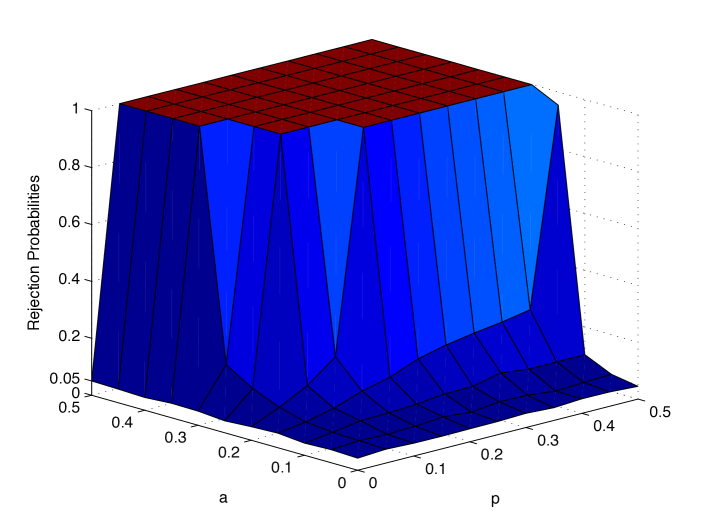
5.2 Statistical power

In the setting of Section 5.1 with $T=300$ and $N=100$, we study the statistical power of our testing procedure. For a certain proportion (say $p$) of the $N$ time series $\{X_{it}\}_{t=1}^{T}$ for $i\in\{1,\ldots,N\}$, we add a distortion $a\mu_{d}(t/T)$ in addition to (30), where $\mu_{d}(u)=2\cos(2\pi u)$ and $a$ denotes the corresponding magnitude. We investigate on the rejection probabilities at 5% nominal levels with different choices of $p$ and $a$ and the results are summarized in Figure 1. It can be easily seen that the power goes to one very quickly as the magnitude of distortion $a$ gets large and the proportion of different trends $p$ approaches 0.5.

Figure 1: Rejection probabilities at 5% nominal levels with different choices of deviation proportion $p$ and distortion magnitude $a$.

6 Application of the test to clustering

The test procedure developed in the previous sections can be applied to cluster collections of time series based on their similarity in terms of parallelism. In the sequel we identify the time series in (1) with their indexes. To build our iterative clustering algorithm, we start by finding the largest cluster $G_{1}$ in $U^{(0)}=\{1,\ldots,N\}$ for which the parallelism assumption $H_{0}$ is retained at level $\alpha$. The cluster $G_{1}$ is obtained by progressively removing from the analysis the sample units that contribute most to the test statistic (10). Specifically, $H_{0}$ is first tested on $U^{(0)}$, then on a subset $U^{(1)}\subset U^{(0)}$ if rejected on $U^{(0)}$, and so on so forth until $H_{0}$ is accepted or $U^{(k)}$ is reduced to a single element for some $k$, in which case the algorithm ends without any cluster being found. At the second iteration, the procedure is repeated with the remaining time series (set $U^{(0)}:=\{1,\ldots,N\}\setminus G_{1}$) and so on so forth until either all time series are clustered (i.e. $\{1,\ldots,N\}=G_{1}\cup\cdots\cup G_{L}$ for some $L$) or no more clusters of size $>1$ can be formed.

We now give a precise description of the algorithm. For the test implementation, the user must provide a significance level $\alpha$, bandwidth $b$ (cf. Sections 2 and 4.1), and parameters $(\tau,\varrho)$ (cf. Section 4.2). The user must also specify the number $n$ of sample units to remove at each step of the cluster search. As long as $n$ is small (say $n=1$ for small $N$ and, say $n\leq 5N/100=N/20$ for moderate to large $N$), this tuning parameter does not affect the outcome of the clustering algorithm; it however influences the computational time. Note that when moving from working index set $U^{(k)}$ to $U^{(k+1)}$ during the cluster search, the algorithm removes at least one and at most $(N_{k}-2)$ sample units from $U^{(k)}$, where $N_{k}$ is the size of $U^{(k)}$, so that there remains at least two units to compare at the next step. As a result the effective number of removed units is $n^{\ast}=\max(1,\min(n,N_{k}-2))$. Also, if $H_{0}$ is rejected on $U^{(k)}$ and accepted on $U^{(k+1)}$, this may mean that too many units ($n^{\ast}$ of them) have been removed from $U^{(k)}$ and that $H_{0}$ can be retained on an intermediate set $U^{(k+1)}\subseteq U^{\prime}\subset U^{(k)}$. In this case a flag $F$ is activated and the algorithm starts a dichotomic search, returning to the previous working index set $U^{(k)}$ and attempting to remove less units at each subsequent step (i.e. roughly $n/2$, then $n/4$, etc.). The following notations are needed for the formal statement of the algorithm:

• $k$: step counter; $l$: group counter, $F$: flag.

• $\bar{X}^{(k)}_{\cdot t}=N_{k}^{-1}\sum_{i\in U^{(k)}}X_{it}$, $\bar{X}_{\cdot\cdot}^{(k)}=T^{-1}\sum_{t=1}^{T}\bar{X}^{(k)}_{\cdot t}$, $\hat{\mu}^{(k)}(u)=\sum_{t=1}^{T}w_{b}(t,u)\bar{X}_{\cdot t}^{(k)}$, and $\hat{c}_{i}^{(k)}=T^{-1}\sum_{i\in U^{(k)}}\big{(}\hat{\mu}_{i}(t/T)-\hat{\mu}^{(k)}(t/T)\big{)}$. Recall that $N_{k}$ is the size of $U^{(k)}$.

The algorithm works as follows:

Initialization.

1. Set $U^{(0)}:=\{1,\ldots,N\}$, $k:=0$, $l:=1$, and $F:=0$.

2. Initialize the parameters $\alpha,b,\tau,\varrho,$ and $n$, with $n<N_{0}$.

3. Perform the parallelism test on $\{X_{it}\}_{t=1}^{T}$ for $i\in U^{(0)}$ and compute the $p$-value.

   1. Case $p>\alpha$.

      • Compute the $\Delta_{i}:=\int_{0}^{1}\big{\{}\hat{\mu}_{i}(u)-\hat{c}_{i}^{(0)}-\hat{\mu}^{(0)}(u)\big{\}}^{2}du$ for $i\in U^{(0)}$ and sort them as $\Delta_{\sigma(1)}\leq\cdots\leq\Delta_{\sigma(N_{0})}$.

      • Write $n^{\ast}:=\max(1,\min(n,N_{0}-2))$ and set

        $$U^{(1)}:=U^{(0)}\setminus\{\sigma(1),\ldots,\sigma(n^{\ast})\}\quad\textrm{and}\quad k:=1.$$

   2. Case $p\leq\alpha$.

      • Set $G_{1}:=U^{(0)}$ and stop the algorithm.

Determination of the cluster $G_{l}$.

1. If $N_{k}=1$, then stop the algorithm.

2. Perform the parallelism test on the $\{X_{it}\}_{t=1}^{T}$ for $i\in U^{(k)}$ and compute the $p$-value.

   1. Case $p>\alpha$.

      • Compute the $\Delta_{i}:=\int_{0}^{1}\big{\{}\hat{\mu}_{i}(u)-\hat{c}_{i}^{(k)}-\hat{\mu}^{(k)}(u)\big{\}}^{2}du$ for $i\in U^{(k)}$ and sort them as $\Delta_{\sigma(1)}\leq\cdots\leq\Delta_{\sigma(N_{k})}$.

      • If $F=1$, set $n:=\max(1,\lfloor n/2\rfloor)$.

      • Write $n^{\ast}:=\max(1,\min(n,N_{k}-2))$ and set

        $$U^{(k+1)}:=U^{(k)}\setminus\{\sigma(1),\ldots,\sigma(n^{\ast})\}\quad\textrm{and}\quad k:=k+1.$$

      • Return to step 4.

   2. Case $p\leq\alpha$.

      • Set $F:=1$.

      1. Case $n=1$.

         • Set $G_{l}:=U^{(k)}.$

         • If $\{1,\ldots,N\}=(G_{1}\cup\cdots\cup G_{l})$, then stop the algorithm.
           Else return to step 1 and set

           $$U^{(0)}:=\{1,\ldots,N\}\setminus(G_{1}\cup\cdots\cup G_{l}),\quad k:=0,\quad\textrm{and}\quad l:=l+1.$$

      2. Case $n>1$.

         • Set

           $$n:=\max(1,\lfloor n/2\rfloor)\quad\textrm{and}\quad U^{(k)}:=U^{(k-1)}\setminus\{\sigma(1),\ldots,\sigma(n^{\ast})\},$$

           where $n^{\ast}:=\max(1,\min(n,N_{k-1}-2))$.

         • Return to step 4.

The R implementation of the algorithm can be obtained from the authors upon request.

7 Analysis of Motorola data

To illustrate our parallelism test and clustering procedure, we consider a data set of hourly volumes of downloads from cell phones (in byte) in 129 U.S. area codes (24 area codes are in Center America, 87 in Eastern America, 1 in Hawaii, and 24 in Pacific America). Rather than studying the original data, we look into their daily sums so as to remove daily periodicity (which produces long-range dependence). Since the area codes have different numbers of phone users, we also apply a logarithmic transform (base 10) to the data to adjust for the scale effect. Thus, multiplicative differences in the time series become additive, which makes it relevant to test for parallelism in the trends of area codes. Examples of time series as well as the estimated global trend function $\mu=N^{-1}\sum_{i=1}^{N}\mu_{i}$ and long-run variance function $g$ are displayed in Figure 2.

Prior to statistical analysis, the validity conditions of our theoretical results have been verified on the data set. In particular, the rapid decrease observed in the autocorrelation functions of the detrended time series (see Figure 3) indicates that the short-range dependence assumption (19) is very plausible. Also global similarity in the autocovariance functions across the time series make the assumption of identically distributed error processes look reasonable. Finally, the $129\times 129$ cross-correlation matrix of the residual time series has nearly zero entries outside its diagonal, which suggests that the time series are independent.

Figure 2: Left panel: examples of download volume time series (daily-totaled and log-transformed) and estimated global trend in thick line. Right panel: Estimated long-run variance function.

Figure 3: Autocorrelation functions of the residual time series after a local linear fit with bandwidth $b=10$ days.

We now describe the implementation of the test and clustering algorithm on the data set. The significance level of the test is set to $5\%$. The local linear estimation of the trends is based on a bandwidth $b$ and a truncated standard Gaussian density. The inverse covariance matrix $\boldsymbol{\Gamma}^{-1}$ is estimated as in Section 4.1. Specifically, after a pilot trend estimation using a bandwidth $b=5$ days, the “banding the inverse covariance matrix” technique (e.g. Bickel and Levina (2008)) has been applied to the sample covariance matrix of residuals with a banding parameter $k=6$ days. The final bandwidth $b$ is obtained by minimizing the GCV score (22). The long-run variance function $g$ is estimated as in Section 4.2 based on the residuals of a local linear smoothing with bandwidth $b=10$. (A larger $b$ is used to estimate the long-run variance function than for the trend estimation so as to make the estimate less sensitive to extreme observations.) The parameters $\tau=0.04$ and $\varrho=0.31$ are chosen so that the estimate of $g(u),u\in[0,1]$ utilizes about 2 weeks of data before and after a time point $u$ and the autocovariances are truncated at lag $K_{T}=4$. These parameter values are based on the visual inspection of the autocovariance plots. Finally the number $n$ of units to remove at each step of the cluster search (see Section 6) is set to 3, a good compromise between search accuracy and computational speed of the algorithm.

The results of the analysis are presented in Tables 2 and 3. Note that performing the parallelism test on the entire data set resulted in a $p$-value $<10^{-16}$. Shifting our focus to clustering the time series, we observe that the four largest clusters found contain respectively 29, 21, 20, and 10 area codes. This alone represents a sizable proportion (62%) of the 129 area codes under study. These clusters are displayed in Figure 4, where their homogeneity can be observed. The examination of Table 3 reveals that there is no obvious spatial pattern in the clusters. It also shows that there is no systematic relation between the size of a cluster and its associated $p$-value. Overall, our statistical analysis shows that most area codes under study can be classified in a small number of profiles, or clusters, according to the parallelism patterns in their phone download activity. These strong similarities across area codes would deserve to be investigated in more detail as potentially, they could be exploited by phone companies to e.g. better target their marketing strategies or improve the bandwidth allocation.

Figure 4: Trends in the clusters of size $s\geq 10$. After a log-transform of the data, the trends are obtained by smoothing the time series with a bandwidth $b=4$ days.

Cluster size	29	21	20	10	7	5	3	2	1
# clusters	1	1	1	1	1	1	2	7	17
cum. prop. of $N$	22%	39%	54%	62%	67%	71%	76%	87%	100%

Table 2: Summary of the clusters. The clusters are maximal sets of area codes for which the parallelism assumption is retained at the significance level 5%.

Cluster 1: size 29, p-value 0.095

code	state	code	state	code	state	code	state	code	state	code	state
203	CT	321	FL	517	MI	617	MA	810	MI	909	CA
219	IN	323	CA	540	VA	619	CA	813	FL	941	FL
239	FL	484	PA	562	CA	646	NY	815	IL	951	CA
301	MD	508	MA	603	NH	661	CA	856	NJ	978	MA
302	DE	513	OH	616	MI	703	VA	859	KY

Cluster 2: size 21, p-value 0.064

code	state	code	state	code	state	code	state	code	state	code	state
209	CA	586	MI	630	IL	732	NJ	781	MA	908	NJ
240	MD	609	NJ	631	NY	734	MI	786	FL
510	CA	610	PA	708	IL	772	FL	818	CA
561	FL	626	CA	714	CA	774	MA	845	NY

Cluster 3: size 20, p-value 0.151

code	state	code	state	code	state	code	state	code	state
231	MI	404	GA	512	TX	803	SC	904	FL
269	MI	407	FL	704	NC	816	MO	919	NC
352	FL	412	PA	740	OH	863	FL	937	OH
386	FL	419	OH	773	IL	864	SC	989	MI

Cluster 4: size 10, p-value 0.071

code	state	code	state	code	state	code	state	code	state
248	MI	570	PA	805	CA	847	IL	916	CA
516	NY	571	VA	808	HI	914	NY	917	NY

Table 3: Spatial locations of clusters. Only clusters of size $s\geq 10$ are displayed.

8 Conclusion

In this paper we have presented a test methodology for assessing the parallelism between trends of multiple time series. The physical dependence structure considered here allows to flexibly model nonstationary time series without having to specify some generating mechanism or autocovariance function. A method for estimating the long-run variance function of locally stationary processes and a simulation-based device to approximate the distribution of statistics based on smoothed time series have been developed as by-products of the test methodology. Both these tools have shown good numerical performances in our simulations. They are of independent interest and could be used with profit in other statistical problems. A key assumption used to derive the theory of this paper is that the observed time series are independent from one another. A very interesting extension would be to allow for some form of dependence, e.g. to handle spatio-temporal data.

The paper also proposes an innovative method to cluster time series according to their parallelism properties. This method has at least two attractive features: first, it does not require to prespecify the number of clusters to be found, which guarantees the homogeneity of the clusters and allows atypical time series to be set apart; second, it readily provides significance levels for each cluster, thereby giving a quantitative sense of how strong the parallelism assumption holds. The implementation of this clustering method has given meaningful results with the Motorola time series. The algorithm is computationally fast as the individual trend functions and long-variance functions need being estimated only once, while the most computationally intensive step (Gaussian process simulation to approximate the distribution of the test statistic) is still manageable. The ideas harnessed in this algorithm (greedy search, clustering based on individual contribution of sample units to test statistic) can be used to cluster time series according to other similarity measures than parallelism. An interesting direction of future research would be to compare the results of this type of clustering to the more conventional $k$-means or hierarchical approaches.

9 Appendix

In the proofs we use $C$ to denote a constant whose value may vary from place to place. It does not depend on $N$ and $T$.

9.1 Proof of Theorem 1

The techniques for handling Case (i) with large $N$ and Case (ii) with fixed $N$ are different. For the former we apply the traditional Lindeberg-Feller CLT, while for the latter, we apply the $m$-dependence and martingale approximation techniques. For details see Sections 9.1.1 and 9.1.2, respectively.

We start by showing that under $H_{0}$, the test statistic $\widehat{\Delta}_{N,T}$ does not depend upon $\mu(\cdot)$ nor the $c_{i}$. To see this, introduce the weight averages

$$\bar{w}_{b}(t)=T^{-1}\sum_{j=1}^{T}w_{b}(t,j/T)$$

With (5), (8), and (9), we easily see that

$$\hat{\mu}_{i}(u)-\hat{\mu}(u)-\hat{c}_{i} =\sum_{t=1}^{T}\left(w_{b}(t,u)-\bar{w}_{b}(t)\right)\left(c_{i}+e_{it}-\bar{e}_{\cdot t}\right)$$

$$=\sum_{t=1}^{T}\left\{w_{b}(t,u)-\bar{w}_{b}(t)\right\}\left(e_{it}-\bar{e}_{\cdot t}\right).$$

The last equality stems from the fact that $\sum_{t=1}^{T}\left[w_{b}(t,u)-\bar{w}_{b}(t)\right]=1-1=0$ by the well known property that the weight functions $w_{b}(t,\cdot),t=1,\ldots,T,$ of the local linear smoother sum up to one.

9.1.1 Case (i): $N\to\infty$

We shall prove the asymptotically equivalent form of (20)

$$Tb^{1/2}N^{-1/2}(\widehat{\Delta}_{N,T}-{\tenopen\mathbb{E}}\widehat{\Delta}_{N,T})\mathop{\rightarrow}^{\mathcal{L}}N(0,\sigma^{2}K_{2}^{*}).$$ (32)

To this end, we use the decomposition

$$\widehat{\Delta}_{N,T}-{\tenopen\mathbb{E}}\widehat{\Delta}_{N,T}=\sum_{i=1}^{N}(A_{i}-{\tenopen\mathbb{E}}A_{i})-\left(R_{N}-{\tenopen\mathbb{E}}R_{N}\right)$$ (33)

where

$$A_{i}=\int_{0}^{1}\Big{(}\sum_{t=1}^{T}\left(w_{b}(t,u)-\bar{w}_{b}(t)\right)e_{it}\Big{)}^{2}du$$

$$\textrm{and}\quad R_{N}=N\int_{0}^{1}\Big{(}\sum_{t=1}^{T}\left(w_{b}(t,u)-\bar{w}_{b}(t)\right)\bar{e}_{\cdot t}\Big{)}^{2}du,$$

and we show that asymptotically, $\sum_{i}A_{i}$ is normally distributed and $R_{N}$ is negligible.

First, define

$$A_{i}^{\circ}=\int_{0}^{1}\Big{(}\sum_{t=1}^{T}w_{b}(t,u)e_{it}\Big{)}^{2}du.$$

By Theorem 1 in Zhang and Wu (2011), under the bandwidth conditions $Tb^{3/2}\to\infty$ and $b\to 0$ and the short-range dependence condition (19), we have

$$Tb^{1/2}\left(A^{\circ}_{i}-{\tenopen\mathbb{E}}A^{\circ}_{i}\right)\mathop{\rightarrow}^{\mathcal{L}}N(0,\sigma^{2}K_{2}^{*}).$$ (34)

Observing that $A^{\circ}_{1},\ldots,A^{\circ}_{N}$ are i.i.d., it results from (34) and the Lindeberg-Feller CLT that

$${Tb^{1/2}\over\sqrt{N}}\sum_{i=1}^{N}\left(A^{\circ}_{i}-{\tenopen\mathbb{E}}A_{i}^{\circ}\right)\mathop{\rightarrow}^{\mathcal{L}}N(0,\sigma^{2}K_{2}^{*}).$$ (35)

We now show that $Tb^{1/2}N^{-1/2}\sum_{i=1}^{N}(A_{i}^{\circ}-A_{i})$ is negligible as $N,T\to\infty$. Let

$$J_{i}=\sum_{t=1}^{T}\bar{w}_{b}(t)e_{it}\>\>\textrm{and}\>\>\dot{J}_{i}=\sum_{t=1}^{T}\dot{w}_{b}(t)e_{it},\quad\textrm{where}\>\>\dot{w}_{b}(t)=\int_{0}^{1}w_{b}(t,u)du.$$

Noting that $\max_{t}|\bar{w}_{b}(t)|=O(T^{-1})$ and $\max_{t}|\dot{w}_{b}(t)|=O(T^{-1})$, one can obtain from Lemma 1 in Liu and Wu (2010) that $\|J_{i}\|_{4}=O(T^{-1/2})$ and $\|\dot{J}_{i}\|_{4}=O(T^{-1/2})$. Hence,

$$\left\|A_{i}^{\circ}-A_{i}\right\|_{2}^{2}=\|J_{i}^{2}-2J_{i}\dot{J}_{i}\|_{2}^{2}=O(T^{-2})$$ (36)

and by the i.i.d. character of the $(A_{i}^{\circ}-A_{i})$, one deduces that

$$\bigg{\|}Tb^{1/2}N^{-1/2}\sum_{i=1}^{N}(A_{i}^{\circ}-A_{i})\bigg{\|}_{2}^{2}=O(b).$$ (37)

We proceed to study the remainder term $(R_{N}-{\tenopen\mathbb{E}}R_{N})$ in (33). By expanding $R_{N}$ and using the i.i.d. character of the $N$ time series, one easily finds that

$$R_{N}\stackrel{{\scriptstyle d}}{{=}}A_{1}^{\circ}+J_{1}^{2}-2J_{1}\dot{J}_{1},$$ (38)

where $\stackrel{{\scriptstyle d}}{{=}}$ stands for equality in distribution. The terms in the above expansion have been studied before. More precisely, the relations (34) and (36) yield

$$\big{\|}Tb^{1/2}N^{-1/2}\left(R_{N}-{\tenopen\mathbb{E}}R_{N}\right)\big{\|}_{2}^{2}=O(N^{-1})+O(N^{-1}b).$$ (39)

Putting together (33), (35), (37), and (39), one obtains the asymptotic normality (32).

9.1.2 Case (ii): $N$ is fixed

Recall that $e_{it}=G(t/T;\mathcal{F}_{it})$. For $\zeta_{it}(u)=G(u;\mathcal{F}_{it})$, define

$$\tilde{\zeta}_{it}(u)=\mathbb{E}(\zeta_{it}(u)|\varepsilon_{i,t-m+1},\varepsilon_{i,t-m+2},\ldots,\varepsilon_{i,t}).$$

Then the process $\{\tilde{\zeta}_{it}(u)\}_{t\in{\tenopen\mathbb{Z}}}$ is $m$-dependent with long-run variance function $g^{\ast}$ converging to $g$ as $m\to\infty$. As in the proof of Theorem 1 in Zhang and Wu (2011), we introduce the martingale difference

$$\tilde{D}^{*}_{i,t} = \sum_{l=0}^{\infty}\mathbb{E}(\tilde{\zeta}_{i,t+l}(t/T)|{\cal F}_{it})-\mathbb{E}(\tilde{\zeta}_{i,t+l}(t/T)|{\cal F}_{i,t-1})$$

$$= \sum_{l=0}^{m}\mathbb{E}(\tilde{\zeta}_{i,t+l}(t/T)|{\cal F}_{it})-\mathbb{E}(\tilde{\zeta}_{i,t+l}(t/T)|{\cal F}_{i,t-1}).$$

Observe that $\tilde{D}^{*}_{i,t}$, $1\leq t\leq T$, are also $m$-dependent. Let $\tilde{D}^{\dagger}_{i,t}=\tilde{D}^{*}_{i,t}-\tilde{D}^{*}_{\cdot,t}$, where $\tilde{D}^{*}_{\cdot,t}=\sum_{i=1}^{N}\tilde{D}^{*}_{i,t}/N$; let $(\sigma^{\ast})^{2}=\int_{0}^{1}(g^{\ast}(u))^{2}du$. By the argument of Theorem 1 in Zhang and Wu (2011), to derive the asymptotic normality $\eqref{eq:cltallN}$, it suffices to show that as $T\to\infty$,

$$\frac{1}{T^{2}b(N-1)}\sum_{1\leq t<t^{\prime}\leq T}\Big{(}K^{*}\Big{(}\frac{t-t^{\prime}}{2Tb}\Big{)}\Big{)}^{2}\sum_{i=1}^{N}\sum_{i^{\prime}=1}^{N}\mathbb{E}(\tilde{D}^{\dagger}_{i,t}\tilde{D}^{\dagger}_{i^{\prime},t})\mathbb{E}(\tilde{D}^{\dagger}_{i,t^{\prime}}\tilde{D}^{\dagger}_{i^{\prime},t^{\prime}})\to K_{2}^{*}(\sigma^{\ast})^{2}.$$ (40)

Since the $\tilde{D}^{\dagger}_{i,t}$, $i=1,\ldots,N$, are i.i.d., we see that $\mathbb{E}(\tilde{D}^{\dagger}_{i,t}\tilde{D}^{\dagger}_{i^{\prime},t})=g^{\ast}(t)(N-1)/N$ if $i=i^{\prime}$ and $\mathbb{E}(\tilde{D}^{\dagger}_{i,t}\tilde{D}^{\dagger}_{i^{\prime},t})=-g^{\ast}(t)/N$ if $i\neq i^{\prime}$. With a few manipulations, we then obtain

$$\sum_{i=1}^{N}\sum_{i^{\prime}=1}^{N}\mathbb{E}(\tilde{D}^{\dagger}_{i,t}\tilde{D}^{\dagger}_{i^{\prime},t})\mathbb{E}(\tilde{D}^{\dagger}_{i,t^{\prime}}\tilde{D}^{\dagger}_{i^{\prime},t^{\prime}})=(N-1)g^{\ast}(t)g^{\ast}(t^{\prime}).$$

Furthermore, with the continuity of $g^{\ast}$, classic arguments for kernel smoothing show that

$$\frac{1}{T^{2}b}\sum_{1\leq t<t^{\prime}\leq T}\Big{(}K^{*}\Big{(}\frac{t-t^{\prime}}{2Tb}\Big{)}\Big{)}^{2}g^{\ast}(t)g^{\ast}(t^{\prime})=K_{2}^{*}(\sigma^{\ast})^{2}+o(1).$$

Hence (40) is proved and the asymptotic normality (20) follows. $\square$

9.2 Proof of Theorem 2

By (33) and the Cauchy-Schwarz inequality, we can write

$$\widehat{\Delta}_{N,T}=I_{N,T}+\Big{(}\sum_{i=1}^{N}A_{i}-R_{N}\Big{)}+\mathcal{O}_{p}\left(I_{N,T}^{1/2}\Big{(}\sum_{i=1}^{N}A_{i}-R_{N}\Big{)}^{1/2}\right),$$ (41)

where

$$I_{N,T}=\sum_{i=1}^{N}\int_{0}^{1}\Big{\{}\sum_{t=1}^{T}\left(w_{b}(t,u)-\bar{w}_{b}(t)\right)\left(\mu_{i}(t/T)-\mu(t/T)\right)\Big{\}}^{2}du$$

and $\mu=N^{-1}\sum_{i=1}^{N}\mu_{i}$. By the approximation properties of local linear smoothers (see for example Proposition 1.13 in p.39 of Tsybakov (2009)), we obtain

$$I_{N,T}=\Delta_{N}+\mathcal{O}\left(N(b^{2}+T^{-1})\right),$$ (42)

provided that the $\mu_{i},i=1,\ldots,N,$ have uniformly bounded second derivatives on $[0,1]$.

On the other hand, we know from (35), (37), and (39) that

$$Tb^{1/2}N^{-1/2}\Big{(}\sum_{i=1}^{N}\left(A_{i}-{\tenopen\mathbb{E}}A_{i}\right)-R_{N}\Big{)}\mathop{\rightarrow}^{\mathcal{L}}N(0,\sigma^{2}K_{2}^{*}).$$ (43)

By the stochastic Lipschitz continuity (14) and the short-range dependence condition (19), and by properties of weight functions of local linear smoothers (see Lemma 1.3 in p.38 of Tsybakov (2009)) we also have ${\tenopen\mathbb{E}}A_{i}=\mathcal{O}((Tb)^{-1})$. Hence,

$$\widehat{\Delta}_{N,T}=\Delta_{N}+\mathcal{O}\left(Nb^{2}\right)+\mathcal{O}\left(N/Tb\right)+o_{P}\left(N/Tb\right).$$ (44)

If $N^{-1}\Delta_{N}$ converges to 0 at a rate slower than $b^{2}+1/Tb$, then $N^{-1}(b^{2}+1/Tb)\hat{\Delta}_{N,T}\to\infty$ in probability. Hence the test based on $\hat{\Delta}_{N,T}$ has unit asymptotic power. $\square$

9.3 Proof of Theorem 3

Let $\hat{g}_{i}(u)=\sum_{k=-K_{T}}^{K_{T}}\hat{\gamma}_{ik}(u)$ be the estimated long-run variance based on $\{e_{it}\}_{t=1}^{T}$, where $K_{T}=\lfloor T\tau\varrho\rfloor$ is the truncation order and $\hat{\gamma}_{ik}=\frac{1}{|\mathcal{N}_{\tau}(u)|-|k|}\sum_{t,t+k\in\mathcal{N}_{\tau}(u)}e_{it}e_{i,t+k}$ is the sample autocovariance at lag $k$. Since the cardinality $|N_{\tau}(u)|$ is of order $T\tau$, one sees that

$$\hat{g}_{i}(u)=\frac{1+\mathcal{O}(\varrho)}{|\mathcal{N}_{\tau}(u)|}\sum_{t\in\mathcal{N}_{\tau}(u)}\sum_{t^{\prime}\in\mathcal{N}_{\tau}(u)}e_{it}e_{it^{\prime}}1{\hskip-3.0pt}\hbox{I}_{\{|t-t^{\prime}|\leq K_{T}\}}\,.$$ (45)

By the argument of Proposition 1 in Liu and Wu (2010), it can be shown that $\sup_{u\in\left[0,1\right]}\|\hat{g}_{i}(u)-\mathbb{E}\hat{g}_{i}(u)\|_{2}=\mathcal{O}(\sqrt{\varrho})$ and by the i.i.d. property of the $\{e_{it}\}_{t=1}^{T}$, one deduces that

$$\sup_{u\in\left[0,1\right]}\|\hat{g}(u)-\mathbb{E}\hat{g}(u)\|_{2}=\mathcal{O}(\sqrt{\varrho/N}).$$ (46)

The expectation ${\tenopen\mathbb{E}}\hat{g}_{i}(u)$ can be used to approximate the truncation of $g(u)$ to order $K_{T}$ thanks to the stochastic Lipschitz continuity (14) and the martingale decomposition of Wu (2007). Specifically, let $\Gamma_{2}(k)=\sum_{j=0}^{\infty}\delta_{2}(j)\delta_{2}(j+k)$. Then for all $u\in[0,1]$ and $t,t^{\prime}\in\mathcal{N}_{\tau}(u)$ such that $|t-t^{\prime}|\leq K_{T}$, it holds that

$$\left|\mathbb{E}(e_{it}e_{it^{\prime}})-\gamma_{|t-t^{\prime}|}(t/T)\right|\leq C(\Gamma_{2}(|t-t^{\prime}|)\wedge(\tau\varrho)).$$ (47)

Moreover, we obtain after easy calculation that

$$\sum_{k=0}^{\infty}(\Gamma_{2}(k)\wedge(\tau\varrho))=\mathcal{O}((\tau\varrho)^{\alpha/(1+\alpha)}).$$ (48)

Taking the expectation in (45) and adding terms so that the summation index set is $\{(t,t^{\prime}):t\in\mathcal{N}_{\tau}(u),1\leq t^{\prime}\leq T,|t-t^{\prime}|\leq K_{T}\}$, it stems from (47) and (48) that

$${\tenopen\mathbb{E}}\hat{g}_{i}(u) =\frac{1+\mathcal{O}(\varrho)}{|\mathcal{N}_{\tau}(u)|}\bigg{(}\sum_{t\in\mathcal{N}_{\tau}(u)}\sum_{t^{\prime}=1}^{T}\mathbb{E}(e_{it}e_{it^{\prime}})1{\hskip-3.0pt}\hbox{I}_{\{|t-t^{\prime}|\leq K_{T}\}}+\mathcal{O}(K_{T})\bigg{)}$$

$$=\frac{1}{|\mathcal{N}_{\tau}(u)|}\sum_{t\in\mathcal{N}_{\tau}(u)}\sum_{k=-K_{T}}^{K_{T}}{\tenopen\mathbb{E}}e_{it}e_{i,t+k}+\mathcal{O}(\varrho)$$

$$=\frac{1}{|\mathcal{N}_{\tau}(u)|}\sum_{t\in\mathcal{N}_{\tau}(u)}\sum_{k=-K_{T}}^{K_{T}}\gamma_{k}(t/T)+\mathcal{O}((\tau\varrho)^{\alpha/(1+\alpha)})+\mathcal{O}(\varrho)$$

$$=\frac{1}{|\mathcal{N}_{\tau}(u)|}\sum_{t\in\mathcal{N}_{\tau}(u)}\Big{(}g(t/T)-2\sum_{k=K_{T}}^{\infty}\gamma_{k}(t/T)\Big{)}+\mathcal{O}((\tau\varrho)^{\alpha/(1+\alpha)})+\mathcal{O}\left(\varrho\right).$$ (49)

In (9.3), a Taylor expansion of $g\in\mathcal{C}^{2}[0,1]$ at order 2 yields

$$\sup_{u\in[0,1]}\bigg{|}\frac{1}{|\mathcal{N}_{\tau}(u)|}\sum_{t\in\mathcal{N}_{\tau}(u)}g(t/T)-g(u)\bigg{|}=\mathcal{O}(\tau^{2}).$$ (50)

Also, the martingale decomposition of Wu (2007) can be applied to show that $\sup_{u\in[0,1]}|\gamma_{k}(u)|\leq\Gamma_{2}(k)$, so that under the assumptions of Theorem 2,

$$\sup_{u\in[0,1]}\sum_{k=K_{T}}^{\infty}|\gamma_{k}(u)|=\mathcal{O}\bigg{(}\sum_{k=K_{T}}^{\infty}\delta_{2}(k)\bigg{)}=\mathcal{O}\left((T\tau\varrho)^{-\alpha}\right).$$ (51)

Finally, to obtain (28), it suffices to note that $\mathbb{E}\hat{g}(u)=\mathbb{E}\hat{g}_{i}(u)$.

To derive (29), an easy calculation shows that

$$\tilde{g}_{i}(u)-\hat{g}_{i}(u) = {2\over|\mathcal{N}_{\tau}(u)|}\sum_{t\in\mathcal{N}_{\tau}(u)}\sum_{t^{\prime}\in\mathcal{N}_{\tau}(u)}(\hat{e}_{it}-e_{it})e_{it^{\prime}}1{\hskip-3.0pt}\hbox{I}_{\{|t-t^{\prime}|\leq K_{T}\}}$$

$$+{1\over|\mathcal{N}_{\tau}(u)|}\sum_{t\in\mathcal{N}_{\tau}(u)}\sum_{t^{\prime}\in\mathcal{N}_{\tau}(u)}(\hat{e}_{it}-e_{it})(\hat{e}_{it^{\prime}}-e_{it^{\prime}})1{\hskip-3.0pt}\hbox{I}_{\{|t-t^{\prime}|\leq K_{T}\}}$$

$$:= I_{N,T}(u)+I\negthinspace I_{N,T}(u).$$

Noticing that $\hat{e}_{it}-e_{it}=\beta_{i}(t/T)-\sum_{t^{\prime\prime}=1}^{T}\beta_{i}(t^{\prime\prime}/T)w_{b}(t^{\prime\prime},t)-\sum_{t^{\prime\prime}=1}^{T}e_{it^{\prime\prime}}w_{b}(t^{\prime\prime},t)$, we have

$$\max_{t=1,\ldots,T}\|\hat{e}_{it}-e_{it}\|_{p}\leq C(b^{2}+T^{-1/2}b^{-1/2}).$$

Hence by Lemma 1 in Zhang and Wu (2011), we have $\sup_{u\in[0,1]}\|I_{N,T}(u)\|_{p}\leq C\iota$ and $\sup_{u\in[0,1]}\|I\negthinspace I_{N,T}(u)\|_{p}\leq C\iota^{2}$, which proves (29). $\square$

References

Bickel and Levina (2008). Regularized estimation of large covariance matrices. Ann. Statist. 36, 199–227.

Bissantz, N., Holzmann, H., and Munk, A. (2005). Testing parametric assumptions on band- or time-limited signals under noise. IEEE Trans. Inform. Theory 51, 3796–3805.

Degras, D. (2010). Simultaneous confidence bands for nonparametric regression with functional data. Statist. Sinica, To appear. Available at http://arxiv.org/abs/0908.1980

Delgado, M. A. (1993). Testing the equality of nonparametric regression curves. Stat. Probab. Lett. 17, 199–204.

Fan, J. and Lin, S. K. (1998). Test of significance when data are curves. J. Amer. Statist. Assoc. 93, 1007–1021.

Fan, J. and Gijbels, I. (1996). Local Polynomial Modeling and its Applications. London, U.K.: Chapman & Hall.

Gottschalk, P. G. and Dunn, J. R. (2005). Measuring parallelism, linearity, and relative potency in bioassay and immunoassay data. J. Biopharm. Statist. 15, 437–463.

Guo, P. and Oyet, A. J. (2009). On wavelet methods for testing equality of mean response curves. Int. J. Wavelets Multiresolut. Inf. Process. 7, 357–373.

Hall, P. and Hart, J.D. (1990). Bootstrap test for difference between means in nonparametric regression. J. Amer. Statist. Assoc. 85, 1039–1049.

Härdle, W. and Marron, J. S. (1990). Semiparametric comparison of regression curves. Ann. Statist. 18, 63–89.

Härdle, W. and Mammen, E. (1993). Comparing nonparametric versus parametric regression fits. Ann. Statist. 21, 1926–1947.

Lavergne, P. (2001). An equality test across nonparametric regressions. J. Econometrics 103, 307–344.

Li, F. (2006). Testing for the equality of two nonparametric regression curves with long memory errors. Comm. Statist. Simulation Comput. 35, 621–643.

Liu, W. D. and Wu, W. B. (2010). Asymptotics of spectral density estimates. Econometric Theory 26, 1218–1245.

King, E. C., Hart, J. D. and Wehrly, T. E. (1991). Testing the equality of regression curves using linear smoothers. Statist. Probab. Lett. 12, 239–247.

Koul, H. L. and Schick, A. (1997). Testing for the equality of two nonparametric regression curves. J. of Statist. Plann. Inf. 65, 293–314.

Munk, A. and H. Dette (1998). Nonparametric comparison of several regression functions: exact and asymptotic theory. Ann. Statist., 6 2339–2368.

Orbe, S., Ferreira, E. and Rodriguez-Poo, J. (2005) Nonparametric estimation of time varying parameters under shape restrictions. J. Econometr., 126 53–77.

Park, C., Vaughan, A., Hannig, J. and Kang, K. H. (2009). SiZer analysis for the comparison of time series. J. Statist. Plann. Inf. 139, 3974–3988.

Pawlak, M. and Stadtmüller, U. (2007) Signal Sampling and Recovery Under Dependent Errors, IEEE Trans. Inf. Theory 53, 2526–2541.

Vilar-Fernandez J. M., Vilar-Fernandez J. A., and Gonzalez-Manteiga W. (2007). Bootstrap tests for nonparametric comparison of regression curves with dependent errors. Test 16, 123–144.

Tsybakov A. B. (2009). Introduction to nonparametric estimation. Springer, New York.

Wu, W. B. (2005). Nonlinear system theory: another look at dependence. Proc. Natl Acad. Sci. USA 102, 14150–14154.

Wu, W. B. (2007). Strong invariance principles for dependent random variables. Ann. Prob. 35, 2294–2320.

Wu, W. B. and Zhao, Z. (2007) Inference of Trends in Time Series. Journal of the Royal Statistical Society, Series B, 69 391–410

Wu, W. B. and Zhou, Z. (2011). Gaussian approximations for non-stationary multiple time series. Statist. Sinica, To appear.

Young, S. G. and Bowman, A.W. (1995). Non-parametric analysis of covariance. Biometrics, 51 920–931.

Zhang, T. and Wu, W. B. (2011). Testing parametric assumptions of trends of non-stationary time series. Biometrika, To appear.