Nonleptonic $B_{s}$ to charmonium decays and their role in the determination of the $\beta_{s}$

Abstract

This talk consists of two parts. We first present a light-cone QCD sum rule computation of the $B_{s}\to f_{0}(980)$ form factors which are necessary inputs in semileptonic and nonleptonic $B_{s}$ decays into $f_{0}(980)$. Then we analyze nonleptonic $B_{s}$ decays into a charmonium state and a light meson, which are potentially useful to access the $B_{s}$-${\bar{B}}_{s}$ mixing phase $\beta_{s}$. We explore the experimental feasibility of measuring these various channels, paying attention to different determinations of $\beta_{s}$ in view of the hints of new physics recently emerged in the $B_{s}$ sector.

1 Introduction

The detailed study of CP violation is a powerful and rigorous tool in the discrimination between the Standard Model (SM) and alternative scenarios. For instance the analysis of the $B_{s}$ unitarity triangle of the Cabibbo-Kobayashi-Maskawa (CKM) matrix elements: $V_{us}V_{ub}^{*}+V_{cs}V_{cb}^{*}+V_{ts}V_{tb}^{*}=0$ provides an important test of the SM description of CP violation. One of its angles, defined as $\beta_{s}=Arg\big{[}-{V_{ts}V_{tb}^{*}\over V_{cs}V_{cb}^{*}}\big{]}$, is half of the phase in the $B_{s}$-${\bar{B}}_{s}$ mixing, and is expected to be tiny in the SM: $\beta_{s}\simeq 0.017$ rad. The current measurements, by the CDF and DØ collaborations at Tevatron based on the angular analysis of the time-dependent differential decay width in the process $B_{s}\to J/\psi\phi$ :2008fj , indicate larger values and the averaged results are consistent with SM only at 2.2 $\sigma$ level: $\phi_{s}^{J/\psi\phi}=-2\beta_{s}=-0.77\pm^{0.29}_{0.37}$ or $\phi_{s}^{J/\psi\phi}=-2\beta_{s}=-2.36\pm^{0.37}_{0.29}$ Barberio:2008fa . Although the recent result by the CDF: $\beta_{s}\in[0.0,0.5]\,{\rm U}\,[1.1,1.5]$ (at 68$\%$ confidence level) talkcdf has a smaller deviation from the SM, the uncertainties are still large and the precise measurement of $\beta_{s}$ is a priority for the forthcoming experiments. Towards this direction the nonleptonic $B_{s}$ decays are certainly of prime importance.

In this work we first compute the $B_{s}\to f_{0}(980)$ form factors using the light-cone QCD sum rule (LCSR)Colangelo:2010bg . These results will be useful in the analysis of semileptonic and nonleptonic $B_{s}\to f_{0}$ decays. Subsequently we investigate the $B_{s}$ decay modes induced by the transition $b\to c{\bar{c}}s$, namely $B_{s}\to M_{c{\bar{c}}}+L$, where $M_{c{\bar{c}}}$ is an s-wave or p-wave charmonium state and $L$ is a light scalar, pseudoscalar or vector meson, $f_{0}(980)$, $\eta$, $\eta^{\prime}$, $\phi$ Colangelo:2010zz . In particular, we exploit the generalized factorization approach to calculate their branching fractions in the SM in order to understand which of these modes are better suitable to determine $\beta_{s}$.

2 $B_{s}\to f_{0}$ form factors in LCSR

Hereafter we will use $f_{0}$ to denote $f_{0}(980)$ meson for simplicity. The parametrization of matrix elements involved in $B_{s}\to f_{0}$ transitions is expressed in terms of the form factors

$$\langle f_{0}(p_{f_{0}})|J^{5}_{\mu}|\overline{B}_{s}(p_{B_{s}})\rangle=-i\big{\{}F_{1}(q^{2})\big{[}P_{\mu}-\frac{m_{B_{s}}^{2}-m_{f_{0}}^{2}}{q^{2}}q_{\mu}\big{]}+F_{0}(q^{2})\frac{m_{B_{s}}^{2}-m_{f_{0}}^{2}}{q^{2}}q_{\mu}\big{\}},$$

$$\langle{f_{0}}(p_{f_{0}})|J_{\mu}^{5T}|\overline{B}_{s}(p_{B_{s}})\rangle=-\frac{F_{T}(q^{2})}{m_{B_{s}}+m_{f_{0}}}\Big{[}q^{2}P_{\mu}-(m_{B_{s}}^{2}-m_{f_{0}}^{2})q_{\mu}\Big{]},$$ (1)

where $P=p_{B_{s}}+p_{f_{0}}$, $q=p_{B_{s}}-p_{f_{0}}$, and $J_{\mu}^{5}=\bar{s}\gamma_{\mu}\gamma_{5}b$, $J_{\mu}^{5T}=\bar{s}\sigma_{\mu\nu}\gamma_{5}q^{\nu}b$ . To compute such form factors in the LCSR Colangelo:2000dp we consider the correlation function:

$$\Pi(p_{f_{0}},q)=i\int d^{4}x\,e^{iq\cdot x}\langle{f_{0}}(p_{f_{0}})|{\rm T}\left\{j_{\Gamma_{1}}(x),j_{\Gamma_{2}}(0)\right\}|0\rangle$$ (2)

with $j_{\Gamma_{1}}$ being one of the currents in the definition of the $B_{s}\to f_{0}$ form factors: $j_{\Gamma_{1}}=J_{\mu}^{5}$ for $F_{1}$ and $F_{0}$, and $j_{\Gamma_{1}}=J_{\mu}^{5T}$ for $F_{T}$. The matrix element of $j_{\Gamma_{2}}=\bar{b}i\gamma_{5}s$ between the vacuum and $B_{s}$ defines the $B_{s}$ decay constant $f_{B_{s}}$ : $\langle\overline{B}_{s}(p_{B_{s}})|\bar{b}i\gamma_{5}s|0\rangle=\frac{m_{B_{s}}^{2}}{m_{b}+m_{s}}f_{B_{s}}$.

The LCSR method consists in evaluating the correlation function in Eq. (2) both at the hadron level and at the quark level. Equating the two representations allows us to obtain a set of sum rules suitable to derive the form factors.

The hadronic representation of the correlation function in Eq.  (2) can be written as the sum of the contribution of the $\bar{B}_{s}$ state and that of the higher resonances and the continuum of states $h$:

$$\Pi^{\rm H}(p_{f_{0}},q)=\frac{\langle{f_{0}}(p_{f_{0}})|j_{\Gamma_{1}}|\overline{B}_{s}(p_{f_{0}}+q)\rangle\langle\overline{B}_{s}(p_{f_{0}}+q)|j_{\Gamma_{2}}|0\rangle}{m_{B_{s}}^{2}-(p_{f_{0}}+q)^{2}}+\int_{s_{0}}^{\infty}ds\frac{\rho^{h}(s,q^{2})}{s-(p_{f_{0}}+q)^{2}},$$ (3)

where higher resonances and the continuum of states are described in terms of the spectral function $\rho^{h}(s,q^{2})$, contributing above a threshold $s_{0}$.

The correlation function can be evaluated in QCD with the expression

$$\Pi^{\rm QCD}(p_{f_{0}},q)=\frac{1}{\pi}\int_{(m_{b}+m_{s})^{2}}^{\infty}ds\,\frac{{\rm Im}\Pi^{\rm QCD}(s,q^{2})}{s-(p_{f_{0}}+q)^{2}}\,.$$ (4)

Expanding the T-product in Eq. (2) on the light-cone, we obtain a series of operators, ordered by increasing twist, the matrix elements of which between the vacuum and the $f_{0}$ are written in terms of $f_{0}$ light-cone distribution amplitudes (LCDA). Since the hadronic spectral function $\rho^{h}$ in (3) is unknown, we use the global quark-hadron duality to identify $\rho^{h}$ with $\rho^{\rm QCD}={1\over\pi}{\rm Im}\Pi^{\rm QCD}$ when integrated above $s_{0}$ so that $\int_{s_{0}}^{\infty}ds{\rho^{h}(s,q^{2})\over s-(p_{f_{0}}+q)^{2}}=\frac{1}{\pi}\int_{s_{0}}^{\infty}ds\,\frac{{\rm Im}\Pi^{\rm QCD}(s,q^{2})}{s-(p_{f_{0}}+q)^{2}}$. Using the quark-hadron duality, together with the equality $\Pi^{\rm H}(p_{f_{0}},q)=\Pi^{\rm QCD}(p_{f_{0}},q)$ and performing a Borel transformation of the two representations, we obtain a generic sum rule for the form factors

$${\langle{f_{0}}(p_{f_{0}})|j_{\Gamma_{1}}|\overline{B}_{s}(p_{B_{s}})\rangle\langle\overline{B}_{s}(p_{B_{s}})|j_{\Gamma_{2}}|0\rangle}e^{-\frac{m_{B_{s}}^{2}}{M^{2}}}=\frac{1}{\pi}\int_{(m_{b}+m_{s})^{2}}^{s_{0}}ds\,\,e^{-\frac{s}{M^{2}}}\,\,{\rm Im}\Pi^{\rm QCD}(s,q^{2}),$$ (5)

where $Q^{2}=-q^{2}$, $p_{B_{s}}=p_{f_{0}}+q$ and $M^{2}$ is the Borel parameter. The Borel transformation will improve the convergence of the series in $\Pi^{\rm QCD}$ and for suitable values of $M^{2}$ enhances the contribution of the low lying states to $\Pi^{\rm H}$. Eq. (5) allows us to derive the sum rules for $F_{1}$, $F_{0}$ and $F_{T}$, choosing $j_{\Gamma_{1}}=J_{\mu}^{5}$ or $j_{\Gamma_{1}}=J_{\mu}^{5T}$.

We refer to Ref. Colangelo:2010bg for numerical values of the input parameters as well as for the final expressions of the form factors obtained from (5). The $s_{0}$ is supposed to be around the mass squared of the first radial excitation of $B_{s}$ and is fixed as $s_{0}=(34\pm 2)\,{\rm GeV}^{2}$. As for the Borel parameter, the result is obtained requiring stability against variations of $M^{2}$. In Fig. 1 we show the dependence of $F_{1}(q^{2}=0)$ and $F_{T}(q^{2}=0)$ on $M^{2}$ and we find the stabilities when $M^{2}>6$ ${\rm GeV}^{2}$, and thus we choose $M^{2}=(8\pm 2)\,{\rm GeV}^{2}$.

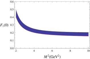
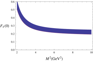
Figure 1: Dependence of $F_{1}^{B_{s}\to f_{0}}(0)$ and $F_{T}^{B_{s}\to f_{0}}(0)$ on the Borel parameter $M^{2}$.

To describe the form factors in the whole kinematically accessible $q^{2}$ region, we use the parameterization ${F_{i}(q^{2})=\frac{F_{i}(0)}{1-a_{i}q^{2}/m_{B_{s}}^{2}+b_{i}(q^{2}/m_{B_{s}}^{2})^{2}}}$, $i\in\{1,0,T\}$; the parameters $F_{i}(0)$, $a_{i}$ and $b_{i}$ are obtained through fitting the form factors computed numerically in the large recoil region. Our results are collected in Table 1, where uncertainties in the results are due to the input parameters, $s_{0}$ and $M^{2}$.

Table 1: $B_{s}\to f_{0}$ form factors in the LCSR.

	$F_{i}(q^{2}=0)$	$a_{i}$	$b_{i}$
$F_{1}$	$0.185\pm 0.029$	$1.44^{+0.13}_{-0.09}$	$0.59^{+0.07}_{-0.05}$
$F_{0}$	$0.185\pm 0.029$	$0.47^{+0.12}_{-0.09}$	$0.01^{+0.08}_{-0.09}$
$F_{T}$	$0.228\pm 0.036$	$1.42^{+0.13}_{-0.10}$	$0.60^{+0.06}_{-0.05}$

3 $B_{s}\to M_{c{\bar{c}}}L$ decays

The effective hamiltonian responsible for decays induced by the $b\to c{\bar{c}}s$ transition is:

$${\cal H}_{\rm eff} = \frac{G_{F}}{\sqrt{2}}\big{\{}V_{cb}V_{cs}^{*}\big{[}C_{1}({\mu})O_{1}+C_{2}({\mu})O_{2}\big{]}-V_{tb}V_{ts}^{*}\big{[}{\sum\limits_{i=3}^{10,7\gamma,8g}}C_{i}({\mu})O_{i}({\mu})\big{]}\big{\}},$$ (6)

where $G_{F}$ is the Fermi constant, $O_{i}$ are the four-quark or magnetic-moment operators and $C_{i}$ are Wilson coefficients. With the assumption of the CKM unitarity and the neglect of the tiny $V_{ub}V_{us}^{*}$, we have $V_{tb}V_{ts}^{*}=-V_{cb}V_{cs}^{*}$.

The simplest approach to compute the matrix element of the effective four-quark or magnetic-moment operators is the naive factorization approach. In this approach neglecting the magnetic moment operators whose contributions are suppressed by $\alpha_{s}$, the $B_{a}\to M_{c{\bar{c}}}L$ amplitude reads (($a$ being a light flavour index))

$${\cal A}(B_{a}\to M_{c{\bar{c}}}L)={G_{F}\over\sqrt{2}}V_{cb}V_{cs}^{*}a_{2}^{\rm eff}(\mu)\langle{M_{c{\bar{c}}}}|{\bar{c}}\gamma^{\mu}(1-\gamma_{5})c\,|{0}\rangle\langle{L}|{\bar{s}}\gamma_{\mu}(1-\gamma_{5})b|\bar{B}_{a}\rangle\,,$$ (7)

where $a_{2}^{\rm eff}(\mu)$ is a combination of the Wilson coefficients: $a_{2}^{\rm eff}(\mu)=a_{2}(\mu)+a_{3}(\mu)+a_{5}(\mu)$ and and $a_{2}=C_{2}+{C_{1}/N_{c}}$, $a_{3}=C_{3}+{C_{4}/N_{c}}+{3\over 2}e_{c}\left(C_{9}+{C_{10}/N_{c}}\right)$ and $a_{5}=C_{5}+{C_{6}/N_{c}}+{3\over 2}e_{c}\left(C_{7}+{C_{8}/N_{c}}\right)$ with $e_{c}=2/3$ and $N_{c}=3$. This factorization approach allows us to express the decay amplitudes in terms of the heavy-to-light form factors and the decay constant of the emitted meson. Unfortunately, one severe drawback is that naive factorization badly reproduces several branching ratios for which experimental data are available. In particular, the $b\to c{\bar{c}}s$ induced modes under scrutiny are color suppressed, and the predictions of naive factorization will typically undershoot the data. The most striking discrepancy is for the $B_{d}$ decay modes with $\chi_{c0}$ in the final state, which have a sizeable rate but their decay amplitude vanishes in the factorization approach Colangelo:2002mj .

Several modifications to the naive factorization ansatz have been proposed and in particular in this work we will explore one possibility by treating the Wilson coefficients as effective parameters to be determined from experiment. In principle, it implies that such coefficients are channel dependent. However for channels related by invoking flavour symmetries, universal values for the coefficients can be assumed. In our case, this generalized factorization approach consists in considering the quantity $a_{2}^{\rm eff}$ in (7) as a process dependent parameter to be fixed from experiment. In particular, if one assumes the flavor $SU(3)$ symmetry, $B$ ($B_{u}$ or $B_{d}$) decays can be related to analogous $B_{s}$ decays, so that experimental data on $B$ decays provide a prediction for $B_{s}$ related ones.

Our strategy is to exploit the existing experimental data for $B$ decay modes to determine an effective parameter $a_{2}^{\rm eff}$ and, assuming $SU(3)_{F}$ symmetry, to use these values to predict the flavour related $B_{s}$ decays. In the case of modes with $\chi_{c1}$ in the final state, we will determine the combination $f_{\chi_{c1}}a_{2}^{\rm eff}$ since sizable uncertainties may be introduced to the Wilson coefficient but will cancel in the predictions of branching ratios. In this procedure, we use two sets of form factors: the one obtained using sum rules based on the short-distance expansion Colangelo:1995jv , and the set in Ball:2004ye based on the light-cone expansion. In the case of $B_{s}\to\phi$ and $B_{s}\to f_{0}(980)$ we use form factors determined by LCSR Ball:2004ye ; Colangelo:2010bg . $B_{s}\to\eta^{(\prime)}$ form factors are related to the analogous $B\to K$ form factors and the mixing angle between $\eta$ and $\eta^{\prime}$ in the flavor basis Feldmann:1998vh can be fixed to the value measured by the KLOE Collaboration: $\theta=\big{(}41.5\pm 0.3_{stat}\pm 0.7_{syst}\pm 0.6_{th}\big{)}^{\circ}$ kloe , which is also supported by a QCD sum rule analysis of the radiative $\phi\to\eta^{(\prime)}\gamma$ modes DeFazio:2000my . The Wilson coefficients for $B_{s}\to M_{c{\bar{c}}}f_{0}(980)$ are obtained using the effective value determined from $B\to M_{c{\bar{c}}}K$. Most of other numerical inputs are taken from the particle data group and we refer to Ref. Colangelo:2010zz for more details.

The predictions for branching ratios of $B_{s}$ decays are given in Tables 2 and 3. In Table 2 the available experimental data Amsler:2008zzb ; :2009usa ; talkbelle are also reported, with a satisfactory agreement with the predictions. In theoretical predictions we have included the uncertainty on the form factors at $q^{2}=0$ and on the experimental branching ratios, but in the case of the modes involving $\eta$ or $\eta^{\prime}$ the uncertainty on the form factors is not included since the dependence on the form factors will cancel when the branching ratios of $B\to J/\psi K$ decays are related to the corresponding $B_{s}$ decays.

Table 2: Branching ratios (in units of $10^{-4}$) of $B_{s}\to M_{c\bar{c}}\,L$ using the form factors in Colangelo:1995jv (CDSS) and in Ball:2004ye (BZ). Experimental results are taken from PDG Amsler:2008zzb , except for $B_{s}\to J/\psi\,\eta\,(\eta^{\prime})$ measured by Belle Collaboration :2009usa and the bound for $B_{s}\to J/\psi\,f_{0}$ is from Ref. talkbelle .

mode	${\cal B}$ (CDSS)	${\cal B}$ (BZ)	Exp.	mode	${\cal B}$ (CDSS)	${\cal B}$ (BZ)
$J/\psi\,\eta$	$4.3\pm 0.2$	$4.2\pm 0.2$	$3.32\pm 1.02$	$\eta_{c}\,\eta$	$4.0\pm 0.7$	$3.9\pm 0.6$
$J/\psi\,\eta^{\prime}$	$4.4\pm 0.2$	$4.3\pm 0.2$	$3.1\pm 1.39$	$\eta_{c}\,\eta^{\prime}$	$4.6\pm 0.8$	$4.5\pm 0.7$
$\psi(2S)\,\eta$	$2.9\pm 0.2$	$3.0\pm 0.2$		$\eta_{c}(2S)\,\eta$	$1.5\pm 0.8$	$1.4\pm 0.7$
$\psi(2S)\,\eta^{\prime}$	$2.4\pm 0.2$	$2.5\pm 0.2$		$\eta_{c}(2S)\,\eta^{\prime}$	$1.6\pm 0.9$	$1.5\pm 0.8$
$J/\psi\,\phi$	—	$16.7\pm 5.7$	$13\pm 4$	$\eta_{c}\,\phi$	—	$15.0\pm 7.8$
$\psi(2S)\,\phi$	—	$8.3\pm 2.7$	$6.8\pm 3.0$
$\chi_{c1}\,\eta$	$2.0\pm 0.2$	$2.0\pm 0.2$		$\chi_{c1}\,f_{0}$	$1.88\pm 0.77$	$0.73\pm 0.30$
$\chi_{c1}\,\eta^{\prime}$	$1.9\pm 0.2$	$1.8\pm 0.2$		$\chi_{c1}\,\phi$	—	$3.3\pm 1.3$
$J/\psi\,f_{0}$	$4.7\pm 1.9$	$2.0\pm 0.8$	$<3.26$	$\eta_{c}\,f_{0}$	$4.1\pm 1.7$	$2.0\pm 0.9$
$\psi(2S)\,f_{0}$	$2.3\pm 0.9$	$0.89\pm 0.36$		$\eta_{c}(2S)\,f_{0}$	$0.58\pm 0.38$	$1.3\pm 0.8$

As appears from Tables 2 and 3 all the considered modes have sizable branching fractions which are large enough to make them promising candidates for the measurement of $\beta_{s}$. The modes involving $\eta,\,\eta^{\prime},\,f_{0}$ present, with respect to the golden mode $B_{s}\to J/\psi\phi$, the advantage that the final state is a CP eigenstate, not requiring angular analysis. However, channels with $\eta$ and $\eta^{\prime}$ can be useful only after a number of events have been accumulated, since at least two photons are required for the reconstruction.

Table 3: Branching ratios of $B_{s}$ decays into p-wave charmonia (unit: $10^{-4}$).

mode	${\cal B}$	mode	${\cal B}$	mode	${\cal B}$
$\chi_{c0}\,\eta$	$0.85\pm 0.13$	$\chi_{c2}\,\eta$	$<0.17$	$h_{c}\,\eta$	$<0.23$
$\chi_{c0}\,\eta^{\prime}$	$0.87\pm 0.13$	$\chi_{c2}\,\eta^{\prime}$	$<0.17$	$h_{c}\,\eta^{\prime}$	$<0.23$
$\chi_{c0}\,f_{0}$	$1.15\pm 0.17$	$\chi_{c2}\,f_{0}$	$<0.29$	$h_{c}\,f_{0}$	$<0.30$
$\chi_{c0}\,\phi$	$1.59\pm 0.38$	$\chi_{c2}\,\phi$	$<0.10(0.62\pm 0.17)$	$h_{c}\,\phi$	$(<1.9)$

As discussed in Stone:2008ak ; Colangelo:2010bg ; Leitner:2010fq , $B_{s}\to J/\psi f_{0}$ has appealing features since, compared with the $\eta^{(^{\prime})}$, the $f_{0}$ can be easily identified in the $\pi^{+}\pi^{-}$ final state with a large BR: ${\cal B}(f_{0}\to\pi^{+}\pi^{-})=(50^{+7}_{-8})\%$ Ablikim:2004cg , so that this channel can likely be accessed. At present, the Belle Collaboration has recently provided the following upper limit talkbelle :

$${\cal B}(B_{s}\to J/\psi f_{0})\times{\cal B}(f_{0}\to\pi^{+}\pi^{-})<1.63\times 10^{-4}\,$$ (8)

marginally in accordance with our prediction.

Let us come to $B_{s}$ decays to $p$-wave charmonia. Among these decays, the only one with non vanishing amplitude in the factorization assumption is that with $\chi_{c1}$ in the final state. In the other cases, i.e. modes involving $\chi_{c0,2}$ or $h_{c}$, which we show in Table 3, results are obtained determining the decay amplitudes from the $B$ decay data by making use of the SU(3) symmetry. In this case, the differences between the $B$ and $B_{s}$ decays arise from the phase space and lifetimes of the heavy mesons. As for the mechanism inducing such processes, one possibility is that rescattering may be responsible of their observed branching fractions, as proposed in Ref.Colangelo:2002mj . Among these channels, $B_{s}\to\chi_{c0}\phi$ is of prime interest and promising for both hadron colliders and $B$ factories.

4 conclusion

Recent results in the $B_{s}$ sector strongly require theoretical efforts to shed light on which are the most promising decay modes to unreveal new physics. In this work we have analyzed channels induced by the $b\to c{\bar{c}}s$ transition. Modes with a charmonium state plus $\eta$, $\eta^{\prime}$, $f_{0}(980)$ are the most promising, being CP eigenstates not requiring an angular analysis. In particular, the case of $f_{0}$ is particularly suitable in view of its easier reconstruction in the subsequent decay to $\pi^{+}\pi^{-}$. As a preliminary step we have used the light-cone sum rules to compute the $B_{s}\to f_{0}(980)$ form factors which are necessary inputs in the analysis of $B_{s}$ decays.

References

- (1) V. M. Abazov et al. [D0 Collaboration], Phys. Rev. D 76, 057101 (2007); Phys. Rev. Lett. 101, 241801 (2008); T. Aaltonen et al. [CDF collaboration], Phys. Rev. Lett. 100, 121803 (2008); Phys. Rev. Lett. 100 161802 (2008).
- (2) E. Barberio et al. [Heavy Flavor Averaging Group], arXiv:0808.1297 [hep-ex].
- (3) L. Oakes for the CDF Collaboration, Talk at FPCP 2010, Torino.
- (4) P. Colangelo, F. De Fazio and W. Wang, Phys. Rev. D 81, 074001 (2010).
- (5) P. Colangelo, F. De Fazio and W. Wang, arXiv:1009.4612 [hep-ph].
- (6) P. Colangelo and A. Khodjamirian, in ”At the Frontier of Particle Physics/Handbook of QCD”, ed. by M. Shifman (World Scientific, Singapore, 2001), vol. 3, pages 1495-1576, arXiv:hep-ph/0010175.
- (7) P. Colangelo et al. Phys. Lett. B 542 (2002) 71; Phys. Rev. D 69 (2004) 054023.
- (8) C. Amsler et al. [Particle Data Group], Phys. Lett. B 667, 1 (2008).
- (9) P. Colangelo, et al. Phys. Rev. D 53, 3672 (1996) [Erratum-ibid. D 57, 3186 (1998)].
- (10) P. Ball and R. Zwicky, Phys. Rev. D 71, 014015 (2005); Phys. Rev. D 71, 014029 (2005).
- (11) T. Feldmann, P. Kroll and B. Stech, Phys. Rev. D 58, 114006 (1998); Phys. Lett. B 449, 339 (1999); T. Feldmann, Int. J. Mod. Phys. A 15, 159 (2000).
- (12) F. Ambrosino et al. [KLOE Collaboration], Phys. Lett. B 648, 267 (2007).
- (13) F. De Fazio and M. R. Pennington, JHEP 0007 (2000) 051.
- (14) I. Adachi et al. [Belle Collaboration], arXiv:0912.1434.
- (15) R. Louvot [Belle Collaboration], arXiv:1009.2605 [hep-ex].
- (16) S. Stone and L. Zhang, Phys. Rev. D 79 (2009) 074024; arXiv:0909.5442.
- (17) O. Leitner et al., arXiv:1003.5980 [hep-ph].
- (18) M. Ablikim et al. [BES Collaboration], Phys. Rev. D 70, 092002 (2004); ibid: D 72, 092002 (2005).