Analysis of an interface stabilised finite element method: The advection-diffusion-reaction equation

Abstract

Analysis of an interface stabilised finite element method for the scalar advection-diffusion-reaction equation is presented. The method inherits attractive properties of both continuous and discontinuous Galerkin methods, namely the same number of global degrees of freedom as a continuous Galerkin method on a given mesh and the stability properties of discontinuous Galerkin methods for advection dominated problems. Simulations using the approach in other works demonstrated good stability properties with minimal numerical dissipation, and standard convergence rates for the lowest order elements were observed. In this work, stability of the formulation, in the form of an inf-sup condition for the hyperbolic limit and coercivity for the elliptic case, is proved, as is order $k+1/2$ order convergence for the advection-dominated case and order $k+1$ convergence for the diffusive limit in the $L^{2}$ norm. The analysis results are supported by a number of numerical experiments.

1 Introduction

Discontinuous Galerkin methods have proven effective and popular for classes of partial differential equations, in particular transport equations in which advection is dominant. The attractive stability properties of suitably constructed discontinuous Galerkin methods and the possibility of matching non-conforming meshes are advantageous, but do come at the cost of an increased number of global degrees of freedom on a given mesh compared to continuous Galerkin methods. In a number of recent works, advances have been made in reconciling the appealing features of continuous and discontinuous Galerkin methods in one framework. Works in this direction include those of Hughes et al. [1], Labeur and Wells [2] and Cockburn et al. [3] for the advection-diffusion equation, Burman and Stamm [4] for advection-reaction equation, and Labeur and Wells [2] and Labeur and Wells [5] for the incompressible Navier-Stokes equations. These methods generally strive for a reduction in the number of global degrees of freedom relative to a conventional discontinuous Galerkin method without sacrificing other desirable features. In this work, stability and convergence estimates are presented for one such method applied to the scalar advection-diffusion-reaction equation, namely the interface stabilised method as formulated in Labeur and Wells [2].

The principle behind the interface stabilised method is simple: the equation of interest is posed cell-wise subject to weakly imposed Dirichlet boundary conditions in the spirit of discontinuous Galerkin methods. The boundary condition which is weakly satisfied is provided by an ‘interface’ function that lives only on cell facets and is single-valued on cell facets. An equation for this additional field is furnished by insisting upon weak continuity of the so-called ‘numerical flux’ across cell facets. This weak continuity of the numerical flux is in contrast with typical discontinuous Galerkin methods which satisfy continuity of the numerical flux across cell facets point-wise by construction. For particular choices in the method, it may be possible to achieve point-wise continuity. Upwinding of the advective flux at interfaces can be incorporated naturally in the definition of the numerical flux, as is typical for discontinuous Galerkin methods. By building a degree of continuity into the interface function spaces (at cell vertices in two dimensions and across cell edges in three dimensions), the number of global degrees of freedom is equal to that for a continuous Galerkin method on the same mesh. The key to this reduction in the number of global degrees of freedom is that functions which are defined on cells are not linked directly across cell facets, rather they communicate only via the interface function. Therefore, functions on cells can be eliminated locally (cell-wise) in favour of the functions that live on cell facets. Outwardly the approach appears to have elements in common with mortar methods, and could serve to elucidate links between mortar and discontinuous Galerkin methods.

The motivation for analysing the interface stabilised method comes from the observed performance of the method for the advection-diffusion in Hughes et al. [1] and Labeur and Wells [2] and for the incompressible Navier-Stokes equations in Labeur and Wells [2], and for the Navier-Stokes equations on moving domains, as presented in Labeur and Wells [5]. The method was observed in simulations to be robust and only minimal numerical dissipation could be detected. Labeur and Wells [2] also showed that the methodology can lead to a stable formulation for Stokes equation using equal-order Lagrange basis functions for the velocity and the pressure. The method examined in this work is closely related to that formulated by Hughes et al. [1] for the advection-diffusion equation, and analysed in Buffa et al. [6]. Buffa et al. [6] proved stability for a streamline-diffusion stabilised variant of the method, but not for the original formulation. For the case without the additional streamline diffusion term, stability was demonstrated for some computed examples by evaluating the inf-sup condition numerically. However, in the absence of an analytical stability estimate convergence estimates could not be formulated. The stability and error estimates developed here for a method without an additional streamline diffusion term are made possible by: (1) the different and transparent format in which the problem is posed; and (2) the different machinery that is brought to bear on the problem. With respect to the last point, advantage is taken of some developments formulated by Ern and Guermond [7].

In the remainder of this work, the equation of interest and the numerical method to be analysed are first formalised. This is followed by analysis of the hyperbolic case, for which satisfaction of an inf-sup is demonstrated. The the diffusive limit case is then considered, for which demonstration of coercivity suffices. The results of some numerical simulations are then presented in support of the analysis, after which conclusions are drawn.

2 Interface stabilised method

2.1 Model problem

Consider a polygonal domain $\Omega\subset\mathbb{R}^{d}$, where $1\leq d\leq 3$, with boundary $\Gamma=\partial\Omega$. The unit outward normal vector to the domain is denoted by $\boldsymbol{n}$. The advection-diffusion-reaction equation reads:

$$\mu u+\boldsymbol{a}\cdot\nabla u-\kappa\nabla^{2}u=f\quad{\rm in}\ \Omega,$$ (1)

where $\mu\geq 0$ and $\kappa\geq 0$ are assumed to be constant, $\boldsymbol{a}:\Omega\rightarrow\mathbb{R}^{d}$ is a divergence-free vector field that is Lipschitz continuous on $\bar{\Omega}$ and satisfies $\left\|{\boldsymbol{a}}\right\|_{L^{\infty}(\Omega)}\leq 1$, and $f:\Omega\rightarrow\mathbb{R}$ is a suitably regular source term. The divergence-free condition on $\boldsymbol{a}$ can easily be relaxed to $\mu-(1/2)\nabla\cdot\boldsymbol{a}>0$. Portions of the boundary on which $\boldsymbol{a}\cdot\boldsymbol{n}\geq 0$ are denoted by $\Gamma_{+}$, and portions on which $\boldsymbol{a}\cdot\boldsymbol{n}<0$ are denoted by $\Gamma_{-}$. A function $\zeta$ is defined on boundaries such that $\zeta=0$ on outflow portions of the boundary ($\Gamma_{+}$) and $\zeta=1$ on inflow portions of the boundary ($\Gamma_{-}$).

For the case $\kappa>0$, the boundary is partitioned into $\Gamma_{N}$ and $\Gamma_{D}$ such that $\overline{\Gamma_{N}\cup\Gamma_{D}}=\Gamma$ and $\Gamma_{N}\cap\Gamma_{D}=\emptyset$, and the boundary conditions

$$\begin{split}\left({-\zeta u\boldsymbol{a}+\kappa\nabla u}\right)\cdot\boldsymbol{n}&=g\quad{\rm on}\ \Gamma_{N},\\ u&=0\quad{\rm on}\ \Gamma_{D},\end{split}$$ (2)

are considered, where $g:\Gamma_{N}\rightarrow\mathbb{R}$ is a suitably smooth prescribed function. For the case $\kappa=0$, then $\Gamma_{D}=\emptyset$, $\Gamma_{N}=\Gamma_{-}$ and the considered boundary condition reads:

$$-u\boldsymbol{a}\cdot\boldsymbol{n}=g\quad{\rm on}\ \Gamma_{-}.$$ (3)

2.2 The method

Let $\mathcal{T}$ be a triangulation of $\Omega$ into non-overlapping simplices such that $\mathcal{T}=\left\{{K}\right\}$. A simplex $K\in\mathcal{T}$ will be referred to as a cell and a measure of the size of a cell $K$ will be denoted by $h_{K}$, with the usual assumption that $h_{K}\leq 1$, and $h=\max_{K\in\mathcal{T}}h_{K}$. The boundary of a cell $K$ is denoted by $\partial K$ and the outward unit normal to a cell is denoted by $\boldsymbol{n}$. The outflow portion of a cell boundary is the portion on which $\boldsymbol{a}\cdot\boldsymbol{n}\geq 0$, and is denoted by $\partial K_{+}$. The inflow portion of a cell boundary is the portion on which $\boldsymbol{a}\cdot\boldsymbol{n}<0$, and is denoted by $\partial K_{-}$. As for the exterior boundary, the function $\zeta$ is defined such that $\zeta=0$ on $\partial K_{+}$ and $\zeta=1$ on $\partial K_{-}$. The set of all facets $\mathcal{F}=\left\{{F}\right\}$ contained in the mesh will be used, as will the union of all facets, which is denoted by $\Gamma^{0}$. Adjacent cells are considered to share a common facet $F$.

The bilinear and linear forms for the advection-diffusion-reaction equation are now introduced. Using the notation $\boldsymbol{w}=\left({w,\bar{w}}\right)$ and $\boldsymbol{v}=\left({v,\bar{v}}\right)$, consider the bilinear form:

$$B\left({\boldsymbol{w},\boldsymbol{v}}\right)=\int_{\Omega}\mu wv\,dx+\int_{\Omega}\left({-\boldsymbol{a}w+\kappa\nabla w}\right)\cdot\nabla v\,dx\\ +\sum_{K}\int_{\partial K}\left({-\boldsymbol{a}w+\kappa\nabla w-\left({\zeta\boldsymbol{a}-\frac{\alpha\kappa}{h_{K}}\boldsymbol{n}}\right)\left({\bar{w}-w}\right)}\right)\cdot\boldsymbol{n}\left({\bar{v}-v}\right)\,ds\\ +\sum_{K}\int_{\partial K}\kappa\left({\bar{w}-w}\right)\nabla v\cdot\boldsymbol{n}\,ds+\int_{\Gamma_{+}}\boldsymbol{a}\cdot\boldsymbol{n}\bar{v}\bar{w}\,ds$$ (4)

and the linear form

$$L\left({\boldsymbol{v}}\right)=\int_{\Omega}fv\,dx+\int_{\Gamma_{N}}g\bar{v}\,ds,$$ (5)

where $\alpha\geq 0$. The relevant finite element function spaces for the problem which will be considered read

$$W_{h} =\left\{{w_{h}\in L^{2}\left({\Omega}\right),w_{h}|_{K}\in P_{k}\left({K}\right)\forall K\in\mathcal{T}}\right\},$$ (6)

$$\bar{W}_{h} =\left\{{\bar{w}_{h}\in H^{l}\left({\Gamma^{0}}\right),\bar{w}_{h}|_{F}\in P_{k}\left({F}\right)\forall F\in\mathcal{F},\bar{w}_{h}=0\ {\rm on}\ \Gamma_{D}}\right\},$$ (7)

where $0\leq l\leq 1$ and $P_{k}(K)$ denotes the space of standard Lagrange polynomial functions of order $k$ on cell $K$. The space $W_{h}$ is the usual space commonly associated with discontinuous Galerkin methods, and the space $\bar{W}_{h}$ contains Lagrange polynomial shape functions that ‘live’ only on cell facets and are single-valued on facets. The choice of $l$, which determines the regularity of the facet functions at cell vertices in two dimensions and across cell edges in three dimensions, will have a significant impact on the structure of the resulting matrix problem. Using the notation $W^{\star}_{h}=W_{h}\times\bar{W}_{h}$ and $\boldsymbol{v}_{h}=\left({v_{h},\bar{v}_{h}}\right)$, the finite element problem of interest reads: find $\boldsymbol{u}_{h}\in W_{h}^{\star}$ such that

$$B\left({\boldsymbol{u}_{h},\boldsymbol{v}_{h}}\right)=L\left({\boldsymbol{v}_{h}}\right)\quad\forall\boldsymbol{v}_{h}\in W^{\star}_{h}.$$ (8)

To motivate the terms appearing in the bilinear form, it is useful to consider the case in which $v=0$ and the case in which $\bar{v}=0$ separately. Considering first $\boldsymbol{v}_{h}=\left({v_{h},0}\right)$, the variational problem corresponding to equation (8) for a single cell reads: given $\bar{u}_{h}\in\bar{W}_{h}$, find $u_{h}\in W_{h}$ such that for all $v_{h}\in W_{h}$

$$\int_{K}\mu u_{h}v_{h}\,dx+\int_{K}\boldsymbol{\sigma}\left({u_{h}}\right)\cdot\nabla v_{h}\,dx-\int_{\partial K}\bar{\boldsymbol{\sigma}}\left({\boldsymbol{u}_{h}}\right)\cdot\boldsymbol{n}v_{h}\,ds\\ +\int_{\partial K}\kappa\left({\bar{u}_{h}-u_{h}}\right)\nabla v_{h}\cdot\boldsymbol{n}\,ds=\int_{K}fv_{h}\,dx,$$ (9)

where $\boldsymbol{\sigma}\left({w}\right)=-\boldsymbol{a}\nabla w+\kappa\nabla w$ is the usual flux vector and $\bar{\boldsymbol{\sigma}}\left({\boldsymbol{w}}\right)$ is a ‘numerical flux’,

$$\bar{\boldsymbol{\sigma}}\left({\boldsymbol{w}}\right)=-\boldsymbol{a}w+\kappa\nabla w-\left({\zeta\boldsymbol{a}-\frac{\alpha\kappa}{h_{K}}\boldsymbol{n}}\right)\left({\bar{w}-w}\right).$$ (10)

The problem in equation (9) is essentially a cell-wise postulation of a Galerkin problem for equation (1) subject to the weak satisfaction of the boundary condition $u_{h}=\bar{u}_{h}$. In the numerical flux, the presence of the term $\zeta$ provides for upwinding of the advective part of the flux, and the term $\left({\alpha\kappa/{h_{K}}}\right)\boldsymbol{n}\left({\bar{w}-w}\right)$ is an interior penalty-type contribution to the numerical flux [8]. The term $\int_{\partial K}\kappa\left({\bar{u}_{h}-u_{h}}\right)\nabla v_{h}\cdot\boldsymbol{n}\,ds$ is typical of discontinuous Galerkin methods for elliptic problems, and resembles that in Arnold et al. [8] for the Poisson equation. The numerical flux can be evaluated on both sides of a facet. On the outflow (upwind) portion of a cell boundary, the advective part of the numerical flux is equal to the regular advective flux. On the inflow (downwind) portion of a cell boundary, the advective part of the numerical flux depends on the interface function, taking on $-\boldsymbol{a}\bar{u}$. The diffusive numerical flux on a cell boundary has contributions from the regular flux and a penalty-like contribution which depends on the difference between $w_{h}$ and the interface function $\bar{w}_{h}$. Setting $v_{h}=1$ in equation (9),

$$\int_{K}\mu u_{h}\,dx-\int_{\partial K}\bar{\boldsymbol{\sigma}}\left({\boldsymbol{u}_{h}}\right)\cdot\boldsymbol{n}\,ds=\int_{K}f\,dx,$$ (11)

which demonstrates local conservation in terms of the numerical flux. Note that the numerical flux defined in equation (10) is not single-valued on cell facets. Setting $\boldsymbol{v}_{h}=\left({0,\bar{v}_{h}}\right)$ furnishes the problem: given $u_{h}\in W_{h}$, find $\bar{u}_{h}\in\bar{W}_{h}$ such that for all $\bar{v}_{h}\in\bar{W}_{h}$

$$\sum_{K}\int_{\partial K}\bar{\boldsymbol{\sigma}}\left({\boldsymbol{u}_{h}}\right)\cdot\boldsymbol{n}\bar{v}_{h}\,ds+\int_{\Gamma_{+}}\boldsymbol{a}\cdot\boldsymbol{n}\bar{u}_{h}\bar{v}_{h}\,ds=\int_{\Gamma_{N}}g\bar{v}_{h}\,ds,$$ (12)

which is a statement of weak continuity of the numerical flux across cell facets.

Noteworthy in the bilinear form is that the functions $w_{h}$, which are discontinuous across cell facets, are not linked directly across facets. They are only linked implicitly through their interaction with $\bar{w}_{h}$. Setting $\boldsymbol{v}_{h}=\left({v_{h},0}\right)$ leads to a local (cell-wise) problem, which, given $\bar{u}_{h}$ and $f$ can be solved locally to eliminate $u_{h}$ in favour of $\bar{u}_{h}$. This process is commonly referred to as static condensation. Then, setting $\boldsymbol{v}_{h}=\left({0,\bar{v}_{h}}\right)$, one can solve a global problem to yield the interface solution $\bar{u}_{h}$. The field $u_{h}$ can then be recovered trivially element-wise. To formulate a global problem with the same number of degrees as a continuous finite element method, $l$ in equation (7) must be chosen such that there is only one degree of freedom at a given point; the interface functions are continuous at cell vertices in two dimensions and along cell edges in three dimensions. Further details on the formulation of the interface stabilised method and various algorithmic details can be found in Labeur and Wells [2].

The formulation of Hughes et al. [1] can be manipulated into framework presented in this section, and in the hyperbolic limit coincides with the formulation presented here. In the case of diffusion, Hughes et al. [1] adopted an upwinded diffusive flux whereas the diffusive flux is centred in the present method. The formulation presented in Cockburn et al. [3] follows the same framework as Labeur and Wells [2], although the use of functions lying in $L^{2}\left({\Gamma^{0}}\right)$ on facets is advocated.

The method is now shown to be consistent with equation (1). If $u$ solves equation (1), it is chosen to define $\boldsymbol{u}=\left({u,u}\right)$. The action of the trace operator in the second slot is implicit in this definition (this will be expanded upon in Section 3). With this definition of $\boldsymbol{u}$ consistency can be addressed.

Lemma 1 (consistency).

If $\boldsymbol{u}=\left({u,u}\right)$, where $u\in H^{m}\left({\Omega}\right)$ is a solution to (1) with $m=2$ if $\kappa>0$ and $m=1$ otherwise, and if $\boldsymbol{u}_{h}$ solves (8), then for all $\boldsymbol{v}_{h}\in W_{h}^{\star}$

$$B\left({\boldsymbol{u}-\boldsymbol{u}_{h},\boldsymbol{v}_{h}}\right)=0.$$ (13)

Proof.

Since $\boldsymbol{u}_{h}$ is a solution to (8) and due to the bilinear nature of $B$, it suffices to demonstrate that $B\left({\boldsymbol{u},\boldsymbol{v}_{h}}\right)-L\left({\boldsymbol{v}_{h}}\right)=0$. Considering first $B\left({\boldsymbol{u},\left({v_{h},0}\right)}\right)-L\left({\left({v_{h},0}\right)}\right)$, which is presented in equation (9), after applying integration by parts

$$B\left({\boldsymbol{u},\left({v_{h},0}\right)}\right)-L\left({\left({v_{h},0}\right)}\right)=\int_{K}\left({\mu u+\boldsymbol{a}\nabla u-\kappa\nabla^{2}u-f}\right)v_{h}\,dx=0,$$ (14)

since $u$ satisfies (1) for $\kappa=0$. Considering now $B\left({\boldsymbol{u},\left({0,\bar{v}_{h}}\right)}\right)-L\left({\left({0,\bar{v}_{h}}\right)}\right)$, which is presented in equation (12),

$$B\left({\boldsymbol{u},\left({0,\bar{v}_{h}}\right)}\right)-L\left({\left({0,\bar{v}_{h}}\right)}\right)=\int_{\Gamma_{N}}\left({\left({-\zeta u\boldsymbol{a}+\kappa\nabla u}\right)\cdot\boldsymbol{n}-g}\right)\bar{v}_{h}\,ds=0,$$ (15)

since $u$ satisfies the boundary condition in (3). Summing equations (14) and (14) and subtracting $B\left({\boldsymbol{u}_{h},\boldsymbol{v}_{h}}\right)-L\left({\boldsymbol{v}_{h}}\right)=0$ concludes the proof. ∎

2.3 Limit cases

The method will be analysed for the hyperbolic ($\kappa=0$) and elliptic ($\boldsymbol{a}=\boldsymbol{0},\mu=0$) limit cases. The bilinear form is therefore decomposed into advective and diffusive parts,

$$B\left({\boldsymbol{w},\boldsymbol{v}}\right)=B_{A}\left({\boldsymbol{w},\boldsymbol{v}}\right)+B_{D}\left({\boldsymbol{w},\boldsymbol{v}}\right),$$ (16)

where

$$B_{A}\left({\boldsymbol{w},\boldsymbol{v}}\right)=\int_{\Omega}\mu wv\,dx-\sum_{K}\int_{K}\boldsymbol{a}w\cdot\nabla v\,dx-\sum_{K}\int_{\partial K_{+}}\boldsymbol{a}\cdot\boldsymbol{n}w\left({\bar{v}-v}\right)\,ds\\ -\sum_{K}\int_{\partial K_{-}}\boldsymbol{a}\cdot\boldsymbol{n}\bar{w}\left({\bar{v}-v}\right)\,ds+\int_{\Gamma_{+}}\boldsymbol{a}\cdot\boldsymbol{n}\bar{w}\bar{v}\,ds$$ (17)

and

$$B_{D}\left({\boldsymbol{w},\boldsymbol{v}}\right)=\sum_{K}\int_{K}\kappa\nabla w\cdot\nabla v\,dx\\ +\sum_{K}\int_{\partial K}\left({\kappa\nabla w+\frac{\alpha\kappa}{h_{K}}\boldsymbol{n}\left({\bar{w}-w}\right)}\right)\cdot\boldsymbol{n}\left({\bar{v}-v}\right)\,ds\\ +\sum_{K}\int_{\partial K}\kappa\left({\bar{w}-w}\right)\nabla v\cdot\boldsymbol{n}\,ds.$$ (18)

Stability and error estimates will be proved by analysing $B_{A}\left({\boldsymbol{w},\boldsymbol{v}}\right)$ and $B_{D}\left({\boldsymbol{w},\boldsymbol{v}}\right)$ independently.

2.4 Conventional discontinuous Galerkin methods as a special case

If the functions defined on facets are defined to be in $L^{2}\left({\Gamma^{0}}\right)$ ($l=0$ in equation (7)), then for the hyperbolic case the formulation reduces to the conventional discontinuous Galerkin formulation with full upwinding of the advective flux [9, 10, 11]. In the diffusive limit, it reduces to a method which closely resembles the symmetric interior penalty method [12, 13]. Of prime practical interest is the case where the interface functions are continuous as this leads to the fewest number of global degrees of freedom, but the special case of $l=0$ is considered briefly in this section to illustrate a link with conventional discontinuous Galerkin methods.

For the case $\mu=\kappa=0$, setting $v_{h}=0$ everywhere and $\bar{v}_{h}=0$ everywhere with the exception of one interior facet $F$, the method implies that at the facet $F$

$$\int_{F}\boldsymbol{a}\bar{w}_{h}\cdot\boldsymbol{n}_{+}\bar{v}_{h}\,ds=\int_{F_{-}}\boldsymbol{a}w_{h+}\cdot\boldsymbol{n}_{+}\bar{v}_{h}\,ds,$$ (19)

where the subscript ‘$+$’ indicates functions evaluated on the boundary of the upwind cell. This implies that for a given $w_{h}$, the facet function $\bar{w}_{h}$ simply takes on the upwind value on each facet. Inserting this into equation (17) and setting $\bar{v}_{h}=0$,

$$B_{A}\left({w_{h},v_{h}}\right)=\int_{\Omega}\mu w_{h}v_{h}\,dx-\sum_{K}\int_{K}\boldsymbol{a}w_{h}\cdot\nabla v_{h}\,dx\\ +\sum_{K}\int_{\partial K_{+}}\boldsymbol{a}\cdot\boldsymbol{n}w_{h}v_{h}\,ds+\sum_{K}\int_{\partial K_{-}}\boldsymbol{a}\cdot\boldsymbol{n}w_{h+}v_{h}\,ds,$$ (20)

which is the bilinear form associated with the classical discontinuous Galerkin formulation for hyperbolic problems with full upwinding.

The diffusive case ($\kappa=1$, $\mu=0$, $\boldsymbol{a}=0$, $\alpha>0$) is now considered, in which case the subscripts ’$+$’ and ’$-$’ indicate functions evaluated on opposite sides of a facet. Following the same process as for the hyperbolic case leads to

$$\int_{F}\frac{\alpha}{h_{K}}\bar{w}_{h}\bar{v}_{h}\,ds=\frac{1}{2}\int_{F_{-}}\left({-\nabla w_{h-}\cdot\boldsymbol{n}_{-}+\frac{\alpha}{h_{K}}w_{h-}}\right)\bar{v}_{h}\,ds\\ +\frac{1}{2}\int_{F_{+}}\left({-\nabla w_{h+}\cdot\boldsymbol{n}_{+}+\frac{\alpha}{h_{K}}w_{h+}}\right)\bar{v}_{h}\,ds$$ (21)

on facets. Assuming for simplicity that $h_{K}$ is constant, inserting the expression for $\bar{w}_{h}$ into (18) and after some tedious manipulations, the bilinear forms reduces to:

$$B_{D}\left({w_{h},v_{h}}\right)=\sum_{K}\int_{K}\nabla w_{h}\cdot\nabla v_{h}\,dx-\int_{\Gamma^{0}}\langle{\nabla w_{h}}\rangle\cdot\llbracket{v_{h}}\rrbracket\,ds\\ -\int_{\Gamma^{0}}\llbracket{w_{h}}\rrbracket\cdot\langle{\nabla v_{h}}\rangle\,ds+\frac{\alpha}{2h_{K}}\int_{\Gamma^{0}}\llbracket{w_{h}}\rrbracket\cdot\llbracket{v_{h}}\rrbracket\,ds-\frac{h_{K}}{2\alpha}\int_{\Gamma^{0}}\llbracket{\nabla w_{h}}\rrbracket\llbracket{\nabla v_{h}}\rrbracket\,ds,$$ (22)

where $\langle{a}\rangle=1/2\left({a_{+}+a_{-}}\right)$ and $\llbracket{a}\rrbracket=\left({a_{+}\boldsymbol{n}_{+}+a_{-}\boldsymbol{n}_{-}}\right)$ are the usual average and jump definitions, respectively. This bilinear form resembles closely that of the conventional symmetric interior penalty method, with the exception of the term which penalises jumps in the gradient of the solution.

3 Notation and useful inequalities

The standard norm on the Sobolev space $H^{s}(K)$ will be denoted by $\left\|{\cdot}\right\|_{s,K}$ and the $H^{s}(K)$ semi-norm will be denoted by $\left|{\cdot}\right|_{s,K}$. Constants $c$ which are independent of $h_{K}$ will be used extensively in the presentation. The values of constants without subscripts may change at each appearance, and the value of any constant with a numeral subscript remains fixed. When $c$ appears with a parameter subscript, this indicates a dependence on a model parameter. For example, $c_{\mu}$ indicates a dependence on $\mu$.

Use will be made of various estimates for functions on finite element cells for the case $h_{K}\leq 1$. In particular, use will be made of the trace inequalities [13, 14]

$$\left\|{v}\right\|^{2}_{0,\partial K} \leq c\left({h_{K}^{-1}\left\|{v}\right\|^{2}_{0,K}+h_{K}\left|{v}\right|^{2}_{1,K}}\right)\quad\forall v\in H^{1}(K),$$ (23)

$$\left\|{\nabla v\cdot\boldsymbol{n}}\right\|^{2}_{0,\partial K} \leq c\left({h_{K}^{-1}\left|{v}\right|_{1,K}^{2}+h_{K}\left|{v}\right|_{2,K}^{2}}\right)\quad\forall v\in H^{2}(K).$$ (24)

On polynomial finite element spaces, the inverse estimate [15, 14]

$$\left|{v_{h}}\right|_{1,K}\leq ch_{K}^{-1}\left\|{v_{h}}\right\|_{0,K}\quad\forall v_{h}\in P_{k}(K)$$ (25)

will be used extensively. Combining equations (23) and (25) leads to

$$\left\|{v_{h}}\right\|_{0,\partial K}\leq ch_{K}^{-\frac{1}{2}}\left\|{v_{h}}\right\|_{0,K}\quad\forall v_{h}\in P_{k}(K).$$ (26)

Frequently, functions defined on $\Omega$ or on a finite element cell $K$ will be restricted to an interior or exterior boundary. For finite element functions defined on a cell, owing to the continuity of the functions on a cell the trace is well-defined point-wise on the cell boundary. When considering functions in $H^{s}\left({\Omega}\right)$ restricted to $\Gamma^{0}$, the action of a trace operator $\gamma:H^{s}\left({\Omega}\right)\rightarrow H^{s-1/2}\left({\Gamma^{0}}\right)$ should be taken as implied in the presentation.

4 Analysis for the hyperbolic limit

The interface stabilised method is first analysed for the hyperbolic limit case which corresponds to the bilinear form in equation (17). For this case the spaces

$$W(h) =W_{h}+H^{1}\left({\Omega}\right),$$ (27)

$$\bar{W}(h) =\bar{W}_{h}+H^{1/2}\left({\Gamma^{0}}\right),$$ (28)

will be used in the analysis, as will the notation $W^{\star}(h)=W(h)\times\bar{W}(h)$. The space $\bar{W}(h)$ has been defined such that it contains the trace of all functions in $H^{1}\left({\Omega}\right)$ on $\Gamma^{0}$. This will prove important in developing error estimates.

Introducing the notation $a_{n}=|\boldsymbol{a}\cdot\boldsymbol{n}|$, two norms are defined on $W^{\star}(h)$. The first is what will be referred to as the ‘stability’ norm,

$$\left|\kern-0.9pt\left|\kern-0.9pt\left|\boldsymbol{v}\right|\kern-0.9pt\right|\kern-0.9pt\right|_{A}^{2}=\mu\left\|{v}\right\|^{2}_{0,\Omega}+\sum_{K}h_{K}\left\|{\boldsymbol{a}\cdot\nabla v}\right\|^{2}_{0,K}+\sum_{K}\left\|{a_{n}^{\frac{1}{2}}\left({\bar{v}-v}\right)}\right\|^{2}_{0,\partial K}+\left\|{a_{n}^{\frac{1}{2}}\bar{v}}\right\|^{2}_{0,\Gamma}.$$ (29)

The second norm, which will be referred to as the ‘continuity’ norm, reads

$$\left|\kern-0.9pt\left|\kern-0.9pt\left|\boldsymbol{v}\right|\kern-0.9pt\right|\kern-0.9pt\right|^{2}_{A^{\prime}}=\left|\kern-0.9pt\left|\kern-0.9pt\left|\boldsymbol{v}\right|\kern-0.9pt\right|\kern-0.9pt\right|_{A}^{2}+\sum_{K}h_{K}^{-1}\left\|{v}\right\|^{2}_{0,K}+\sum_{K}\left\|{a_{n}^{\frac{1}{2}}\bar{v}}\right\|^{2}_{0,\partial K_{-}}+\sum_{K}\left\|{a_{n}^{\frac{1}{2}}v}\right\|^{2}_{0,\partial K_{+}}.$$ (30)

Control of $\boldsymbol{v}_{h}\in W^{\star}_{h}$ in terms of the $\left|\kern-0.9pt\left|\kern-0.9pt\left|\cdot\right|\kern-0.9pt\right|\kern-0.9pt\right|_{A}$ norm also implies control of $h_{K}\left\|{a_{n}^{\frac{1}{2}}\bar{v}_{h}}\right\|_{0,\partial K}^{2}$ due to the following proposition.

Proposition 2.

There exists a constant $c>0$ such that for all $K\in\mathcal{T}$ and for all $\boldsymbol{v}_{h}\in W^{\star}_{h}$

$$h_{K}\left\|{\bar{v}_{h}}\right\|^{2}_{0,\partial K}\leq c\left({\left\|{\bar{v}_{h}-v_{h}}\right\|^{2}_{0,\partial K}+\left\|{v_{h}}\right\|^{2}_{0,K}}\right).$$ (31)

Proof.

Using the triangle inequality and the inverse inequality (26):

$$\begin{split}h_{K}\left\|{\bar{v_{h}}}\right\|^{2}_{0,\partial K}=&h_{K}\left\|{\bar{v}_{h}-v_{h}+v_{h}}\right\|^{2}_{0,\partial K}\\ \leq&h_{K}\left({\left\|{\bar{v}_{h}-v_{h}}\right\|_{0,\partial K}+\left\|{v_{h}}\right\|_{0,\partial K}}\right)^{2}\\ \leq&2h_{K}\left({\left\|{\bar{v}_{h}-v_{h}}\right\|^{2}_{0,\partial K}+ch_{K}^{-1}\left\|{v_{h}}\right\|^{2}_{0,K}}\right)\\ \leq&c\left({\left\|{\bar{v}_{h}-v_{h}}\right\|^{2}_{0,\partial K}+\left\|{v_{h}}\right\|^{2}_{0,K}}\right).\end{split}$$ (32)

∎

4.1 Stability

Stability of the interface stabilised method for hyperbolic problems will be demonstrated through satisfaction of the inf-sup condition. Before considering the inf-sup stability, a number of intermediate results are presented. The analysis borrows from the approach of Ern and Guermond [7] to discontinuous Galerkin methods (see also Ern and Guermond [14, Section 5.6]). A similar approach is adopted by Burman and Stamm [4].

Lemma 3 (coercivity).

For all $\boldsymbol{v}\in W^{\star}(h)$

$$B_{A}\left({\boldsymbol{v},\boldsymbol{v}}\right)\geq\mu\left\|{v}\right\|^{2}_{0,\Omega}+\frac{1}{2}\sum_{K}\left\|{a_{n}^{\frac{1}{2}}\left({\bar{v}-v}\right)}\right\|^{2}_{0,\partial K}+\frac{1}{2}\left\|{a_{n}^{\frac{1}{2}}\bar{v}}\right\|^{2}_{0,\Gamma}.$$ (33)

Proof.

From the definition of $B_{A}\left({\boldsymbol{v},\boldsymbol{v}}\right)$ and the fact that $\boldsymbol{a}$ is divergence-free, it follows from the application of integration by parts to (17) and some straightforward manipulations that

$$B_{A}\left({\boldsymbol{v},\boldsymbol{v}}\right)=\mu\left\|{v}\right\|^{2}_{0,\Omega}+\frac{1}{2}\sum_{K}\left\|{a_{n}^{\frac{1}{2}}\left({\bar{v}-v}\right)}\right\|^{2}_{0,\partial K}+\frac{1}{2}\left\|{a_{n}^{\frac{1}{2}}\bar{v}}\right\|^{2}_{0,\Gamma}.$$ (34)

∎

As is usual for advection-reaction problems, $B_{A}\left({\boldsymbol{v},\boldsymbol{v}}\right)$ is coercive with respect to a particular norm, but the norm offers no control over derivatives of the solution.

Consider a function $\boldsymbol{z}_{h}$ which depends on $\boldsymbol{w}_{h}\in W^{\star}_{h}$ according to

$$\boldsymbol{z}_{h}=\left({z_{h},0}\right)=\left({-h_{K}\bar{\boldsymbol{a}}_{K}\cdot\nabla w_{h},0}\right),$$ (35)

where $\bar{\boldsymbol{a}}_{K}$ is the average of $\boldsymbol{a}$ on cell $K$. Lipschitz continuity of $\boldsymbol{a}$ implies the following bound on a cell $K$ [4, 16]:

$$\left\|{\boldsymbol{a}-\bar{\boldsymbol{a}}_{K}}\right\|_{L^{\infty}\left({K}\right)}\leq ch_{K}\left|{\boldsymbol{a}}\right|_{W_{\infty}^{1}\left({K}\right)}.$$ (36)

Lemma 4.

If the function $\boldsymbol{z}_{h}$ depends on $\boldsymbol{w}_{h}$ according to equation (35), then for all $\boldsymbol{w}_{h}\in W^{\star}_{h}$ there exists a $c_{1}>0$ such that if $\boldsymbol{v}_{h}=c_{1}\boldsymbol{w}_{h}+\boldsymbol{z}_{h}$, then

$$\frac{1}{2}\left|\kern-0.9pt\left|\kern-0.9pt\left|\boldsymbol{w}_{h}\right|\kern-0.9pt\right|\kern-0.9pt\right|^{2}_{A}\leq B_{A}\left({\boldsymbol{z}_{h},\boldsymbol{w}_{h}}\right)+c_{1}B_{A}\left({\boldsymbol{w}_{h},\boldsymbol{w}_{h}}\right)=B_{A}\left({\boldsymbol{v}_{h},\boldsymbol{w}_{h}}\right).$$ (37)

Proof.

Consider first two bounds on $\left\|{z_{h}}\right\|_{K}$. Using equation (36) and the inverse estimate (25),

$$\begin{split}\left\|{z_{h}}\right\|_{0,K}&=\left\|{h_{K}\bar{\boldsymbol{a}}_{K}\cdot\nabla w_{h}}\right\|_{0,K}\\ &\leq\left\|{h_{K}\boldsymbol{a}\cdot\nabla w_{h}}\right\|_{0,K}+\left\|{h_{K}\left({\boldsymbol{a}-\bar{\boldsymbol{a}}_{K}}\right)\cdot\nabla w_{h}}\right\|_{0,K}\\ &\leq\left\|{h_{K}\boldsymbol{a}\cdot\nabla w_{h}}\right\|_{0,K}+ch_{K}\left|{\boldsymbol{a}}\right|_{W_{\infty}^{1}\left({K}\right)}\left\|{h_{K}\nabla w_{h}}\right\|_{0,K}\\ &\leq\left\|{h_{K}\boldsymbol{a}\cdot\nabla w_{h}}\right\|_{0,K}+c\left|{\boldsymbol{a}}\right|_{W_{\infty}^{1}\left({K}\right)}\left\|{h_{K}w_{h}}\right\|_{0,K},\end{split}$$ (38)

and from the inverse estimate (25)

$$\left\|{z_{h}}\right\|_{0,K}=\left\|{h_{K}\bar{\boldsymbol{a}}_{K}\cdot\nabla w_{h}}\right\|_{0,K}\leq c\left\|{\boldsymbol{a}}\right\|_{L^{\infty}(K)}\left\|{w_{h}}\right\|_{0,K}\leq c\left\|{w_{h}}\right\|_{0,K}.$$ (39)

From the definition of the bilinear form in equation (17),

$$\sum_{K}h_{K}\left\|{\boldsymbol{a}\cdot\nabla w_{h}}\right\|^{2}_{0,K}=B_{A}\left({\boldsymbol{z}_{h},\boldsymbol{w}_{h}}\right)+\sum_{K}h_{K}\int_{K}\mu\bar{\boldsymbol{a}}_{K}\cdot\left({\nabla w_{h}}\right)w_{h}\,dx\\ +\sum_{K}h_{K}\int_{K}\left({\boldsymbol{a}\cdot\nabla w_{h}}\right)\left({\boldsymbol{a}-\bar{\boldsymbol{a}}}\right)_{K}\cdot\nabla w_{h}\,dx\\ -\sum_{K}h_{K}\int_{\partial K_{+}}a_{n}\left({\bar{w}_{h}-w_{h}}\right)\bar{\boldsymbol{a}}_{K}\cdot\nabla w_{h}\,ds.$$ (40)

Applying the Cauchy-Schwarz inequality to the various terms on the right-hand side,

$$\sum_{K}h_{K}\left\|{\boldsymbol{a}\cdot\nabla w_{h}}\right\|^{2}_{0,K}\leq B_{A}\left({\boldsymbol{z}_{h},\boldsymbol{w}_{h}}\right)+\sum_{K}\left\|{\mu w_{h}}\right\|_{0,K}\left\|{h_{K}\bar{\boldsymbol{a}}_{K}\cdot\nabla w_{h}}\right\|_{0,K}\\ +\sum_{K}\left\|{h_{K}^{\frac{1}{2}}\boldsymbol{a}\cdot\nabla w_{h}}\right\|_{0,K}\left\|{h_{K}^{\frac{1}{2}}\left({\boldsymbol{a}-\bar{\boldsymbol{a}}}\right)_{K}\cdot\nabla w_{h}}\right\|_{0,K}\\ +\sum_{K}\left\|{h_{K}\bar{\boldsymbol{a}}_{K}\cdot\nabla w_{h}}\right\|_{0,\partial K_{+}}\left\|{a_{n}\left({\bar{w}_{h}-w_{h}}\right)}\right\|_{0,\partial K_{+}}.$$ (41)

Each term is now appropriately bounded. Using equation (39),

$$\sum_{K}\left\|{\mu w_{h}}\right\|_{0,K}\left\|{h_{K}\bar{\boldsymbol{a}}_{K}\cdot\nabla w_{h}}\right\|_{0,K}\leq c\mu\sum_{K}\left\|{w_{h}}\right\|^{2}_{0,K}.$$ (42)

Setting $R_{2}=\left\|{h_{K}^{\frac{1}{2}}\boldsymbol{a}\cdot\nabla w_{h}}\right\|_{0,K}\left\|{h_{K}^{\frac{1}{2}}\left({\boldsymbol{a}-\bar{\boldsymbol{a}}_{K}}\right)\cdot\nabla w_{h}}\right\|_{0,K}$ and using (36), an inverse inequality and Young’s inequality,

$$\begin{split}R_{2}\leq&c\left\|{h_{K}^{\frac{1}{2}}\boldsymbol{a}\cdot\nabla w_{h}}\right\|_{0,K}\left\|{\boldsymbol{a}-\bar{\boldsymbol{a}}_{K}}\right\|_{L^{\infty}(K)}\left\|{h_{K}^{\frac{1}{2}}\nabla w_{h}}\right\|_{0,K}\\ \leq&ch_{K}\left|{\boldsymbol{a}}\right|_{W^{1}_{\infty}(K)}\left\|{h_{K}^{\frac{1}{2}}\boldsymbol{a}\cdot\nabla w_{h}}\right\|_{0,K}\left\|{h_{K}^{\frac{1}{2}}\nabla w_{h}}\right\|_{0,K}\\ \leq&ch_{K}\left|{\boldsymbol{a}}\right|_{W^{1}_{\infty}(K)}\left({\frac{1}{2\epsilon_{2}}\left\|{\boldsymbol{a}\cdot\nabla w_{h}}\right\|^{2}_{0,K}+\frac{\epsilon_{2}}{2}\left\|{w_{h}}\right\|^{2}_{0,K}}\right),\end{split}$$ (43)

where $\epsilon_{2}>0$ but is otherwise arbitrary. Setting $\epsilon_{2}=2c\left|{\boldsymbol{a}}\right|_{W^{1}_{\infty}(K)}$

$$R_{2}\leq\frac{1}{4}h_{K}\left\|{\boldsymbol{a}\cdot\nabla w_{h}}\right\|^{2}_{0,K}+ch_{K}\left|{\boldsymbol{a}}\right|_{W^{1}_{\infty}(K)}^{2}\left\|{w_{h}}\right\|^{2}_{0,K}.$$ (44)

Setting $R_{3}=\left\|{h_{K}\bar{\boldsymbol{a}}_{K}\cdot\nabla w_{h}}\right\|_{0,\partial K_{+}}\left\|{a_{n}\left({\bar{w}_{h}-w_{h}}\right)}\right\|_{0,\partial K_{+}}$ and using equation (38) and Young’s inequality,

$$\begin{split}R_{3}\leq&ch^{-\frac{1}{2}}_{K}\left\|{h_{K}\bar{\boldsymbol{a}}_{K}\cdot\nabla w_{h}}\right\|_{0,K}\left\|{a_{n}\left({\bar{w}_{h}-w_{h}}\right)}\right\|_{0,\partial K_{+}}\\ \leq&c\left({\left\|{h^{\frac{1}{2}}_{K}\boldsymbol{a}\cdot\nabla w_{h}}\right\|_{0,K}+\left|{\boldsymbol{a}}\right|_{W^{1}_{\infty}(K)}\left\|{h^{\frac{1}{2}}_{K}w_{h}}\right\|_{0,K}}\right)\left\|{a_{n}\left({\bar{w}_{h}-w_{h}}\right)}\right\|_{0,\partial K_{+}}\\ \leq&\frac{c}{2\epsilon_{3}}\left({\left\|{h^{\frac{1}{2}}_{K}\boldsymbol{a}\cdot\nabla w_{h}}\right\|_{0,K}+\left|{\boldsymbol{a}}\right|_{W^{1}_{\infty}(K)}\left\|{h^{\frac{1}{2}}_{K}w_{h}}\right\|_{0,K}}\right)^{2}+\frac{c\epsilon_{3}}{2}\left\|{a_{n}\left({\bar{w}_{h}-w_{h}}\right)}\right\|_{0,\partial K_{+}}^{2}\\ \leq&\frac{ch_{K}}{\epsilon_{3}}\left({\left\|{\boldsymbol{a}\cdot\nabla w_{h}}\right\|_{0,K}^{2}+\left|{\boldsymbol{a}}\right|_{W^{1}_{\infty}(K)}^{2}\left\|{w_{h}}\right\|_{0,K}^{2}}\right)+\frac{c\epsilon_{3}}{2}\left\|{a_{n}\left({\bar{w}_{h}-w_{h}}\right)}\right\|_{0,\partial K_{+}}^{2},\end{split}$$ (45)

where $\epsilon_{3}>0$ but is otherwise arbitrary. Setting $\epsilon_{3}=4c$,

$$R_{3}\leq\frac{1}{4}h_{K}\left\|{\boldsymbol{a}\cdot\nabla w_{h}}\right\|_{0,K}^{2}\\ +c\left({h_{K}\left|{\boldsymbol{a}}\right|_{W^{1}_{\infty}(K)}^{2}\left\|{w_{h}}\right\|_{0,K}^{2}+\left\|{\boldsymbol{a}}\right\|_{L^{\infty}(\Omega)}\left\|{a^{\frac{1}{2}}_{n}\left({\bar{w}_{h}-w_{h}}\right)}\right\|_{0,\partial K_{+}}^{2}}\right).$$ (46)

Combining these results leads to

$$\frac{1}{2}\sum_{K}h_{K}\left\|{\boldsymbol{a}\cdot\nabla w_{h}}\right\|^{2}_{0,K}\leq B_{A}\left({\boldsymbol{z}_{h},\boldsymbol{w}_{h}}\right)\\ +c\max\left({\left\|{\boldsymbol{a}}\right\|_{L^{\infty}(\Omega)},\frac{h_{K}\left|{\boldsymbol{a}}\right|_{W^{1}_{\infty}(\Omega)}^{2}}{\mu}}\right)\left({\mu\left\|{w_{h}}\right\|^{2}_{0,\Omega}+\sum_{K}\left\|{a_{n}^{\frac{1}{2}}\left({\bar{w}_{h}-w_{h}}\right)}\right\|^{2}_{0,\partial K}}\right).$$ (47)

From the above result, the definition of the norm in (29) and coercivity (33), the lemma follows straightforwardly with $c_{1}=c\max\left({1,\left|{\boldsymbol{a}}\right|_{W^{1}_{\infty}(\Omega)}^{2}/\mu}\right)$. ∎

Proposition 5.

For $\boldsymbol{z}_{h}$ which depends on $\boldsymbol{w}_{h}$ according to equation (35), there exists a $c_{2}>0$ such that for all $\boldsymbol{w}_{h}\in W^{\star}_{h}$

$$\left|\kern-0.9pt\left|\kern-0.9pt\left|\boldsymbol{z}_{h}\right|\kern-0.9pt\right|\kern-0.9pt\right|_{A}\leq c_{2}\left|\kern-0.9pt\left|\kern-0.9pt\left|\boldsymbol{w}_{h}\right|\kern-0.9pt\right|\kern-0.9pt\right|_{A}.$$ (48)

Proof.

The components of $\left|\kern-0.9pt\left|\kern-0.9pt\left|\boldsymbol{z}_{h}\right|\kern-0.9pt\right|\kern-0.9pt\right|_{A}$ can be bounded term-by-term. Using equation (39),

$$\mu\left\|{z_{h}}\right\|^{2}_{0,K}=\mu\left\|{h_{K}\bar{\boldsymbol{a}}_{K}\cdot\nabla w_{h}}\right\|^{2}_{0,K}\leq c\mu\left\|{\boldsymbol{a}}\right\|^{2}_{L^{\infty}(\Omega)}\left\|{w_{h}}\right\|^{2}_{0,K}.$$ (49)

Using the inverse inequality (25) and equation (38),

$$\begin{split}h_{K}\left\|{\boldsymbol{a}\cdot\nabla z_{h}}\right\|^{2}_{0,K}&\leq ch^{-1}_{K}\left\|{z_{h}}\right\|^{2}_{0,K}\\ &\leq c\left({h_{K}\left\|{\boldsymbol{a}\cdot\nabla w_{h}}\right\|^{2}_{0,K}+h_{K}\left|{\boldsymbol{a}}\right|^{2}_{W^{1}_{\infty}(K)}\left\|{w_{h}}\right\|^{2}_{0,K}}\right).\end{split}$$ (50)

For the facet term,

$$\left\|{a_{n}^{\frac{1}{2}}h_{K}\bar{\boldsymbol{a}}_{K}\cdot\nabla w_{h}}\right\|^{2}_{0,\partial K}\\ \leq ch_{K}\left\|{a_{n}}\right\|_{L^{\infty}(\partial K)}\left({h_{K}\left\|{\boldsymbol{a}\cdot\nabla w_{h}}\right\|^{2}_{0,K}+h_{K}\left|{\boldsymbol{a}}\right|^{2}_{W^{1}_{\infty}(K)}\left\|{w_{h}}\right\|^{2}_{0,K}}\right).$$ (51)

This proves that $\left|\kern-0.9pt\left|\kern-0.9pt\left|\boldsymbol{z}_{h}\right|\kern-0.9pt\right|\kern-0.9pt\right|_{A}\leq c\max\left({\left\|{\boldsymbol{a}}\right\|_{L^{\infty}(\Omega)},\left({h\left|{\boldsymbol{a}}\right|^{2}_{W^{1}_{\infty}(\Omega)}/\mu}\right)^{\frac{1}{2}}}\right)\left|\kern-0.9pt\left|\kern-0.9pt\left|\boldsymbol{w}_{h}\right|\kern-0.9pt\right|\kern-0.9pt\right|_{A}$, with $c_{2}=c\max\left({\left\|{\boldsymbol{a}}\right\|_{L^{\infty}(\Omega)},\left|{\boldsymbol{a}}\right|_{W^{1}_{\infty}(\Omega)}/\mu^{\frac{1}{2}}}\right)$. ∎

Setting $\boldsymbol{v}_{h}=c_{1}\boldsymbol{w}_{h}+\boldsymbol{z}_{h}$, the preceding proposition also implies that

$$\left|\kern-0.9pt\left|\kern-0.9pt\left|\boldsymbol{v}_{h}\right|\kern-0.9pt\right|\kern-0.9pt\right|_{A}=\left|\kern-0.9pt\left|\kern-0.9pt\left|c_{1}\boldsymbol{w}_{h}+\boldsymbol{z}_{h}\right|\kern-0.9pt\right|\kern-0.9pt\right|_{A}\leq\left({c_{1}+c_{2}}\right)\left|\kern-0.9pt\left|\kern-0.9pt\left|\boldsymbol{w}_{h}\right|\kern-0.9pt\right|\kern-0.9pt\right|_{A}.$$ (52)

Now, using the preceding two results, the demonstration of inf-sup stability is straightforward.

Lemma 6 (inf-sup stability).

There exists a $\beta_{A}>0$, which is independent of $h$, such that for all $\boldsymbol{v}_{h}\in W^{\star}_{h}$

$$\sup_{\boldsymbol{w}_{h}\in W^{\star}_{h}}\frac{B_{A}\left({\boldsymbol{v}_{h},\boldsymbol{w}_{h}}\right)}{\left|\kern-0.9pt\left|\kern-0.9pt\left|\boldsymbol{w}_{h}\right|\kern-0.9pt\right|\kern-0.9pt\right|_{A}}\geq\beta_{A}\left|\kern-0.9pt\left|\kern-0.9pt\left|\boldsymbol{v}_{h}\right|\kern-0.9pt\right|\kern-0.9pt\right|_{A}.$$ (53)

Proof.

For non-trivial $\boldsymbol{v}_{h}=c_{1}\boldsymbol{w}_{h}+\boldsymbol{z}_{h}$, combining Lemma 4 and Proposition 5 (see also equation (52)) yields

$$\left|\kern-0.9pt\left|\kern-0.9pt\left|\boldsymbol{v}_{h}\right|\kern-0.9pt\right|\kern-0.9pt\right|_{A}\left|\kern-0.9pt\left|\kern-0.9pt\left|\boldsymbol{w}_{h}\right|\kern-0.9pt\right|\kern-0.9pt\right|_{A}\leq\left({c_{1}+c_{2}}\right)\left|\kern-0.9pt\left|\kern-0.9pt\left|\boldsymbol{w}_{h}\right|\kern-0.9pt\right|\kern-0.9pt\right|_{A}^{2}\leq 2\left({c_{1}+c_{2}}\right)B_{A}\left({\boldsymbol{v}_{h},\boldsymbol{w}_{h}}\right),$$ (54)

which implies that for $\beta_{A}=1/\left({2\left({c_{1}+c_{2}}\right)}\right)$, there exists a function $\boldsymbol{w}_{h}\in W^{\star}_{h}$ such that

$$\beta_{A}\left|\kern-0.9pt\left|\kern-0.9pt\left|\boldsymbol{v}_{h}\right|\kern-0.9pt\right|\kern-0.9pt\right|_{A}\leq\frac{B_{A}\left({\boldsymbol{v}_{h},\boldsymbol{w}_{h}}\right)}{\left|\kern-0.9pt\left|\kern-0.9pt\left|\boldsymbol{w}_{h}\right|\kern-0.9pt\right|\kern-0.9pt\right|_{A}}\quad\forall\boldsymbol{v}_{h}\in W^{\star}_{h}.$$ (55)

This is satisfaction of the inf-sup condition. ∎

Note the dependence of $\beta_{A}$ on the problem data; it becomes smaller as gradients in $\boldsymbol{a}$ become large and as $\mu$ becomes small. In practice, this is a rather pessimistic scenario since often additional $L^{2}$ control will be provided by the prescription of the solution at inflow boundaries. Numerical experiments with $\mu=0$ are usually observed to be stable.

4.2 Error analysis

To reach an error estimate, continuity of the bilinear form with respect to the norms defined in equations (29) and (30) is required. It is the continuity requirement which necessitates the introduction of the norm $\left|\kern-0.9pt\left|\kern-0.9pt\left|\cdot\right|\kern-0.9pt\right|\kern-0.9pt\right|_{A^{\prime}}$ in addition to the stability norm $\left|\kern-0.9pt\left|\kern-0.9pt\left|\cdot\right|\kern-0.9pt\right|\kern-0.9pt\right|_{A}$.

Lemma 7 (continuity).

There exists a $C_{A}>0$, which is independent of $h$, such that for all $\boldsymbol{w}\in W^{\star}(h)$ and for all $\boldsymbol{v}_{h}\in W_{h}^{\star}$

$$|B_{A}\left({\boldsymbol{w},\boldsymbol{v}_{h}}\right)|\leq C_{A}\left|\kern-0.9pt\left|\kern-0.9pt\left|\boldsymbol{w}\right|\kern-0.9pt\right|\kern-0.9pt\right|_{A^{\prime}}\left|\kern-0.9pt\left|\kern-0.9pt\left|\boldsymbol{v}_{h}\right|\kern-0.9pt\right|\kern-0.9pt\right|_{A}.$$ (56)

Proof.

From the definition of the bilinear form:

$$\begin{split}|B_{A}\left({\boldsymbol{w},\boldsymbol{v}_{h}}\right)|=&\left|\int_{\Omega}\mu wv_{h}\,dx-\sum_{K}\int_{K}\boldsymbol{a}w\cdot\nabla v_{h}\,dx-\sum_{K}\int_{\partial K_{+}}a_{n}w\left({\bar{v}_{h}-v_{h}}\right)\,ds\right.\\ &+\left.\sum_{K}\int_{\partial K_{-}}a_{n}\bar{w}\left({\bar{v}_{h}-v_{h}}\right)\,ds+\int_{\Gamma_{+}}a_{n}\bar{w}\bar{v}_{h}\,ds\right|\\ \leq&\sum_{K}\left\|{w}\right\|_{0,K}\left({\mu\left\|{v_{h}}\right\|_{0,K}+\left\|{\boldsymbol{a}\cdot\nabla v_{h}}\right\|_{0,K}}\right)\\ &+\sum_{K}\left\|{a^{\frac{1}{2}}_{n}w}\right\|_{0,\partial K_{+}}\left\|{a^{\frac{1}{2}}_{n}\left({\bar{v}_{h}-v_{h}}\right)}\right\|_{0,\partial K_{+}}\\ &+\sum_{K}\left\|{a^{\frac{1}{2}}_{n}\bar{w}}\right\|_{0,\partial K_{-}}\left\|{a^{\frac{1}{2}}_{n}\left({\bar{v}_{h}-v_{h}}\right)}\right\|_{0,\partial K_{-}}\\ &+\left\|{a_{n}^{\frac{1}{2}}\bar{w}}\right\|_{0,\Gamma_{+}}\left\|{a_{n}^{\frac{1}{2}}\bar{v}_{h}}\right\|_{0,\Gamma_{+}}.\end{split}$$ (57)

Now, bounding each term,

$$\sum_{K}\mu\left\|{w}\right\|_{0,K}\left\|{v_{h}}\right\|_{0,K} \leq\left|\kern-0.9pt\left|\kern-0.9pt\left|\boldsymbol{w}\right|\kern-0.9pt\right|\kern-0.9pt\right|_{A^{\prime}}\left|\kern-0.9pt\left|\kern-0.9pt\left|\boldsymbol{v}_{h}\right|\kern-0.9pt\right|\kern-0.9pt\right|_{A},$$ (58)

$$\sum_{K}h_{K}^{-\frac{1}{2}}\left\|{w}\right\|_{0,K}h_{K}^{\frac{1}{2}}\left\|{\boldsymbol{a}\cdot\nabla v_{h}}\right\|_{0,K} \leq\left|\kern-0.9pt\left|\kern-0.9pt\left|\boldsymbol{w}\right|\kern-0.9pt\right|\kern-0.9pt\right|_{A^{\prime}}\left|\kern-0.9pt\left|\kern-0.9pt\left|\boldsymbol{v}_{h}\right|\kern-0.9pt\right|\kern-0.9pt\right|_{A},$$ (59)

$$\sum_{K}\left\|{a_{n}^{\frac{1}{2}}w}\right\|_{0,\partial K_{+}}\left\|{a^{\frac{1}{2}}_{n}\left({\bar{v}_{h}-v_{h}}\right)}\right\|_{0,\partial K_{+}} \leq\left|\kern-0.9pt\left|\kern-0.9pt\left|\boldsymbol{w}\right|\kern-0.9pt\right|\kern-0.9pt\right|_{A^{\prime}}\left|\kern-0.9pt\left|\kern-0.9pt\left|\boldsymbol{v}_{h}\right|\kern-0.9pt\right|\kern-0.9pt\right|_{A},$$ (60)

$$\sum_{K}\left\|{a^{\frac{1}{2}}_{n}\bar{w}}\right\|_{0,\partial K_{-}}\left\|{a^{\frac{1}{2}}_{n}\left({\bar{v}_{h}-v_{h}}\right)}\right\|_{0,\partial K_{-}} \leq\left|\kern-0.9pt\left|\kern-0.9pt\left|\boldsymbol{w}\right|\kern-0.9pt\right|\kern-0.9pt\right|_{A^{\prime}}\left|\kern-0.9pt\left|\kern-0.9pt\left|\boldsymbol{v}_{h}\right|\kern-0.9pt\right|\kern-0.9pt\right|_{A},$$ (61)

$$\left\|{a_{n}^{\frac{1}{2}}\bar{w}}\right\|_{0,\Gamma_{+}}\left\|{a_{n}^{\frac{1}{2}}\bar{v}_{h}}\right\|_{0,\Gamma_{+}} \leq\left|\kern-0.9pt\left|\kern-0.9pt\left|\boldsymbol{w}\right|\kern-0.9pt\right|\kern-0.9pt\right|_{A^{\prime}}\left|\kern-0.9pt\left|\kern-0.9pt\left|\boldsymbol{v}_{h}\right|\kern-0.9pt\right|\kern-0.9pt\right|_{A}.$$ (62)

Summation of these bounds leads to the result, and demonstrates that $C_{A}=1$. ∎

The necessary results are now in place in to prove convergence of the method.

Lemma 8 (convergence).

For the case $\kappa=0$, if $\boldsymbol{u}=\left({u,u}\right)$, where $u$ solves equation (1) and $\boldsymbol{u}_{h}$ is the solution to the finite element problem (8), then

$$\left|\kern-0.9pt\left|\kern-0.9pt\left|\boldsymbol{u}-\boldsymbol{u}_{h}\right|\kern-0.9pt\right|\kern-0.9pt\right|_{A}\leq\left({1+\frac{C_{A}}{\beta_{A}}}\right)\inf_{\boldsymbol{v}_{h}\in W^{\star}}\left|\kern-0.9pt\left|\kern-0.9pt\left|\boldsymbol{u}-\boldsymbol{v}_{h}\right|\kern-0.9pt\right|\kern-0.9pt\right|_{A^{\prime}}.$$ (63)

Proof.

From inf-sup stability (Lemma 6), consistency (Lemma 1) and continuity of the bilinear form (Lemma 7):

$$\begin{split}\beta_{A}\left|\kern-0.9pt\left|\kern-0.9pt\left|\boldsymbol{u}_{h}-\boldsymbol{w}_{h}\right|\kern-0.9pt\right|\kern-0.9pt\right|_{A}&\leq\sup_{\boldsymbol{v}_{h}\in W_{h}^{\star}}\frac{B_{A}\left({\boldsymbol{u}_{h}-\boldsymbol{w}_{h},\boldsymbol{v}_{h}}\right)}{\left|\kern-0.9pt\left|\kern-0.9pt\left|\boldsymbol{v}_{h}\right|\kern-0.9pt\right|\kern-0.9pt\right|_{A}}=\sup_{\boldsymbol{v}_{h}\in W_{h}^{\star}}\frac{B_{A}\left({\boldsymbol{u}-\boldsymbol{w}_{h},\boldsymbol{v}_{h}}\right)}{\left|\kern-0.9pt\left|\kern-0.9pt\left|\boldsymbol{v}_{h}\right|\kern-0.9pt\right|\kern-0.9pt\right|_{A}}\\ &\leq C_{A}\sup_{\boldsymbol{v}_{h}\in W_{h}^{\star}}\frac{\left|\kern-0.9pt\left|\kern-0.9pt\left|\boldsymbol{u}-\boldsymbol{w}_{h}\right|\kern-0.9pt\right|\kern-0.9pt\right|_{A^{\prime}}\left|\kern-0.9pt\left|\kern-0.9pt\left|\boldsymbol{v}_{h}\right|\kern-0.9pt\right|\kern-0.9pt\right|_{A}}{\left|\kern-0.9pt\left|\kern-0.9pt\left|\boldsymbol{v}_{h}\right|\kern-0.9pt\right|\kern-0.9pt\right|_{A}}=C_{A}\left|\kern-0.9pt\left|\kern-0.9pt\left|\boldsymbol{u}-\boldsymbol{w}_{h}\right|\kern-0.9pt\right|\kern-0.9pt\right|_{A^{\prime}}.\end{split}$$ (64)

Application of the triangle inequality

$$\left|\kern-0.9pt\left|\kern-0.9pt\left|\boldsymbol{u}-\boldsymbol{u}_{h}\right|\kern-0.9pt\right|\kern-0.9pt\right|_{A}\leq\left|\kern-0.9pt\left|\kern-0.9pt\left|\boldsymbol{u}-\boldsymbol{w}_{h}\right|\kern-0.9pt\right|\kern-0.9pt\right|_{A}+\left|\kern-0.9pt\left|\kern-0.9pt\left|\boldsymbol{w}_{h}-\boldsymbol{u}_{h}\right|\kern-0.9pt\right|\kern-0.9pt\right|_{A}$$ (65)

and $\left|\kern-0.9pt\left|\kern-0.9pt\left|\boldsymbol{v}\right|\kern-0.9pt\right|\kern-0.9pt\right|_{A}\leq\left|\kern-0.9pt\left|\kern-0.9pt\left|\boldsymbol{v}\right|\kern-0.9pt\right|\kern-0.9pt\right|_{A^{\prime}}$ yields the result. ∎

Lemma 9 (best approximation).

For the case $\kappa=0$, if $u\in H^{k+1}\left({\Omega}\right)$ solves equation (1) and $\boldsymbol{u}=\left({u,u}\right)$, and $\boldsymbol{u}_{h}$ is the solution to the finite element problem (8), then there exists a $c_{\mu,\boldsymbol{a}}>0$ such that

$$\left|\kern-0.9pt\left|\kern-0.9pt\left|\boldsymbol{u}-\boldsymbol{u}_{h}\right|\kern-0.9pt\right|\kern-0.9pt\right|_{A}\leq c_{\mu,\boldsymbol{a}}h^{k+\frac{1}{2}}\left\|{u}\right\|_{k+1,\Omega}$$ (66)

and

$$\left\|{u-u_{h}}\right\|_{0,\Omega}\leq c_{\mu,\boldsymbol{a}}h^{k+\frac{1}{2}}\left\|{u}\right\|_{k+1,\Omega}.$$ (67)

Proof.

The continuous interpolant of $\boldsymbol{u}$ is denoted by $\mathcal{I}_{h}\boldsymbol{u}=\left({\mathcal{I}_{h}u,\bar{\mathcal{I}}_{h}u}\right)$, where $\mathcal{I}_{h}u\in W_{h}\cap C\left({\bar{\Omega}}\right)$ and $\bar{\mathcal{I}}_{h}u=\left.\mathcal{I}_{h}u\right|_{\Gamma^{0}}$, which is contained in $\bar{W}_{h}$. The standard interpolation estimate reads:

$$\left\|{u-\mathcal{I}_{h}u}\right\|_{m,K}\leq ch_{K}^{k+1-m}\left|{u}\right|_{k+1,K}.$$ (68)

Bounding each term in $\left|\kern-0.9pt\left|\kern-0.9pt\left|\boldsymbol{u}-\mathcal{I}_{h}\boldsymbol{u}\right|\kern-0.9pt\right|\kern-0.9pt\right|_{A^{\prime}}$,

$$\left\|{u-\mathcal{I}_{h}u}\right\|^{2}_{0,K} \leq ch_{K}^{2\left({k+1}\right)}\left|{u}\right|^{2}_{k+1,K},$$ (69)

$$h_{K}\left\|{\boldsymbol{a}\cdot\nabla\left({u-\mathcal{I}_{h}u}\right)}\right\|^{2}_{0,K} \leq ch_{K}^{2k+1}\left|{u}\right|^{2}_{k+1,K},$$ (70)

$$\left\|{\left({u-\bar{\mathcal{I}}_{h}u}\right)-\left({u-\mathcal{I}_{h}u}\right)}\right\|^{2}_{0,\partial K} =0,$$ (71)

$$h_{K}^{-1}\left\|{u-\mathcal{I}_{h}u}\right\|^{2}_{0,K} \leq ch_{K}^{2k+1}\left|{u}\right|^{2}_{k+1,K},$$ (72)

$$\left\|{u-\bar{\mathcal{I}}_{h}u}\right\|^{2}_{0,\partial K}=\left\|{u-\mathcal{I}_{h}u}\right\|^{2}_{0,\partial K}\\ \leq c\left({h_{K}^{-1}\left\|{u-\mathcal{I}_{h}u}\right\|^{2}_{0,K}+h_{K}\left|{u-\mathcal{I}_{h}u}\right|^{2}_{1,K}}\right)\leq ch_{K}^{2k+1}\left|{u}\right|^{2}_{k+1,K}.$$ (73)

Using these results and equation (63) leads to the convergence estimates. ∎

5 Analysis in the diffusive limit

The diffusive limit ($\boldsymbol{a}=\boldsymbol{0}$, $\mu=0$) is now considered, in which case the bilinear form is given by equation (18). The analysis of the diffusive case is considerably simpler than for the hyperbolic case since stability can be demonstrated via coercivity of the bilinear form. Analysis tools and results which are typically used in the analysis of discontinuous Galerkin methods for elliptic problems [8] are leveraged against this problem.

To ease the notational burden, the case of homogeneous Dirichlet boundary conditions on $\Gamma$ is considered. The extended function spaces

$$W(h) =W_{h}+H^{2}\left({\Omega}\right)\cap H^{1}_{0}\left({\Omega}\right),$$ (74)

$$\bar{W}(h) =\bar{W}_{h}+H^{3/2}_{0}\left({\Gamma^{0}}\right),$$ (75)

will be used, where $H^{3/2}_{0}\left({\Gamma^{0}}\right)$ denotes the trace space of $H^{2}\left({\Omega}\right)\cap H^{1}_{0}\left({\Omega}\right)$ on facets $\Gamma^{0}$.

As for the hyperbolic case, two norms on $W^{\star}\left({h}\right)=W(h)\times\bar{W}(h)$ are introduced for the examination of stability and continuity. The ‘stability’ norm reads

$$\left|\kern-0.9pt\left|\kern-0.9pt\left|\boldsymbol{v}\right|\kern-0.9pt\right|\kern-0.9pt\right|^{2}_{D}=\sum_{K}\kappa\left\|{\nabla v}\right\|^{2}_{0,K}+\sum_{K}\frac{\alpha\kappa}{h_{K}}\left\|{\bar{v}-v}\right\|^{2}_{0,\partial K},$$ (76)

and the ‘continuity’ norm reads

$$\left|\kern-0.9pt\left|\kern-0.9pt\left|\boldsymbol{v}\right|\kern-0.9pt\right|\kern-0.9pt\right|^{2}_{D^{\prime}}=\left|\kern-0.9pt\left|\kern-0.9pt\left|\boldsymbol{v}\right|\kern-0.9pt\right|\kern-0.9pt\right|^{2}_{D}+\sum_{K}\frac{h_{K}^{2}\kappa}{\alpha}\left|{v}\right|_{2,K}^{2}.$$ (77)

It is clear from the definitions that $\left|\kern-0.9pt\left|\kern-0.9pt\left|\boldsymbol{v}\right|\kern-0.9pt\right|\kern-0.9pt\right|^{2}_{D}\leq\left|\kern-0.9pt\left|\kern-0.9pt\left|\boldsymbol{v}\right|\kern-0.9pt\right|\kern-0.9pt\right|^{2}_{D^{\prime}}$, but there also exists a constant $c>0$ such that for all $\boldsymbol{v}_{h}\in W^{\star}_{h}$

$$\left|\kern-0.9pt\left|\kern-0.9pt\left|\boldsymbol{v}_{h}\right|\kern-0.9pt\right|\kern-0.9pt\right|_{D^{\prime}}\leq c\left({1+\alpha^{-1}}\right)\left|\kern-0.9pt\left|\kern-0.9pt\left|\boldsymbol{v}_{h}\right|\kern-0.9pt\right|\kern-0.9pt\right|_{D},$$ (78)

since from equation (23) it follows that

$$h^{2}_{K}\left|{v_{h}}\right|_{2,K}^{2}\leq c\left\|{\nabla v_{h}}\right\|^{2}_{0,K}\quad\forall v_{h}\in W_{h}.$$ (79)

Therefore, the norms $\left|\kern-0.9pt\left|\kern-0.9pt\left|\cdot\right|\kern-0.9pt\right|\kern-0.9pt\right|_{D}$ and $\left|\kern-0.9pt\left|\kern-0.9pt\left|\cdot\right|\kern-0.9pt\right|\kern-0.9pt\right|_{D^{\prime}}$ are equivalent on the finite element space $W^{\star}_{h}$.

To demonstrate that $\left|\kern-0.9pt\left|\kern-0.9pt\left|\cdot\right|\kern-0.9pt\right|\kern-0.9pt\right|^{2}_{D}$ and $\left|\kern-0.9pt\left|\kern-0.9pt\left|\cdot\right|\kern-0.9pt\right|\kern-0.9pt\right|^{2}_{D^{\prime}}$ do constitute norms, first recall that for a facet $F$

$$\begin{split}\sum_{F}\left\|{v_{+}-v_{-}}\right\|_{0,F}=&\sum_{F}\left\|{\left({v_{+}-\bar{v}}\right)-\left({v_{-}-\bar{v}}\right)}\right\|_{0,F}\\ \leq&\sum_{F}\left\|{\bar{v}-v_{+}}\right\|_{0,F}+\left\|{\bar{v}-v_{-}}\right\|_{0,F}\\ =&\sum_{K}\left\|{\bar{v}-v}\right\|_{0,\partial K}.\end{split}$$ (80)

Denoting the average size of two cells sharing a facet by $h_{F}$,

$$\left\|{\kappa^{\frac{1}{2}}v}\right\|^{2}_{0,\Omega}\leq c_{1}\left({\sum_{K}\kappa\left\|{\nabla v}\right\|^{2}_{0,K}+\sum_{F}\frac{\kappa}{h_{F}}\left\|{v^{+}-v^{-}}\right\|^{2}_{0,F}}\right)\leq c_{1}\left({1+\alpha^{-1}}\right)\left|\kern-0.9pt\left|\kern-0.9pt\left|\boldsymbol{v}\right|\kern-0.9pt\right|\kern-0.9pt\right|^{2}_{D},$$ (81)

where the first inequality is a standard result (See Arnold [13, Lemma 2.1] and Ern and Guermond [14, Lemma 3.45]). Hence, $\left|\kern-0.9pt\left|\kern-0.9pt\left|\cdot\right|\kern-0.9pt\right|\kern-0.9pt\right|_{D}$ and $\left|\kern-0.9pt\left|\kern-0.9pt\left|\cdot\right|\kern-0.9pt\right|\kern-0.9pt\right|_{D^{\prime}}$ constitute norms.

5.1 Stability

Before proceeding to coercivity of the bilinear form, an intermediate result is presented.

Proposition 10.

There exists a constant $c>0$ such that for any $\epsilon>0$ and all $\boldsymbol{v}_{h}\in W^{\star}_{h}$

$$\left|2\int_{\partial K}\kappa\nabla v_{h}\cdot\boldsymbol{n}\left({\bar{v}_{h}-v_{h}}\right)\,ds\right|\leq\epsilon c\kappa\left\|{\nabla v_{h}}\right\|_{0,K}^{2}+\frac{\kappa}{\epsilon h_{K}}\left\|{\bar{v}_{h}-v_{h}}\right\|^{2}_{0,\partial K}.$$ (82)

Proof.

Applying to the term $\int_{\partial K}\nabla v_{h}\cdot\boldsymbol{n}\left({\bar{v}_{h}-v_{h}}\right)\,ds$ the Cauchy-Schwarz inequality, the inverse estimates and Young’s inequality,

$$\begin{split}\left|2\int_{\partial K}\kappa\nabla v_{h}\cdot\left({\bar{v}_{h}-v_{h}}\right)\boldsymbol{n}\,ds\right|\leq&2\kappa h_{K}\left\|{\nabla v_{h}\cdot\boldsymbol{n}}\right\|_{0,\partial K}h^{-1}_{K}\left\|{\bar{v}_{h}-v_{h}}\right\|_{0,\partial K}\\ \leq&h_{K}\kappa\epsilon\left\|{\nabla v_{h}\cdot\boldsymbol{n}}\right\|^{2}_{0,\partial K}+\frac{\kappa}{\epsilon h_{K}}\left\|{\bar{v}_{h}-v_{h}}\right\|^{2}_{0,\partial K}\\ \leq&\epsilon c\kappa\left({\left|{v_{h}}\right|_{1,K}^{2}+h^{2}_{K}\left|{v_{h}}\right|_{2,K}^{2}}\right)+\frac{\kappa}{\epsilon h_{K}}\left\|{\bar{v}_{h}-v_{h}}\right\|_{0,\partial K}^{2}\\ \leq&\epsilon c\kappa\left\|{\nabla v_{h}}\right\|^{2}_{0,K}+\frac{\kappa}{\epsilon h_{K}}\left\|{\bar{v}_{h}-v_{h}}\right\|^{2}_{0,\partial K},\end{split}$$ (83)

which complete the proof. ∎

Lemma 11 (coercivity).

There exists a $\beta_{D}>0$, independent of $h$, and a constant $\alpha_{0}>0$ such that for $\alpha>\alpha_{0}$ and for all $\boldsymbol{v}_{h}\in W^{\star}_{h}$

$$B_{D}\left({\boldsymbol{v}_{h},\boldsymbol{v}_{h}}\right)\geq\beta_{D}\left|\kern-0.9pt\left|\kern-0.9pt\left|\boldsymbol{v}_{h}\right|\kern-0.9pt\right|\kern-0.9pt\right|^{2}_{D},$$ (84)

and there exists an $\alpha_{1}>\alpha_{0}$ such that for all $\boldsymbol{v}_{h}\in W^{\star}_{h}$

$$B_{D}\left({\boldsymbol{v}_{h},\boldsymbol{v}_{h}}\right)\geq\frac{1}{2}\left|\kern-0.9pt\left|\kern-0.9pt\left|\boldsymbol{v}_{h}\right|\kern-0.9pt\right|\kern-0.9pt\right|^{2}_{D}.$$ (85)

Proof.

Setting $\boldsymbol{w}_{h}=\boldsymbol{v}_{h}$ in the bilinear form for the diffusive limit case (18),

$$B_{D}\left({\boldsymbol{v},\boldsymbol{v}}\right)=\sum_{K}\kappa\left\|{\nabla v_{h}}\right\|^{2}_{0,K}+2\sum_{K}\int_{\partial K}\kappa\nabla v_{h}\cdot\boldsymbol{n}\left({\bar{v}_{h}-v_{h}}\right)\,ds\\ +\sum_{K}\frac{\alpha\kappa}{h_{K}}\left\|{\bar{v}_{h}-v_{h}}\right\|^{2}_{0,\partial K}.$$ (86)

Using Proposition 10 to bound the term $\sum_{K}\int_{\partial K}\kappa\nabla v_{h}\cdot\boldsymbol{n}\left({\bar{v}_{h}-v_{h}}\right)\,ds$,

$$B_{D}\left({\boldsymbol{v}_{h},\boldsymbol{v}_{h}}\right)\geq\sum_{K}\left({1-\epsilon c}\right)\kappa\left\|{\nabla v_{h}}\right\|^{2}_{0,K}+\sum_{K}\left({\alpha-\frac{1}{\epsilon}}\right)\frac{\kappa}{h_{K}}\left\|{\bar{v}_{h}-v_{h}}\right\|^{2}_{0,\partial K}.$$ (87)

Setting $\epsilon=1/\delta c$, where $\delta>1$ but is otherwise arbitrary,

$$B_{D}\left({\boldsymbol{v}_{h},\boldsymbol{v}_{h}}\right)\geq\sum_{K}\left({1-\frac{1}{\delta}}\right)\kappa\left\|{\nabla v_{h}}\right\|^{2}_{0,K}+\sum_{K}\left({\alpha-\delta c}\right)\frac{\kappa}{h_{K}}\left\|{\bar{v}_{h}-v_{h}}\right\|^{2}_{0,\partial K}.$$ (88)

This proves equation (84) and demonstrates that $\alpha_{0}=c$. Setting $\delta=2$,

$$B_{D}\left({\boldsymbol{v}_{h},\boldsymbol{v}_{h}}\right)\geq\sum_{K}\frac{1}{2}\kappa\left\|{\nabla v_{h}}\right\|^{2}_{0,K}+\sum_{K}\left({\alpha-2c}\right)\frac{\kappa}{h_{K}}\left\|{\bar{v}_{h}-v_{h}}\right\|^{2}_{0,\partial K},$$ (89)

which proves (85) when $\alpha_{1}=1/2+2c$. ∎

The proof to Lemma 11 demonstrates that stability is enhanced for a larger penalty parameter. Stability demands that $\alpha>c$, and when this is satisfied $\delta$ can be chosen such that $\beta_{D}$ approaches zero as $\alpha$ approaches $\alpha_{0}$, and such that $\beta_{D}$ approaches one as $\alpha$ becomes much larger than $\alpha_{0}$.

5.2 Error analysis

The error analysis proceeds in a straightforward manner now that the stability result is in place.

Lemma 12 (continuity).

There exists a $C_{D}>0$, independent of $h$, such that for all $\boldsymbol{w}\in W^{\star}(h)$ and for all $\boldsymbol{v}\in W^{\star}(h)$

$$|B_{D}\left({\boldsymbol{w},\boldsymbol{v}}\right)|\leq C_{D}\left|\kern-0.9pt\left|\kern-0.9pt\left|\boldsymbol{w}\right|\kern-0.9pt\right|\kern-0.9pt\right|_{D^{\prime}}\left|\kern-0.9pt\left|\kern-0.9pt\left|\boldsymbol{v}\right|\kern-0.9pt\right|\kern-0.9pt\right|_{D^{\prime}}.$$ (90)

Proof.

From the definition of the bilinear form,

$$|B_{D}\left({\boldsymbol{w},\boldsymbol{v}_{h}}\right)|\leq\sum_{K}\kappa\left\|{\nabla w}\right\|_{0,K}\left\|{\nabla v_{h}}\right\|_{0,K}+\sum_{K}\kappa\left\|{\nabla w\cdot\boldsymbol{n}}\right\|_{0,\partial K}\left\|{\bar{v}_{h}-v_{h}}\right\|_{0,\partial K}\\ +\sum_{K}\kappa\left\|{\bar{w}-w}\right\|_{0,\partial K}\left\|{\nabla v_{h}\cdot\boldsymbol{n}}\right\|_{0,\partial K}+\sum_{K}\frac{\alpha\kappa}{h_{K}}\left\|{\bar{w}-w}\right\|_{0,\partial K}\left\|{\bar{v}_{h}-v_{h}}\right\|_{0,\partial K}.$$ (91)

Each term can be bounded appropriately,

$$\sum_{K}\kappa\left\|{\nabla w}\right\|_{0,K}\left\|{\nabla v_{h}}\right\|_{0,K}\leq\left|\kern-0.9pt\left|\kern-0.9pt\left|\boldsymbol{w}\right|\kern-0.9pt\right|\kern-0.9pt\right|_{D^{\prime}}\sum_{K}\kappa^{\frac{1}{2}}\left\|{\nabla v_{h}}\right\|_{0,K},$$ (92)

$$\sum_{K}\kappa\left\|{\nabla w\cdot\boldsymbol{n}}\right\|_{0,\partial K}\left\|{\bar{v}_{h}-v_{h}}\right\|_{0,\partial K}\leq\sum_{K}c\left({h^{-\frac{1}{2}}_{K}\left|{w}\right|_{1,K}+h^{\frac{1}{2}}_{K}\left|{w}\right|_{2,K}}\right)\left\|{\bar{v}_{h}-v_{h}}\right\|_{0,\partial K}\\ \leq c\sum_{K}\max\left({1,\alpha^{-\frac{1}{2}}}\right)\left|\kern-0.9pt\left|\kern-0.9pt\left|\boldsymbol{w}\right|\kern-0.9pt\right|\kern-0.9pt\right|_{D^{\prime}}\sum_{K}\left({\frac{\alpha\kappa}{h_{K}}}\right)^{\frac{1}{2}}\left\|{\bar{v}_{h}-v_{h}}\right\|_{0,\partial K},$$ (93)

$$\sum_{K}\kappa\left\|{\bar{w}-w}\right\|_{0,\partial K}\left\|{\nabla v_{h}\cdot\boldsymbol{n}}\right\|_{0,\partial K}\leq c\sum_{K}\left\|{\bar{w}-w}\right\|_{0,\partial K}\left({h^{-\frac{1}{2}}_{K}\left|{v}\right|_{1,K}+h^{\frac{1}{2}}_{K}\left|{v}\right|_{2,K}}\right)\\ \leq c\max\left({1,\alpha^{-\frac{1}{2}}}\right)\left|\kern-0.9pt\left|\kern-0.9pt\left|\boldsymbol{w}\right|\kern-0.9pt\right|\kern-0.9pt\right|_{D^{\prime}}\sum_{K}\left({\frac{\kappa}{\alpha}}\right)^{\frac{1}{2}}\left({\left|{v}\right|_{1,K}+h_{K}\left|{v}\right|_{2,K}}\right),$$ (94)

$$\sum_{K}\frac{\alpha\kappa}{h_{K}}\left\|{\bar{w}-w}\right\|_{0,\partial K}\left\|{\bar{v}-v}\right\|_{0,\partial K}\leq\left|\kern-0.9pt\left|\kern-0.9pt\left|\boldsymbol{w}\right|\kern-0.9pt\right|\kern-0.9pt\right|_{D^{\prime}}\sum_{K}\left({\frac{\alpha\kappa}{h_{K}}}\right)^{\frac{1}{2}}\left\|{\bar{v}-v}\right\|_{0,\partial K}.$$ (95)

Summing these inequalities shows that the bilinear form is continuous with respect to $\left|\kern-0.9pt\left|\kern-0.9pt\left|\cdot\right|\kern-0.9pt\right|\kern-0.9pt\right|_{D^{\prime}}$, with $C_{A}=c\max\left({1,\alpha^{-\frac{1}{2}}}\right)$. ∎

The penalty term $\alpha$ is usually taken to be greater than one, in which case $C_{D}=c$.

Lemma 13 (convergence).

If $\alpha$ is chosen suitably large such that the bilinear form is coercive, then if $u$ solves equation (1) and $\boldsymbol{u}=\left({u,u}\right)$, and $\boldsymbol{u}_{h}$ is the solution to equation (8) for the case $\mu=0$, $\boldsymbol{a}=\boldsymbol{0}$ and $\kappa>0$, then

$$\left|\kern-0.9pt\left|\kern-0.9pt\left|\boldsymbol{u}-\boldsymbol{u}_{h}\right|\kern-0.9pt\right|\kern-0.9pt\right|_{D}\leq\left({1+\frac{\left({1+c\alpha^{-1}}\right)C_{D}}{\beta_{D}}}\right)\inf_{\boldsymbol{w}_{h}\in W^{\star}_{h}}\left|\kern-0.9pt\left|\kern-0.9pt\left|\boldsymbol{u}-\boldsymbol{w}_{h}\right|\kern-0.9pt\right|\kern-0.9pt\right|_{D^{\prime}}.$$ (96)

Proof.

Using coercivity, consistency and continuity:

$$\begin{split}\beta_{D}\left|\kern-0.9pt\left|\kern-0.9pt\left|\boldsymbol{u}_{h}-\boldsymbol{w}_{h}\right|\kern-0.9pt\right|\kern-0.9pt\right|^{2}_{D}&\leq B_{D}\left({\boldsymbol{u}_{h}-\boldsymbol{w}_{h},\boldsymbol{u}_{h}-\boldsymbol{w}_{h}}\right)\\ &=B_{D}\left({\boldsymbol{u}-\boldsymbol{w}_{h},\boldsymbol{u}_{h}-\boldsymbol{w}_{h}}\right)\\ &\leq C_{D}\left|\kern-0.9pt\left|\kern-0.9pt\left|\boldsymbol{u}-\boldsymbol{w}_{h}\right|\kern-0.9pt\right|\kern-0.9pt\right|_{D^{\prime}}\left|\kern-0.9pt\left|\kern-0.9pt\left|\boldsymbol{u}_{h}-\boldsymbol{w}_{h}\right|\kern-0.9pt\right|\kern-0.9pt\right|_{D^{\prime}},\end{split}$$ (97)

and then exploiting $\left|\kern-0.9pt\left|\kern-0.9pt\left|\boldsymbol{v}_{h}\right|\kern-0.9pt\right|\kern-0.9pt\right|_{D^{\prime}}\leq\left({1+c\alpha^{-1}}\right)\left|\kern-0.9pt\left|\kern-0.9pt\left|\boldsymbol{v}_{h}\right|\kern-0.9pt\right|\kern-0.9pt\right|_{D}$ (see equation (78)),

$$\left|\kern-0.9pt\left|\kern-0.9pt\left|\boldsymbol{u}_{h}-\boldsymbol{w}_{h}\right|\kern-0.9pt\right|\kern-0.9pt\right|_{D}\leq\beta_{D}^{-1}C_{D}\left({1+c\alpha^{-1}}\right)\left|\kern-0.9pt\left|\kern-0.9pt\left|\boldsymbol{u}-\boldsymbol{w}_{h}\right|\kern-0.9pt\right|\kern-0.9pt\right|_{D^{\prime}},$$ (98)

which followed by the application of the triangle inequality yields the desired result. ∎

Lemma 14 (best approximation).

For the case $\mu=0$, $\boldsymbol{a}=\boldsymbol{0}$ and $\kappa>0$, if $u\in H^{k+1}\left({\Omega}\right)$ solves equation (1) and $\boldsymbol{u}=\left({u,u}\right)$, and $\boldsymbol{u}_{h}$ is the solution to the finite element problem (8), and $\alpha$ is chosen such that the bilinear form is coercive, then there a exists a $c_{\alpha}>0$ such that

$$\left|\kern-0.9pt\left|\kern-0.9pt\left|\boldsymbol{u}-\boldsymbol{u}_{h}\right|\kern-0.9pt\right|\kern-0.9pt\right|_{D}\leq c_{\alpha}h^{k}\left\|{u}\right\|_{k+1,\Omega}$$ (99)

and

$$\left\|{u-u_{h}}\right\|_{0,\Omega}\leq c_{\alpha}h^{k+1}\left\|{u}\right\|_{k+1,\Omega}.$$ (100)

Proof.

The first estimate follows directly from the standard interpolation estimate for the continuous interpolant $\mathcal{I}_{h}\boldsymbol{u}=\left({\mathcal{I}_{h}u,\bar{\mathcal{I}}_{h}u}\right)$, where again $\mathcal{I}_{h}u\in W_{h}\cap C\left({\bar{\Omega}}\right)$ and $\bar{\mathcal{I}}_{h}u=\left.\mathcal{I}_{h}u\right|_{\Gamma^{0}}$, which is an element of $\bar{W}_{h}$. Applying the standard interpolation estimate (68) to $\left|\kern-0.9pt\left|\kern-0.9pt\left|\boldsymbol{u}-\mathcal{I}_{h}\boldsymbol{u}\right|\kern-0.9pt\right|\kern-0.9pt\right|_{D^{\prime}}$,

$$\left\|{\nabla\left({u-\mathcal{I}_{h}u}\right)}\right\|^{2}_{0,K} \leq ch^{2k}\left|{u}\right|^{2}_{k+1,K},$$ (101)

$$\left\|{\left({u-\bar{\mathcal{I}}_{h}u}\right)-\left({u-\mathcal{I}_{h}u}\right)}\right\|_{0,\partial K}^{2} =0,$$ (102)

$$h^{2}_{K}\left|{u-\mathcal{I}u_{h}}\right|^{2}_{2,K} \leq ch^{2k}\left|{u}\right|^{2}_{k+1,K}.$$ (103)

Using these inequalities leads to equation (99). The $L^{2}$ estimate follows from the usual duality arguments. Owing to adjoint consistency of the method (since the bilinear form is symmetric), if $\boldsymbol{w}\in H^{2}(\Omega)\cap H^{1}_{0}(\Omega)$ is the solution to the dual problem

$$B_{D}\left({\boldsymbol{v},\boldsymbol{w}}\right)=\int_{\Omega}\left({u-u_{h}}\right)\cdot v\,dx\quad\forall\boldsymbol{v}\in W^{\star}(h),$$ (104)

and $\boldsymbol{w}_{I}\in W^{\star}_{h}$ is a suitable interpolant of $\boldsymbol{w}$, then from consistency and continuity of the bilinear form, and the estimate in (99), it follows that

$$\begin{split}\left\|{u-u_{h}}\right\|^{2}_{0,\Omega}&=B_{D}\left({\boldsymbol{u}-\boldsymbol{u}_{h},\boldsymbol{w}}\right)\\ &=B_{D}\left({\boldsymbol{u}-\boldsymbol{u}_{h},\boldsymbol{w}-\boldsymbol{w}_{I}}\right)\\ &\leq C_{D}\left|\kern-0.9pt\left|\kern-0.9pt\left|\boldsymbol{u}-\boldsymbol{u}_{h}\right|\kern-0.9pt\right|\kern-0.9pt\right|_{D^{\prime}}\left|\kern-0.9pt\left|\kern-0.9pt\left|\boldsymbol{w}-\boldsymbol{w}_{I}\right|\kern-0.9pt\right|\kern-0.9pt\right|_{D^{\prime}}\\ &\leq c_{\alpha}h\left\|{w}\right\|_{2,\Omega}\left|\kern-0.9pt\left|\kern-0.9pt\left|\boldsymbol{u}-\boldsymbol{u}_{h}\right|\kern-0.9pt\right|\kern-0.9pt\right|_{D^{\prime}}.\end{split}$$ (105)

Finally, using the elliptic regularity estimate $\left\|{w}\right\|_{2,\Omega}\leq c_{\alpha}\left\|{u-u_{h}}\right\|_{0,\Omega}$ leads to

$$\left\|{u-u_{h}}\right\|_{0,\Omega}\leq c_{\alpha}h\left|\kern-0.9pt\left|\kern-0.9pt\left|\boldsymbol{u}-\boldsymbol{u}_{h}\right|\kern-0.9pt\right|\kern-0.9pt\right|_{D^{\prime}}.$$ (106)

The $L^{2}$ error estimate follows trivially. ∎

6 Observed stability and convergence properties

Some numerical examples are now presented to examine stability and convergence properties of the method. In all examples, the interface functions are chosen to be continuous everywhere ($l=1$ in equation (7)), so the number of global degrees of freedom is the same as for a continuous Galerkin method on the same mesh. When computing the error for cases using polynomial basis order $k$, the source term and the exact solution are interpolated on the same mesh but using Lagrange elements of order $k+6$. Likewise, if the field $\boldsymbol{a}$ does not come from a finite element space it is interpolated using order $k+6$ Lagrange elements. Exact integration is performed for all terms. All meshes are uniform and the measure of the cell size $h_{K}$ is set to two times the circumradius of cell $K$.

The computer code used for all examples in this section is freely available in the supporting material [17] under a GNU Public License. The necessary low-level computer code specific to this problem has been generated automatically from a high-level scripted input language using freely available tools from the FEniCS Project [18, 19, 20, 21]. The computer input resembles closely the mathematical notation and abstractions used in this work to describe the method. Particular advantage is taken of automation developments for methods that involve facet integration [19].

6.1 Hyperbolic problem

Consider the domain $\Omega=\left({-1,1}\right)^{2}$, with $\mu=1$, $\boldsymbol{a}=\left({0.8,0.6}\right)$, $\kappa=0$ and $u=1$ on $\Gamma_{-}$. The source term $f$ is chosen such that

$$u=1+\sin\left({\pi\left({1+x}\right)\left({1+y}\right)^{2}/8}\right)$$ (107)

is the analytical solution to equation (1). This example has been considered previously for discontinuous Galerkin methods by Bey and Oden [22] and Houston et al. [23].

The computed error $\left|\kern-0.9pt\left|\kern-0.9pt\left|\boldsymbol{u}-\boldsymbol{u}_{h}\right|\kern-0.9pt\right|\kern-0.9pt\right|_{A}$ is presented in Figure 1 for $h$-refinement with various polynomial orders. As predicted by the analysis, the observed converge rate is $k+1/2$.

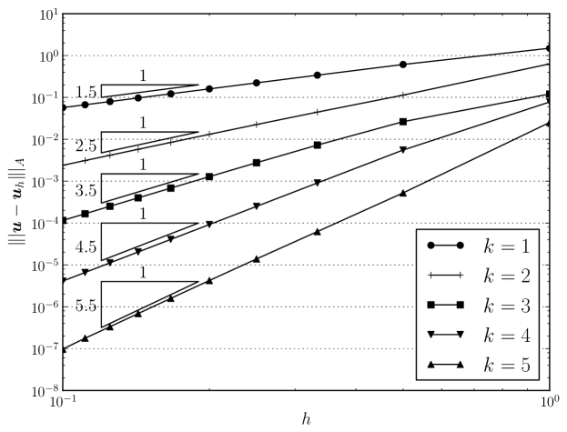
Fig. 1: Convergence for the hyperbolic case with $h$-refinement for various polynomial orders in $\left|\kern-0.9pt\left|\kern-0.9pt\left|\cdot\right|\kern-0.9pt\right|\kern-0.9pt\right|_{A}$.

For all polynomial orders the method converges robustly.

6.2 Elliptic problem

A problem on the domain $\Omega=\left({-1,1}\right)^{2}$ is now considered, with $\mu=0$, $\boldsymbol{a}=\left({0,0}\right)$ and $\kappa=1$. The source term $f$ is selected such that

$$u=\sin\left({\pi x}\right)\sin\left({\pi y}\right)$$ (108)

is the analytical solution to equation (1). The value of the penalty parameter is stated for each considered case.

The computed errors in the $L^{2}$ norm for $h$-refinement with elements of varying polynomial order and $\alpha=5$ are shown in Figure 2.

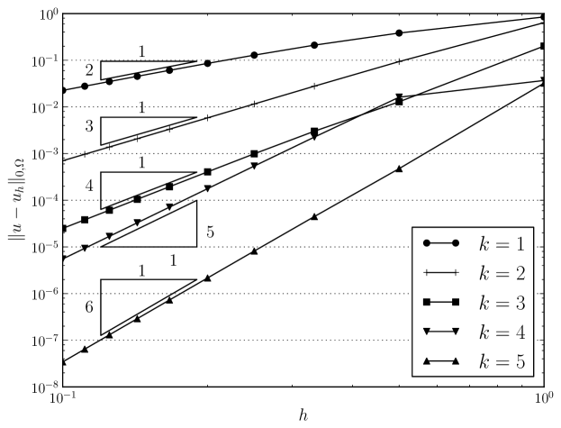
Fig. 2: Convergence for the elliptic case in $L^{2}$ with $h$-refinement for various polynomial orders and $\alpha=5$.

In all cases, the predicted $k+1$ order of convergence is observed. The computed results for $\alpha=6$ are shown in Figure 3, in which the convergence for the $k=2$ case is somewhat erratic.

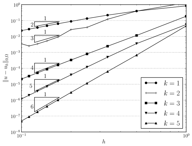
Fig. 3: Convergence for the elliptic case in $L^{2}$ with $h$-refinement for various polynomial orders and $\alpha=6$.

Using $\alpha=4k^{2}$, since the penalty parameter for the interior penalty method usually needs to be increased with increasing polynomial order, reliable convergence behaviour at the predicted rate is recovered, as can be seen in Figure 4.

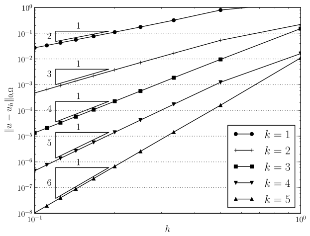
Fig. 4: Convergence for the elliptic case in $L^{2}$ with $h$-refinement for various polynomial orders and $\alpha=4k^{2}$.

6.3 Advection-diffusion problems

An advection-diffusion problem is considered on the domain $\Omega=\left({-1,1}\right)^{2}$, with $\mu=0$, $\boldsymbol{a}=\left({e^{x}(y\cos y+\sin y),e^{x}y\sin y}\right)$ and for various values of $\kappa$. The source term $f$ is chosen such that equation (108) is the analytical solution. For all cases, $\alpha=4k^{2}$.

The convergence behaviour is examined in terms of $\left|\kern-0.9pt\left|\kern-0.9pt\left|\boldsymbol{u}-\boldsymbol{u}_{h}\right|\kern-0.9pt\right|\kern-0.9pt\right|_{A}+\left|\kern-0.9pt\left|\kern-0.9pt\left|\boldsymbol{u}-\boldsymbol{u}_{h}\right|\kern-0.9pt\right|\kern-0.9pt\right|_{D}$. The computed error for the case $\kappa=1\times 10^{-3}$ is presented in Figure 5.

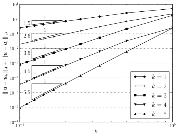
Fig. 5: Convergence for the advection-diffusion problem in $\left|\kern-0.9pt\left|\kern-0.9pt\left|\boldsymbol{u}-\boldsymbol{u}_{h}\right|\kern-0.9pt\right|\kern-0.9pt\right|_{A}+\left|\kern-0.9pt\left|\kern-0.9pt\left|\boldsymbol{u}-\boldsymbol{u}_{h}\right|\kern-0.9pt\right|\kern-0.9pt\right|_{D}$ for $\kappa=1\times 10^{-3}$ with $h$-refinement for various combinations of $k$ and $\alpha=4k^{2}$.

For this advection dominated problem, the method is observed to converge at the rate $k+1/2$. For $\kappa=0.1$, the observed convergence response is presented in Figure 6.

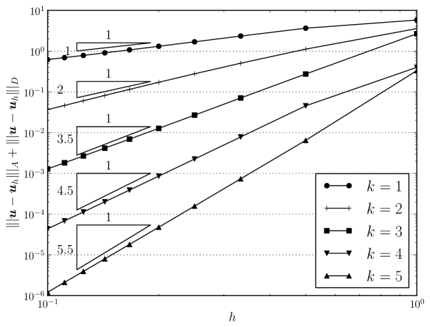
Fig. 6: Convergence for the advection-diffusion problem in $\left|\kern-0.9pt\left|\kern-0.9pt\left|\boldsymbol{u}-\boldsymbol{u}_{h}\right|\kern-0.9pt\right|\kern-0.9pt\right|_{A}+\left|\kern-0.9pt\left|\kern-0.9pt\left|\boldsymbol{u}-\boldsymbol{u}_{h}\right|\kern-0.9pt\right|\kern-0.9pt\right|_{D}$ for $\kappa=0.1$ with $h$-refinement for various combinations of $k$ and $\alpha=4k^{2}$.

A convergence rate of $k$ is observed for the lower order polynomial cases, and the rate appears approach $k+1/2$ for the higher-order polynomial cases. For $\kappa=10$, which is diffusion dominated, the observed convergence is presented in Figure 7.

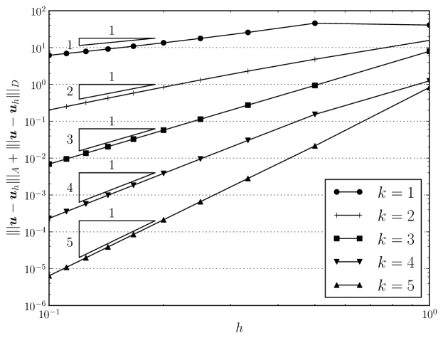
Fig. 7: Convergence for the advection-diffusion problem in $\left|\kern-0.9pt\left|\kern-0.9pt\left|\boldsymbol{u}-\boldsymbol{u}_{h}\right|\kern-0.9pt\right|\kern-0.9pt\right|_{A}+\left|\kern-0.9pt\left|\kern-0.9pt\left|\boldsymbol{u}-\boldsymbol{u}_{h}\right|\kern-0.9pt\right|\kern-0.9pt\right|_{D}$ for $\kappa=10$ with $h$-refinement for various combinations of $k$ and $\alpha=4k^{2}$.

As expected, a convergence rate of $k$ is observed for the diffusion-dominated case.

7 Conclusions

Stability and error estimates have been developed for an interface stabilised finite element method that inherits features of both continuous and discontinuous Galerkin methods. The analysis is for the hyperbolic and elliptic limit cases of the advection-diffusion-reaction equation. While the number of global degrees of freedom on a given mesh for the method is the same as for a continuous finite element method, the stabilisation mechanism is the same as that present in upwinded discontinuous Galerkin methods. This is borne out in the stability analysis, which demands consideration of an inf-sup condition. Analysis of the method shows that it inherits the stability properties of discontinuous Galerkin methods, and that it converges in $L^{2}$ at a rate of $k+1/2$ in the advective limit and $k+1$ in the diffusive limit, as is typical for discontinuous Galerkin and appropriately constructed stabilised finite element methods. The analysis presented in this work provides a firm theoretical basis for the method to support the performance observed in simulations in other works. The analysis results are supported by numerical examples which considered a range of polynomial order elements.

Acknowledgement

The author acknowledges the helpful comments on this manuscript from Robert Jan Labeur and the assistance of Kristian B. Ølgaard in implementing the features that facilitated the automated generation of the computer code used in Section 6.

References

- Hughes et al. [2006] T. J. R. Hughes, G. Scovazzi, P. B. Bochev, and A. Buffa. A multiscale discontinuous Galerkin method with the computational structure of a continuous Galerkin method. Computer Methods in Applied Mechanics and Engineering, 195(19-22):2761 – 2787, 2006.
- Labeur and Wells [2007] R. J. Labeur and G. N. Wells. A Galerkin interface stabilisation method for the advection-diffusion and incompressible Navier-Stokes equations. Computer Methods in Applied Mechanics and Engineering, 196(49–52):4985–5000, 2007.
- Cockburn et al. [2009] B. Cockburn, B. Dong, J. Guzmán, M. Restelli, and R. Sacco. A hybridizable discontinuous Galerkin method for steady-state convection-diffusion-reaction problems. SIAM Journal on Scientific Computing, 31(5):3827–3846, 2009.
- Burman and Stamm [2007] E. Burman and B. Stamm. Minimal stabilization for discontinuous Galerkin finite element methods for hyperbolic problems. Journal of Scientific Computing, 33(2):183–208, 2007.
- Labeur and Wells [2009] R. J. Labeur and G. N. Wells. Interface stabilised finite element method for moving domains and free surface flows. Computer Methods in Applied Mechanics and Engineering, 198(5-8):615 – 630, 2009.
- Buffa et al. [2006] A. Buffa, T. J. R. Hughes, and G. Sangalli. Analysis of a multiscale discontinuous Galerkin method for convection-diffusion problems. SIAM Journal on Numerical Analysis, 44(4):1420–1440, 2006.
- Ern and Guermond [2006] A. Ern and J.-L. Guermond. Discontinuous Galerkin methods for Friedrichs’ systems. I. General theory. SIAM Journal on Numerical Analysis, 44(2):753–778, 2006.
- Arnold et al. [2002] D. N. Arnold, F. Brezzi, B. Cockburn, and L. D. Marini. Unified analysis of discontinuous Galerkin methods for elliptic problems. SIAM Journal on Numerical Analysis, 39(5):1749–1779, 2002.
- Reed and Hill [1973] W. H. Reed and T. R. Hill. Triangular mesh methods for the neutron transport equation. Technical Report LA-UR-73-479, Los Alamos Scientific Laboratory, 1973.
- Lesaint and Raviart [1974] P. Lesaint and P.-A. Raviart. On a finite element method for solving the neutron transport equation. In Mathematical Aspects of Finite Elements in Partial Differential Equations, Publication No. 33, pages 89–123. Math. Res. Center, Univ. of Wisconsin-Madison, Academic Press, New York, 1974.
- Johnson and Pitkäranta [1986] C. Johnson and J. Pitkäranta. An analysis of the discontinuous Galerkin method for a scalar hyperbolic equation. Mathematics of Computation, 46(173):1–26, 1986.
- Wheeler [1978] M. F. Wheeler. An elliptic collocation-finite element method with interior penalties. SIAM Journal on Numerical Analysis, 15(1):152–161, 1978.
- Arnold [1982] D. N. Arnold. An interior penalty finite element method with discontinuous elements. SIAM Journal on Numerical Analysis, 19(4):742–760, 1982.
- Ern and Guermond [2004] A. Ern and J.-L. Guermond. Theory and Practice of Finite Elements, volume 159 of Applied Mathematical Sciences. Springer-Verlag, New York, 2004.
- Brenner and Scott [2008] S. C. Brenner and L. R. Scott. The Mathematical Theory of Finite Element Methods, volume 15 of Texts in Applied Mathematics. Springer New York, third edition, 2008.
- Evans [1998] L. C. Evans. Partial Differential Equations. American Mathematical Society, Providence, Rhode Island, 1998.
- Wells [2010] G. N. Wells. Supporting material, 2010. URL http://www.dspace.cam.ac.uk/handle/1810/226688.
- Kirby and Logg [2006] R. C. Kirby and A. Logg. A compiler for variational forms. ACM Transactions on Mathematical Software, 32(3):417–444, 2006.
- Ølgaard et al. [2008] K. B. Ølgaard, A. Logg, and G. N. Wells. Automated code generation for discontinuous Galerkin methods. SIAM Journal on Scientific Computing, 31(2):849–864, 2008.
- Ølgaard and Wells [2010] K. B. Ølgaard and G. N. Wells. Optimisations for quadrature representations of finite element tensors through automated code generation. ACM Transactions on Mathematical Software, 37(1):8:1–8:23, 2010.
- Logg and Wells [2010] A. Logg and G. N. Wells. DOLFIN: Automated finite element computing. ACM Transactions on Mathematical Software, 37(2):20:1–20:28, 2010.
- Bey and Oden [1996] K. S. Bey and J. T. Oden. hp-Version discontinuous Galerkin methods for hyperbolic conservation laws. Computer Methods in Applied Mechanics and Engineering, 133(3–4):259 – 286, 1996.
- Houston et al. [2000] P. Houston, C. Schwab, and E. Süli. Stabilized hp-finite element methods for first-order hyperbolic problems. SIAM Journal on Numerical Analysis, 37(5):1618–1643, 2000.