Next-to-eikonal corrections to soft gluon radiation: a diagrammatic approach

Abstract:

We consider the problem of soft gluon resummation for gauge theory amplitudes and cross sections, at next-to-eikonal order, using a Feynman diagram approach. At the amplitude level, we prove exponentiation for the set of factorizable contributions, and construct effective Feynman rules which can be used to compute next-to-eikonal emissions directly in the logarithm of the amplitude, finding agreement with earlier results obtained using path-integral methods. For cross sections, we also consider sub-eikonal corrections to the phase space for multiple soft-gluon emissions, which contribute to next-to-eikonal logarithms. To clarify the discussion, we examine a class of $\log(1-x)$ terms in the Drell-Yan cross-section up to two loops. Our results are the first steps towards a systematic generalization of threshold resummations to next-to-leading power in the threshold expansion.

1 Introduction

The eikonal approximation has played an important role throughout the history of gauge theory scattering amplitude calculations. It embodies the universal behavior of such amplitudes in the limit where massless gauge boson momenta become soft, and it encodes the semiclassical nature of soft, long-wavelength radiation. Early applications to potential scattering and Regge theory (see for example  [1, 2, 3]) predate the standard model of particle physics. In the context of modern applications to QED and QCD, the eikonal approximation is typically phrased in terms of Wilson lines: when radiated gauge bosons are soft, one may neglect the recoil of energetic particles; these can then be replaced by straight Wilson lines along the classical trajectories of the emitters (often called eikonal lines for this reason); this expresses the fact that soft gauge fields can affect energetic particles only by dressing them with a gauge phase. The fact that the eikonal approximation can be recast in terms of expectation values of (non-local) operators such as Wilson lines points to a deep connection between the perturbative and non-perturbative aspects of gauge theory scattering, a fact that was recently highlighted by remarkable results in maximally superymmetric ${\cal N}=4$ Yang-Mills theory (for a review, see [4]). Recent significant developments in the understanding of the all-order structure of infrared divergences in non-abelian gauge theories [5, 6, 7, 8] were also derived with the help of the special properties of the eikonal approximation.

A crucial feature of the eikonal approximation is the fact that scattering amplitudes exponentiate, which means that it is possible to establish a set of simplified rules to compute the logarithm of the amplitude. As a consequence, low-order perturbative calculations can be employed to gain access to all-order information, which is of great interest both for theory and for phenomenology. In QED, for example, a scattering amplitude ${\cal M}$ dressed with multiple soft photon emission may be written [9] in the schematic form

$${\cal M}\,=\,{\cal M}_{0}\,\exp\left[\sum G_{c}\right]\,,$$ (1)

where ${\cal M}_{0}$ is the amplitude without soft photon radiation, and the sum in the exponent is over connected Feynman diagrams for soft photon emission. Exponentiation was later shown to hold also for non-abelian gauge theory amplitudes [10, 11, 12], where however the structure of the exponent is more complicated, due to the non-commutativity of color matrices. The non-abelian analogue of eq. (1) for soft gluon emissions from two energetic (hard) partons connected by a color singlet vertex is

$${\cal M}\,=\,{\cal M}_{0}\,\exp\left[\sum\bar{c}_{W}\,W\right]\,,$$ (2)

where the sum in the exponent involves Feynman diagrams $W$ which are two-particle irreducible with respect to the hard emitting partons, and are called webs in the literature. The factors $\bar{c}_{W}$ are modified color factors, which differ from the conventional color factors $c_{W}$ associated with the same diagrams through the standard Feynman rules. Recently, eq. (2) was extended [13, 14] to more general multiparton amplitudes. In that case webs do not allow for a simple topological characterization, but it remains true that the logarithm of the amplitude can be computed in terms of a subset of Feynman diagrams with modified color factors.

The exponential structure of the amplitudes is a necessary ingredient for the resummation of soft gluon effects in many different high-energy cross sections. In general, in order to perform a resummation for a given observable, one must also require that the phase space for multiple soft gauge boson emission should factorize. If that happens, potentially large logarithms of ratios of physical scales, which often jeopardize the applicability of perturbation theory, can be resummed in exponential form. Soft gluon resummation is well understood, and has been widely investigated using a variety of techniques [15, 16, 17, 18, 19, 20, 21, 22, 23, 24, 25], leading to a vast array of phenomenological applications to many scattering processes in perturbative QCD. In this connection, it is important to recall that some of the large logarithms that arise in high-energy cross sections, for example when scattering takes place near a partonic threshold, originate from the emission of hard collinear gluons, and thus cannot be captured by the soft approximation. In what follows we will try to clearly distinguish these two effects.

The aim of this paper is to clarify the structure of next-to-eikonal (NE) contributions to scattering amplitudes (and eventually cross sections). For an amplitude involving $n$ soft gauge bosons with momenta $k_{i}$ ($i=1,\ldots,n$), we imagine rescaling all soft momenta by a common factor $\eta$. Then the eikonal approximation to the amplitude keeps the leading power in $\eta$ as $\eta\to 0$, which is typically $\eta^{-n}$ for an amplitude involving $n$ soft gauge bosons. The NE approximation organizes terms proportional to the next-to-leading power in this expansion, $\eta^{-(n-1)}$. Essentially, one takes $k_{i}\rightarrow 0$ for all but one gauge boson, whose momentum is kept to one power beyond the eikonal approximation. This eikonal expansion is related, but not identical, to the expansion of partonic cross sections near kinematic thresholds, which is used to organize Sudakov logarithms. Near partonic thresholds, one can typically parametrize the distance from threshold in terms of a single dimensionless variable $\xi$, such that $\xi\to 0$ is the threshold limit. Examples include $\xi=W^{2}/Q^{2}\sim(1-x_{\rm Bj})$ in DIS, $\xi=1-Q^{2}/s$ in Drell-Yan, and $\xi=1-T$ for, say, the thrust distribution in electron-positron annihilation. In all these cases, the partonic differential cross section receives contributions of the form

$$\frac{d\sigma}{d\xi}\,=\,\sum_{n=0}^{\infty}\sum_{m=0}^{2n-1}\alpha_{s}^{n}\left[a_{nm}\frac{\log^{m}(\xi)}{\xi}+b_{nm}\log^{m}(\xi)+{\cal O}(\xi)\right]\,.$$ (3)

We call the expansion in powers of $\xi$ in eq. (3) a “threshold” expansion. In this terminology, NE corrections to scattering amplitudes start contributing at the level of $b_{nm}$ terms, that is at next-to leading order in the threshold expansion (NLT). On the other hand, in the presence of final-state jets of hard particles, there are hard collinear emissions in the matrix elements which contribute at NLT but are not captured by the eikonal expansion: they must be dealt with using collinear evolution equations. NLT contributions can be phenomenologically important (see for example [26]) and are conceptually interesting since they probe the reach of the universal properties of soft and collinear radiation. As a consequence, these contributions have been recently studied in some detail: Ref. [27] showed how $\xi$-independent terms completely exponentiate for simple color-singlet QCD cross-sections (see also [28, 29]); subsequently, Ref. [30] proposed a modification of collinear evolution equations that allows the exponentiation of a subset of NLT terms; this was exploited in Ref. [31] to propose an ansatz for NLT Sudakov resummation for color-singlet QCD cross sections, that was shown to reproduce the bulk of these contributions through NNLO. Other studies [32, 33, 34, 35, 36, 37, 38] have uncovered intriguing relations between the coefficients of NLT contributions in finite order calculations, and have proposed all-order generalizations. The ultimate goal of our work, as well as of Refs. [39, 40], is to reach a complete understanding of NLT terms and organize them in resummed form to the extent to which this is possible. For cross sections, this will also require an understanding of multi-gluon phase space beyond the eikonal approximation, and some progress in this direction is described already in this paper.

As a first step in this program, we intend to establish to what extent the exponentiation properties of the eikonal approximation extend to NE level, and eventually to derive effective Feynman rules and iterative methods to compute directly the perturbative exponent to the required accuracy. Our results will reproduce and clarify from a diagrammatic viewpoint those obtained in [39], where the problem of NE contributions was first considered using path integral methods. In that paper, a factorised form was assumed for Green functions with a fixed number of hard outgoing particles, which may emit any number of soft gluons. By recasting the propagators for the external particles (in the background of a soft gauge field) in terms of first-quantised path integrals, an effective field theory for the soft gauge field arises, with source vertices localised along the external lines. Within that formalism, exponentiation of soft photon contributions (in an abelian field theory) was shown to be straightforwardly related to the exponentiation of connected diagrams in quantum field theory. In the non-abelian case, the field theory for the soft gauge field was more complicated, due to the fact that the source terms are matrix-valued in color space and, thus, non-commuting. It was, however, possible to ascertain that a subset of diagrams (indeed the webs of [12]) does exponentiate. The exponentiation derived in [39] leaves out those contributions to the matrix elements that violate the assumed factorization properties of the correlators. We similarly observe that our analysis applies to both real and virtual gluons, provided all emissions can be considered soft with respect to hard scale of the problem; in the case of hard virtual gluons, however, the known factorization properties of soft radiation do not fully generalize to NE level, and there are further contributions arising from soft gluons emitted by lines internal to the hard subamplitude. Here we will concentrate on the structure of factorizable contributions, which do exponentiate.

To be specific, the diagrammatic techniques developed in the present paper, in agreement with the final result of [39], organize next-to-eikonal contributions to matrix elements in the schematic form

$${\cal M}\,=\,{\cal M}_{0}\,\exp\left[{\cal M}_{\rm eik}+{\cal M}_{\text{NE}}\right]\,(1+{\cal M}_{r})+{\cal O}\left({\rm NNE}\right)\,.$$ (4)

Here ${\cal M}_{0}$ is the Born contribution, and ${\cal M}_{{\rm eik},\,\text{NE}}$ collect factorizable contributions due to emissions of soft gluons external to the hard interaction. Non-factorizable contributions, arising from internal emission graphs, are collected in the function ${\cal M}_{r}$. This contribution does not formally exponentiate, but has an iterative structure to all orders in perturbation theory. At NE level, as suggested in [39], non-factorizable contributions can be organized by means of the Low-Burnett-Kroll theorem [41, 42], as extended in [43] to encompass collinear divergences. In the present paper, we neglect non-factorizable contrbutions contained in ${\cal M}_{r}$ and concentrate on the structure of the exponent in eq. (4) at NE level. Note that Ref. [39] addressed explicitly the case of two external hard partons connected by a color-singlet interaction. The structure of the exponent in the case of multi-parton amplitudes was recently examined in [13, 14], including a first analysis of next-to-eikonal corrections using path integral methods in [13].

We emphasize that the diagrammatic analysis presented in this paper is a necessary step, not only in order to test the results derived with path-integral methods in [39], but also in order to place these results in the context of general proofs of factorization theorems, and to clarify the precise limits of applicability of the formalism. As an example, the factorization arguments organizing Low’s theorem contributions at NE level in Ref. [43] are formulated in diagrammatic language, and a proper matching with factorizable contributions in order to avoid double counting must also employ diagrammatic techniques. Similarly, possible extensions of this formalism to collinear contributions at next-to-leading order in the threshold expansion will need to be mapped to existing diagrammatic analyses. Our results thus strengthen the validity of the conclusions reached by the path integral method, and place them in the more general context of factorization studies with diagrammatic methods.

In order to test our results and to illustrate and clarify our technique in a concrete application, in the last part of this paper we consider a subset of the real-emission contributions to the Drell-Yan cross section up to NNLO. Processes involving parton annihilation into an electroweak final state, such as Drell-Yan or weak boson production, or Higgs production in the gluon fusion channel, are ideal testing grounds for our formalism: indeed, near threshold all radiation in these processes is soft, so that one does not need to worry about hard collinear emissions. Furthermore, by considering real emission diagrams only, we don’t need to include non-factorizable contributions related to Low’s theorem, and therefore we should be able to reproduce exactly the fixed-order results upon applying our effective Feynman rules at the level of the exponent. We perform this test on abelian-like contributions (proportional to $C_{F}^{n}$ in QCD) up to two loops (the first non-trivial order where exponentiation has an impact), finding the expected result. Applying our formalism to a hadronic cross section forces us to tackle the issue of the factorizability of soft gluon phase space, and we present some preliminary results suggesting that the factorization properties of the eikonal phase space may admit a simple generalization at NE level.

The structure of the paper is as follows. In Sec. 2 we review the derivation of the exponentiation of soft corrections in the abelian and non-abelian cases, using an iterative Feynman diagram method. In Sec. 3 we derive effective Feynman rules for NE emissions. Crucial to this result is the fact that the sum over all NE diagrams has a factorisable form. In Sec. 4 we then demonstrate the exponentiation of NE corrections, extending the methods used in Sec. 2. In Sec. 5 we perform a detailed comparison of the rules thus obtained with the results found using the path integral method of [39]. Finally, in Sec. 6 we present the application of the ideas derived in this paper to the case of Drell-Yan production. In Sec. 7 we briefly summarize our results, while some technical aspects are discussed in the Appendices: notably, Appendix B discusses the structure of phase space for multiple soft gluon emission at arbitrary order, providing arguments for a form of factorization that could be applied at NE level.

2 Introduction to eikonal exponentiation

Exponentiation of soft gauge boson corrections at the eikonal level was first demonstrated for abelian gauge theories in [9], and later generalised to non-abelian theories in [10, 11, 12]. Here we review the derivation of this result using Feynman diagram methods (see also [44] for a pedagogical exposition), both in order to make our paper reasonably self-contained and to introduce methods and notations that will prove useful when generalising the results to NE order.

The proof of exponentiation is two-fold. First, one establishes a set of effective Feynman rules in the eikonal approximation, showing that they capture the leading-power behavior of the amplitude as soft momenta become vanishingly small, to all orders in perturbation theory; then one uses these effective Feynman rules to classify a subset of Feynman diagrams that generate the full eikonal amplitude upon exponentiation. We will do this first for the simple case of an abelian theory, and then discuss the non-trivial modifications that are necessary in the nonabelian case.

2.1 Abelian eikonal exponentiation

In order to derive the eikonal Feynman rules it is sufficient to consider a single hard massless external line of final on-shell momentum $p$, originating from some unspecified hard interaction described by a matrix element ${\cal M}_{0}(p)$. The hard line may emit a number $n$ of soft photons with momenta $k_{i}$, as depicted in fig. 1, where we choose the ordering so that momentum $k_{1}$ is emitted closest to the hard interaction.

Figure 1: Soft photon emission from an energetic line.

If the emitting particle is a Lorentz scalar, such an external line dresses the hard interaction according to

$${\cal M}^{\mu_{1}\ldots\mu_{n}}(p,k_{i})={\cal M}_{0}(p)\,\frac{1}{(p+K_{1})^{2}}(2p+K_{1}+K_{2})^{\mu_{1}}\ldots\frac{1}{(p+K_{n})^{2}}(2p+K_{n})^{\mu_{n}}\,,$$ (5)

where we have introduced the partial momentum sums $K_{i}=\sum_{m=i}^{n}k_{m}$.

The eikonal approximation in this case can simply be defined as the leading-power contribution to the amplitude when the photon momenta $k_{i}^{\mu_{i}}\to 0$, $\forall i$. In this limit, eq. (5) becomes

$${\cal M}^{\mu_{1}\ldots\mu_{n}}(p,k_{i})={\cal M}_{0}(p)\,\frac{p^{\mu_{1}}\ldots p^{\mu_{n}}}{(p\cdot K_{1})\ldots(p\cdot K_{n})}\,.$$ (6)

If the emitter is a Dirac fermion, eq. (5) becomes

$${\cal M}^{\mu_{1}\ldots\mu_{n}}(p,k_{i})={\cal M}_{0}(p)\,\frac{\not{p}+\not{K}_{1}}{(p+K_{1})^{2}}\gamma^{\mu_{1}}\ldots\frac{\not{p}+\not{K}_{n}}{(p+K_{n})^{2}}\gamma^{\mu_{n}}u(p)\,,$$ (7)

where $u(p)$ is the spinor associated with the final state on-shell particle. At leading power in the soft momenta, this reduces to

$${\cal M}^{\mu_{1}\ldots\mu_{n}}(p,k_{i})={\cal M}_{0}(p)\,\frac{\not{p}}{2p\cdot K_{1}}\gamma^{\mu_{1}}\ldots\frac{\not{p}}{2p\cdot K_{n}}\gamma^{\mu_{n}}u(p).$$ (8)

This appears to be more complicated than the scalar case due to the non-trivial spinor structure. One may however use the anticommutation properties of Dirac matrices and the Dirac equation to reduce eq. (8) precisely to the form of eq. (6), with the spinor $u(p)$ reabsorbed into the radiationless matrix element ${\cal M}_{0}(p)$. The eikonal factor is the same in both cases, displaying the well-known result that the eikonal approximation is insensitive to the spin of the emitting particles. One may also notice that the eikonal factor does not depend on the energy of the emitter, since it is invariant under rescalings of the hard momentum $p^{\mu}$: at leading power in the soft momenta, one is effectively neglecting the recoil of the hard particle against soft radiation.

The eikonal factor can be further simplified by employing Bose symmetry. Indeed, in constructing any physical quantity depending on the amplitude ${\cal M}^{\mu_{1}\ldots\mu_{n}}(p,k_{i})$, one will need to sum over all diagrams corresponding to permutations of the emitted photons along the hard line. Having done this, the eikonal factor multiplying ${\cal M}_{0}(p)$ on the r.h.s. of eq. (6) will be replaced by the symmetrized expression

$$E^{\mu_{1}\ldots\mu_{n}}(p,k_{i})\,=\,\frac{1}{n!}\,p^{\mu_{1}}\ldots p^{\mu_{n}}\,\sum_{\pi}\frac{1}{p\cdot k_{\pi_{1}}}\frac{1}{p\cdot(k_{\pi_{1}}+k_{\pi_{2}})}\,\ldots\,\frac{1}{p\cdot(k_{\pi_{1}}+\ldots+k_{\pi_{n}})}\,,$$ (9)

where the sum is over all permutations of the photon momenta, and $k_{\pi_{i}}$ is the $i^{\text{th}}$ momentum in a given permutation. There are $n!$ permutations, and each gives the same contribution to any physical observable. This becomes manifest using the eikonal identity

$$\sum_{\pi}\frac{1}{p\cdot k_{\pi_{1}}}\frac{1}{p\cdot(k_{\pi_{1}}+k_{\pi_{2}})}\ldots\frac{1}{p\cdot(k_{\pi_{1}}+\ldots k_{\pi_{n}})}=\prod_{i}\frac{1}{p\cdot k_{i}}\,.$$ (10)

Using eq. (10), the eikonal factor $E^{\mu_{1}\ldots\mu_{n}}(p,k_{i})$ arising from $n$ soft emissions on an external hard line becomes simply

$$E^{\mu_{1}\ldots\mu_{n}}(p,k_{i})\,=\,\prod_{i}\,\frac{p^{\mu_{i}}}{p\cdot k_{i}}\,,$$ (11)

which is manifestly Bose symmetric and invariant under rescalings of the momenta $\{p_{i}\}$. In practice, each eikonal emission can be expressed by the effective Feynman rule

      $${\,=\,\,\,\Large\frac{p^{\mu}}{p\cdot k}}$$ (12)

As is well known, these Feynman rules can be obtained by replacing the hard external line with a Wilson line along the classical trajectory of the charged particle. In abelian quantum field theories this is given by the operator

$$\Phi_{\beta}(0,\infty)=\exp\left[\,{\rm i}e\int_{0}^{\infty}d\lambda\,\beta\cdot A(\lambda\beta)\,\right]~{},$$ (13)

where $\beta$ is the dimensionless four-velocity corresponding to the momentum $p$. This expresses the fact that soft emissions affect the hard particle only by dressing it with a gauge phase.

Figure 2: A process involving two eikonal lines A and B, interacting through the exchange of soft gluons forming diagram $G$.

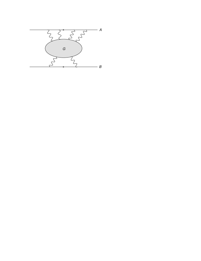
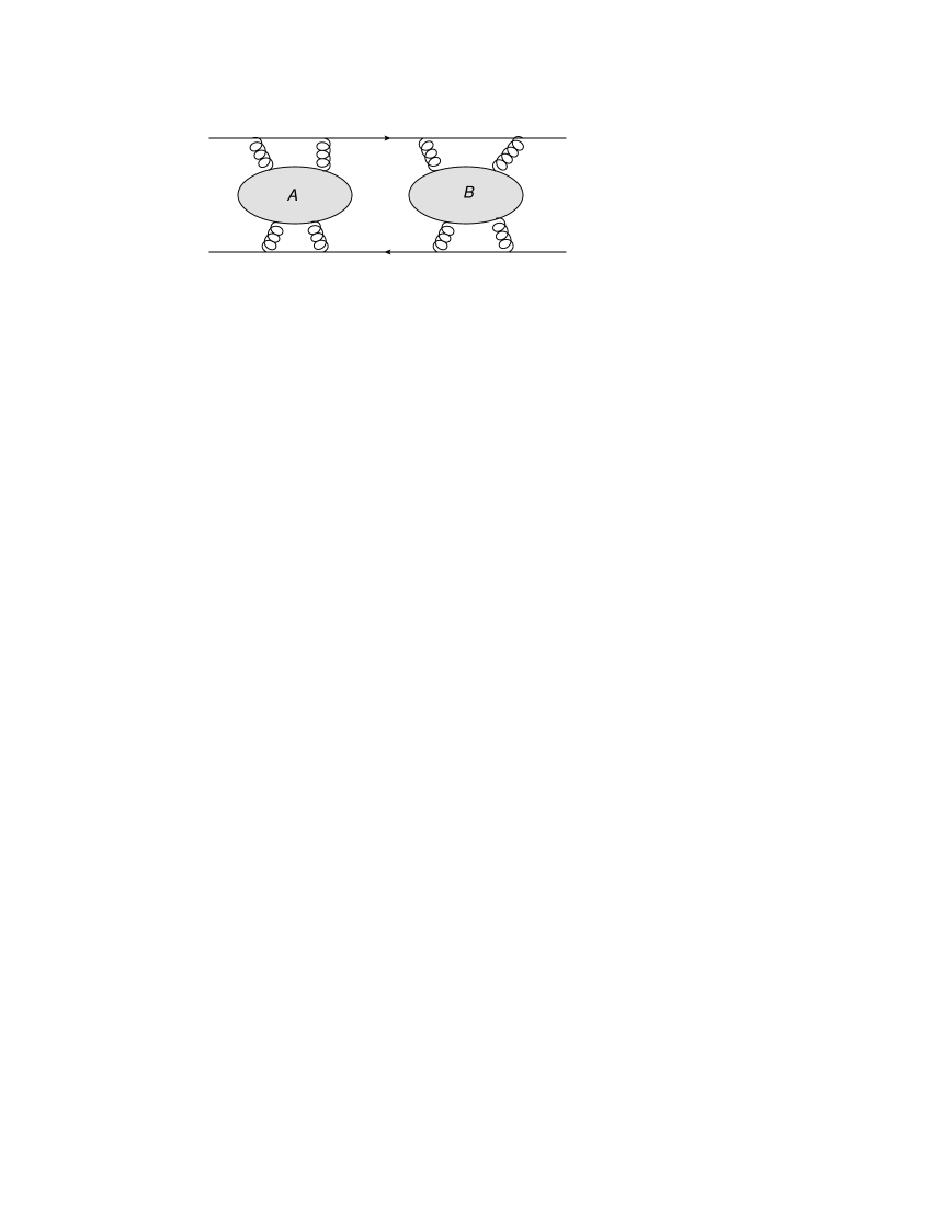
Having constructed the effective Feynman rules, one may proceed to demonstrate the exponentiation of soft photon corrections as follows. As an example, we consider graphs of the form shown in fig. 2, at a fixed order in the perturbative expansion. Fig. 2 consists of two eikonal lines, labelled $A$ and $B$, each of which emits a number of soft photons. Notice that although we consider only two eikonal lines here, the analysis below generalises to any number of hard charged particles. One may envisage lines $A$ and $B$ as emerging from a hard interaction, and one may consider the graph $G$ either as a contribution to an amplitude, or to a squared amplitude (in which case some of the propagators in $G$ will be cut).

Diagram $G$ can be taken as consisting only of soft photons and fermion loops: in fact, at leading power in the soft momenta, soft photons originating from the hard scattering give no contribution (a statement which will have to be revisited when including NE corrections). Photons originating from one of the two eikonal lines must land on the other one, or on a fermion loop inside $G$. Indeed, a photon cannot land on the same eikonal line, as in that case the diagram is proportional to $p^{\mu}p_{\mu}=0$.

Using eikonal Feynman rules, one finds that graphs of the form of fig. 2 contribute to the corresponding (squared) amplitude a factor

$${\cal F}_{AB}\,=\,\sum_{G}\,\left[\prod_{i}\frac{p_{A}^{\mu_{i}}}{p_{A}\cdot k_{i}}\right]\left[\prod_{j}\frac{p_{B}^{\nu_{j}}}{p_{B}\cdot l_{j}}\right]G_{\mu_{1}\ldots\mu_{n};\nu_{1}\ldots\nu_{m}}(k_{i},l_{j})\,,$$ (14)

where $k_{i}$, $l_{j}$ are the momenta of the photons emitted from lines $A$ and $B$ respectively, with $i=1,\ldots,n$ and $j=1,\ldots,m$.

Given that we have already summed over permutations in order to obtain the eikonal Feynman rules, each diagram $G$ can be uniquely specified by the set of connected subdiagrams it contains, as indicated schematically in fig. 3, where each possible connected subdiagram $G_{c}^{(i)}$ occurs $N_{i}$ times. According to the standard rules of perturbation theory, diagram $G$ has a symmetry factor corresponding to the number of permutations of internal lines which leave the diagram invariant. This symmetry factor is given by

$$S_{G}=\prod_{i}\,S_{i}^{N_{i}}\,(N_{i})!\,,$$ (15)

where $S_{i}$ is the symmetry factor associated with each connected subdiagram $G_{c}^{(i)}$, and the factorials account for permutations of identical connected subdiagrams, which must be divided out. Contracting Lorentz indices as in eq. (14), the eikonal factor ${\cal F}_{AB}$ may be written as

$${\cal F}_{AB}\,=\,\sum_{\{N_{i}\}}\,\prod_{i}\,\frac{1}{N_{i}!}\,\left[{\cal F}_{c}^{(i)}\right]^{N_{i}}\,,$$ (16)

where

$${\cal F}_{c}^{(i)}\,=\,\frac{1}{S_{i}}\,\left(\prod_{q}\frac{p_{A}^{\mu_{q}}}{p_{A}\cdot k_{q}}\right)\left(\prod_{r}\frac{p_{B}^{\nu_{r}}}{p_{B}\cdot l_{r}}\right)G^{(i)}_{\mu_{1}\ldots\mu_{n_{q}};\nu_{1}\ldots\nu_{m_{r}}}(k_{q},l_{r})$$ (17)

is the expression for each connected subdiagram, including the appropriate symmetry factor. Recognising eq. (16) as an exponential series, it follows that

$${\cal F}_{AB}\,=\,\exp\left[\sum_{i}{\cal F}_{c}^{(i)}\right]\,.$$ (18)

We conclude that soft photon corrections exponentiate in the eikonal approximation, and the exponent is given by the sum of all connected subdiagrams.

Figure 3: Decomposition of a soft photon graph into connected subdiagrams $G_{c}^{(i)}$, each of which occurs $N_{i}$ times.

The same result was recently rederived in [39], using path integral methods to derive soft photon exponentiation from the well-understood exponentiation of disconnected diagrams in quantum field theory.

2.2 Non-abelian eikonal exponentiation

We now consider the generalisation of eikonal exponentiation to non-abelian theories. The results are well known [11, 12], but we will introduce methods and notation that will prove useful in the extension to NE order. We will examine the case of two incoming or outgoing hard emitting particles connected by a color-singlet hard interaction, as happens for example in Drell-Yan production, deep inelastic scattering or $e^{+}e^{-}$ annihilation. We note that the results below extend to multiple hard colored emitters, as recently shown in Refs. [13, 14].

The proof of the abelian result relies crucially on the application of the eikonal identity after summing over the permutations of all photon momenta on each eikonal line. In the nonabelian case, this identity cannot be used, due to the presence of non-commutative color matrices associated with each emission. Exponentiation, however, is still possible, but with a somewhat more complicated structure.

Figure 4: Decomposition of a higher order non-Abelian diagram in terms of webs.

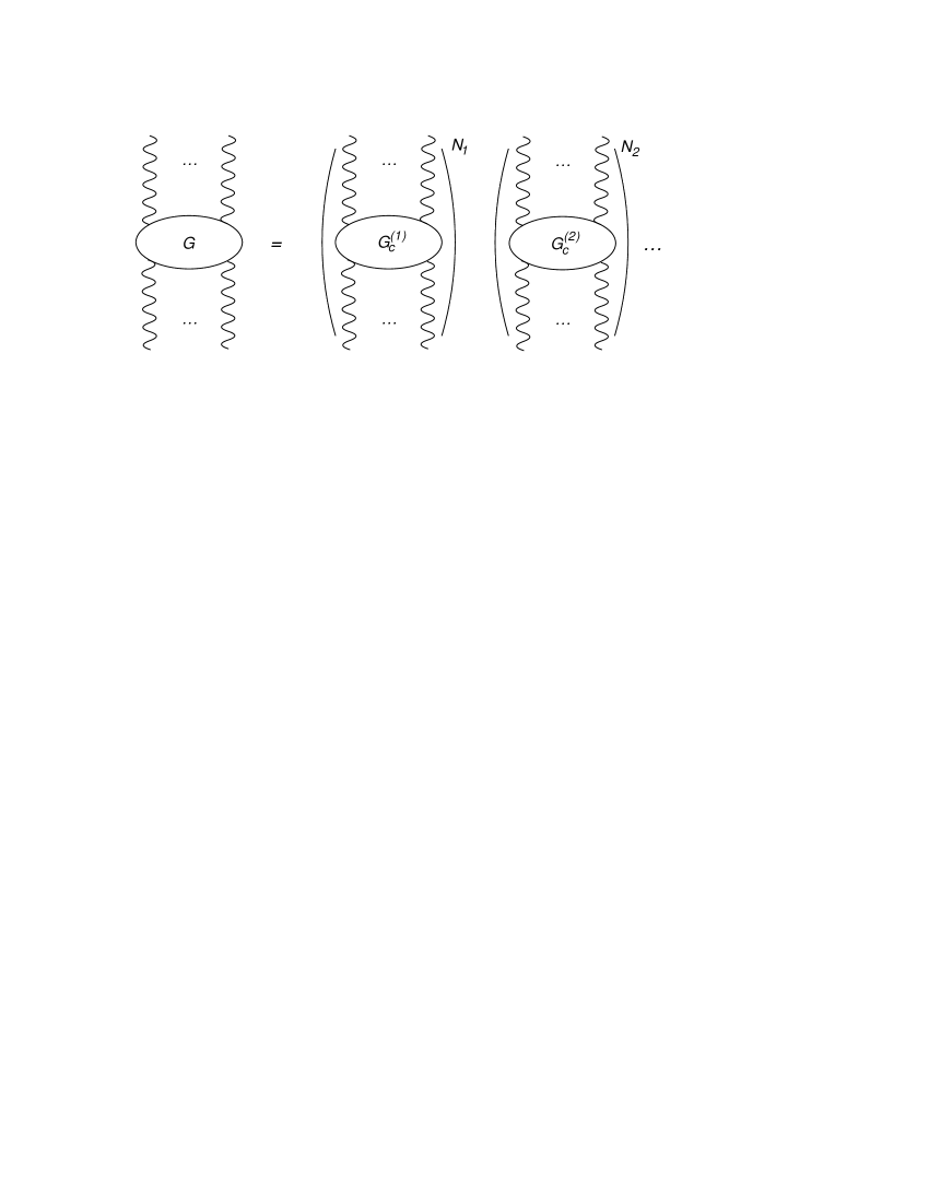
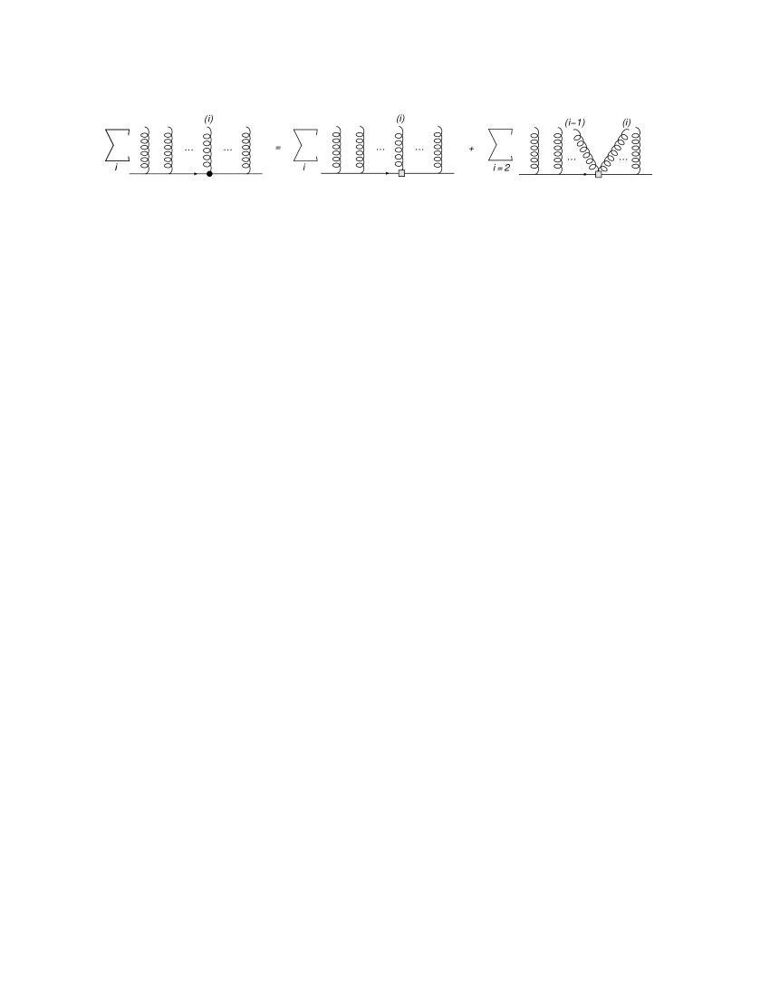
First we introduce the concepts of webs and groups. A web is a two-eikonal irreducible diagram, i.e. a diagram that cannot be disconnected by cutting the two eikonal lines. Higher order diagrams can be rewritten as sums of products of webs: an example is illustrated in fig. 4, which shows a particular fourth order diagram that is not a web, and its subsequent decomposition into webs.

A group is the projection of a web onto a single eikonal line: therefore, gluons emitted from an eikonal line belong to the same group if they belong to the same web. This is illustrated in fig. 5, where we depict the groups that result on the lower eikonal line from the webs of fig. 4.

Figure 5: Gluon groups obtained from the lower eikonal line of fig. 4, with the same color coding as in that figure.

Having introduced the concept of a group, one observes a useful generalisation of the eikonal identity, eq. (10), to sums over permutations that do not affect the ordering of gluons within groups [12, 44]. Let $\tilde{\pi}$ be a permutation of the gluons (with momenta $\{k_{i}\}$) emitted by a given eikonal line of momentum $p$, with the restriction that the ordering of the gluons in each group $g$ be held fixed. Then one may write

$$\sum_{\tilde{\pi}}\,\frac{1}{p\cdot k_{\tilde{\pi}_{1}}}\frac{1}{p\cdot(k_{\tilde{\pi}_{1}}+k_{\tilde{\pi}_{2}})}\,\ldots\,\frac{1}{p\cdot(k_{\tilde{\pi}_{1}}+\ldots+k_{\tilde{\pi}_{n}})} \,=\,\prod_{{\rm groups}\,\,g}\,\,\frac{1}{p\cdot k_{g_{1}}}\frac{1}{p\cdot(k_{g_{1}}+k_{g_{2}})}$$

$$\qquad\ldots\,\frac{1}{p\cdot(k_{g_{1}}+\ldots+k_{g_{m}})}\,.$$ (19)

Here $k_{\tilde{\pi}_{i}}$ and $k_{g_{i}}$ are the momenta of the $i^{\text{th}}$ gluon in permutation $\tilde{\pi}$ and group $g$, respectively, where $g$ contains, say, $m$ gluons. As an example of this result, consider an eikonal line with 3 gluon emissions, where gluons 1 and 2 belong to one group, and gluon 3 to another one; then, eq. (19) amounts to the statement

$$\frac{1}{p\cdot k_{1}}\frac{1}{p\cdot(k_{1}+k_{2})}\frac{1}{p\cdot(k_{1}+k_{2}+k_{3})}\,+\,\frac{1}{p\cdot k_{1}}\frac{1}{p\cdot(k_{1}+k_{3})}\frac{1}{p\cdot(k_{1}+k_{3}+k_{2})}$$

$$\qquad+\,\frac{1}{p\cdot k_{3}}\frac{1}{p\cdot(k_{3}+k_{1})}\frac{1}{p\cdot(k_{3}+k_{1}+k_{2})}\,=\,\frac{1}{p\cdot k_{3}}\,\left(\frac{1}{p\cdot k_{2}}\frac{1}{p\cdot(k_{1}+k_{2})}\right)\,.$$ (20)

The RHS displays the factorization of gluons from different groups. Henceforth, unless otherwise stated, all permutations of gluon momenta involve fixed orderings of the gluons inside each group; thus we drop the tilde on the permutation symbols $\tilde{\pi}$ for brevity.

Next we examine contractions of soft gluons emanating from two emitting lines connected by a color singlet hard interaction. A given diagram $G$ connecting the external lines then has two color indices in some representation of the non-abelian gauge group, one index for each eikonal line. Color conservation forces the color structure of each diagram to be proportional to the identity matrix $\delta_{ij}$, where $i$ and $j$ are indices in the chosen representation. Denote by $\text{E}(G)$ the eikonal amplitude arising from diagram $G$, not including color matrices. $\text{E}(G)$ encodes the momentum information carried by a particular diagram, but not its color structure: we can then write the factor contributed by $G$ to the (squared) matrix element as

$${\cal F}_{G}\,=\,c_{G}\,\delta_{ij}\,\text{E}(G)\,,$$ (21)

where $c_{G}$ is the color factor associated with $G$, and for simplicity we are not displaying the internal Lorentz structure. This notation allows us to rewrite eq. (19) in a more formal and useful way. Consider two soft gluon diagrams $H_{1}$ and $H_{2}$, connecting the same two eikonal lines $A$ and $B$. One may define the product of these two eikonal diagrams, using eq. (19) in reverse, as

$$\text{E}(H_{1})\,\text{E}(H_{2})\,=\,\sum_{\pi_{A}}\,\sum_{\pi_{B}}\,\text{E}(H_{1}\cup_{\pi_{A}}^{\pi_{B}}H_{2})\,,$$ (22)

where $H_{1}\cup_{\pi_{A}}^{\pi_{B}}H_{2}$ denotes the particular merging that results from combining $H_{1}$ and $H_{2}$ so that the gluon permutations on the eikonal lines are given by $\pi_{A}$ and $\pi_{B}$ respectively. Note that there may be a different number of gluons on each external line. An example of this is shown in fig. 6.

$$\begin{array}[]{ccccc}\includegraphics{merge1}&\bigcup_{132}^{12}&\includegraphics{merge2}&=&\includegraphics{merge3}\end{array}$$

Figure 6: Illustration of the merging product $\cup_{\pi_{A}}^{\pi_{B}}$ between two eikonal graphs, where $\pi_{A}$ and $\pi_{B}$ are permutations of the gluons on eikonal lines $A$ and $B$ such that ordering within each group is held fixed.

Each possible merging of $H_{1}$ and $H_{2}$ gives some diagram $G$. The same diagram $G$ could however result from different mergings that arise from different permutations $\pi_{A}$, $\pi_{B}$. One may then rewrite eq. (22) more formally as

$$\text{E}(H_{1})\,\text{E}(H_{2})\,=\,\sum_{G}\,\text{E}(G)\,N_{G|H_{1}H_{2}}\,,$$ (23)

where the multiplicity $N_{G|H_{1}H_{2}}$ denotes the number of ways in which diagram $G$ can be generated from mergings of $H_{1}$ and $H_{2}$. Equation (23) generalises immediately to the product of any number of eikonal subdiagrams, as

$$\text{E}(H_{1})^{s_{1}}\,\text{E}(H_{2})^{s_{2}}\,\ldots\,\text{E}(H_{n})^{s_{n}}\,=\,\sum_{G}\,\text{E}(G)\,N_{G|H_{1}^{s_{1}}H_{2}^{s_{2}}\ldots H_{n}^{s_{n}}}\,,$$ (24)

where each diagram $H_{i}$ occurs $s_{i}$ times in the product.

With these notations in hand, we are now ready to state the exponentiation theorem for nonabelian eikonal diagrams. Consider the exponential

$$\exp\left\{\sum_{H}\,\bar{c}_{H}\,\text{E}(H)\right\}\,,$$ (25)

where the sum is over all diagrams $H$, each with an accompanying color factor $\bar{c}_{H}$ whose interpretation will become clear in what follows (the bar is used to distinguish these color factors from those arising from conventional Feynman rules, $\{c_{H}\}$). Note that each $H$ may be decomposable in terms of products of smaller subdiagrams. Using eq. (24), one may then write

$$\exp\left\{\sum_{H}\,\bar{c}_{H}\,\text{E}(H)\right\}\,=\,\prod_{H}\left(\sum_{n}\frac{1}{n!}\left[\bar{c}_{H}\,\text{E}(H)\right]^{n}\right)\,=\,\sum_{G}\,c_{G}\,\text{E}(G)\,,$$ (26)

where the sum on the right-hand side is again over all possible diagrams $G$ (i.e. we use a different label on the left- and right-hand sides), and $\{c_{G}\}$ are constants. Expanding the exponential, one generates all possible products of diagrams. Each such product is itself equal to a linear combination of diagrams, by eq. (24), and thus contributes to various terms on the right-hand side of eq. (26). Each diagram $H$ in the exponent thus appears on the right-hand side of eq. (26) in two ways: either as itself (i.e. contributing only to the term where $G$ is equal to $H$), or as a component of larger diagrams $G$. One may then equate coefficients on the left- and right- hand sides of eq. (26), so that the choice of constants $\{c_{G}\}$ uniquely fixes, at least in principle, the constants $\{\bar{c}_{H}\}$. Our choice is to require that the constants $\{c_{G}\}$ on the right-hand side of eq. (26) be the usual color factors of perturbation theory. We can then show that the constants $\{\bar{c}_{H}\}$ are zero except for a subset of diagrams $H$ which have the property of being two-eikonal-line irreducible. These are the webs of [11, 12], that were referred to at the beginning of this section.

One proceeds as follows. First one notes, as we just discussed, that each diagram $G$ has a set of decompositions into subdiagrams $H$. This includes the case where $G$ cannot be decomposed into smaller parts, and thus has only the trivial decomposition where $H$ is equal to $G$ itself. An example of how a simple diagram can be decomposed is shown in fig. 7. Each decomposition can be uniquely labelled by a set of integers $\{m_{H}\}$ that specify how many times each subdiagram $H$ occurs in the decomposition of $G$. In the simple example shown in fig. 7, there are two decompositions labelled by $\{m_{\bf I},m_{\bf X}\}=\{2,0\}$ and $\{0,1\}$, where the notation $m_{{\bf I,X}}$ is suggested by the figure. To make use of this decomposition, we note that one can rearrange the expansion of any product of exponentials, such as the one appearing in eq. (26), as

$$\prod_{H}\left(\sum_{n}\frac{1}{n!}\,\big{[}\bar{c}_{H}\,\text{E}(H)\big{]}^{n}\right)=\sum_{\{p_{H}\}}\prod_{H}\frac{1}{p_{H}!}\,\big{[}\bar{c}_{H}\,\text{E}(H)\big{]}^{p_{H}}\,.$$ (27)

In the present context, each dummy index $p_{H}$ can be interpreted precisely as the multiplicity $m_{H}$ of subdiagram $H$ in graph $G$.

$$\raisebox{-20.2322pt}{\includegraphics{diagramX}}\rightarrow\left\{\left\{\raisebox{-20.2322pt}{\includegraphics{diagramI}},\raisebox{-20.2322pt}{\includegraphics{diagramI}}\right\}\,,\left\{\raisebox{-20.2322pt}{\includegraphics{diagramX}}\right\}\right\}$$

Figure 7: A diagram and its set of decompositions. The first decomposition has $m_{{\bf I}}=2$ and $m_{\bf X}=0$, the second decomposition has $m_{{\bf I}}=0$ and $m_{\bf X}=1$.

We can now exploit eq. (24) to rewrite each product of subgraphs in eq. (27) as a single sum over graphs. Equation (27) then becomes

$$\prod_{H}\left(\sum_{n}\frac{1}{n!}\,\big{[}\bar{c}_{H}\,\text{E}(H)]^{n}\right)\,=\,\sum_{G}\,\text{E}(G)\,\sum_{\{m_{H}\}}N_{G|\{m_{H}\}}\left(\prod_{H}\frac{1}{m_{H}!}\,\bar{c}_{H}^{\,m_{H}}\right)\,,$$ (28)

where we denote by $N_{G|\{m_{H}\}}$ the number of ways in which diagram $G$ can be formed out of the given decomposition specified by $\{m_{H}\}$. The expression now has the form of a single sum over all diagrams $G$ (weighted by non-trivial coefficients), and thus can be matched to the right-hand side of eq. (26). One finds

$$c_{G}=\sum_{\{m_{H}\}}N_{G|\{m_{H}\}}\left(\prod_{H}\frac{1}{m_{H}!}\,\bar{c}_{H}^{\,m_{H}}\right)\,.$$ (29)

This equation relates the coefficients $\{\bar{c}_{H}\}$ to the color factors $\{c_{G}\}$. A similar relation was given in [44], and an explicit solution (in which the $\{\bar{c}_{H}\}$ are given in terms of the $\{c_{G}\}$) was derived in [39]. One may interpret the coefficients $\{\bar{c}_{H}\}$ as modified color factors for the diagrams appearing in the exponent of eq. (26). At present this equation appears to contain no information, as the full set of subdiagrams appears in both the exponent and on the right-hand side. Crucially however, the modified color factors are zero except for a subclass of diagrams that are two-eikonal-line irreducible, as we now show.

The proof proceeds inductively. The first step is to separate from the sum over decompositions $\{m_{H}\}$ on the right-hand side of eq. (29) the term involving the trivial decomposition. Those remaining involve proper decompositions, where $G$ genuinely reduces to a product of smaller subdiagrams. This leads to writing eq. (29) as

$$c_{G}=\bar{c}_{G}+\sum_{\{m^{\prime}_{H}\}}N_{G|\{m^{\prime}_{H}\}}\left(\prod_{H}\frac{1}{m^{\prime}_{H}!}\,\bar{c}_{H}^{\,m^{\prime}_{H}}\right)\,,$$ (30)

where the prime denotes a proper decomposition, and the first term comes from the trivial decomposition. For example, for the case depicted in fig. 7, the proper decomposition is only the leftmost one ($\{m^{\prime}_{\bf I}\}=2$). Since $c_{\bf X}=C_{F}^{2}-C_{F}C_{A}/2$, one finds $\bar{c}_{\bf X}=-C_{F}C_{A}/2$. One now assumes that the fact that the modified color factors are zero for two-eikonal-line reducible diagrams has already been shown up to some given order, so that lower-order diagrams appearing on the right-hand side can be taken to have this property. This will then be used to show that two-eikonal-line irreducibility persists to higher orders.

Consider a general two-eikonal-line reducible diagram, shown in fig. 8.

Figure 8: General form of a diagram which is two-eikonal-line reducible.

The normal color factor for such a diagram is given by $c_{AB}=c_{A}\,c_{B}$. The sum over proper decompositions for diagram $AB$ has the form given in eq. (30),

$$c_{AB}=c_{A}\,c_{B}=\bar{c}_{AB}+\sum_{\{m^{\prime}_{H}\}}N_{AB|\{m^{\prime}_{H}\}}\left(\prod_{H}\frac{1}{m^{\prime}_{H}!}\,\bar{c}_{H}^{\,m^{\prime}_{H}}\right)\,,$$ (31)

where each subdiagram $H$ is now two-eikonal-line irreducible by the induction hypothesis. This allows the multiplicity factor $N_{AB|\{m^{\prime}_{H}\}}$ to be factorised. Each proper decomposition $\{m^{\prime}_{H}\}$ can be split into two parts denoted by $\{m_{H}^{A}\}$ and $\{m_{H}^{B}\}$, where the subdiagrams in each case contribute solely to $A$ or $B$ respectively. That no subdiagram $H$ contributes to both $A$ and $B$ follows from the two-eikonal-line irreducibility of the former. For each subdiagram $H$, one then has

$$m^{\prime}_{H}=m_{H}^{A}+m_{H}^{B}\,,$$ (32)

expressing the fact that the number of occurences of $H$ in diagram $AB$ is the sum of the number of occurrences of $H$ in $A$ ($m_{H}^{A}$) and the number of occurrences of $H$ in $B$ ($m_{H}^{B}$). The number of ways in which $H$ can occur in $AB$ is then given by

$$\text{\bf{C}}(m_{H}^{A},m_{H}^{B})=\frac{m^{\prime}_{H}!}{(m_{H}^{A})!\,(m_{H}^{B})!}\,,$$ (33)

which gives the number of ways of choosing $m_{H}^{A}$ occurrences of $H$, out of a total of $m_{H}^{\prime}$. This allows one to rewrite eq. (31) as

$$c_{A}\,c_{B}=\bar{c}_{AB}+\sum_{\{m_{H}^{A}\}}\sum_{\{m_{H}^{B}\}}N_{A|\{m^{A}_{H}\}}\,N_{B|\{m^{B}_{H}\}}\left(\prod_{H}\frac{1}{m^{\prime}_{H}!}\,\text{\bf{C}}(m^{A}_{H},m_{H}^{B})\,\bar{c}_{H}^{\,m^{\prime}_{H}}\right)\,,$$ (34)

where the original multiplicity factor $N_{AB|\{m^{\prime}_{H}\}}$ is replaced by separate multiplicity factors for $A$ and $B$, times the number of ways of partitioning diagram $H$ into $A$ and $B$, for each $H$. Substituting eq. (33) into eq. (34), the double sum over proper decompositions appearing on the r.h.s of eq. (34) factorizes into a product of sums depending separately on $A$ and $B$, and can be written as

$$\left\{\sum_{\{m_{H}^{A}\}}N_{A|\{m^{A}_{H}\}}\left(\prod_{H}\frac{1}{(m_{H}^{A})!}\,\bar{c}_{H}^{\,m_{H}^{A}}\right)\right\}\left\{\sum_{\{m_{H}^{B}\}}N_{B|\{m^{B}_{H}\}}\left(\prod_{H}\frac{1}{(m_{H}^{B})!}\,\bar{c}_{H}^{\,m_{H}^{B}}\right)\right\}\,.$$ (35)

By eq. (29), this is equal to $c_{A}c_{B}$, the product of the color factors of subdiagrams $A$ and $B$. We conclude that $\bar{c}_{AB}=0$, which is the desired result. The fact that the lowest order diagrams are two-eikonal line irreducible completes the inductive proof.

In this section we have derived the exponentiation of soft gluon corrections for two eikonal lines coupled by a color-singlet hard interaction, and in doing so have introduced methods and notations that will be useful in what follows. The nonabelian eikonal exponentiation theorem [11, 12] may then be summarised as follows.

The sum of all diagrams involving soft-gluon emission from two eikonal lines connected in a color singlet exponentiates, and the exponent is a sum over two-eikonal line irreducible diagrams (webs, $H$) with modified color factors $\{\bar{c}_{H}\}$.

In the rest of this paper, we consider the extension of this result to next-to-eikonal order, for the scattering of two hard partons. Arguments towards the generalization of these results to the case of several hard partons, using the results of Ref. [39], were given in Ref. [13].

3 NE corrections to Feynman diagrams

In the previous section we reviewed the exponentiation of soft gluon contributions to scattering amplitudes. The proof of this result involves the use of effective Feynman rules in the eikonal approximation, valid at leading power in all gluon momentum components, as $k_{i}^{\mu}\rightarrow 0$. The proof of the existence of effective Feynman rules in the eikonal approximation relies crucially on the factorization of contributions from individual photons (in the abelian case) and from different gluon groups (in the nonabelian case), expressed via the eikonal identity (10) and the generalised eikonal identity (19) respectively.

We now wish to organize contributions to the amplitude that are subleading by one power of a soft momentum, which we call next-to-eikonal (NE) contributions. To be precise, as described in the introduction, if we rescale all gluon momentum components by a scaling parameter $\eta$, as $k_{i}^{\mu}\to\eta k_{i}^{\mu}$, then the eikonal approximation to an amplitude with $n$ (real or virtual) gluons retains only terms that are ${\cal O}(\eta^{-n})$, before loop momentum integrations. Here we wish to organize terms that are ${\cal O}(\eta^{-n+1})$. In order to do so, we seek to identify effective Feynman rules which can be applied in calculating diagrams where one extra power of gluon momentum is retained for at most one of the available gluons. We will see that it is indeed possible to obtain effective rules, and that this result again relies on the factorization of contributions from different gluon groups. The method used here is analagous to that used in the previous section, and will lead to a confirmation of the results obtained using the path integral approach in [39].

We will show that the effective Feynman rules for NE emissions include vertices for the correlated emission of gluon pairs, which correct for the incomplete factorization of individual gluon contributions at NE level. In a nonabelian theory, these vertices may couple gluons from different groups, and this will lead to the introduction of further contributions to the logarithm of the amplitude, arising from pairs of correlated webs.

Beyond the eikonal approximation, it is no longer true that soft gauge boson emissions are insensitive to the spin of the emitting particle. For simplicity, we begin by studying the case of scalar particles. We will return to the spin $1/2$ case in Sect. (3.2).

3.1 NE emission from a scalar particle

In the case of scalar emitting particles, the eikonal approximation to a scattering amplitude, given by eq. (6), receives NE corrections from three sources.

• Subleading corrections to the gluon emission vertex, in which one of the momentum factors in the numerator of eq. (6) is replaced as

  $$p^{\mu_{i}}\rightarrow\frac{1}{2}\left(K_{i+1}+K_{i}\right)^{\mu_{i}}\,.$$ (36)

• Taylor expansion of a propagator factor, which leads to the replacement of an eikonal propagator in eq. (6) as

  $$\frac{1}{p\cdot K_{i}}\rightarrow-\,\frac{K_{i}^{2}}{2(p\cdot K_{i})^{2}}\,.$$ (37)

• For scalar emitting particles, the two-gluon (‘seagull’) vertex from the Lagrangian, shown in fig. 9, contributes to amplitudes at NE level. Indeed, a diagram with one seagull vertex has one propagator less then the corresponding diagram with only cubic vertices, so it is subleading by precisely one power of a soft momentum.

$$\scalebox{0.7}{\includegraphics{spin0-2gluon-vertex.eps}}=g^{\mu\nu}\{T^{a},T^{b}\}$$

Figure 9: The 2 gluon vertex arising in scalar field theories, which is absent for fermionic emitting particles.

The full NE amplitude consists of a sum over all possible insertions of the above replacements on each one of the hard lines. The seagull vertex has no analogue in the exact Feynman rules for emission from a fermion. We will see, however, that a vertex of this form arises in the effective Feynman rules for NE emissions from a fermion line, as shown in the following subsection.

In what follows, it will often be convenient to rewrite the NE emission vertex, using $K_{i}+K_{i+1}=2K_{i}-k_{i}$. Equation (36) then becomes

$$p^{\mu_{i}}\rightarrow K_{i}^{\mu_{i}}-\frac{1}{2}k_{i}^{\mu_{i}}\,.$$ (38)

This decomposes the vertex into a part which depends only on a single gluon momentum, and a part that depends on a single partial sum of gluon momenta. Such a decomposition is useful, since any vertex which explicitly depends only on local gluon momenta can be immediately interpreted as an effective Feynman rule, as the other gluon emissions will factorize upon application of the eikonal identity, as in Sec. 2.2.

To see this in more detail, note that a next-to-eikonal Feynman rule which depends on a single momentum in the numerator gives rise to a factor in the amplitude of the form

$$k_{i}^{\mu_{i}}\,\prod_{j=1}^{n}\frac{1}{p\cdot K_{j}}\,,$$ (39)

where we have chosen the $i^{\text{th}}$ gluon to be NE, and we did not display the remaining numerator factors of $p^{\mu_{k}}$ ($k\neq i$) associated with the eikonal emissions. In evaluating the total NE contribution, by analogy with the eikonal case, one may replace the factor in eq. (39) with a sum over all permutations of the emitted gluons, holding the order in each group fixed. The total NE contribution the gives the factor

$$k_{i}^{\mu_{i}}\sum_{\tilde{\pi}}\prod_{j=1}^{n}\frac{1}{p\cdot K_{\tilde{\pi}_{n}}}\,,$$ (40)

where, as in eq. (19), $\tilde{\pi}$ is a permutation in which the order of the gluons in a group is preserved. The product of denominator factors now factorises by the generalised eikonal identity, eq. (19), and one may extract the partial momentum sum $G_{i}$ corresponding to the NE gluon (assuming this to come from group $G$) so that eq. (40) takes the form

$$\frac{k_{i}^{\mu_{i}}}{2p\cdot G_{i}}\times\big{[}\ldots\big{]}\,,$$ (41)

where the ellipsis denotes eikonal Feynman rules for all other gluons, factorised into groups. The prefactor can then be interpreted as an effective Feynman rule.

A similar argument applies to the two-gluon vertex of fig. 9. A diagram with such a Feynman rule contributes to the amplitude a factor

$$g^{\mu_{i}\mu_{i+1}}\prod_{j=1}^{n}\frac{1}{p\cdot K_{\tilde{\pi}_{n}}}\,,$$ (42)

where again we are not displaying the factors of $p^{\mu}_{k}$ ($k\neq i,i+1$) from the eikonal emissions. One may sum over all gluon permutations $\tilde{\pi}$, and the generalised eikonal identity then implies that the total contribution from the particular two-gluon vertex of eq. (42) gives the factor

$$g^{\mu_{i}\mu_{i+1}}\prod_{{\rm groups}\,\,g}\,\,\frac{1}{p\cdot k_{g_{1}}}\frac{1}{p\cdot(k_{g_{1}}+k_{g_{2}})}\,\ldots\,\frac{1}{p\cdot(k_{g_{1}}+\ldots+k_{g_{m}})}\,.$$ (43)

If the two gluons entering the two-vertex come from the same group $G$, one may extract the relevant denominator factors from eq. (43) to yield an expression of the form

$$\frac{g^{\mu_{i}\mu_{i+1}}}{p\cdot(G_{i}+G_{i+1})}\times\big{[}\ldots\big{]}\,,$$

where the ellipsis denotes a product of eikonal Feynman rules for all other gluons, factorised into groups. The prefactor can be interpreted as an effective Feynman rule, coupling two gluons within a single group. If, on the other hand, the two gluons come from separate groups, then the seagull vertex couples together two groups: in other words, the denominator of the effective Feynman rule contains the sum of two partial momentum sums $G_{i}$, $H_{j}$ from different gluon groups. The two-gluon vertex therefore entangles two subdiagrams, each of which would be a web, were the seagull vertex not present. We return to this point in Sec. 4. Note also that the NE vertex still partly depends on sums over individual gluon momenta. This will be reconsidered in Sec. 3.3.

3.2 NE emission from a spin-$\frac{1}{2}$ particle

In the case of spin-$\frac{1}{2}$ fermions, minimally coupled to massless gauge bosons, the lagrangian generates only three-point vertices. At NE order, we find therefore only two types of contributions, arising from corrections to the vertices and to the propagators respectively. Taylor expansion of the propagators in powers of the gluon momenta proceeds exactly as in the scalar case. The vertex corrections, on the other hand, are more complicated, owing to the non-trivial Lorentz and color structure.

Let us first examine the spinor structure. Consider the numerator of eq. (7), where we drop the spinor $u(p)$ and the hard matrix element ${\cal M}_{0}(p)$ for simplicity. We write

$${\cal N}^{\mu_{1},\ldots,\mu_{n}}(p,k_{i})\equiv({\not{p}}+{\not{K}}_{1})\gamma^{\mu_{1}}\,\ldots\,({\not{p}}+{\not{K}}_{n})\gamma^{\mu_{n}}={\cal N}^{\mu_{1},\ldots,\mu_{n}}_{\rm EIK}(p)+{\cal N}^{\mu_{1},\ldots,\mu_{n}}_{\rm NE}(p,k_{i})\,+\,\ldots\,,$$ (44)

where ${\cal N}^{\mu_{1},\ldots,\mu_{n}}_{\rm NE}$ collects all terms linear in gluon momenta. In each such term, all factors of ${\not{p}}$ to the right of the NE vertex insertion can be simplified using anticommutation and the Dirac equation (as in the eikonal case). We find then

$${\cal N}^{\mu_{1},\ldots,\mu_{n}}_{\rm NE}(p,k_{i}) = \sum_{i=1}^{n}\,\left[\prod_{j=i+1}^{n}\left(2p^{\mu_{j}}\right)\,\prod_{k=1}^{i-1}\,{\not{p}}\gamma^{\mu_{k}}\,(2K_{i}^{\mu_{i}}-\gamma^{\mu_{i}}{\not{K}}_{i})\right]$$ (45)

$$= {\cal N}^{\mu_{1},\ldots,\mu_{n}}_{{\rm NE},1}(p,k_{i})\,+\,{\cal N}^{\mu_{1},\ldots,\mu_{n}}_{{\rm NE},2}(p,k_{i})\,,$$

where we used anticommutation relations to move ${\not{K}}_{i}^{\mu_{i}}$ to the right of $\gamma^{\mu_{i}}$ in the last factor of eq. (45). The NE numerator is now written as the sum of two terms. The first term has no spinor structure, since one may anticommute all factors of ${\not{p}}$ through to the right, where they annihilate the Dirac spinor as in the eikonal case. One may then rewrite this term using $2K_{i}=K_{i}+K_{i+1}+k_{i}$, as

$${\cal N}^{\mu_{1},\ldots,\mu_{n}}_{{\rm NE},1}(p,k_{i})=\sum_{i=1}^{n}\,\left[\prod_{j\neq i}\left(2p^{\mu_{j}}\right)\,\left(K_{i}+K_{i+1}\right)^{\mu_{i}}\right]+\sum_{i=1}^{n}\,\left[\prod_{j\neq i}\left(2p^{\mu_{j}}\right)\,k_{i}^{\mu_{i}}\right]\,.$$ (46)

The first summation on the right-hand side is the same as the sum over NE vertex corrections in the scalar case, as seen from eq. (36). The second summation is over terms which only depend upon a single gluon momentum, and therefore can be directly translated into Feynman rules.

The second term in eq. (45), which still has a spinor structure, requires more careful handling. Using only the Dirac algebra, and a recursive argument, we prove in Appendix A that the next-to-eikonal numerator ${\cal N}^{\mu_{1},\ldots,\mu_{n}}_{{\rm NE},2}(p,k_{i})$ can be written as

$${\cal N}^{\mu_{1},\ldots,\mu_{n}}_{{\rm NE},2}(p,k_{i}) \equiv -\,\sum_{i=1}^{n}\,\left[\prod_{j=i+1}^{n}\left(2p^{\mu_{j}}\right)\,\prod_{k=1}^{i-1}\,{\not{p}}\gamma^{\mu_{k}}\,\gamma^{\mu_{i}}{\not{K}}_{i}\right]$$

$$= -\,\sum_{i=1}^{n}\,\left[\prod_{j\neq i}\left(2p^{\mu_{j}}\right)\,\gamma^{\mu_{i}}{\not{k}}_{i}\,+\,\prod_{j\neq i,i-1}\left(2p^{\mu_{j}}\right)\,2p\cdot K_{i}\,\gamma^{\mu_{i-1}}\gamma^{\mu_{i}}\right]\,,$$

where the sum in the second term of the last line starts at $i=2$. Equation (3.2) shows that spin-dependent terms in the sum over all possible NE insertions on a hard fermion line can be expressed as the sum of two kinds of contributions. The first kind implements single-gluon vertex corrections, each depending on the momentum of a single gluon. The second kind implements a new 2-gluon, ‘seagull’ vertex, as can be seen from the fact that the factor $2p\cdot K_{i}$ in eq. (3.2) is precisely such as to cancel the eikonal propagator connecting the two neighbouring gluons $i$ and $i-1$. The result is shown in diagrammatic form in fig. 10.

Figure 10: Schematic representation of the theorem given in eq. (3.2). Here $\bullet$ denotes a vertex which depends upon a sum of gluon momenta, and $\Box$ a vertex depending only upon the momenta entering the chosen vertex.

Combining eqs. (46) and (3.2), one sees that the NE numerator for a fermion line is built out of two kinds of of contributions. There are terms where single and double NE emissions manifestly factorise (i.e. can be written in terms of the momenta and quantum numbers of the particles entering a specific vertex); there are however also terms which still depend on sums of gluon momenta along the eikonal line. We note that the latter, given by the first sum on the right-hand-side of eq. (46), together with the corrections from Taylor expansion of the propagators, are the same as in the scalar case, as seen from eqs. (36) and (37).

Using arguments similar to those of Sec. 3.1, any term which depends only upon single momenta factorises according to the generalized eikonal identity, and thus can be interpreted as an effective next-to-eikonal Feynman rule. In particular, we find a one-gluon vertex resulting from the second sum in eq. (46) and from the first sum in eq. (3.2). This vertex has the form

$$V_{\rm NE}^{\mu,a}(k)\equiv\left(k^{\mu}-\gamma^{\mu}{\not{k}}\right)\,T^{a}\,.$$ (48)

In practice this will be combined with an eikonal denominator factor (involving the appropriate partial momentum sum), as in eq. (41). Here, however, we focus on the numerator structure only, and postpone a full presentation of the effective Feynman rules to Sec. 4.1. We also find a two-gluon emission vertex, arising from the second sum in eq. (3.2), which has the form

$$V_{\rm NE}^{\mu\nu,\,ab}=\gamma^{\mu}\gamma^{\nu}T^{a}T^{b}\,.$$ (49)

Note that we have explicitly reinstated the color factors associated with each emission in the case of a non-abelian theory. The contributions arising from eqs. (48) and (49) ultimately lead to a factorised expression for the amplitude. The same is not true, however, for the spin-independent contributions to the one-gluon emission vertex. We will see in the next section that the sum of these contributions can indeed be expressed in a factorised form, up to a remainder term expressing correlations between gluons in different groups.

First, it is interesting to note some properties of the emission vertices in eqs. (48) and (49). Using

$$\gamma^{\mu}{\not{k}}=\frac{1}{2}\left([\gamma^{\mu},{\not{k}}]+\{\gamma^{\mu},{\not{k}}\}\right)\,,$$ (50)

we see that eq. (48) may be rewritten as

$$V_{\rm NE}^{\mu,a}(k)=-2i\,k_{\nu}\sigma^{\mu\nu}\,,$$ (51)

where we recognise the generators of the Lorentz group $\sigma^{\mu\nu}\equiv-\frac{i}{4}[\gamma^{\mu},\gamma^{\nu}]$. The physical interpretation of this vertex, which does not occur for scalar emitting particles, is now clear: it is a (chromo-)magnetic moment vertex associated with the interaction between the spin of the emitting particle and the momentum of the emitted soft boson. This occurs for the first time at NE level, which is consistent with the fact that emitted radiation is insensitive to the spin of the emitter in the eikonal approximation.

One may similarly replace eq. (49), using Bose symmetry, with its symmetric part under the exchange of the two gluons. One writes then

$$V_{\rm NE}^{\mu\nu,\,ab}=g^{\mu\nu}\{T^{a},T^{b}\}+\frac{1}{2}\,[\gamma^{\mu},\gamma^{\nu}]\,[T^{a},T^{b}]\,.$$ (52)

The first term has the same form as the scalar seagull vertex, while the second term again involves the Lorentz generators $\sigma^{\mu\nu}$. The latter term vanishes in abelian gauge theories, thus it contributes a non-abelian component to the chromo-magnetic moment.

The results of this section can be translated into a set of effective Feynman rules describing next-to-eikonal emissions. Some of these rules rely on individual momenta (they are ‘local’ in the pictorial representation of the Feynman graph), whereas others still rely upon partial sums of gluon momenta. Crucial to the eventual exponentiation of soft gauge boson corrections is the factorization of gluon or photon emissions. In the eikonal approximation, this factorization results from the application of the eikonal identity eq. (10) for abelian theories, and of the generalised eikonal identity eq. (19) for nonabelian theories. We now consider the extension of these same methods to NE order. Having derived effective Feynman rules, the next step is to show that contributions from different gluon groups factorise. As in the eikonal case, one may first separate the color structure of diagrams (as in eq. (21)), and then factorize the momentum structure arising from the NE Feynman rules. This factorization procedure is more complicated than at eikonal order (one lacks the relatively simple form of the generalised eikonal identity): in fact, it is necessary to introduce extra effective Feynman rules, which correlate the emissions of pairs of gluons from different groups. This is the subject of the following subsection.

3.3 Factorization of next-to-eikonal diagrams

In the previous section we have seen that there are two classes of effective Feynman rule at NE order: those depending only on the specific momentum associated with a particular gluon emission, and those that still rely on partial sums of gluon momenta. The first type of rule leads simply to the factorization of NE contributions from different gluon groups, using the same generalised eikonal identity, eq. (19), as in the eikonal approximation. More work is needed to analyze the contributions from the second type of Feynman rules. We will see in this section that factorization for these contributions is weakly broken by a remainder term, which implements correlations between pairs of gluon emissions from different groups. The resulting structure, however, is still sufficient to achieve exponentiation of NE effects in terms of a subset of diagrams, as shown in Sect. 4.

Let us begin by introducing some notations and conventions that will be useful in the following. First of all, consistently with eq. (11), we denote the combined eikonal vertex and propagator by

$$\text{E}^{\mu}(p,K)\,\equiv\,\frac{p^{\mu}}{p\cdot K}\,,$$ (53)

where one should keep in mind that in the following $K$ will be allowed to be a partial sum of gluon momenta.

Next, we introduce similar notations for NE corrections arising from numerators and from the Taylor expansion of propagator denominators. In accordance with eq. (36) and with eq. (37), we write

$$\text{NE}^{\mu}_{P}(p,K)\equiv-\,\frac{K^{2}}{2(p\cdot K)^{2}}\,p^{\mu}\,,\qquad\quad\text{NE}^{\mu}_{V}(p,K)\equiv\frac{K^{\mu}}{p\cdot K}\,,$$ (54)

where again $K$ will generically denote a partial momentum sum rather than a single momentum. One may also define the complete NE correction factor

$$\text{NE}^{\mu}(p,K)\equiv\text{NE}^{\mu}_{P}(p,K)+\text{NE}^{\mu}_{V}(p,K)\,,$$ (55)

however, given that each diagram at NE order has either a vertex or a propagator correction (but not both), we will mostly consider the two types of correction separately in what follows. When considering subgraphs built with a single hard line, we will omit the hard momentum $p$ as an argument in all these definitions.

Consider next the organization of gluons into groups. As in the eikonal case, we partition the $n$ gluons emitted by any one of the hard lines into groups $g$: gluons in the same group belong to the same two-eikonal irreducible subgraph (web). Gluons are labelled along a given eikonal line as in fig. 1, i.e. from $1$ to $n$, where the index increases as one moves away from the hard interaction. We will then need to sum over permutations $\pi$ such that the order of gluons in each group is held fixed. The order of gluons along the line in any such permutation is then given by $\pi_{1},\ldots,\pi_{n}$, where $\pi_{i}$ labels the $i^{\text{th}}$ gluon insertion moving away from the hard interaction, in permutation $\pi$.

It will also be useful to introduce a label $l$ denoting those gluons which are the first of a group, in the order just stated. The group which contains this gluon we label by $g(l)$. We then define

$$\tilde{g}(l)\equiv\left\{\begin{array}[]{c}g,\quad g\neq g(l)\\ g/\{l\},\quad g=g(l)\end{array}\right.\,.$$ (56)

In words, a tilde over a group denotes that group without the first gluon, if that gluon is $l$. Finally, as before, we find it useful to denote by $G$ partial momentum sum of gluons in a group $g$ (while we denote by $K$ partial momentum sums in the entire set of available gluons). Thus $G_{k}$ will be the partial momentum sum from gluon $k$ up to gluon $m$, in a group $g$ containing $m$ gluons. We will also shorten $G_{1}$ to $G$, representing the sum of all momenta in group $g$.

To clarify the above definitions, consider the simple case of two gluon groups, depicted in fig. 11, where we label the various gluon emissions by upper and lower case letters, corresponding to each group.

Figure 11: Simple example of two groups of gluon emissions on a single eikonal line. See the discussion in the text.

Fig. 11(a) shows a given hard line with two gluon groups $g=\{A,B,C\}$ and $h=\{a,b\}$. In this permutation, one has $\pi=(A,a,B,C,b)$. Fig. 11(b) corresponds to a different permutation, $\pi=(A,B,a,b,C)$, where the order of gluons in each group is not changed. In this simple case, the label $l$ takes the values $A$ or $a$, and $g(A)=g$, while $g(a)=h$. The partial momentum sums $G$ and $H$ in each case are given by $G=k_{A}+k_{B}+k_{C}$ and $H=k_{a}+k_{b}$. Finally, if $l=A$ one has $\tilde{g}(A)=\{B,C\}$ and $\tilde{h}(A)=\{a,b\}$; alternatively, if $l=a$ then one has $\tilde{g}(a)=\{A,B,C\}$ and $\tilde{h}(a)=\{b\}$.

In constructing a (squared) amplitude at NE level we will encounter expressions with the general structure of eq. (14), with two important differences: attachments of the gluon graphs to the hard lines will now include NE corrections, and, therefore, we will not be able to employ directly the generalized eikonal identity. As a consequence, it will be necessary to deal with sums over permutations, such as the one appearing in eq. (9). To handle these sums, we introduce a shorthand for the Lorentz tensors occurring in these expressions. For every allowed permutation $\pi$, we define

$$\text{E}(\pi) = \prod_{k=1}^{n}\text{E}^{\mu_{\pi_{k}}}(K_{\pi_{k}})\,,$$

$$\text{NE}(\pi) = \sum_{i=1}^{n}\left[\text{NE}^{\mu_{\pi_{i}}}(K_{\pi_{i}})\,\prod_{k\neq i}\text{E}^{\mu_{\pi_{k}}}(K_{\pi_{k}})\right]\,,$$

$$\text{NE}^{\prime}(\pi) = \sum_{i=2}^{n}\left[\text{NE}^{\mu_{\pi_{i}}}(K_{\pi_{i}})\,\prod_{k\neq i}\text{E}^{\mu_{\pi_{k}}}(K_{\pi_{k}})\right]\,,$$ (57)

$$\text{NE}_{1}(\pi) = \text{NE}^{\mu_{\pi_{1}}}(K_{\pi_{1}})\,\prod_{k=2}^{n}\text{E}^{\mu_{\pi_{k}}}(K_{\pi_{k}})\,.$$

which will be convenient in the following proof. In this shorthand notation Lorentz indices are not displayed on the left-hand sides of eq. (57); also, one may, if needed, distinguish between propagator or vertex corrections for the NE terms, by simply adding the appropriate index as in eq. (54). One easily sees that $\text{NE}(\pi)$ is the sum over all possible NE insertions, for a given permutation $\pi$. Similarly, $\text{NE}^{\prime}(\pi)$ is a sum over all insertions, where the first gluon is restricted to be eikonal, while $\text{NE}_{1}(\pi)$ is the term resulting when the first gluon in permutation $\pi$ is next-to-eikonal. Thus one has

$$\text{NE}(\pi)=\text{NE}_{1}(\pi)+\text{NE}^{\prime}(\pi)\,.$$ (58)

Finally, we note that we will employ the same notation as in eq. (57) for Lorentz tensors constructed with gluons belonging to a given group. Thus, for example, $\text{E}(g)$ will be the product of the eikonal factors associated with gluons belonging to group $g$ (whose order is fixed in any permutation $\pi$), while $\text{NE}(g)$ will be the sum over all possible NE insertions in group $g$. Note that we also use the same notation for entire soft gluon diagrams, which were denoted by $E(G)$ in the eikonal approximation already in Sec. 2, and will be denoted by $\text{NE}(G)$ at NE level. This does not lead to ambiguities, since soft gluon diagrams are just products of line factors, such as the ones described here, contracted with suitable color tensors and other factors related to internal soft gluon interactions. These factors do not affect the manipulations performed here and below, which are related to the combinatorics of soft gluon insertions on the hard lines.

We are now in a position to state the theorem governing the factorization of gluon groups at NE level. It can be written as

$$\sum_{\pi}\text{NE}(\pi)=\sum_{h}\left[\text{NE}(h)\prod_{g\neq h}\text{E}(g)\right]+\sum_{g\neq h}\left[R(g,h)\prod_{f\neq g,h}\text{E}(f)\right]\,.$$ (59)

This theorem can be seen as a further generalization, to NE level, of the generalized eikonal identity (19), which in the present language would read simply $\sum_{\pi}\text{E}(\pi)=\prod_{g}\text{E}(g)$. The content of eq. (59) can be summarised as follows.

The NE contribution to soft gluon emissions from a hard line can be written in terms of two sums. In the first sum gluon groups are factorised, and each term contains a sum over NE gluon insertions in a given group, times a product of eikonal factors for the remaining groups. The second sum organizes pairwise correlations between gluon groups, governed by a NE remainder function $R(g,h)$, times a product of eikonal factors for the remaining groups.

The proof is by induction, and it involves several steps. We must develop the induction argument separately for the NE vertex and propagator corrections: in each case, we will show a weak form of factorization which leaves behind pairwise correlations of groups. The final step is to collect all these correlations and construct an explicit expression for the remainder function $R(g,h)$, which will generate its own Feynman rule.

We begin by noting that the theorem is trivially true for the emission of a single gluon. Next, we separate out the first gluon (the one emitted next to the hard interaction) from the sum over permutations. This gluon, being the first along the line, will also be the first gluon of a group. Thus, we can label it by $l$, and denote the group it belongs to by $g(l)$. Furthermore, $l$ will either be eikonal or next-to-eikonal. Then, using the notations introduced above, we may write

$$\sum_{\pi}\text{NE}(\pi)=\sum_{l}\text{NE}^{\mu_{l}}(K)\sum_{\tilde{\pi}}\text{E}(\tilde{\pi})+\sum_{l}\text{E}^{\mu_{l}}(K)\sum_{\tilde{\pi}}\text{NE}(\tilde{\pi})\,,$$ (60)

where $K=\sum_{i}k_{i}$ is the sum of all emitted gluon momenta. In this equation, $\tilde{\pi}$ represents a permutation of all but gluon $l$, where the order in each group has been held fixed. Thus, we have split the sum over permutations into a sum over the possible first gluons, and a sum over permutations of the remaining gluons. In the first term of eq. (60) one may use the generalised eikonal identity for the set of all gluons but the first,

$$\sum_{\tilde{\pi}}E(\tilde{\pi})=\prod_{\tilde{g}}E(\tilde{g})\,.$$ (61)

In the second term of eq. (60) one may use the validity of the conjecture (59) for $n-1$ gluons. One then gets

$$\sum_{\pi}\text{NE}(\pi)=\sum_{l}\text{NE}^{\mu_{l}}(K)\prod_{\tilde{g}}\text{E}(\tilde{g})+\sum_{l}\text{E}^{\mu_{l}}(K)\left(\sum_{\tilde{h}}\text{NE}(\tilde{h})\prod_{\tilde{g}\neq\tilde{h}}\text{E}(\tilde{g})+\ldots\right)\,,$$ (62)

where we did not explicitly write the remainder term, which will be dealt with in Sect. 3.4. In the next two subsections we consider separately the cases where $\text{NE}^{\mu_{l}}$ represents the propagator and vertex corrections of eq. (54), and we prove that for both of these eq. (62) can indeed be reduced to the form of eq. (59). This will also implicitly determine the remainder term, which is then worked out in Sect. 3.4.

3.3.1 The NE propagator

In this subsection we consider the structure of eq. (62) with $\text{NE}^{\mu}(p,K)\to\text{NE}^{\mu}_{P}(p,K)$, focusing on the propagator correction given in eq. (57). For brevity, below we will omit the dependence on the hard momentum $p$.

Let us begin by considering the first term in eq. (62). Here one may write

$$\text{NE}^{\mu_{l}}_{P}(K)=\frac{K^{2}}{2(p\cdot K)^{2}}\,p\cdot G_{l}\,\text{E}^{\mu_{l}}(G_{l})\,,$$ (63)

where the factor $p\cdot G_{l}$ cancels the eikonal propagator in $\text{E}^{\mu_{l}}(G_{l})$. Substituting this into the first term of eq. (62) and using

$$\text{E}^{\mu_{l}}(G_{l})\,\prod_{\tilde{g}}\text{E}(\tilde{g})=\prod_{g}\text{E}(g)\,,$$ (64)

one has

$$\sum_{l}\text{NE}^{\mu_{l}}_{P}(K)\,\prod_{\tilde{g}}\text{E}(\tilde{g})=\left(\prod_{g}\text{E}(g)\right)\,\frac{K^{2}}{2(p\cdot K)^{2}}\,\sum_{l}p\cdot G_{l}\,.$$ (65)

Now we may use the fact that $\sum_{l}G_{l}=K$; indeed, note that $G_{l}$ is the total momentum of gluons in group $g(l)$, and the sum over $l$ is equivalent to a sum over groups, since the order of emissions within a group is never rearranged. We can then write

$$\sum_{l}\text{NE}^{\mu_{l}}_{P}(K)\,\prod_{\tilde{g}}\text{E}(\tilde{g})=\frac{K^{2}}{2\,p\cdot K}\,\prod_{g}\text{E}(g)\,.$$ (66)

We may now use the fact that

$$K^{2}=\sum_{l}G_{l}^{2}\,+\,\sum_{l\neq r}\,G_{l}\cdot G_{r}\,.$$ (67)

The cross-terms involve correlated emissions of gluons in different groups, and thus enter the remainder term, to be discussed in Sect. 3.4. For the $G_{l}^{2}$ terms, one notes that

$$\text{NE}_{1,P}(g(l))=\frac{G_{l}^{2}}{2(p\cdot G_{l})^{2}}\,p^{\mu_{l}}\,E(\tilde{g}(l))=\frac{G_{l}^{2}}{2\,p\cdot G_{l}}\,E(g(l))\,,$$ (68)

where we absorbed an eikonal numerator and denominator in $\text{E}(g(l))$. One can use eq. (68) to obtain an expression for $G_{l}^{2}$, which can then be substituted into eq. (66). One finds

$$\sum_{l}\text{NE}^{\mu_{l}}_{P}(K)\,\prod_{\tilde{g}}\text{E}(\tilde{g})=\sum_{l}\frac{p\cdot G_{l}}{p\cdot K}\,\,\text{NE}_{1,P}(g(l))\prod_{g\neq g(l)}\text{E}(g)\,.$$ (69)

Next, consider the second term in eq. (62). In this term, either $h=g(l)$ or $h\neq g(l)$, thus one may write

$$\sum_{l}\text{E}^{\mu_{l}}(K)\sum_{\tilde{h}}\text{NE}_{P}(\tilde{h})\prod_{\tilde{g}\neq\tilde{h}}\text{E}(\tilde{g}) = \sum_{l}\text{E}^{\mu_{l}}(K)\,\text{NE}_{P}(\tilde{g}(l))\prod_{g\neq g(l)}\text{E}(g)$$ (70)

$$+\,\sum_{l}\text{E}^{\mu_{l}}(K)\sum_{h\neq g(l)}\,\text{NE}_{P}(h)\prod_{\tilde{g}\neq h}\text{E}(\tilde{g})\,,$$

where in the second term we used the fact that $h$ does not contain gluon $l$ to replace $\tilde{h}$ with $h$. Next we use the simple identity

$$\text{E}^{\mu_{l}}(K)=\frac{p\cdot G_{l}}{p\cdot K}\,\text{E}^{\mu_{l}}(G_{l})\,,$$ (71)

to find

$$\sum_{l}\text{E}^{\mu_{l}}(K)\sum_{\tilde{h}}\text{NE}_{P}(\tilde{h})\prod_{\tilde{g}\neq\tilde{h}}\text{E}(\tilde{g}) = \sum_{l}\frac{p\cdot G_{l}}{p\cdot K}\,\text{NE}^{\prime}_{P}(g(l))\prod_{g\neq g(l)}\text{E}(g)$$ (72)

$$\,+\,\sum_{l}\sum_{h\neq g(l)}\frac{p\cdot G_{l}}{p\cdot K}\,\text{NE}_{P}(h)\prod_{g\neq h}\text{E}(g)\,.$$

In the first term on the right-hand side, we have used the definition in eq. (57) for $\text{NE}^{\prime}(g(l))$ to recognise that

$$\text{NE}^{\prime}_{P}(g(l))=\text{E}^{\mu_{l}}(G_{l})\,\text{NE}_{P}(\tilde{g}(l))\,,$$ (73)

while in the second term we have used the fact that

$$\text{E}^{\mu_{l}}(G_{l})\prod_{\tilde{g}\neq\tilde{h}}\text{E}(\tilde{g})=\prod_{g\neq h}\text{E}(g)\,.$$ (74)

We may now recombine eq. (72) with eq. (69). In doing so, the first term on the right-hand side of eq. (72) combines with the right-hand side of eq. (69) using eq. (58), and one finds

$$\sum_{\pi}\text{NE}_{P}(\pi) = \sum_{l}\frac{p\cdot G_{l}}{p\cdot K}\,\text{NE}_{P}(g(l))\prod_{g\neq g(l)}\text{E}(g)+\sum_{l}\sum_{h\neq g(l)}\frac{p\cdot G_{l}}{p\cdot K}\,\text{NE}_{P}(h)\prod_{g\neq h}\text{E}(g)+\ldots$$

$$= \sum_{l}\frac{p\cdot G_{l}}{p\cdot K}\,\sum_{h}\text{NE}_{P}(h)\,\prod_{g\neq h}\text{E}(g)+\ldots$$

$$= \sum_{h}\text{NE}_{P}(h)\,\prod_{g\neq h}\text{E}(g)+\ldots\,,$$

where the ellipsis again denotes the remainder term. In the second line, we have used the fact that $\sum G_{l}=K$. The result gives the contribution of the NE propagator corrections to the right-hand side of eq. (59), as expected.

3.3.2 The NE vertex

We turn now to the NE vertex correction $\text{NE}_{V}^{\mu}(p,K)$. Using

$$K^{\mu}=G^{\mu}_{l}+\sum_{k\neq l}G^{\mu}_{k}\,,$$ (76)

we can rewrite the first term of eq. (62) as

$$\sum_{l}\text{NE}^{\mu_{l}}_{V}(K)\prod_{\tilde{g}}\text{E}(\tilde{g}) = \sum_{l}\frac{p\cdot G_{l}}{p\cdot K}\,\text{NE}_{1,V}(g(l))\prod_{\tilde{g}\neq g(l)}\text{E}(\tilde{g})$$ (77)

$$\,+\,\sum_{l}\sum_{k\neq l}\frac{G_{k}^{\mu_{l}}}{p\cdot K}\prod_{\tilde{g}}\text{E}(\tilde{g})\,,$$

where we have used the fact that

$$\text{NE}_{1,V}(g(l))=\frac{G_{l}^{\mu_{l}}}{p\cdot G_{l}}\,\text{E}(\tilde{g}(l))\,.$$ (78)

The second term in eq. (77) involves correlations between gluons in different groups, and enters the remainder term to be discussed in Sect. 3.4. The first term is of the same form as the analagous result for the propagator correction in eq. (69).

For the second term in eq. (62), one proceeds as in Sect. 3.3.1. Eqs. (70 - 72) apply also in the case of the vertex correction, given that the form of $\text{NE}_{P}(g)$ is not used there. Given that the forms of eq. (69) and of the first term in eq. (77) are the same, combining the latter with eq. (72) leads (as in the previous subsection) to the right-hand side of eq. (59), which is the desired result.

3.4 The remainder term

We now turn to the determination of the explicit form of the two-group correlation function $R(g,h)$ in eq. (59). As a first step, we note that we may again consider separately the propagator and vertex corrections, given that each NE diagram has at most one of these. Thus, one may write

$$R(g,h)=R_{P}(g,h)+R_{V}(g,h)\,,$$ (79)

by analogy with eq. (55): the right-hand side contains the sum of the contributions due to propagator and vertex corrections respectively.

Let us now rewrite eq. (62), including explicitly the contribution of the remainder term. One finds

$$\sum_{\pi}\text{NE}(\pi) = \sum_{l}\text{NE}^{\mu_{l}}(K)\prod_{\tilde{g}}\text{E}(\tilde{g})+\sum_{l}\text{E}^{\mu_{l}}(K)\sum_{\tilde{h}}\text{NE}(\tilde{h})\prod_{\tilde{g}\neq\tilde{h}}\text{E}(\tilde{g})$$ (80)

$$\,+\,\sum_{l}\text{E}^{\mu_{l}}(K)\sum_{\tilde{g}\neq\tilde{h}}R\left(\tilde{g},\tilde{h}\right)\prod_{\tilde{f}\neq\tilde{g},\tilde{h}}\text{E}(\tilde{f})\,.$$

The derivation in Sects.  3.3.1 and 3.3.2 has shown that the terms in the first line of eq. (80) reconstruct the first sum on the right-hand side of our theorem, eq. (59), leaving behind two-group correlations which were dropped in eq. (67) and in eq. (76). Reinstating those terms, we see that what we have been able to prove so far takes the form

$$\sum_{\pi}\text{NE}(\pi) = \sum_{h}\text{NE}(h)\prod_{g\neq h}E(g)\,+\,\sum_{l}\text{E}^{\mu_{l}}(K)\sum_{\tilde{g}\neq\tilde{h}}R\left(\tilde{g},\tilde{h}\right)\prod_{\tilde{f}\neq\tilde{g},\tilde{h}}\text{E}(\tilde{f})$$ (81)

$$\,+\,\sum_{l\neq r}\,\frac{G_{l}\cdot G_{r}}{2\,p\cdot K}\,\prod_{g}E(g)+\sum_{l\neq r}\,\frac{G_{r}^{\mu_{l}}}{p\cdot K}\,\prod_{\tilde{g}}E(\tilde{g})\,.$$

Separating the remainder function $R(g,h)$ into its propagator and vertex components, according to eq. (79), we note that the first term in the last line of eq. (81) contributes (by definition) to $R_{P}$, whereas the second term contributes to $R_{V}$. Equating eqs. (81) and (59) then gives the relations

$$\sum_{g\neq h}R_{P}(g,h)\prod_{f\neq g,h}E(f) = \sum_{l}\text{E}^{\mu_{l}}(K)\sum_{\tilde{g}\neq\tilde{h}}R_{P}(\tilde{g},\tilde{h})\prod_{\tilde{f}\neq\tilde{g},\tilde{h}}\text{E}(\tilde{f})$$ (82)

$$\,+\,\sum_{g\neq h}\,\frac{G\cdot H}{2p\cdot K}\,\text{E}(g)\,\text{E}(h)\prod_{f\neq g,h}\text{E}(g)\,;$$

$$\sum_{g\neq h}R_{V}(g,h)\prod_{f\neq g,h}E(f) = \sum_{l}\text{E}^{\mu_{l}}(K)\sum_{\tilde{g}\neq\tilde{h}}R_{V}(\tilde{g},\tilde{h})\prod_{\tilde{f}\neq\tilde{g},\tilde{h}}\text{E}(\tilde{f})$$ (83)

$$\,+\,\sum_{g\neq h}\frac{H^{\mu_{g_{1}}}}{p\cdot K}\,\,\text{E}(\bar{g})\,\text{E}(h)\,\prod_{f\neq g,h}\text{E}(f)\,.$$

which may be solved for the remainder terms $R_{P,V}$. Notice that we have relabeled the sums in the second terms on the right-hand sides of eqs. (82) and (83) replacing $\sum_{r\neq l}\to\sum_{g\neq h}$, i.e. replacing the sum over all first gluons with a sum over all groups; also, we denoted by $G$ and $H$ the sum of all momenta in groups $g$ and $h$ respectively, and we introduced the notation $\bar{g}$, which designates the group $g$ without its first gluon (which implies that $\tilde{g}=\bar{g}$ if $l\in g$).

We will proceed by writing down putative solutions to eqs. (82) and (83), and then showing that indeed the equations are satisfied. Our proposed solution to eq. (83) can be written as

$$R_{V}(g,h)=\sum_{\pi}^{(g,h)}\,\sum_{i,\pi_{i}\in g}\,\,\frac{H_{j}^{\mu_{g_{i}}}}{p\cdot(G_{i}+H_{j})}\,\tilde{E}(\pi)\,.$$ (84)

Let us explain the notations we have introduced. In the first sum, $\pi$ is any permutation of the gluons in groups $g$ and $h$ such that, as usual, the order of gluons in each group is held fixed. There is then a sum over all gluons in group $g$, where for each gluon one implements a NE emission vertex involving the partial momentum sum $H_{j}$ for the gluon $j$ from group $h$ which lies nearest to the right of the gluon from $g$. That is

$$H_{j}^{\mu_{g_{i}}}=\sum_{j>i,\pi_{j}\in h}h_{j}^{\mu_{g_{i}}},$$ (85)

where the individual gluon momenta $h_{j}$ all carry the Lorentz index of the gluon from $g$, so that the remainder term correlates this gluon with all the gluons in group $h$ that lie to the right of the gluon from $g$. Finally, in eq. (84), $\tilde{E}(\pi)$ denotes a product of eikonal Feynman rules for all gluons except the gluon from $g$.

To prove that eq. (84) solves eq. (83), let us begin by rewriting the latter as

$$\sum_{g\neq h}R_{V}(g,h)\prod_{f\neq g,h}\text{E}(f) = \sum_{g\neq h}\frac{H^{\mu_{g_{1}}}}{p\cdot(G+H)}\frac{p\cdot(G+H)}{p\cdot K}\,\,\text{E}(\bar{g})\,\text{E}(h)\prod_{f\neq g,h}E(f)$$ (86)

$$\,+\,\sum_{l}\text{E}^{\mu_{l}}(K)\sum_{\tilde{g}\neq\tilde{h}}\,R_{V}\left(\tilde{g},\tilde{h}\right)\prod_{\tilde{f}\neq\tilde{g},\tilde{h}}E(\tilde{f})\,,$$

In the second term, one may distinguish the cases in which gluon $l$ is neither in $g$ nor in $h$ ($l\notin\{g,h\}$) from those in which $l\in g$ or $l\in h$. The second line in eq. (86) can correspondingly be split into three separate terms, and one gets

$$\sum_{g\neq h}R_{V}(g,h)\prod_{f\neq g,h}\text{E}(f) = \sum_{g\neq h}\frac{H^{\mu_{g_{1}}}}{p\cdot(G+H)}\frac{p\cdot(G+H)}{p\cdot K}\,\,\text{E}(\bar{g})\,\text{E}(h)\prod_{f\neq g,h}\text{E}(f)$$

$$\,+\,\sum_{g\neq h}\,R_{V}(g,h)\sum_{l\notin\{g,h\}}\frac{p\cdot G_{l}}{p\cdot K}\prod_{f\neq g,h}\text{E}(f)$$

$$\,+\,\sum_{g\neq h}\,\frac{p\cdot(G+H)}{p\cdot K}\,\text{E}^{\mu_{g_{1}}}(G+H)\,R_{V}(\bar{g},h)\prod_{f\neq g,h}\text{E}(f)$$

$$\,+\,\sum_{g\neq h}\,\frac{p\cdot(G+H)}{p\cdot K}\,\text{E}^{\mu_{h_{1}}}(G+H)\,R_{V}(g,\bar{h})\prod_{f\neq g,h}\text{E}(f)\,.$$

Note that we have repeatedly used eq. (71) to rewrite $E^{\mu_{l}}(K)$ in terms of group partial momentum sums. The fourth line contains all mergings of $g$ and $h$ such that the first gluon along the line (next to the hard interaction) comes from group $h$. This gluon does not couple to any of the gluons in $g$, since $g$ and $h$ are assumed to be distinct; this is reflected in the fact that gluons from $g$ couple only to gluons from $h$ to their right-hand side, as described above.

Similarly, the third line contains all mergings such that the first gluon along the line is a gluon from $g$, which does not couple to any of the gluons in $h$. Note finally that, in the first line, the generalised eikonal identity implies

$$\text{E}(\bar{g})\,\text{E}(h)=\sum_{\pi}^{(\bar{g},h)}\,\text{E}(\pi)\,,$$ (88)

where the right-hand side contains a sum over all mergings of $\bar{g}$ and $h$. The validity of eq. (84) can now be demonstrated (after some straightforward but tedious algebra) as follows. Substituting eq. (84) into eq. (3.4), the first and third lines combine to give all contributions where the first gluon along the line comes from group $g$. This then combines with the fourth line to give the sum over all possible mergings, with a prefactor in the sum of $p\cdot(G+H)/p\cdot K$. Finally, this combines with the second term to give a total prefactor

$$\frac{p\cdot(G+H)}{p\cdot K}+\sum_{l\notin\{g,h\}}\frac{p\cdot G_{l}}{p\cdot K}=1\,.$$ (89)

Equating the result to the left-hand side of eq. (3.4), one finds that $R_{V}(g,h)$ is given by eq. (84), which is then, as expected, the solution to eq. (83).

We now proceed in the same way for the contribution of the propagator correction, $R_{P}(g,h)$. Our proposed solution to eq. (82) is

$$R_{P}(g,h)=\sum_{\pi}^{(g,h)}\sum_{i,\pi_{i}\in g}\frac{G_{i}\cdot H_{j}}{2\,p\cdot(G_{i}+H_{j})}E(\pi)\,.$$ (90)

Again there is a sum over all gluons in group $g$, where $G_{i}$ is the partial momentum sum associated with this gluon. As in eq. (84), $H_{j}$ is the partial momentum sum for the gluon in group $h$ which lies nearest to the right of the gluon from $g$. There is then a product of eikonal Feynman rules for all gluons in $g$ and $h$, including those which are correlated by the two-gluon vertex, as is consistent with the first term in the last line of eq. (81).

The proof is directly analagous to the vertex case. One first rewrites eq. (82) as

$$\sum_{g\neq h}R_{P}(g,h)\prod_{f\neq g,h}\text{E}(f) = \sum_{g\neq h}\frac{G\cdot H}{2\,p\cdot(G+H)}\,\frac{2\,p\cdot(G+H)}{2\,p\cdot K}\,\,\text{E}(g)\,\text{E}(h)\prod_{f\neq g,h}\text{E}(f)$$ (91)

$$\,+\,\sum_{l}\text{E}^{\mu_{l}}(K)\sum_{\tilde{g}\neq\tilde{h}}R_{P}(\tilde{g},\tilde{h})\prod_{\tilde{f}}\text{E}(\tilde{f})\,,$$

and again considers the separate cases in which $l\in\{g,h\}$, $l\in g$ and $l\in h$, which allows one to separate the second line of eq. (91) into three sums. Carrying out manipulations similar to those applied to eq. (3.4), substituting eq. (90) into the right-hand side, and combining terms, one finds as expected that $R_{P}(g,h)$ on the left-hand side of eq. (91) is indeed given by eq. (90).

This concludes our proof of eq. (59). We have shown that the sum over all possible NE gluon insertions exhibits a partial factorization into contributions arising from distinct groups. At NE level, a two-gluon vertex arises which correlates gluons at different positions along the line, including in general the case of non-adjacent gluons. This two-gluon vertex may either correlate pairs of gluons within the same group (in which case this remains a group), or it may correlate gluons in different groups (in which case the merging of $g$ and $h$ yields a single group).

Having shown in this section that contributions from different groups factorise, one may proceed to show that next-to-eikonal corrections exponentiate. This is the subject of the following section.

4 Exponentiation for NE matrix elements

In Sec. 2.2 we showed that soft gluon corrections exponentiate in the eikonal approximation for non-abelian theories. Crucial to that derivation was the generalised eikonal identity, eq. (19), which states that, in summing over eikonal emissions, contributions from different groups factorise on each external line. In this section we extend the argument to next-to-eikonal order, using the NE generalisation of eq. (19), given by eq. (59).

By exponentiation at NE order, we mean the generalisation of eq. (26) to give

$$\sum_{G}\Big{[}c_{G}^{\text{E}}\text{E}(G)+c_{G}^{\text{NE}}\text{NE}(G)\Big{]} = \exp\left[\sum_{H}\bar{c}_{H}\left(\text{E}(H)+\text{NE}(H)\right)\right]$$ (92)

$$= \exp\left[\sum_{H}\bar{c}_{H}\text{E}(H)\right]\left[1+\sum_{K}\bar{c}_{K}\text{NE}(K)\right]\,.$$

The left-hand side of eq. (92) consists of diagrams $G$, spanning the external lines, and evaluated up to NE order, accompanied by color factors $c_{G}^{\text{E}}$ ($c_{G}^{\text{NE}}$) at eikonal (next-to-eikonal) order. On the right-hand side, one has an exponent involving diagrams $H$, where the notations $\text{E}(G)$ and $\text{NE}(G)$ have the same meaning as in Sec. 2.2: they represent the momentum part of a given soft gluon diagram, with the hard interaction factored off. Care is needed in interpreting the sum over diagrams $H$. Those diagrams involving the next-to-eikonal single gluon and nonlocal two gluon vertices have topologies which are related to those already occuring at eikonal order (i.e. for the two-gluon case, we may think of this vertex as correlating two single gluon emissions). However, diagrams involving the local (seagull-like) two gluon vertex have topologies which have no counterpart at eikonal order. For such diagrams $H$, one has $\text{E}(H)=0$ in the above sum, so that the form of the above result is still correct. Note that eq. (92) implies that the modified colour factors for the NE diagrams are the same as those for the eikonal diagrams, when both give a non-vanishing contribution. We will see in what follows that this is indeed true.

In the simple case we are considering (two hard partons coupled by a color singlet interaction), the color factors for all subdiagrams commute, since they must all be proportional to the identity matrix in the chosen color representation. As in the eikonal case, eq. (92) would contain no information if it were not for the fact that the modified color factors $\bar{c}_{H}$ are zero except for a subset of diagrams, which are two-eikonal-line irreducible. The diagrams on the right-hand side can then be interpreted as eikonal and next-to-eikonal webs. Note that, up to NE order, one may rewrite the NE exponentiation theorem as shown in the second line, which consists of a Taylor expansion of the NE part of the exponential. Higher order terms in this expansion are NNE and so on, and thus one may choose whether to place NE webs in the exponent or not. We return to this point later. First, we must show that the form of eq. (92) is indeed correct.

To simplify the argument, we begin by neglecting the remainder term in eq. (59). We also neglect the local two-gluon vertex discussed in sections 3.1 and 3.2, consisting of a seagull vertex, plus a spin-dependent correction for fermions. Thus, we consider only NE vertices involving the emission of a single gluon. By analogy with eq. (22), we may then use eq. (59) to write, for example,

$$\text{NE}(H_{1}H_{2})=\text{NE}(H_{1})\,\text{E}(H_{2})+\text{E}(H_{1})\,\text{NE}(H_{2})=\sum_{\pi_{A}}\sum_{\pi_{B}}\text{NE}(H_{1}\cup_{\pi_{A}}^{\pi_{B}}H_{2})\,,$$ (93)

where $\text{NE}(H_{i})$ denotes the next-to-eikonal contribution to a subdiagram $H_{i}$ (which is a sum over propagator and vertex corrections). We also introduce the notation $\text{NE}(H_{1}H_{2})$ for the sum over all possible next-to-eikonal insertions in the diagram formed by a product of subdiagrams $H_{1}$ and $H_{2}$. As in Sec. 2.2, we use $\pi_{I}$ to represent a permutation of the gluons on eikonal line $I$, where the ordering of gluons in each group is held fixed. As stated above, we have ignored the remainder term $R(H_{1},H_{2})$ in eq. (93), so that only one-gluon vertices are present. Each merging of diagrams $H_{1}$ and $H_{2}$ leads to a new diagram $G$, but this diagram can be formed in different ways. As in the eikonal case, one may then write

$$\text{E}(H_{1})\,\text{NE}(H_{2})+\text{NE}(H_{1})\,\text{E}(H_{2})=\sum_{G}\text{NE}(G)\,N_{G|H_{1}H_{2}}\,,$$ (94)

where $N_{G|H_{1}H_{2}}$ is a multiplicity factor representing the number of ways that $G$ can result from the merging of $H_{1}$ and $H_{2}$. Note that this is the same factor as in the eikonal case, given that we are so far considering only one-gluon vertices, and the topology of the merged diagrams is independent of whether gluons are next-to-eikonal. Eq. (94) is easily generalised to the product of any number of diagrams $H_{i}$, where each diagram may occur $m_{H_{i}}$ times. Consider first the case in which one has $m_{H}$ copies of a single diagram $H$. Then one may write

$$\text{NE}(H^{m_{H}}) = \sum_{n=0}^{m_{H}-1}\text{E}(H)^{n}\,\text{NE}(H)\,\text{E}(H)^{m_{H}-1-n}$$ (95)

$$= m_{H}\,\text{NE}(H)\,\text{E}(H)^{m_{H}-1}\,,$$

where the notation $\text{NE}(H^{m_{H}})$ naturally generalizes the one introduced above for $\text{NE}(H_{1}H_{2})$. Here the first line follows directly from eq. (59) (in which the remainder term is also neglected), and in the second line we have used the fact that the factors $\text{E}(H)$ and $\text{NE}(H)$ commute with each other. One may then write a general NE product of many diagrams, by analogy with eq. (24), as

$$\sum_{j}\Bigg{[}m_{H_{j}}\,\text{NE}(H_{j})\,\text{E}(H_{j})^{m_{H_{j}}-1}\prod_{i\neq j}\text{E}(H_{i})^{m_{H_{i}}}\Bigg{]}\,=\,\sum_{G}\text{NE}(G)\,N_{G|H_{1}^{m_{H_{1}}}\ldots\,H_{n}^{m_{H_{n}}}}\,,$$ (96)

where $N_{G|H_{1}^{m_{H_{1}}}\ldots H_{n}^{m_{H_{n}}}}$ is the multiplicity for forming diagram $G$ from the set of sub-diagrams $H_{i}$, each occurring $m_{H_{i}}$ times. As discussed above, this is the same factor as in the eikonal case.

Following the reasoning of Sec. 2.2, we now consider the expansion of the quantity

$$\exp\left[\sum_{H}\bar{c}_{H}\text{E}(H)\right]\cdot\sum_{K}\bar{c}_{K}\,\text{NE}(K)=\sum_{K}\bar{c}_{K}\,\text{NE}(K)\cdot\prod_{H}\left\{\sum_{n}\frac{1}{n!}\Big{[}\bar{c}_{H}\text{E}(H)\Big{]}^{n}\right\}\,.$$ (97)

This corresponds to the second term on the right-hand side of eq. (92), and we will now show that the modified color factors $\bar{c}_{K}$ indeed satisfy the same relation (in terms of the normal color factors $c_{K}$) as in the eikonal case. This allows us to interpret the diagrams $K$ as next-to-eikonal webs, which must also be two-eikonal line irreducible.

In order to do this, we follow once again the reasoning of Sec. 2.2. Using eq. (27), we rewrite the product over diagrams $H$ in eq. (97) as a sum over multiplicities $m_{H}$. Then we examine a single term in the sum over $K$ and $\{m_{H}\}$ that results on the r.h.s. of eq. (97). We rewrite this term by extracting from the product over diagrams $H$ the factor corresponding to $H=K$. We get

$$\bar{c}_{K}\text{NE}(K)\prod_{H}\frac{1}{m_{H}!}[\bar{c}_{H}\text{E}(H)]^{m_{H}} = \bar{c}_{K}\text{NE}(K)\bar{c}_{K}^{m_{K}-1}\frac{\text{E}(K)^{m_{K}-1}}{(m_{K}-1)!}\prod_{H\neq K}\frac{[\bar{c}_{H}\text{E}(H)]^{m_{H}}}{m_{H}!}$$

$$= m_{K}\,\text{NE}(K)\text{E}(K)^{m_{K}-1}\left(\prod_{H\neq K}\text{E}(H)^{m_{H}}\right)\,\prod_{J}\frac{\bar{c}_{J}^{m_{J}}}{m_{J}!}\,,$$

where we also relabelled $m_{K}\rightarrow m_{K}-1$, so that diagram $K$ occurs a total of $m_{K}$ times.

Substituting this in eq. (97), and using eq. (96), one finds finally

$$\exp\left[\sum_{H}\bar{c}_{H}\text{E}(H)\right]\cdot\sum_{K}\bar{c}_{K}\text{NE}(K)=\sum_{G}\,\text{NE}(G)\sum_{\{m_{H}\}}N_{G|\{H^{m_{H}}\}}\left(\prod_{H}\frac{\bar{c}_{H}^{m_{H}}}{m_{H}!}\right)\,.$$ (99)

Equating terms of NE order on both sides of eq. (92), one finds that

$$c_{G}^{\text{NE}}=\sum_{\{m^{H}\}}N_{G|\{H^{m_{H}}\}}\left(\prod_{H}\frac{\bar{c}_{H}^{m_{H}}}{m_{H}!}\right)\,.$$ (100)

This relation between the normal color factors $\{c_{G}\}$ and the modified color factors $\{\bar{c}_{G}\}$ is exactly the same as in the eikonal case, given by eq. (29). Thus, the modified color factors for NE webs are the same as those obtained for the corresponding eikonal webs. In particular, the modified color factors for two-eikonal-line reducible diagrams vanish also at NE level. This is not surprising, given that the color factor carried by a NE one-gluon vertex is the same as that carried by the eikonal vertex. The derivation of eq. (92), however, relies crucially on the non-trivial fact that the momentum-dependent contributions from different groups factorise.

Having demonstrated the argument for the simplest case in which correlations between groups (and the seagull vertex) are neglected, we now prove the result of eq. (92) in full. As shown in Sec. 3.4, the complete form of the NE generalised eikonal identity is given by eq. (59). The corresponding generalisation of eq. (96) is then

$$\sum_{G}\text{NE}(G)\,N_{G|\{H_{1}^{m_{H_{1}}}\ldots\,H_{n}^{m_{H_{n}}}\}}\,=\,\sum_{j}\Bigg{[}m_{H_{j}}\,\text{NE}(H_{j})\,\text{E}(H_{j})^{m_{H_{j}}-1}\prod_{i\neq j}\text{E}(H_{i})^{m_{H_{i}}}\Bigg{]}$$

$$\qquad\quad+\,\sum_{j}\Bigg{[}m_{H_{j}}(m_{H_{j}}-1)\,R(H_{j},H_{j})\,\text{E}(H_{j})^{m_{H_{j}}-2}\prod_{i\neq j}\text{E}(H_{j})^{m_{H_{j}}}\Bigg{]}$$ (101)

$$\qquad\quad+\,\sum_{i\neq j}\Bigg{[}m_{H_{i}}m_{H_{j}}\,R(H_{i},H_{j})\,\text{E}(H_{i})^{m_{H_{i}}-1}\,\text{E}(H_{j})^{m_{H_{j}}-1}\prod_{k\neq i,j}E(H_{k})^{m_{H_{k}}}\Bigg{]}\,.$$

This formula includes three types of NE contribution:

• Single gluon vertices: as before, these reside in the first term on the right-hand side, contributing to the factor $\text{NE}(H_{j})$.

• The remainder term of Sec. 3.4: this contributes to the second and third terms on the right-hand side, via factors of $R(H_{j},H_{i})$.

• The local NE two-vertex of fig. 9 (in the scalar case) and eq. (3.2) (in the fermion case). As discussed in Sec. 3.1, this vertex may either couple gluons from the same group $G$, or it may couple gluons from two different groups $G$ and $H$. In the former case, one includes it in the first term on the right-hand side of eq. (101); in the latter case, one regards it as part of the remainder term, since it couples together two groups, which would remain separate if the local two-vertex were not present. As remarked already above, $\text{E}(H)=0$ for such diagrams.

In those terms which involve the remainder function $R$, we explicitly separated the contributions from correlations between two instances of the same subdiagram (involving $R(H_{j},H_{j})$), and correlations between different subdiagrams (involving $R(H_{i},H_{j})$). The factors in each sum come from the number of ways in which these combinations occur. Now, to proceed along the lines of the discussion leading to eq. (100), we consider the expansion of the quantity

$${\cal E}\equiv\exp\left[\sum_{H}\bar{c}_{H}\text{E}(H)^{m_{H}}\right]\left\{\sum_{K}\bar{c}_{K}\text{NE}(K)+\sum_{K,L}R(K,L)\bar{c}_{K}\bar{c}_{L}\right\}\equiv{\cal E}_{1}+{\cal E}_{2}\,.$$ (102)

The first term in square brackets leads to eq. (4). The second term contains correlations between groups, and one may again separate out the term with $K=L$ in the sum, to obtain

$${\cal E}_{2}=\left[\sum_{K}\bar{c}_{K}^{2}R(K,K)+\sum_{K\neq L}\bar{c}_{K}\bar{c}_{L}R(K,L)\right]\prod_{H}\left\{\sum_{n}\frac{1}{n!}\Big{[}\bar{c}_{H}\text{E}(H)\Big{]}^{n}\right\}\,.$$ (103)

As above, one may rewrite the expanded exponential in terms of a sum over the possible multiplicities $\{m_{H}\}$. In doing so, one may take the terms involving $K$ and $L$ out of the product over diagrams $H$. It is also convenient to relabel $m_{K}$ and $m_{L}$, where appropriate, so that each group $H$ occurs $m_{H}$ times in each sum. Eq. (103) then becomes

$${\cal E}_{2} = \sum_{\{m_{H}\}}\left[\sum_{K}\bar{c}_{K}^{2}R(K,K)\,\frac{[\bar{c}_{K}\text{E}(K)]^{m_{K}-2}}{(m_{K}-2)!}\prod_{H\neq K}\frac{[\bar{c}_{H}\text{E}(H)]^{m_{H}}}{m_{H}!}\right.$$ (104)

$$+ \left.\,\sum_{L\neq K}\bar{c}_{K}\bar{c}_{L}R(K,L)\,\frac{[\bar{c}_{K}\text{E}(K)]^{m_{K}-1}[\bar{c}_{L}\text{E}(L)]^{m_{L}-1}}{(m_{K}-1)!(m_{L}-1)!}\prod_{H\neq K,L}\frac{[\bar{c}_{H}\text{E}(H)]^{m_{H}}}{m_{H}!}\right]\,.$$

Combining eq. (104) with eq. (4) gives

$${\cal E} = \sum_{\{m_{H}\}}\left[\sum_{K}m_{K}\,\text{NE}(K)\,\text{E}(K)^{m_{K}-1}\prod_{H\neq K}\text{E}(H)^{m_{K}}\right.$$ (105)

$$+ \sum_{K}m_{K}(m_{K}-1)R(K,K)\,\text{E}(K)^{m_{K}-2}\prod_{H\neq K}\text{E}(H)^{m_{H}}$$

$$+ \left.\,\sum_{K,L}m_{K}m_{L}R(K,L)\,\text{E}(K)^{m_{K}-1}\,\text{E}(L)^{m_{L}-1}\prod_{H\neq K,L}\text{E}(H)^{m_{H}}\right]\prod_{J}\frac{\bar{c}_{J}^{m_{J}}}{m_{J}!}\,.$$

The prefactor in brackets has precisely the form required by eq. (101), and one finds

$${\cal E} = \exp\left[\sum_{H}\bar{c}_{H}\,\text{E}(H)^{m_{H}}\right]\left\{\sum_{K}\bar{c}_{K}\,\text{NE}(K)+\sum_{K,L}\bar{c}_{K}\bar{c}_{L}\,R(K,L)\right\}$$ (106)

$$= \sum_{G}\text{NE}(G)\sum_{\{m_{H}\}}N_{G|\{H^{m_{H}}\}}\left(\prod_{H}\frac{\bar{c}_{H}^{m_{H}}}{m_{H}!}\right)\,.$$

Comparing again with eq. (92), one finds precisely the same color relation already expressed in eq. (100). This completes the proof of the relation

$$\sum_{G}c_{G}\Big{[}\text{E}(G)+\text{NE}(G)\Big{]}=\exp\left[\sum_{H}\bar{c}_{H}\,\text{E}(H)\right]\left[1+\sum_{K}\bar{c}_{K}\,\text{NE}(K)+\sum_{K,L}\bar{c}_{K}\bar{c}_{L}\,R(K,L)\right]\,,$$ (107)

as given in the second line on eq. (92). Here however, in a slight abuse of notation, we have explicitly extracted the remainder term in the next-to-eikonal contribution on the right-hand side. The modified color factors in this equation are the same as those obtained in the eikonal case (for those topologies that occur already at eikonal order). As stated above, the NE terms can be moved into the exponent up to NE order. The content of this theorem can be summarised as follows.

Matrix elements containing gluon emissions computed up to next-to-eikonal level exponentiate, and the exponent contains a sum over webs. The NE webs belong to two classes: (i) two-eikonal-line irreducible subgraphs including at most one NE emission vertex, and (ii) novel two-eikonal-line irreducible graphs resulting from joining together two eikonal webs with a two-gluon vertex.

We emphasize again that the exponentiation theorem of eq. (92) applies only to contributions from soft gluon emissions which are factorizable from the hard interaction. In order to gain complete control on NE logarithms in the presence of hard virtual gluons, one must still include the non-factorizable corrections denoted by ${\cal M}_{r}$ in eq. (4). Furthermore, in order to gain control on the threshold expansion at NLO, one must also take into account hard collinear gluon emissions, which lead to threshold logarithms of the same order as NE terms. We leave the study of these further contributions to future work.

4.1 Next-to-eikonal Feynman rules

In the preceding sections we have classified all next-to-eikonal contributions in diagrams for scattering amplitudes involving two colored lines, and shown that they exponentiate in terms of (next-to-)eikonal webs. In this section we provide a set of effective Feynman rules with which these webs can be efficiently computed.

Our rules are defined elaborating upon those of the eikonal approximation. As usual, one begins by identifying eikonal webs through the criterion of two-eikonal-line irreducibility. The momentum space part of each web is computed using the Feynman rules for the eikonal approximation, given in eq. (12), and the corresponding color factor can be computed either recursively [11, 12, 44] or directly, using the replica trick [39].

At next-to-eikonal order, three new types of webs appear. The first type consists of diagrams obtained by replacing precisely one vertex or propagator in an eikonal web with a next-to-eikonal one, which must be done for each vertex or propagator in the eikonal web. The second type is found by constructing new two-eikonal-line irreducible diagrams, using eikonal Feynman rules, and precisely one NE two-gluon vertex. Together, these two types of webs constitute the second term in the last factor in eq. (107). The third type of web corrsponds to the third term in the last factor in eq. (107). At order $k$, one must consider all pairs of eikonal webs of lower orders $i,j$ such that $i+j=k$, and for each such pair implement the correlation in eqs. (84) and (90). The rules for the color factors of each next-to-eikonal type are given in the previous section. Let us now treat each type in more detail, giving the effective Feynman rules involved. Note that we will use a photon-like symbol to represent a generic gauge boson, which may be abelian or non-abelian.

For the first type of webs, we can formulate a one-gluon vertex rule, combining the second term on the right-hand side of eq. (38) with the propagator correction of eq. (37). For scalar partons, the result is

      $$=\,\,\,t^{A}\Big{(}\frac{2G_{i}^{\mu}-k^{\mu}}{2p\cdot G_{i}}-\frac{G_{i}^{2}\,p^{\mu}}{2(p\cdot G_{i})^{2}}\Big{)}\,=\,\frac{t^{A}}{2p\cdot G_{i}}\Big{(}G_{i}^{\mu}+G_{i+1}^{\mu}-\frac{G_{i}^{2}\,p^{\mu}}{p\cdot G_{i}}\Big{)}\,.$$ (108)

Note that because we provide rules that are only to be used in web diagrams, NE insertions and the partial momentum sums that they contain are automatically restricted to a single group, unless otherwise stated. The spinor equivalent of eq. (108) is

      $$=\,\,\,t^{A}\Big{(}\frac{2G_{i}^{\mu}+\gamma^{\mu}\not{k}}{2p\cdot G_{i}}-\frac{G_{i}^{2}\,p^{\mu}}{2(p\cdot G_{i})^{2}}\Big{)}\,=\,\frac{t^{A}}{2p\cdot G_{i}}\Big{(}G_{i}^{\mu}+G_{i+1}^{\mu}+\not{k}\,\gamma^{\mu}-k^{\mu}-\frac{G_{i}^{2}\,p^{\mu}}{p\cdot G_{i}}\Big{)}\,,$$ (109)

which follows from eqs. (46) and (3.2). On the right-hand-side, we have shown explicitly how the vertex part of this Feynman rule can be thought of as the sum of a spin-zero piece and a magnetic moment vertex, as remarked in Sec. 3.2.

For the second type of web we merely need to give the two-gluon vertex rules. Any two-eikonal-line irreducible diagram one builds with one such vertex and any number of eikonal vertices and propagators is a next-to-eikonal web. For the case of a scalar emitter, one has the NE vertex rule

      $$=\,\,\,\frac{g^{\mu\nu}\,\{t^{A},t^{B}\}}{2p\cdot(k+l)}\,,$$ (110)

where we have included the relevant eikonal propagator. Note that $t^{A}$ and $t^{B}$ are color generators in the appropriate representation and that the numerator corresponds in fact to the exact vertex of scalar perturbation theory, as given in fig. 9. For the equivalent spinor vertex one has

      $$=\,\,\,\frac{g^{\mu\nu}\,\{t^{A},t^{B}\}}{p\cdot(k+l)}\,+\,\frac{\left[\gamma^{\mu},\gamma^{\nu}\right]\,\left[t^{A},t^{B}\right]}{2p\cdot(k+l)}\,,$$ (111)

where the second term is the chromomagnetic moment vertex referred to in Sec. 3.2. The momenta in eqs. (110) and (111) are single gluon momenta in the abelian case. In the non-abelian case, one must use the appropriate partial momentum sums corresponding to each gluon: if the gluons both originate from group $G$ (with numbers $i$ and $i+1$), then one should use $k=G_{i}$ and $l=G_{i+1}$. If the gluons come from different groups $G$ (gluon number $i$) and $H$ (gluon number $j$), one should evaluate the Feynman rule using the appropriate partial momentum sums $G_{i}$ and $H_{j}$. Note that in this case it is more natural to absorb this Feynman rule as part of the remainder vertex.

Finally, in the third type of web we must correlate any two gluons in different groups, by means of an additional two-gluon vertex rule that corresponds to the remainder terms derived in Sec. 3.4. This has the form

      $$\,\,\,=\,\,\,t^{A}\otimes t^{B}\left(\frac{-\,G_{i}^{\mu}\,p^{\nu}\,(p\cdot H_{j})\,-\,H_{j}^{\nu}\,p^{\mu}\,(p\cdot G_{i})\,+\,p^{\mu}p^{\nu}\,G_{i}\cdot H_{j}}{2p\cdot(G_{i}+H_{j})\,p\cdot G_{i}\,p\cdot H_{j}}\right)\,.$$ (112)

Here the tensor product in the color factor indicates the fact that the color matrices correspond to gluons on different parts of the external line, belonging to sets that in the eikonal approximation would be different groups. Recall that $G_{i}$ and $H_{j}$ denote the partial momentum sums for gluons at position $i$ ($j$) in group $g$ ($h$), where it is understood that $j>i$, as described in Sec. 3.4.

The above results match those obtained in [39]. It is useful to relate our results here with those of that paper where they were derived using path integral methods. This comparison is the subject of the following section. As it is not immediately relevant to the demonstration of the application of the Feynman rules in Sec. 6, the reader may omit the following section without interrupting the flow of the paper.

5 Relation to the path integral formalism

In this section, we briefly review the method and results of [39], which first demonstrated the exponentiation of a class of NE corrections using a path integral approach, and derived effective Feynman rules for NE emissions. A comparison of the two approaches is useful for two reasons. First, it offers a non-trivial check of the effective Feynman rules derived here and in [39]; second, the present derivation reveals certain subtleties associated with NE Feynman rules, that were not fully addressed in the path integral approach. For the sake of completeness, we will briefly describe the path integral approach, referring the reader to Ref. [39] for a full exposition. We shall moreover restrict ourselves to the case of scalar emitting particles, which will be sufficient to clarify the correspondence between the two approaches.

The starting point in [39] was to separate the gauge field into hard and soft modes, and then consider (as we do here) a scattering amplitude for the production of $n$ final state hard particles, each of which may emit further soft radiation. For the simple case of abelian gauge theory with scalar emitting particles, such a scattering amplitude has the factorised form

$${\cal M}(p_{1},\ldots,p_{n})=\int{\cal D}A^{\mu}_{s}\int\prod_{i=1}^{n}dx_{i}\,\,H(x_{1},\ldots,x_{n})\prod_{k=1}^{n}\langle p_{k}|(S_{\rm quad}-{\rm i}\varepsilon)^{-1}|x_{k}\rangle\,p_{k}^{2}\,\,{\rm e}^{{\rm i}S[A_{s}]}\,.$$ (113)

Here $A^{\mu}_{s}$ is the soft gauge field (with action $S[A_{s}]$), and $H(x_{1},\ldots,x_{n})$ is the factor representing the hard interaction producing the emitting scalar particles at positions $x_{i}$. The factors $\langle p_{k}|(S_{\rm quad}-{\rm i}\varepsilon)^{-1}|x_{k}\rangle$ represent propagators for a scalar particle in a soft background gauge field (with $S_{\rm quad}$ denoting the quadratic operator for the scalar field in the Lagrangian). These propagators are computed between states of given initial position (the point $x_{k}$ at which the particle is created by the hard interaction) and given final momentum $p_{k}$. The explicit factors of $p_{k}^{2}$ in eq. (113) truncate the free propagators associated with the external legs. As noted above, the factorization represented by eq. (113), which is exact in the eikonal approximation, does not encompass all NE corrections to the amplitude, since there are contributions arising from virtual diagrams containing hard gluons which do not factorize in the form of eq. (113). Such contributions can be traced and organized using an appropriate extension of Low’s theorem [43], and their treatment is left to future work.

The propagator factors in eq. (113) can be represented as first-quantised path integrals [46, 47]. One finds

$$p_{k}^{2}\,\langle p_{k}|(S_{\rm quad}-{\rm i}\varepsilon)^{-1}|x_{k}\rangle=e^{-{\rm i}p_{k}\cdot x_{k}}f_{k}(\infty)\,,$$ (114)

where

$$f_{k}(\infty) = \int_{y_{k}(0)=0}{\cal D}y_{k}\,\exp\left\{{\rm i}\int_{0}^{\infty}dt\left[\frac{1}{2}\dot{y}_{k}^{2}(t)+\left(p_{k}+\dot{y}_{k}(t)\right)\cdot A_{s}\left(x_{k}+p_{k}t+y_{k}(t)\right)\right.\right.$$ (115)

$$\quad\left.\left.+\,\,\frac{{\rm i}}{2}\,\partial\cdot A_{s}\left(x_{k}+p_{k}t+y_{k}(t)\right)\right]\right\}\,.$$

Here $y_{k}(t)$ is the fluctuation about the classical straight-line path associated with the $k$-th scalar particle, and the path integral is over all such fluctuations, subject to the boundary conditions of given initial position $x_{k}$ and final momentum $p_{k}$. The implementation of these boundary conditions is discussed in more detail in Ref. [39]. Substituting eq. (115) into eq. (113) yields

$${\cal M}(p_{1},\ldots,p_{n}) = \int{\cal D}A^{\mu}_{s}\int\prod_{i=1}^{n}dx_{i}\,\int\prod_{k=1}^{n}{\cal D}y_{k}\,\,H(x_{1},\ldots,x_{n})\,{\rm e}^{{\rm i}S[A_{s}]}\,{\rm e}^{-{\rm i}(x_{1}\cdot p_{1}+\ldots+x_{n}\cdot p_{n})}$$ (116)

$$\quad\times\,\prod_{k}\exp\left[{\rm i}\int_{0}^{\infty}dt\left(\frac{1}{2}\dot{y}_{k}^{2}(t)+\left(p_{k}+\dot{y}_{k}(t)\right)\cdot A_{s}+\frac{{\rm i}}{2}\partial\cdot A_{s}\right)\right]\,.$$

We see that the scattering amplitude has taken the form of a generating functional for a quantum field theory of the soft gauge field $A^{\mu}_{s}$. The exponent in the second line contains terms linear in $A_{s}^{\mu}$, which act as sources. These sources are located on the external lines, and the path integral over $A_{s}^{\mu}$ generates all diagrams that connect these sources. Thus formulated, the exponentiation of soft photon corrections (in terms of connected subdiagrams) is precisely equivalent to the well-known exponentiation of connected diagrams in quantum field theory [39].

One advantage of this approach is the clear physical interpretation in terms of the worldline trajectories of the emitting hard particles. To see which diagrams exponentiate, one must calculate the soft gauge field Feynman rules that result after carrying out the path integrations over the fluctuations $y_{k}(t)$ in eq. (116). This was achieved in Ref. [39] by systematically expanding about the classical straight-line trajectory $x_{k}(t)=x_{k}+p_{k}t$, for each external particle moving in the direction of $p^{\mu}_{k}$. Note that the classical trajectory corresponds to the eikonal approximation in which the emitting particles do not recoil. Following Ref. [39], we rescale the hard momenta $p_{k}$ by means of a scaling variable $\lambda$, so that, for large $\lambda$, terms of order $\lambda^{0}$ and $\lambda^{-1}$ constitute the eikonal and the next-to-eikonal approximations, respectively. With this choice, the expansion of eq. (116) up to NE order reads

$${\cal M}(p_{1},\ldots,p_{n})=\int{\cal D}A^{\mu}_{s}\int\prod_{i=1}^{n}dx_{i}\,H(x_{1},\ldots,x_{n})\,{\rm e}^{{\rm i}S[A_{s}]}\,{\rm e}^{-{\rm i}(x_{1}\cdot p_{1}+\ldots+x_{n}\cdot p_{n})}\,\prod_{k}F_{k}(n_{k},A_{s})\,,$$ (117)

where $n^{\mu}$ is the direction of the hard line carrying momentum $p^{\mu}$, and

$$F_{k}(n_{k},A_{s})=\exp\Bigg{\{}{\rm i}\int_{0}^{\infty}dt\left[n_{k}\cdot A_{s}(n_{k}t)+\frac{{\rm i}}{2\lambda}\partial\cdot A_{s}(n_{k}t)+\frac{{\rm i}}{2\lambda}t\,n_{k\mu}\Box A^{\mu}_{s}(n_{k}t)\right]$$

$$\quad+\,\int_{0}^{\infty}dt\int_{0}^{\infty}dt^{\prime}\left[-\frac{{\rm i}}{2\lambda}\delta(t-t^{\prime})\,g_{\mu\nu}\,A_{s}^{\mu}(n_{k}t)\,A_{s}^{\nu}(n_{k}t^{\prime})-\frac{{\rm i}}{\lambda}\theta(t-t^{\prime})\,n_{k\mu}\,g_{\sigma\nu}\left[\partial^{\sigma}A^{\mu}_{s}(n_{k}t)\right]\right.$$

$$\quad\left.\times\,\left[A^{\nu}_{s}(n_{k}t^{\prime})\right]-\frac{{\rm i}}{2\lambda}\text{min}(t,t^{\prime})\,n_{k\mu}\,n_{k\nu}g^{\sigma\tau}\left[\partial_{\sigma}A^{\mu}_{s}(n_{k}t)\right]\left[\partial_{\tau}A^{\nu}_{s}(n_{k}t^{\prime})\right]\right]\Bigg{\}}\,.$$ (118)

Eq. (117) now has the form of a path integral over $A^{\mu}_{s}$ only, and the Feynman rules that couple the soft gauge field to the external lines can in principle be read off from the exponent. To that end, it is conventional to first perform a Fourier transform to momentum space. The practical procedure for this, in the present context, depends upon whether the gauge field is abelian or not.

Consider first briefly the case where the gauge field is abelian, so that the source terms for $A_{s}^{\mu}$ in eq. (117) commute. One may perform the Fourier transform in the exponent in the second line, as was done in Ref. [39]. For a line with direction $n^{\mu}$, one obtains

$$F(n,A_{s})=\exp\Bigg{\{}\int\frac{d^{d}k}{(2\pi)^{d}}\,\tilde{A}_{s}^{\mu}(k)\left[-\frac{n_{\mu}}{n\cdot k}+\frac{1}{\lambda}\left(\frac{k_{\mu}}{2n\cdot k}-k^{2}\frac{n_{\mu}}{2(n\cdot k)^{2}}\right)\right]$$

$$\quad+\int\frac{d^{d}k}{(2\pi)^{d}}\int\frac{d^{d}l}{(2\pi)^{d}}\,\tilde{A}_{s}^{\mu}(k)\,\tilde{A}_{s}^{\nu}(l)\,\frac{1}{\lambda}\left(\frac{g_{\mu\nu}}{2n\cdot(k+l)}-\frac{n_{\nu}l_{\mu}n\cdot k+n_{\mu}k_{\nu}n\cdot l}{2(n\cdot l)(n\cdot k)[n\cdot(k+l)]}\right.$$

$$\left.\quad+\,\frac{(k\cdot l)n_{\mu}n_{\nu}}{2(n\cdot l)(n\cdot k)[n\cdot(k+l)]}\right)\Bigg{\}}\,,$$ (119)

with $\tilde{A}_{s}^{\mu}(k)$ the soft gauge field in momentum space. The first line in eq. (119) contains one-photon emission vertices at both eikonal and next-to-eikonal accuracy. When combined, these correspond exactly to the rule of eq. (108). The second and third lines of eq. (119) contain contributions to a two-photon vertex. Combining these terms results precisely in eq. (112), after removing color matrices and with the replacement $G_{i}\rightarrow k$, $H_{j}\rightarrow l$.

Having seen how the correspondence between the two approaches works in the case of abelian gauge fields, we now consider the non-abelian case. As in Ref. [39], we assume a color singlet hard interaction with two outgoing lines. Performing the path integral over fluctuations $y_{k}(t)$, we get once again eq. (117), with $n=2$. Now however the soft photon fields $A^{\mu}_{s}$ in eq. (118) must be replaced with matrix valued soft gluon fields ${\bf A}^{\mu}_{s}\equiv A^{\mu}_{s,a}T^{a}$, which do not commute; as a consequence, the exponential in eq. (118) must be replaced with a path ordered exponential.

To illustrate the consequences of this fact, consider for example fig. 12, which shows a number of eikonal emissions from the same external line, which would be generated by the first term in the exponent of eq. (118).

Figure 12: A series of emissions from an external line in position space. In a non-abelian theory, emissions are ordered, and path ordering of the color matrices is equivalent to time ordering of the emissions, with $t_{1}<t_{2}<\ldots<t_{m}$.

For an abelian gauge field emitted from a hard particle moving in the direction $n^{\mu}$, a line dressed as in fig. 12 would lead, after a Fourier transform to momentum space, to a factor in the amplitude of the form

$$L_{\rm eik}(n,k_{i})\,=\,\frac{1}{m!}\left[{\rm i}\int_{0}^{\infty}dt_{1}n^{\mu_{1}}{\rm e}^{{\rm i}n\cdot k_{1}t_{1}}\ldots{\rm i}\int_{0}^{\infty}dt_{m}n^{\mu_{m}}{\rm e}^{{\rm i}n\cdot k_{m}t_{m}}\right]\tilde{A}_{\mu_{1}}(k_{1})\ldots\tilde{A}_{\mu_{m}}(k_{m})\,,$$ (120)

where henceforth for brevity we omit the subscript $s$ on the soft gauge fields. The exponential factors in eq. (120) arise from the Fourier transform. Carrying out the $t_{i}$ integrals, the coefficient of the product of photon fields $\tilde{A}_{\mu_{1}}(k_{1})\ldots\tilde{A}_{\mu_{n}}(k_{n})$ is

$$C_{\rm eik}^{\mu_{1},\ldots,\mu_{m}}(n,k_{i})\,=\,\frac{1}{m!}\,\prod_{i=1}^{m}\left(-\frac{n^{\mu_{i}}}{n\cdot k_{i}}\right)\,,$$ (121)

which is the familiar product of eikonal Feynman rules for $m$ photon emissions, with uncorrelated momenta. Recall that in the diagrammatic approach the same result arises from the application of the eikonal identity, eq. (10), after relabelling photon momenta and summing over permutations. In the non-abelian case, the path ordering prescription modifies eq. (120) to yield

$${\bf L}_{\rm eik}(n,k_{i}) = \left[{\rm i}\int_{0}^{\infty}dt_{1}n^{\mu_{1}}{\rm e}^{{\rm i}n\cdot k_{1}t_{1}}\,{\rm i}\int_{t_{1}}^{\infty}dt_{2}n^{\mu_{2}}{\rm e}^{{\rm i}n\cdot k_{2}t_{2}}\ldots{\rm i}\int_{t_{m-1}}^{\infty}dt_{m}n^{\mu_{m}}{\rm e}^{{\rm i}n\cdot k_{m}t_{m}}\right]$$ (122)

$$\qquad\times\,\tilde{{\bf A}}_{\mu_{1}}(k_{1})\ldots\tilde{{\bf A}}_{\mu_{m}}(k_{m})\,,$$

where the limits of integration have been modified to reflect the time-ordering of the gluon fields. Carrying out the $t_{i}$ integrals, we find that the coefficient of $\tilde{{\bf A}}_{\mu_{1}}(k_{1})\ldots\tilde{{\bf A}}_{\mu_{n}}(k_{n})$ becomes

$${\cal C}_{\rm eik}^{\mu_{1}\ldots\mu_{m}}(n,k_{i})\,=\,\frac{(-1)^{m}\,n^{\mu_{1}}\ldots n^{\mu_{m}}}{n\cdot k_{m}\,n\cdot(k_{m}+k_{m-1})\,\ldots\,n\cdot(k_{1}+\ldots+k_{m})}\equiv\prod_{i}^{m}\left(-\frac{n^{\mu_{i}}}{n\cdot K_{i}}\right)\,.$$ (123)

One observes that the effect of path-ordering is to replace single gluon momenta in the denominators of the eikonal Feynman rules with partial momentum sums. The sums are restricted to gluon groups since, as shown in Sec. 2.2, contributions from different groups of gluon emissions factorise. This indeed corresponds to the effective eikonal Feynman rules summarized in the previous section.

Let us now analyse the remaining terms in the exponent of the non-abelian version of eq. (118) along similar lines, in order to recover the NE Feynman rules. Recall that the rules are different depending on whether gluons are in the same group or in different groups. Let us therefore first consider the case of gluon emissions along an external line (as in fig. 12), where the gluons all belong to the same group. We will see that different subsets of terms in the exponent of eq. (118) combine to give the Feynman rules obtained in the diagrammatic analysis of the previous sections. Let’s begin by considering, in coordinate space, the second term on the first line and the second term on the second line of eq. (118), in the nonabelian case. They read

$${\bf E}_{\rm NE}^{(1+2)}(n,x_{i}) \equiv \int_{0}^{\infty}dt\left[-\frac{1}{2}\partial\cdot{\bf A}(nt)\right]$$ (124)

$$-\,{\rm i}\int_{0}^{\infty}dt\int_{0}^{\infty}dt^{\prime}\,\theta(t-t^{\prime})\,n^{\mu}\,g_{\sigma\nu}\left[\partial^{\sigma}{\bf A}^{\mu}(nt)\right]\left[{\bf A}^{\nu}(nt^{\prime})\right]\,,$$

where we have set $\lambda=1$ in eq. (118). When the exponent is expanded (including the eikonal terms we discussed above), the first term in eq. (124) generates diagrams of the form shown in fig. 12, where one of the emitted gluons has one NE one-gluon vertex. If this is the $j^{\rm th}$ gluon, the corresponding momentum space expression is

$${\bf L}_{\rm NE}^{(1,j)}(n,k_{i}) = \left[{\rm i}\int_{0}^{\infty}dt_{1}n^{\mu_{1}}{\rm e}^{{\rm i}n\cdot k_{1}t_{1}}\ldots\left(-\frac{\rm i}{2}\right)\int_{t_{j-1}}^{\infty}dt_{j}k_{j}^{\mu_{j}}{\rm e}^{{\rm i}n\cdot k_{j}t_{j}}\ldots{\rm i}\int_{t_{m-1}}^{\infty}dt_{m}n^{\mu_{m}}{\rm e}^{{\rm i}n\cdot k_{m}t_{m}}\right]$$ (125)

$$\quad\times\,\tilde{{\bf A}}_{\mu_{1}}(k_{1})\ldots\tilde{{\bf A}}_{\mu_{m}}(k_{m})\,.$$

Carrying out the $t_{i}$ integrals, the coefficient of the product of gauge fields in eq. (125) becomes

$${\cal C}_{{\rm NE},(1,j)}^{\mu_{1},\ldots,\mu_{m}}(n,k_{i})\,=\,\frac{k^{\mu_{j}}_{j}}{2n\cdot K_{j}}\prod_{k\neq j}\left(-\frac{n^{\mu_{k}}}{n\cdot K_{k}}\right)\,.$$ (126)

The second term in eq. (124), on the other hand, leads to diagrams of the type shown in fig. 13.

Figure 13: Schematic form of diagrams involving a two-gluon vertex. Additional eikonal emissions may occur between the two correlated gluons.

In such diagrams, a pair of gluons is correlated through the appropriate two-gluon vertex. Note that the two gluons need not be adjacent on the external line, as indeed eq. (124) allows: path ordering restricts the second field merely to lie to the right of the first in the ordered gauge field product, and further eikonal emissions may lie in between. More specifically, taking the left-most correlated gluon to be the $j^{th}$ one, fig. 13 leads to the momentum space expression

$${\bf L}_{\rm NE}^{(2,j)}(n,k_{i}) = -\sum_{i>j}\Bigg{[}{\rm i}\int_{0}^{\infty}dt_{1}n^{\mu_{1}}{\rm e}^{{\rm i}n\cdot k_{1}t_{1}}\ldots{\rm i}\int_{t_{j-1}}^{\infty}dt_{j}{\rm e}^{{\rm i}n\cdot k_{j}t_{j}}\ldots{\rm i}\int_{t_{i-1}}^{\infty}dt_{i}n^{\mu_{i}}k_{i}^{\mu_{j}}{\rm e}^{{\rm i}n\cdot k_{i}t_{i}}\ldots$$ (127)

$$\times\,{\rm i}\int_{t_{m-1}}^{\infty}dt_{m}n^{\mu_{m}}{\rm e}^{{\rm i}n\cdot k_{m}t_{m}}\Bigg{]}\,\tilde{{\bf A}}_{\mu_{1}}(k_{1})\ldots\tilde{{\bf A}}_{\mu_{m}}(k_{m})\,.$$

After carrying out the $t_{i}$ integrals, the coefficient of the gluon fields in eq. (127) is

$${\cal C}_{{\rm NE},(2,j)}^{\mu_{1},\ldots,\mu_{m}}(n,k_{i})\,=\,\sum_{i>j}\,\frac{k_{i}^{\mu_{j}}}{n\cdot K_{i}}\,,\prod_{l\neq j}\left(-\frac{n^{\mu_{l}}}{n\cdot K_{l}}\right)\,.$$ (128)

The total contribution from the $j^{th}$ gluon, arising from the terms in eq. (124), is then given by the sum of eq. (126) and eq. (128), which gives

$${\cal C}_{{\rm NE},(1+2,j)}^{\mu_{1},\ldots,\mu_{m}}(n,k_{i}) = \frac{1}{2n\cdot K_{j}}\left(k_{j}^{\mu_{j}}+2\sum_{i>j}k_{i}^{\mu_{j}}\right)\prod_{k\neq j}\left(-\frac{n^{\mu_{k}}}{n\cdot K_{k}}\right)$$ (129)

$$= \frac{K_{j}^{\mu_{j}}+K_{j+1}^{\mu_{j}}}{2n\cdot K_{j}}\,\prod_{k\neq j}\left(-\frac{n^{\mu_{k}}}{n\cdot K_{k}}\right)\,.$$

As expected, this result has the form of a product of eikonal factors times a NE Feynman rule for gluon $j$, and is precisely equal to the first part of the expression for effective NE Feynman rule in eq. (108).

Next, we consider the last term in the first line and the term on the third line in the exponent of eq. (118). In the non-abelian case, and for $\lambda=1$, they read

$${\bf E}_{\rm NE}^{(3+4)}(n,x_{i}) \equiv -\frac{1}{2}\,\int_{0}^{\infty}dt\,t\,n^{\mu}\,\Box\mathbf{A}_{\mu}(nt)$$

$$-\,\frac{\rm i}{2}\int_{0}^{\infty}dt\int_{0}^{\infty}dt^{\prime}\text{min}(t,t^{\prime})\,n^{\mu}\,n^{\nu}\,g^{\sigma\tau}\left[\partial_{\sigma}{\bf A}_{\mu}(nt)\right]\left[\partial_{\tau}{\bf A}_{\nu}(nt^{\prime})\right]\,.$$

The first term leads again to diagrams of the form of fig. 12, but with one of the eikonal emissions replaced by a NE one-gluon vertex, this time of the type generated by the expansion of a propagator. Without loss of generality we can take this gluon to be the$j^{th}$ gluon. The corresponding momentum space expression is

$${\bf L}_{\rm NE}^{(3,j)}(n,k_{i}) = \left[{\rm i}\int_{0}^{\infty}dt_{1}n^{\mu_{1}}{\rm e}^{{\rm i}n\cdot k_{1}t_{1}}\,\,{\rm i}\int_{t_{1}}^{\infty}dt_{2}n^{\mu_{2}}{\rm e}^{{\rm i}n\cdot k_{2}t_{2}}\ldots{\rm i}\int_{t_{j-1}}^{\infty}dt_{j}t_{j}\left(\frac{n^{\mu_{j}}}{2}k_{j}^{2}\right){\rm e}^{{\rm i}n\cdot k_{j}t_{j}}\ldots\right.$$ (131)

$$\quad\left.\ldots\,{\rm i}\int_{t_{m-1}}^{\infty}dt_{m}n^{\mu_{m}}{\rm e}^{{\rm i}n\cdot k_{m}t_{m}}\right]\tilde{{\bf A}}_{\mu_{1}}(k_{1})\ldots\tilde{{\bf A}}_{\mu_{m}}(k_{m})\,.$$

Carrying out the $t_{i}$ integrals to the right of the NE vertex, the coefficient of the product of gluon fields for this term reads

$${\cal C}_{{\rm NE},(3,j)}^{\mu_{1},\ldots,\mu_{m}}(n,k_{i})\,=\,{\rm i}^{n-1}n^{\mu_{1}}\ldots n^{\mu_{n}}\left(\prod_{k>j}\frac{\rm i}{n\cdot K_{k}}\right)\int_{0}^{\infty}dt_{1}{\rm e}^{{\rm i}n\cdot k_{1}t_{1}}\ldots\int_{t_{j-1}}^{\infty}dt_{j}t_{j}\,\frac{k_{j}^{2}}{2}\,{\rm e}^{{\rm i}n\cdot K_{j}t_{j}}\,.$$ (132)

The right-most integral in this expression may be performed through integration-by-parts, and we find

$${\cal C}_{{\rm NE},(3,j)}^{\mu_{1},\ldots,\mu_{m}}(n,k_{i}) = {\rm i}^{n-1}n^{\mu_{1}}\ldots n^{\mu_{n}}\left(\prod_{k>{j-1}}\frac{\rm i}{n\cdot K_{k}}\right)\int_{0}^{\infty}dt_{1}{\rm e}^{{\rm i}n\cdot k_{1}t_{1}}\ldots\int_{t_{j-2}}^{\infty}dt_{j-1}$$ (133)

$$\times\,\left(t_{j-1}+\frac{\rm i}{n\cdot K_{j}}\right)\,\frac{k_{j}^{2}}{2}\,{\rm e}^{{\rm i}n\cdot K_{j-1}t_{j-1}}\,.$$

This procedure can be iterated for the remaining integrations, and we find the expression

$${\cal C}_{{\rm NE},(3,j)}^{\mu_{1},\ldots,\mu_{m}}(n,k_{i})\,=\,(-1)^{n}\Bigg{[}\frac{k_{j}^{2}\,n^{\mu_{j}}}{2(n\cdot K_{j})^{2}}\prod_{k\neq j}\frac{n^{\mu_{k}}}{n\cdot K_{k}}+\sum_{i<j}\frac{k_{j}^{2}\,n^{\mu_{i}}}{2(n\cdot K_{i})^{2}}\prod_{k\neq i}\frac{n^{\mu_{k}}}{n\cdot K_{k}}\Bigg{]}\,.$$ (134)

The first term in eq. (134) has the form of a product of eikonal emissions times a NE Feynman rule for gluon $j$, as expected. The second term implements correlations between gluon $j$ and all gluons to the left of it. We may conveniently rewrite this to also involve all gluons to the right of gluon $j$, using the fact that one must ultimately sum over all gluons along the line. One may then use the identity

$$\sum_{j}\sum_{i<j}\frac{k_{j}^{2}\,n^{\mu_{i}}}{2(n\cdot K_{i})^{2}}\prod_{k\neq i}\frac{n^{\mu_{k}}}{n\cdot K_{k}} = \sum_{i}\sum_{j>i}\frac{k_{j}^{2}\,n^{\mu_{i}}}{2(n\cdot K_{i})^{2}}\prod_{k\neq i}\frac{n^{\mu_{k}}}{n\cdot K_{k}}$$ (135)

$$= \sum_{j}\sum_{i>j}\frac{k_{i}^{2}\,n^{\mu_{j}}}{2(n\cdot K_{j})^{2}}\prod_{k\neq j}\frac{n^{\mu_{k}}}{n\cdot K_{k}}\,,$$

where we relabelled $j\leftrightarrow i$ in the second line. In this way we collect terms from all diagrams where $j$ is either a single NE emission, or is correlated with gluons to its right. We can then replace eq. (134) with

$${\cal C}_{{\rm NE},(3,j)}^{\mu_{1},\ldots,\mu_{m}}(n,k_{i})\,=\,(-1)^{n}\Bigg{[}\frac{k_{j}^{2}\,n^{\mu_{j}}}{2(n\cdot K_{j})^{2}}\prod_{k\neq j}\frac{n^{\mu_{k}}}{n\cdot K_{k}}-\sum_{i>j}\frac{k_{i}^{2}\,n^{\mu_{j}}}{2(n\cdot K_{j})^{2}}\prod_{k\neq j}\frac{n^{\mu_{k}}}{n\cdot K_{k}}\Bigg{]}\,.$$ (136)

This must be combined with the contributions arising from the second term in eq. (5), which generates diagrams of the form shown in fig. 13. This term correlates gluons at different positions along the line and, as before, the paired gluons are not necessarily adjacent, but may have additional eikonal emissions in between. Considering diagrams where the left-most gluon of the pair is the $j^{th}$, and performing manipulations similar to those leading to eq. (136), we are led to

$${\cal C}_{{\rm NE},(4,j)}^{\mu_{1},\ldots,\mu_{m}}(n,k_{i})\,=\,(-1)^{n}\Bigg{[}\sum_{i>j}\frac{k_{i}\cdot k_{j}\,n^{\mu_{j}}}{(n\cdot K_{j})^{2}}\prod_{k\neq j}\frac{n^{\mu_{k}}}{n\cdot K_{k}}+\sum_{i>j}\sum_{l<j}\frac{k_{i}\cdot k_{j}\,n^{\mu_{l}}}{(n\cdot K_{l})^{2}}\prod_{k\neq l}\frac{n^{\mu_{k}}}{n\cdot K_{k}}\Bigg{]}\,.$$ (137)

The structure of this result is analagous to eq. (134), and follows from iterated integrations by parts. The second term implements correlations involving one gluon to the left of gluon $j$ (gluon $l$), and one to the right of it (gluon $i$).

As before, it is convenient to regroup terms in order to consider all diagrams where gluon $j$ is the left-most one. One may do this after summation over all gluons $j$ using the identity

$$\sum_{j}\sum_{l<j}\sum_{i>j}\frac{k_{i}\cdot k_{j}\,n^{\mu_{l}}}{(n\cdot K_{l})^{2}}\,=\,\sum_{j}\sum_{j<l<i}\frac{k_{i}\cdot k_{l}\,n^{\mu_{j}}}{(n\cdot K_{j})^{2}}\,,$$ (138)

where we have interchanged the order of summation over $j$ and $l$, and then relabelled $j\leftrightarrow l$. We can now replace eq. (137) with

$${\cal C}_{{\rm NE},(4,j)}^{\mu_{1},\ldots,\mu_{m}}(n,k_{i}) = (-1)^{m}\Bigg{[}\sum_{i>j}\frac{k_{i}\cdot k_{j}\,n^{\mu_{j}}}{(n\cdot K_{j})^{2}}\prod_{k\neq j}\frac{n^{\mu_{k}}}{n\cdot K_{k}}+\sum_{j<l<i}\frac{k_{i}\cdot k_{l}\,n^{\mu_{j}}}{(n\cdot K_{j})^{2}}\prod_{k\neq j}\frac{n^{\mu_{k}}}{n\cdot K_{k}}\Bigg{]}$$ (139)

$$= (-1)^{m}\sum_{j\leq l<i}\frac{k_{i}\cdot k_{l}\,n^{\mu_{j}}}{(n\cdot K_{j})^{2}}\prod_{k\neq j}\frac{n^{\mu_{k}}}{n\cdot K_{k}}\,.$$

The total contribution from the terms of eq. (5), for each gluon $j$ and its correlations with those to its right, as obtained from the sum of eqs. (136) and (137), is given by

$${\cal C}_{{\rm NE},(3+4,j)}^{\mu_{1},\ldots,\mu_{m}}(n,k_{i}) = (-1)^{m}\frac{n^{\mu_{j}}}{2(n\cdot K_{j})^{2}}\left(k_{j}^{2}+\sum_{i>j}k_{i}^{2}+2\sum_{j\leq l<i}k_{l}\cdot k_{i}\right)\prod_{k\neq j}\frac{n^{\mu_{k}}}{n\cdot K_{k}}$$ (140)

$$= (-1)^{m}\,\frac{K_{j}^{2}\,n^{\mu_{j}}}{2n\cdot K_{j}}\prod_{k\neq j}\frac{n^{\mu_{k}}}{n\cdot K_{k}}\,.$$

This term has the form of a product of eikonal emissions, multiplied times a NE emission vertex for the emission of gluon $j$. This vertex has precisely the form of the second term in the effective NE Feynman rule in eq. (108). This is a non-trivial check on the structure of this term, since the various scalar products $k_{i}\cdot k_{l}$ coming from eq. (5) must combine to produce precisely the squared partial momentum sum $K_{j}^{2}$.

The last term to be considered is the second term on the second line in the exponent of eq. (118). In the non-abelian theory, and for $\lambda=1$, it gives

$${\bf E}_{\rm NE}^{(5)}(n,x_{i}) \equiv -\frac{\rm i}{2}\int_{0}^{\infty}dt\int_{0}^{\infty}dt^{\prime}\,\delta(t-t^{\prime})\,g^{\mu\nu}{\bf A}_{\mu}(nt){\bf A}_{\nu}(nt^{\prime})$$ (141)

$$= -\frac{\rm i}{2}\int_{0}^{\infty}dt\,g^{\mu\nu}{\bf A}_{\mu}(nt){\bf A}_{\nu}(nt)\,.$$

The delta function implies that the two gluons are emitted from the same position on the eikonal line. Thus, this term correlates adjacent gluons, and indeed is easily seen to generate the NE two-gluon vertex Feynman rule of eq. (110).

For gluons in the same group, we have now shown that the NE Feynman rules derived in this paper precisely correspond to those that arise from the path integral formalism of Ref. [39]. To complete the demonstration of this correspondence, some remarks are in order concerning what happens when gluons belong to different groups. We will see that this analysis gives a useful interpretation of the remainder term found in eqs. (84) and (90).

In the path integral formalism, it can be proven that diagrams that are two-eikonal-line reducible do not contribute to the exponent. This is well-known for eikonal webs [11, 12, 10]: the non-trivial statement proven here and in [39] is that the same is also true for next-to-eikonal webs. One must however keep in mind that there are NE webs arising from diagrams such as the one shown in fig. 14, consisting of what would be a product of two eikonal webs at eikonal order, but where two gluons (one from each web) become correlated by a NE two-gluon vertex acting at different points on the external line.

Figure 14: A diagram composed of two eikonal webs $W_{1}$ and $W_{2}$, correlated by a next-to-eikonal two-gluon vertex. Such diagrams contribute to the NE exponent, and thus can be described as NE webs.

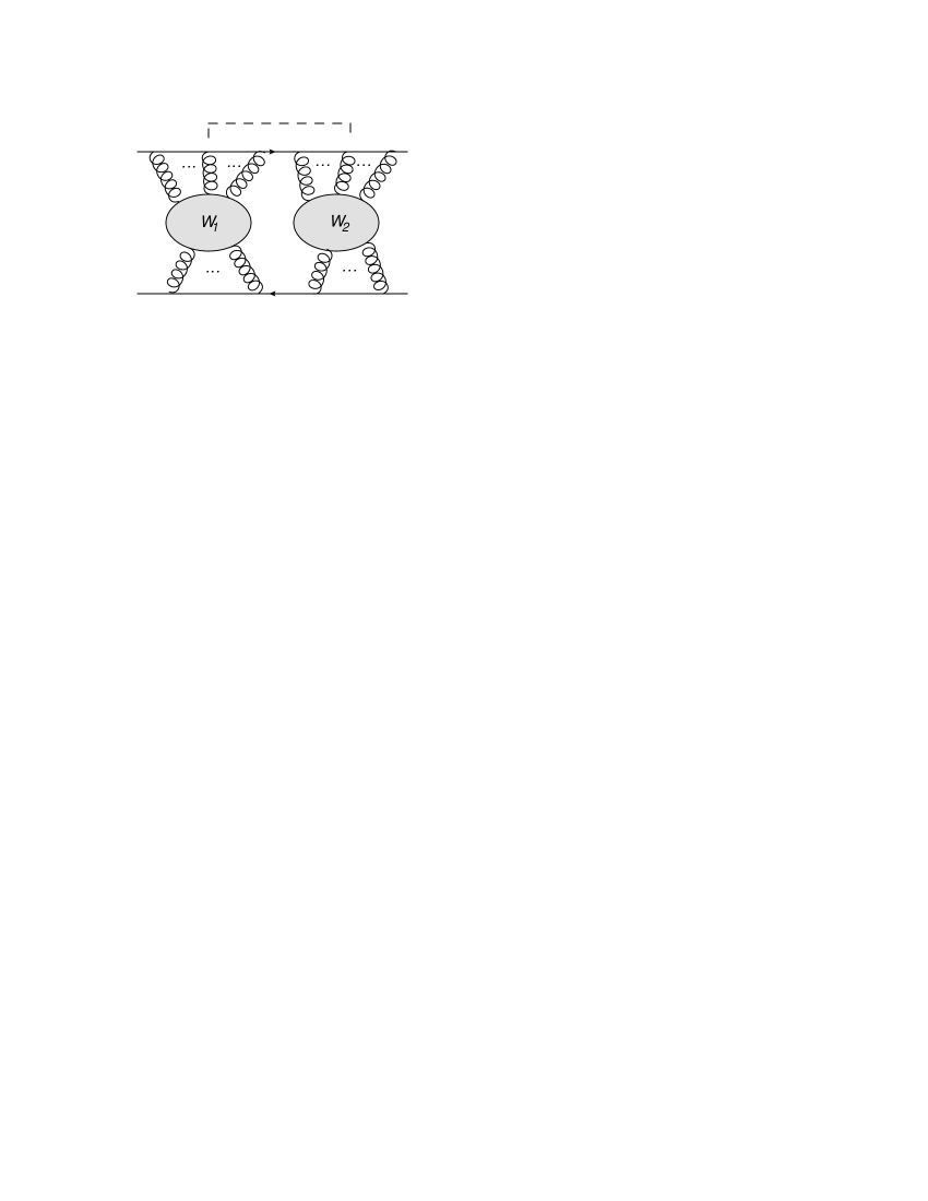
These diagrams are then two-eikonal-line irreducible, and thus must contribute to the exponent. Corresponding diagrams where the two-gluon vertex correlates gluons within one of the two webs are not present in the exponent, since they remain two-eikonal-line reducible. As a consequence, the contributions from all possible two-gluon vertex insertions no longer combine to form vertices depending on a single partial momentum sum, as they did above in the case of diagrams containing a single web. Instead, the leftover contributions form a remainder term, which has the same form as that discussed previously, in Sec. 3.4.

In more detail, consider again eq. (129), and assume for simplicity that the line being considered has contributions from two groups $g$ and $h$ only (the following discussion easily generalises to the case of more groups). Let us also take gluon $j$ as coming from group $g$. One may then split the sum on the left-hand side of eq. (129) into two parts, involving gluons from $g$ and $h$ respectively, to get

$${\cal C}_{{\rm NE},(1+2,j)}^{\mu_{1},\ldots,\mu_{m}}(n,k_{i})\,=\,\frac{1}{2n\cdot K_{j}}\left(g_{j}^{\mu_{j}}+2\sum_{i>j,\,i\in g}g_{i}^{\mu_{j}}+2\sum_{i>j,\,i\in h}h_{i}^{\mu_{j}}\right)\prod_{k\neq j}\left(-\frac{n^{\mu_{k}}}{n\cdot K_{k}}\right)\,,$$ (142)

where as usual $g_{i}$ is the momentum of the $i^{\text{th}}$ gluon from $g$. The first two terms in brackets combine to give the combination of partial momentum sums $G_{j}+G_{j+1}$, as already discussed in eq. (142), and lead to a next-to-eikonal emission vertex for gluon $j$ with eikonal Feynman rules for the remaining gluons. The second term can be rewritten as

$$\frac{H_{i}^{\mu_{j}}}{n\cdot(H_{i}+G_{j})}\prod_{k\neq j}\left(-\frac{n^{\mu_{k}}}{n\cdot K_{k}}\right)\,,$$ (143)

where $i$ labels the gluon from $h$ that is nearest (on the right-hand side) to the gluon from $g$. This has the form of a two-gluon correlation, with eikonal Feynman rules for the remaining gluons, and is the same as that given in eq. (84). Note that the previous result is expressed as a sum over all possible permutations of the gluons along the line, whereas here we consider only one such permutation. Also, we have yet to sum over the gluons $j$ from group $g$.

One may also consider eq. (140), again in the case in which two groups are present along the line. Considering the bracketed combination in the first line, all terms involving gluons from the same group combine to form a single squared partial momentum sum $G_{j}^{2}$ or $H_{j}^{2}$, as already discussed. There remain the terms in the double sum, in which the two gluons come from different groups. Considering the case where gluon $j$ comes from group $g$, the leftover terms are

$$2\sum_{l=j}^{m}\sum_{k>l}g_{l}\cdot h_{k}\,=\,2G_{j}\cdot H_{i}\,,$$ (144)

where again $i$ labels the gluon from $h$ that is nearest (on the right-hand side) to the gluon from $g$. Combining with the other factors in eq. (140), one has a contribution to the remainder term of

$$\frac{G_{j}\cdot H_{i}}{2n\cdot(G_{j}+H_{i})}\,\prod_{k}\left(-\frac{n^{\mu_{k}}}{n\cdot K_{i}}\right)\,.$$ (145)

After summing over all gluons from $g$, and all permutations of gluons on the line, this agrees with the result obtained in eq. (90). We have therefore demonstrated the full equivalence between the results of this paper and the path integral approach of Ref. [39].

The above discussion can be summarised as follows. In the diagrammatic approach of this paper, we find that contributions from different groups (derived from webs at eikonal and NE order containing local vertices only) factorise, up to a remainder term that correlates gluons between different groups. The NE Feynman rules thus obtained are precisely those that one finds through the path integral formalism, where the remainder term can be interpreted as correlating pairs of eikonal webs to form a new class of NE web. That the same structure and effective Feynman rules emerge from both the diagrammatic and path-integral viewpoints, is a highly non-trivial check of both approaches.

6 An illustrative example: the Drell-Yan process

In order to illustrate the results obtained in the previous sections, showing how they can be implemented in a concrete calculation, we consider in this section soft gluon corrections to the Drell-Yan production of a virtual photon in quark-antiquark annihilation. Since our focus here is just to give an example of the implementation of our NE rules, we will restrict our attention to abelian-like contributions to the cross section, which build up the $C_{F}^{p}$ color structure at $N^{p}LO$. Furthermore, we will consider only real radiation, since when including mixed real-virtual corrections we will need to account for Low’s theorem [41, 42, 43] contributions, which are not within the scope of the present paper. With these restrictions, we will compute soft gluon corrections up to NE level, and up to NNLO, using the rules developed in the previous sections. This is the simplest situation in which one can explicitly test NE exponentiation (as some of the two-loop NE corrections arise by expanding the exponential of the NE one-loop result). Furthermore, this calculation can be viewed as a preliminary step towards the generalisation of existing soft-gluon resummation methods to NLO in the threshold expansion, as well as a check of the validity of our analysis.

The NLO corrections to the Drell-Yan process were computed in [48], while the NNLO results was obtained in [49] (eikonal NNLO results were first presented in [50, 51]). We begin with a very brief summary of the LO calculation in order to introduce notation.

The LO Drell-Yan process [52], shown at parton level in fig. 15, proceeds through the channel

$${\cal Q}(p)+\bar{{\cal Q}}(\bar{p})\rightarrow\gamma^{*}(q^{\alpha})\,,$$ (146)

where ${\cal Q}$ denotes a quark, and $q^{\alpha}$ is the momentum of the off-shell photon.

Figure 15: Born level diagram for the Drell-Yan production of a an off-shell photon.

Since at higher orders (or at hadron level) the center-of-mass energy $s$ and the photon mass $Q^{2}=q^{2}$ do not coincide, it is customary to parametrize the Drell-Yan total cross section in terms of the variable $z=Q^{2}/s$, $0<z<1$. One then normalises the higher order cross-section to the Born result defining the $n$-loop $K$ factor $K^{(n)}(z)$ as

$$K^{(n)}(z)\,=\,\frac{1}{\sigma^{(0)}}\frac{d\sigma^{(n)}(z)}{dz}\,,$$ (147)

where $\sigma^{(n)}$ is the cross-section at ${\cal O}(\alpha_{s}^{n})$. The Born amplitude is simply

$${\cal M}_{(0)}^{\alpha}\,=\,\bar{u}(p)\gamma^{\alpha}v(\bar{p})\,,$$ (148)

where we drop coupling factors and spin averaging, as these will ultimately cancel upon taking ratios to compute the $K$ factor. Up to inessential factors, the Born cross section is given by

$$\sigma^{(0)} \propto -\int\frac{d^{d}q}{(2\pi)^{d-1}}\,(2\pi)^{n}\,\delta^{(n)}(q-p-\bar{p})\,\delta_{+}(q^{2}-Q^{2})\,\text{Tr}\left[{\not{p}}\gamma^{\alpha}\bar{\not{p}}\gamma_{\alpha}\right]$$ (149)

$$= 2\pi\delta_{+}(q^{2}-Q^{2})\,4p\cdot\bar{p}\,(d-2)\,,$$

where we will henceforth take $d=4-2\epsilon$. Clearly, the $K$ factor at leading order is simply given by

$$K^{(0)}(z)=\delta(1-z)\,.$$ (150)

We now move on to the NLO, next-to eikonal calculation.

6.1 Next-to-eikonal contributions at NLO

So far in this paper, we have only considered NE contributions to matrix elements. In calculating soft gluon contributions to cross-sections, one must also consider phase space integration. In the eikonal approximation (as is well known), the $n$-gluon phase space can be written as a product of decoupled one-gluon phase spaces. This is a necessary condition for the exponentiation of the cross-section which underlies soft-gluon resummations. At NE order the exact factorization of phase space breaks down, and it becomes necessary to study the unfactorized corrections to all orders. This is done, for the inclusive cross section, in Appendix B. Preliminarily, we note that at NE level one expects the schematic structure

$$\sigma_{\text{NE}}\,=\,\int\text{dPS}_{\text{eik}}\,|{\cal M}_{\text{NE}}|^{2}+\int\text{dPS}_{\text{NE}}|{\cal M}_{\text{eik}}|^{2}\,.$$ (151)

Here ${\cal M}_{\text{eik}}$ and ${\cal M}_{\text{NE}}$ are the eikonal and next-to-eikonal contributions to the matrix element, extensively discussed in the previous sections, and we have introduced an analogous expansion for the multi-gluon phase space measure of integration dPS. The NE correction to the phase space measure will also induce correlations between pairs of soft gluons, with a sum over all possible correlations. Up to NNLO, these corrections are easy to implement since the exact phase-space integration can be performed analytically, as we will do below.

We begin by computing the eikonal contributions to the NLO $K$-factor. Eikonal Feynman rules easily yield

$${\cal M}_{{\rm eik},\alpha}^{(1)}\left[{\cal M}_{\rm eik}^{(1)\,\alpha}\right]^{\dagger} = 2g_{s}^{2}C_{F}\,\frac{p\cdot\bar{p}}{(p\cdot k)(\bar{p}\cdot k)}\,\text{Tr}\left[{\not{p}}\gamma^{\alpha}\bar{\not{p}}\gamma_{\alpha}\right]$$ (152)

$$= 2g_{s}^{2}C_{F}\,\frac{8s^{2}}{ut}(1-\epsilon)\,.$$

where the factor of 2 in the first line comes from combining the two diagrams shown in fig. 16, and we have introduced the Mandelstam invariants

$$t=-2k\cdot p\,;\qquad u=-2k\cdot\bar{p}\,.$$ (153)

Figure 16: Squared matrix elements contributing at NLO in the eikonal limit. The cut denotes the final state.

To carry out the phase space integration, one may parametrise the four-vectors as

$$p=\frac{\sqrt{s}}{2}\left(1,1,{\bf 0}_{\perp}\right)\,;\quad\bar{p}=\frac{\sqrt{s}}{2}\left(1,-1,{\bf 0}_{\perp}\right)\,;\quad k=\frac{(1-z)\sqrt{s}}{2}\left(1,\cos\theta,\sin\theta,0\right)\,.$$ (154)

Defining then

$$y=\frac{1+\cos\theta}{2}\,,$$ (155)

one finds

$$t=-2s(1-y)(1-z)\,;\qquad u=-2sy(1-z)\,.$$ (156)

The NLO $K$-factor, defined in eq. (147), is computed by including a factor $\delta(k^{0}-(1-z)p^{0})$ in the two-particle phase space, and introducing the appropriate normalization, according to eq. (149). Setting the renormalization scale $\mu^{2}=Q^{2}$ one finds, at the eikonal level

$$K^{(1)}_{\rm eik}(z)\,=\,\frac{1}{16\pi^{2}}\,\frac{(4\pi)^{\epsilon}}{\Gamma(2-\epsilon)}\,z^{\epsilon}(1-z)^{1-2\epsilon}\int_{0}^{1}dy\,\big{[}y(1-y)\big{]}^{-\epsilon}{\cal M}_{{\rm eik},\alpha}^{(1)}\left[{\cal M}_{\rm eik}^{(1)\,\alpha}\right]^{\dagger}\,.$$ (157)

Substituting the squared eikonal matrix element given in eq. (152), performing the integration and Taylor expanding in $\epsilon$ this yields

$$K^{(1)}_{\rm eik}(z) = \frac{\alpha_{s}}{4\pi}\,C_{F}\,\Bigg{\{}-\frac{8}{\epsilon}{\cal D}_{0}(z)+16{\cal D}_{1}(z)-\frac{8\log(z)}{1-z}$$ (158)

$$-\,4\epsilon\left[4{\cal D}_{2}(z)-3\zeta_{2}{\cal D}_{0}(z)-\frac{4\log{z}\log(1-z)}{(1-z)}+\frac{\log^{2}z}{1-z}\right]\Bigg{\}}\,,$$

where, following [49], we use the notation

$${\cal D}_{p}(z)\,=\,\left[\frac{\log^{p}(1-z)}{1-z}\right]_{+}$$ (159)

to denote plus distributions. Note that we are not displaying terms proportional to $\delta(1-z)$, which mix with virtual contributions not considered here. Note also that eq. (158) contains terms that do not behave as $(1-z)^{-1}$: since we are using eikonal matrix elements, such terms arise from subleading corrections to the phase space measure.

Let’s now consider NE corrections to the matrix element. According to the results of Sec. 3, the effective Feynman rule for single gluon emission at NE order is

$$\frac{\gamma^{\mu}{\not{k}}}{2p\cdot k}-k^{2}\frac{p^{\mu}}{2(p\cdot k)^{2}}\,.$$ (160)

For real emission, the second term in eq. (160) vanishes since $k^{2}=0$. The diagrams contributing at NE level are shown in fig. 17, and consist of all possible insertions of at most one NE vertex in the eikonal diagrams of figure 16.

Figure 17: Diagrams contributing at NE level to the squared amplitude for NLO real emission. Two additional diagrams, arising from complex conjugation, are not shown.

The corresponding contribution to the squared matrix element is

$${\cal M}_{\text{NE},\alpha}^{(1)}\left[{\cal M}_{\rm eik}^{(1)\,\alpha}\right]^{\dagger}+{\cal M}_{{\rm eik},\alpha}^{(1)}\left[{\cal M}_{\text{NE}}^{(1)\,\alpha}\right]^{\dagger} = \frac{\bar{p}_{\mu}}{\bar{p}\cdot k}\frac{\text{Tr}\left[{\not{p}}\gamma^{\mu}{\not{k}}\gamma^{\alpha}\bar{\not{p}}\gamma_{\alpha}\right]}{2p\cdot k}+\frac{p_{\mu}}{p\cdot k}\frac{\text{Tr}\left[{\not{p}}\gamma^{\alpha}\bar{\not{p}}\gamma^{\mu}{\not{k}}\gamma_{\alpha}\right]}{2\bar{p}\cdot k}$$ (161)

$$= 8\,(1-\epsilon)\left(\frac{s}{t}+\frac{s}{u}\right).$$

Carrying out the phase space integration, dividing by the Born normalisation and expanding in $\epsilon$ leads to

$$K_{\text{NE}}^{(1)}(z) = \frac{\alpha_{s}}{4\pi}\,C_{F}\,\Bigg{\{}\frac{8}{\epsilon}-16\log(1-z)+8\log z$$ (162)

$$\quad-4\epsilon\left[-4\log^{2}(1-z)+4\log z\log(1-z)-\log^{2}z+3\zeta_{2}\right]\Bigg{\}}\,.$$

Combining eqs. (158) and (162) and retaining only terms with a logarithmic dependence on $z$, up to NE order, we obtain

$$K^{(1)}(z) = \frac{\alpha_{s}}{4\pi}\,C_{F}\,\Bigg{\{}-\frac{8}{\epsilon}{\cal D}_{0}(z)+16{\cal D}_{1}(z)-16\log(1-z)-4\epsilon\Big{[}4\,{\cal D}_{2}(z)-3\zeta_{2}{\cal D}_{0}(z)$$ (163)

$$\quad-4\log^{2}(1-z)+4\log(1-z)\Big{]}\Bigg{\}}\,.$$

Note that to obtain this result we expanded around $z=1$, including for example the replacement $\log z\to-(1-z)$.

One may compare this result with the corresponding exact NLO result including the complete $z$ dependence [48]. One easily verifies that expanding the exact result around $z=1$ gives eq. (163). Thus, the effective Feynman rules derived in the previous sections pass a first simple test.

6.2 Next-to-eikonal contributions at NNLO

In this section we compute the contribution proportional to $C_{F}^{2}$ to the NNLO $K$-factor for DY production of a virtual photon, and, as in the previous section, we restrict our attention to real gluon emission from a $q\bar{q}$ initial state. This is the simplest possible example illustrating the analysis performed in sections 2-4.

The structure of NE corrections found in the preceding sections implies that the amplitude for the double-real-emission graphs can be extracted, up to NE accuracy, from the expansion of an exponential with the schematic structure

$${\cal M}\,=\,{\cal M}^{(0)}\,\exp\left[\bar{\cal M}_{\rm eik}^{(1)}+\bar{\cal M}_{\text{NE}}^{(1)}+\bar{\cal M}_{\text{NE}}^{(2)}\right]\,,$$ (164)

where ${\cal M}^{(0)}\propto\text{Tr}\left[\not\!{p}\gamma^{\alpha}\not\!{\bar{p}}\gamma_{\alpha}\right]$, and the bar over an amplitude represents the expression for that amplitude with Born result factored out. Note there is no ${\cal O}(\alpha_{s}^{2})$ eikonal amplitude in the exponent. This is because we are considering only abelian graphs, and in that set there is no connected subdiagram involving two eikonal real emissions. In this language, the single and double real radiation matrix elements, up to NE accuracy, can be written as

$${\cal M}^{(1)} = {\cal M}^{(0)}\left[\bar{\cal M}_{\rm eik}^{(1)}+\bar{\cal M}_{\text{NE}}^{(1)}\right]\,,$$

$${\cal M}^{(2)} = {\cal M}^{(0)}\left[\frac{1}{2}\left(\bar{\cal M}_{\rm eik}^{(1)}\right)^{2}+\bar{\cal M}_{\rm eik}^{(1)}\bar{\cal M}_{\text{NE}}^{(1)}+\bar{\cal M}_{\text{NE}}^{(2)}\right]\,,$$ (165)

Since we are not considering virtual corrections, the only contributions to the squared matrix element that we will need at ${\cal O}(\alpha_{s}^{2})$ and at NE accuracy are given by

$${\cal M}^{(2)}\left[{\cal M}^{(2)}\right]^{\dagger} = \left|{\cal M}^{(0)}\right|^{2}\Bigg{\{}\left|\frac{1}{2}\left(\bar{\cal M}_{\rm eik}^{(1)}\right)^{2}\right|^{2}+2\,{\bf Re}\left[\frac{1}{2}\left(\bar{\cal M}_{\rm eik}^{(1)}\right)^{2}\left(\bar{\cal M}_{\rm eik}^{(1)}\bar{\cal M}_{\text{NE}}^{(1)}\right)^{\dagger}\right]$$ (166)

$$\qquad+\,2\,{\bf Re}\left[\frac{1}{2}\left(\bar{\cal M}_{\rm eik}^{(1)}\right)^{2}\left(\bar{\cal M}_{\text{NE}}^{(2)}\right)^{\dagger}\right]\Bigg{\}}$$

$$\equiv \left|{\cal M}^{(2)}\right|^{2}_{\rm eik}+\left|{\cal M}^{(2)}\right|^{2}_{\text{NE},{\rm 1g}}+\left|{\cal M}^{(2)}\right|^{2}_{\text{NE},{\rm 2g}}\,,$$

where, as the notation suggests, the first term is the eikonal approximation to the double real radiation matrix element squared, the second term is the NE correction arising from single-gluon NE vertices, and the third term is the NE correction arising from double-gluon NE vertices. We will treat each contribution in turn.

Let’s begin with the eikonal result, which has the explicit expression

$$\left|{\cal M}^{(2)}\right|^{2}_{\rm eik}\,=\,{\cal N}\,\frac{p\cdot\bar{p}}{p\cdot k_{1}\,p\cdot k_{2}\,\bar{p}\cdot k_{1}\,\bar{p}\cdot k_{2}}\,\text{Tr}\left[\not\!{p}\gamma^{\alpha}\not\!{\bar{p}}\gamma_{\alpha}\right]\,,$$ (167)

where, for simplicity, we have included in the normalization ${\cal N}$ all coupling, color and spin averaging factors, most of which drop out when constructing the $K$ factor.

The integration of eq. (167) over the three-body phase space is non-trivial, and we briefly discuss it here, since it will be needed also for the evaluaton of the NE corrections. We follow Ref. [49], and we evaluate the integrals in the center-of-mass frame of the two outgoing gluons. In order to perform the integral, we parametrise the momenta in $d=4-2\epsilon$ dimensions as in [49]. We write

$$k_{1} = \frac{\sqrt{s_{12}}}{2}\left(1,0,\ldots,\sin\theta_{2}\sin\theta_{1},\cos\theta_{2}\sin\theta_{1},\cos\theta_{1}\right)\,,$$

$$k_{2} = \frac{\sqrt{s_{12}}}{2}\left(1,0,\ldots,-\sin\theta_{2}\sin\theta_{1},-\cos\theta_{2}\sin\theta_{1},-\cos\theta_{1}\right)\,,$$

$$p = \frac{(s-\tilde{t})}{2\sqrt{s_{12}}}\left(1,0,\ldots,0,1\right)\,,$$ (168)

$$q = \left(\frac{s-Q^{2}-s_{12}}{2\sqrt{s_{12}}},0,\ldots,0,|\vec{q}|\sin\psi,|\vec{q}|\cos\psi\right)\,,$$

$$\bar{p} = \left(\frac{\tilde{t}+s_{12}-Q^{2}}{2\sqrt{s_{12}}},0,\ldots,0,|\vec{q}|\sin\psi,|\vec{q}|\cos\psi-\frac{(s-\tilde{t})}{2\sqrt{s_{12}}}\right)\,.$$

Here we have introduced the quantities

$$\tilde{t} \equiv 2p\cdot q\,=\,(p+q)^{2}-Q^{2}\,,$$

$$\tilde{u} = 2\bar{p}\cdot q\,=\,(\bar{p}+q)^{2}-Q^{2}\,,$$

$$s_{12} = 2k_{1}\cdot k_{2}\,=\,s-\tilde{t}-\tilde{u}+Q^{2}\,,$$ (169)

$$\cos\psi = \frac{(s-Q^{2})(\tilde{u}-Q^{2})-s_{12}(\tilde{t}+Q^{2})}{(s-\tilde{t})\sqrt{\lambda(s,Q^{2},s_{12})}}\,,$$

$$|\vec{q}| = \frac{\sqrt{\lambda(s,Q^{2},s_{12})}}{2\sqrt{s_{12}}}\,,$$

where $\lambda$ is the Källen function, $\lambda(a,b,c)=a^{2}+b^{2}+c^{2}-2ab-2ac-2bc$. The Mandelstam invariants $\tilde{t}$ and $\tilde{u}$ can in turn be expressed as functions of the photon energy fraction $z=Q^{2}/s$ and of two further variables $x$ and $y$, normalized so that $0<x<1$ and $0<y<1$, with the definitions

$$\tilde{u} = s\,\big{[}1-y(1-z)\big{]}\,,$$

$$\tilde{t} = s\left[z+y(1-z)-\frac{y(1-y)x(1-z)^{2}}{1-y(1-z)}\right]\,.$$ (170)

The $d$-dimensional three-body phase space can then be written as

$$\int\text{dPS}_{3} = \frac{1}{(4\pi)^{d}}\frac{s^{d-3}}{\Gamma(d-3)}(1-x)^{2d-5}\int_{0}^{\pi}d\theta_{1}\int_{0}^{\pi}d\theta_{2}\,(\sin\theta_{1})^{d-3}\,(\sin\theta_{2})^{d-4}$$ (171)

$$\,\times\,\int_{0}^{1}dy\int_{0}^{1}dx\big{[}y(1-y)\big{]}^{d-3}\big{[}x(1-x)\big{]}^{d/2-2}\big{[}1-y(1-z)\big{]}^{1-d/2}\,.$$

To integrate the matrix element squared in eq. (167) we still need expressions for the propagator factors in the current parametrization. They are

$$p\cdot k_{1} = \frac{s-\tilde{t}}{4}\,(1-\cos\theta_{1})\,$$

$$p\cdot k_{2} = \frac{s-\tilde{t}}{4}\,(1+\cos\theta_{1})\,$$ (172)

$$\bar{p}\cdot k_{1} = A-B\cos\theta_{1}-C\sin\theta_{1}\cos\theta_{2}$$

$$\bar{p}\cdot k_{2} = A+B\cos\theta_{1}+C\sin\theta_{1}\cos\theta_{2}\,,$$

where

$$A = \frac{\tilde{t}+s_{12}-Q^{2}}{4}\,,$$

$$B = \frac{\sqrt{s_{12}}}{2}\,|\vec{q}|\cos\psi-\frac{(s-\tilde{t})}{4}\,,$$ (173)

$$C = -\frac{\sqrt{s_{12}}}{2}\,|\vec{q}|\sin\psi\,.$$

It can be verified that $A^{2}=B^{2}+C^{2}$. Using this fact and putting together eq. (167) and eq. (171) one may verify that all the angular integrals to be performed can be reduced to the standard form

$$I^{(p,q)}_{d}(\chi) = \int_{0}^{\pi}d\theta_{1}\int_{0}^{\pi}d\theta_{2}\frac{\sin^{d-3}\theta_{1}\sin^{d-4}\theta_{2}}{(1-\cos\theta_{1})^{p}(1-\cos\chi\cos\theta_{1}-\sin\chi\sin\theta_{1}\cos\theta_{2})^{q}}$$

$$= 2^{1-p-q}\pi\,\frac{\Gamma(\frac{d}{2}-1-q)\Gamma(\frac{d}{2}-1-p)\Gamma(d-3)}{\Gamma(d-2-p-q)\Gamma^{2}(\frac{d}{2}-1)}\,\phantom{!}_{2}F_{1}\left[p,q;\frac{d}{2}-1;\cos^{2}\left(\frac{\chi}{2}\right)\right]\,,$$

where $\phantom{!}{}_{2}F_{1}$ is the standard hypergeometric function. Identifying $\cos\chi=-B/A$, using $\cos^{2}(\chi/2)=(1+\cos\chi)/2$, and expanding in powers of $\epsilon=2-d/2$, one gets, for example,

$$I_{4-2\epsilon}^{(1,1)}(\chi)\,=\,-\frac{\pi}{\epsilon}\left[\frac{A+B}{2A}\right]^{-1-\epsilon}\left\{1+\epsilon^{2}\,\text{Li}_{2}\left[\frac{A-B}{2A}\right]+{\cal O}\left(\epsilon^{3}\right)\right\}\,.$$ (175)

After performing the angular integrals in this way, the remaining integrations over $x$ and $y$ are easily carried out, after expanding the integrand in powers of $(1-z)$. This is consistent here since, for real emission contributions to the Drell-Yan cross section, the soft gluon expansion and the threshold expansion coincide. The resulting eikonal contribution to the NNLO $K$ factor reads

$$K^{(2)}_{\rm eik}(z) = \left(\frac{\alpha_{s}}{4\pi}\,C_{F}\right)^{2}\,\left[-\,\frac{32}{\epsilon^{3}}\,{\cal D}_{0}(z)+\frac{128}{\epsilon^{2}}\,{\cal D}_{1}(z)-\frac{256}{\epsilon}\,{\cal D}_{2}(z)-\frac{320}{\epsilon}\log(1-z)\right.$$ (176)

$$\qquad\left.+\,\frac{1024}{3}\,{\cal D}_{3}(z)+640\log^{2}(1-z)+\ldots\right]\,.$$

Note that for the sake of illustration we display only terms with a logarithmic dependence on $(1-z)$, and specifically those with rational coefficients, that are easily extracted from the exact calculation for comparison.

We now turn to NE corrections to the matrix element, and specifically we consider the second term in the last line of eq. (166), which arises from the insertion of single-gluon NE vertices. The application of the rules derived in the previous sections yields

$$\left|{\cal M}^{(2)}\right|^{2}_{\text{NE},{\rm 1g}}\,=\,-\,{\cal N}\,\left[\frac{s}{p\cdot k_{1}\,\bar{p}\cdot k_{1}}\left(\frac{1}{p\cdot k_{2}}+\frac{1}{\bar{p}\cdot k_{2}}\right)+\left(k_{1}\leftrightarrow k_{2}\right)\right]\,\text{Tr}\left[\not\!{p}\gamma^{\alpha}\not\!{\bar{p}}\gamma_{\alpha}\right]\,.$$ (177)

The integration over phase space can be carried out as for the eikonal term, and one finds a contribution to the $K$ factor given by

$$K^{(2)}_{\text{NE},{\rm 1g}}(z) = -\,\left(\frac{\alpha_{s}}{4\pi}\,C_{F}\right)^{2}\left[\frac{128}{\epsilon^{2}}\,\log(1-z)-\frac{256}{\epsilon}\,\log^{2}(1-z)\right.$$ (178)

$$\left.\qquad+\,\frac{1024}{3}\log^{3}(1-z)+\ldots\right]\,,$$

where again for simplicity we display only logarithmic terms with rational coefficients.

Finally, we need the contribution given by the final term in eq. (166), which involves NE contributions to two-gluon emission that don’t already arise from the exponentiation of the single emission. That is, one must include the contribution of the two-gluon vertices discussed in Sec. 3. The sum of the relevant vertices on, say, the quark line carrying momentum $p$ gives the tensor

$$R^{\mu\nu}(k_{1},k_{2};p)\,=\,-\,\frac{(p\cdot k_{2})p^{\mu}k_{1}^{\nu}+(p\cdot k_{1})k_{2}^{\mu}p^{\nu}-(p\cdot k_{1})(p\cdot k_{2})\,g^{\mu\nu}-(k_{1}\cdot k_{2})p^{\mu}p^{\nu}}{p\cdot(k_{1}+k_{2})}\,,$$ (179)

where an additional factor of two arises upon summing over the different orderings of the gluon momenta. Note that, given that this vertex joins two adjacent gluons, it includes the seagull vertex (i.e. the term in $g^{\mu\nu}$), as discussed in section 4.1. It is easily checked that this gives zero if either gluon lands on a fermion line carrying the same momentum $p$ as the emitter. Thus, the only possible contributions come from diagrams such as those shown in fig. 18.

Figure 18: Cut Feynman diagrams involving the next-to-eikonal two-gluon vertices summarized by the tensor $R^{\mu\nu}$. Note that also the complex conjugate diagrams must be included.

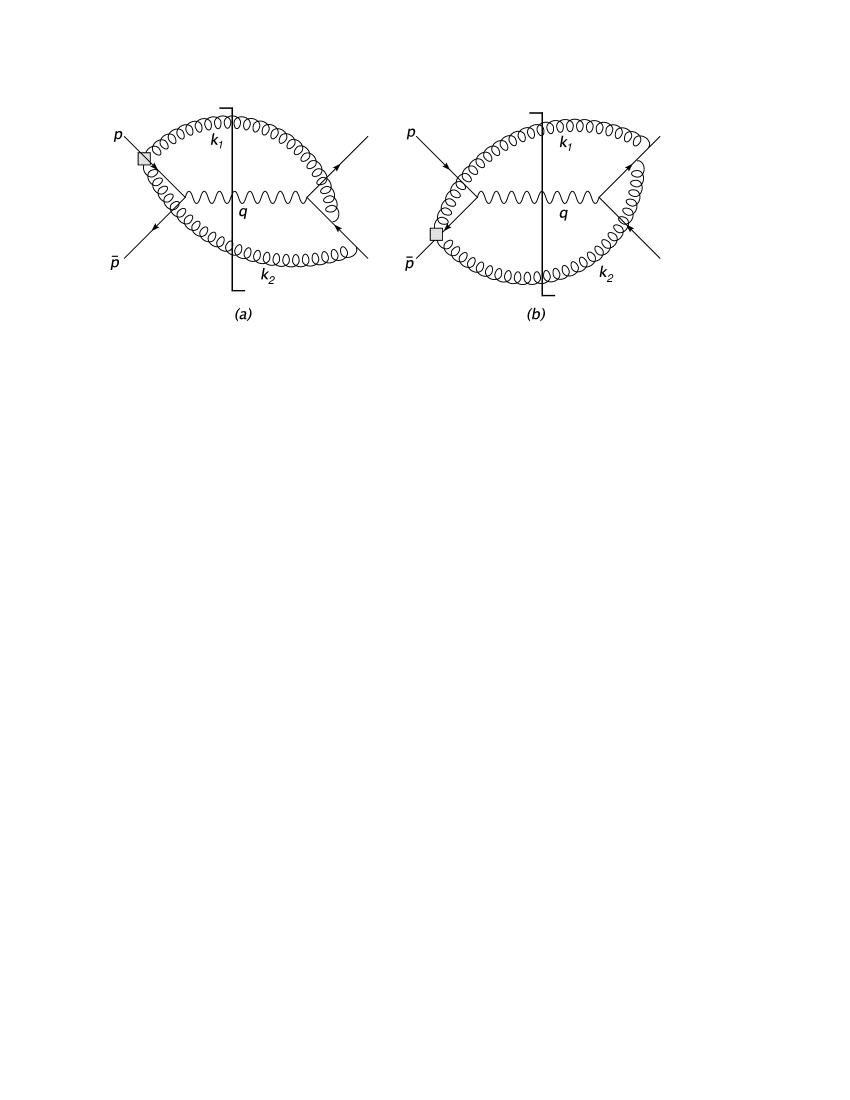
In fact, these diagrams also give a vanishing contribution, as can be seen from the following argument. Consider for example the diagram in fig. 18(a). This involves the factor

$$\frac{R^{\mu\nu}\bar{p}_{\mu}\bar{p}_{\nu}}{\bar{p}\cdot k_{1}\,\bar{p}\cdot k_{2}\,p\cdot k_{1}\,p\cdot k_{2}} = -\,\frac{p\cdot\bar{p}}{p\cdot(k_{1}+k_{2})\,\bar{p}\cdot k_{1}\,\bar{p}\cdot k_{2}\,p\cdot k_{1}\,p\cdot k_{2}}$$ (180)

$$\qquad\times\,\Big{[}p\cdot k_{2}\,\bar{p}\cdot k_{1}+\bar{p}\cdot k_{2}\,p\cdot k_{1}-k_{1}\cdot k_{2}\,p\cdot\bar{p}\Big{]}\,.$$

Note that the term in $R^{\mu\nu}$ involving $g_{\mu\nu}$ vanishes, since $\bar{p}^{2}=0$. If we now pick light-cone coordinates, such that $p^{\mu}=(p^{+},0^{-},{\bf 0}_{\perp})$ and $\bar{p}^{\mu}=(0^{+},\bar{p}^{-},{\bf 0}_{\perp})$, with $p^{\pm}\equiv(p^{0}\pm p^{3})/\sqrt{2}$, we observe that the factor in brackets on the r.h.s. of eq. (180) becomes

$$p\cdot k_{2}\,\bar{p}\cdot k_{1}+\bar{p}\cdot k_{2}\,p\cdot k_{1}-k_{1}\cdot k_{2}\,p\cdot\bar{p}\,=\,-\,\frac{s}{2}\,{\bf k}_{1,\perp}\cdot{\bf k}_{2,\perp}\,.$$ (181)

The prefactor of this term depends only on longitudinal momentum components. As a consequence, the diagram involving the two-gluon vertex gives a vanishing contribution upon integration over the gluon transverse momenta.

We conclude that the NE contribution to the NNLO $K$ factor is given just by the sum of eqs. (176) and (178). This, as expected, agrees with the result obtained from a full calculation of the double real emission contribution, followed by an expansion to NE order. The latter result is not available directly in the literature, but we include a short summary of the calculation in appendix C.

7 Conclusion

In this paper we have considered the exponentiation of soft gluon contributions to gauge theory amplitudes and cross sections, from a Feynman diagram viewpoint, classifying the structure of next-to-eikonal corrections. We showed that the notion of exponentiation can indeed be extended to NE order, as given by eq. (107). We note however that at NE level there are non-factorizable contributions which must be separately considered, and which are related to the radiationless amplitude by Low’s theorem and its generalizations. Factorizable contributions exponentiate and fall into two classes. First, there are conventional (eikonal) webs, modified by including effective NE Feyman rules; then, there are new webs formed by taking pairs of eikonal webs, and correlating a pair of gluons (one from each original web) with a two-gluon vertex. The derivation of this result relies upon establishing the appropriate generalisation of the eikonal identity, which is given in eq. (59) and expresses the fact that contributions from different groups factorise on a given external line, up to a remainder term which gives rise to the two-gluon vertex contributions mentioned above.

We performed a detailed comparison of the effective NE Feynman rules derived in this paper with the results obtained using the path integral formalism of [39], finding complete agreement between the two formalisms. This is a highly non-trivial cross-check of our classification of NE contributions to matrix elements, and also provides further insight on how to apply them in practice. In particular, a diagrammatic formalism makes contact with conventional factorization proofs, and is likely to be amenable to generalizations to hard collinear emissions which would be needed in order to perform a complete analysis of the threshold expansion beyond leading order.

The complete structure of next-to-eikonal corrections to QCD cross sections receives contributions not only from matrix elements but also from the integration over phase space for multiple soft-gluon emission. The discussion in this paper (see appendix B) shows how to treat these corrections for any number of gluons in the case of the Drell-Yan process; we expect that it should be possible to generalize these arguments to other processes.

Having classified the structure of NE corrections, it is interesting to ponder what might happen at NNE order (and beyond). Terms at this order in the expansion in gluon momenta are no longer divergent, but may nevertheless be numerically significant. The path-integral arguments of [39], as well as the recursive arguments presented in this paper, make clear that there is always a subset of external emission graphs which exponentiates at any given order in the momentum expansion. At higher orders, new vertices involving multiple gluon emissions will arise. More serious problems are bound to emerge, however, from non-factorizable contributions, which are governed by Low’s theorem at NE level. It is difficult to generalise the Low-Burnett-Kroll argument to higher orders in momentum, as gauge invariance does not then completely fix the structure of non-exponentiating contributions. Nevertheless, it might be the case that factorizable contributions dominate in practice, allowing for at least a partial resummation of NNE terms and beyond. It should also be noted that, as more finite orders terms are generated through exponentiation, it would become increasingly important to accurately match the resummed result to fixed-order perturbation theory, since a simple expansion of the exponential is bound to generate an increasing number of subleading terms which are beyond the accuracy guaranteed by resummation.

The results of this paper should be seen as a step towards the generalization of Sudakov resummation beyond leading order in the threshold expansion. In order to achieve the goal several further steps are still needed: the simple organization of phase space proposed in this paper must be brought to bear in a more formal way and in more general cross sections; non-factorizable contributions must be better understood; finally modifications of collinear evolution for hard collinear emissions must be fully understood at next-to-leading order in the threshold expansion. In order to show that our work is a step in the right direction, and as a first illustration of how to apply our effective Feynman rules at NE order, we reproduced a subset of NE logarithms in the real emission contribution to the Drell-Yan $K$-factor up to NNLO (specifically, those associated with the $C_{F}^{n}$ color structures). This is in a sense the simplest possible example, given that the limit $z\rightarrow 1$ for this process corresponds to soft singularities only, with no mixing from hard collinear divergences. One must also note that we have only discussed the simple case of a color-singlet hard interaction linking two partonic lines. We expect however that the bulk of our considerations will extend to more general color configurations, as indicated in  [13]. Work towards understanding these various generalizations is ongoing.

Acknowledgements

This research has been supported by the Foundation for Fundamental Research of Matter (FOM), as part of the programme TPP (Theoretical Particle Physics in the era of the LHC, FP 104); by the National Organization for Scientific Research (NWO); by MIUR (Italy) under contract 2006020509$\_$004; and by the European Community’s Marie-Curie Research Training Network ‘Tools and Precision Calculations for Physics Discoveries at Colliders’ (‘HEPTOOLS’), under contract MRTN-CT-2006-035505. CDW is supported by the STFC postdoctoral fellowship “Collider Physics at the LHC”, and thanks the Nikhef theory group for hospitality. LM thanks the CERN Theory Division for hospitality and support during crucial stages of this work.

Appendix A Rearranging NE numerators for spin-$\frac{1}{2}$ particles

We wish to prove that, when acting on a massless spinor, the following identity holds:

$$N^{\mu_{1}\ldots\mu_{n}} \equiv \sum_{i=1}^{n}\,\left[\prod_{j=i+1}^{n}\left(2p^{\mu_{j}}\right)\,\prod_{k=1}^{i-1}\left({\not{p}}\gamma^{\mu_{k}}\right)\,\gamma^{\mu_{i}}{\not{K}}_{i}\right]$$

$$= \sum_{i=1}^{n}\,\left[\prod_{j\neq i}\left(2p^{\mu_{j}}\right)\,\gamma^{\mu_{i}}{\not{k}}_{i}\,+\prod_{j\neq i,i-1}\left(2p^{\mu_{j}}\right)\,2p\cdot K_{i}\,\gamma^{\mu_{i-1}}\gamma^{\mu_{i}}\right]\,,$$

where we use $N^{\mu_{1}\ldots\mu_{n}}$ as a shorthand for $-{\cal N}_{\text{NE},2}^{\mu_{1}\ldots\mu_{n}}(p,k_{i})$, and where $K_{i}=\sum_{p=i}^{n}k_{p}$. Note that, as the notation suggests, the second term in the second line vanishes for $i=1$. We begin by observing that eq. (A) can easily be verified for low values of $n$, and indeed is trivial for $n=1$. This suggests setting up a recursive argument. In order to proceed, we first isolate the contribution of the first gluon in the l.h.s. of eq. (A), writing

$$N^{\mu_{1}\ldots\mu_{n}}\,=\,\prod_{j=2}^{n}\left(2p^{\mu_{j}}\right)\,\gamma^{\mu_{1}}{\not{K}}_{1}+\,{\not{p}}\gamma^{\mu_{1}}\,\sum_{i=2}^{n}\,\left[\prod_{j=i+1}^{n}\left(2p^{\mu_{j}}\right)\,\prod_{k=2}^{i-1}\left({\not{p}}\gamma^{\mu_{k}}\right)\,\gamma^{\mu_{i}}{\not{K}}_{i}\right]\,,$$ (183)

We can now use the induction hypothesis, assuming that eq. (A) holds for $n-1$ emissions, and using it to replace the sum in the second term of eq. (183). We get

$$N^{\mu_{1}\ldots\mu_{n}} = \prod_{j=2}^{n}\left(2p^{\mu_{j}}\right)\,\gamma^{\mu_{1}}{\not{K}}_{1}$$

$$+\,\,{\not{p}}\gamma^{\mu_{1}}\,\sum_{i=2}^{n}\,\left[\prod_{j\neq i}\left(2p^{\mu_{j}}\right)\,\gamma^{\mu_{i}}{\not{k}}_{i}\,+\prod_{j\neq i,i-1}\left(2p^{\mu_{j}}\right)\,2p\cdot K_{i}\,\gamma^{\mu_{i-1}}\gamma^{\mu_{i}}\right]\,.$$

Observe that the factor $(2p^{\mu_{1}})$ never appears on the second line, where the sum starts with the second emission, and for the same reason the last term starts contributing only for $i=3$. We now operate on the first term on the second line of eq. (A), using the commutation relation

$$\left[{\not{p}}\gamma^{\mu},\gamma^{\nu}{\not{k}}\right]\,=\,2\,p\cdot k\,\gamma^{\mu}\gamma^{\nu}-2\,p^{\nu}\,\gamma^{\mu}{\not{k}}$$ (185)

in order to bring the operator ${\not{p}}$ to the right of the expression, where it annihilates the massless spinor. We find

$$N^{\mu_{1}\ldots\mu_{n}} = \prod_{j=2}^{n}\left(2p^{\mu_{j}}\right)\,\gamma^{\mu_{1}}{\not{K}}_{1}+\sum_{i=2}^{n}\,\left[\prod_{j\neq i}\left(2p^{\mu_{j}}\right)\,\left(\gamma^{\mu_{i}}{\not{k}}_{i}\,{\not{p}}\gamma^{\mu_{1}}+2\,p\cdot k_{i}\gamma^{\mu_{1}}\gamma^{\mu_{i}}-\gamma^{\mu_{1}}{\not{k}}_{i}\,2p^{\mu_{i}}\right)\right]$$ (186)

$$+\,\,{\not{p}}\gamma^{\mu_{1}}\sum_{i=3}^{n}\left[\prod_{j\neq i,i-1}\left(2p^{\mu_{j}}\right)\,2\,p\cdot K_{i}\,\gamma^{\mu_{i-1}}\gamma^{\mu_{i}}\right]\,.$$

The last term in the sum on the first line has a factor $\prod_{j=2}^{n}\left(2p^{\mu_{j}}\right)$ for every value of the summation index $i$: one can then perform the sum getting simply a factor of ${\not{K}}_{2}$. This can be combined with the first term in eq. (186), using the fact that $K_{1}-K_{2}=k_{1}$. The result is simply $\prod_{j=2}^{n}\left(2p^{\mu_{j}}\right)\gamma^{\mu_{1}}{\not{k}}_{1}$. This can, in turn, be combined with the first term in the sum on the first line, where the factor of ${\not{p}}$ can be commuted across $\gamma^{\mu_{1}}$ to yield $2p^{\mu_{1}}$. One now has precisely all terms needed to reconstruct the sum of the first terms on the r.h.s. of eq. (A). One finds at this stage

$$N^{\mu_{1}\ldots\mu_{n}} = \sum_{i=1}^{n}\,\left[\prod_{j\neq i}\left(2p^{\mu_{j}}\right)\,\gamma^{\mu_{i}}{\not{k}}_{i}\right]+\sum_{i=2}^{n}\left[\prod_{j\neq i}\left(2p^{\mu_{j}}\right)\,2\,p\cdot k_{i}\gamma^{\mu_{1}}\gamma^{\mu_{i}}\right]$$ (187)

$$\,+\,\,{\not{p}}\gamma^{\mu_{1}}\sum_{i=3}^{n}\left[\prod_{j\neq i,i-1}\left(2p^{\mu_{j}}\right)\,2\,p\cdot K_{i}\,\gamma^{\mu_{i-1}}\gamma^{\mu_{i}}\right]\,.$$

Next, we act on the second line in eq. (187) applying the commutation relation

$$\left[{\not{p}}\gamma^{\rho},\gamma^{\mu}\gamma^{\nu}\right]\,=\,\gamma^{\rho}\gamma^{\mu}\,\,2\,p^{\nu}-\gamma^{\rho}\gamma^{\nu}\,\,2\,p^{\mu}\,,$$ (188)

also in order to bring the factor ${\not{p}}$ to act on the massless spinor to the right. This leads to

$$N^{\mu_{1}\ldots\mu_{n}} = \sum_{i=1}^{n}\,\left[\prod_{j\neq i}\left(2p^{\mu_{j}}\right)\,\gamma^{\mu_{i}}{\not{k}}_{i}\right]+\sum_{i=2}^{n}\left[\prod_{j\neq i}\left(2p^{\mu_{j}}\right)\,2\,p\cdot k_{i}\gamma^{\mu_{1}}\gamma^{\mu_{i}}\right]$$

$$+\,\sum_{i=3}^{n}\left[\prod_{j\neq i,i-1}\left(2p^{\mu_{j}}\right)\,2\,p\cdot K_{i}\,\Big{(}\gamma^{\mu_{i-1}}\gamma^{\mu_{i}}\,2\,p^{\mu_{1}}+\gamma^{\mu_{1}}\gamma^{\mu_{i-1}}\,2\,p^{\mu_{i}}-\gamma^{\mu_{1}}\gamma^{\mu_{i}}\,2\,p^{\mu_{i-1}}\Big{)}\right]\,.$$

At this stage, one just needs to properly recombine the terms in in the second and in the third sum in eq. (A) in order to recover eq. (A). We do this in the following way.

• Combining the term with $i=2$ in the second sum with the term $i=3$ for the second term of the third sum, and using the fact that $k_{2}+K_{3}=K_{2}$, one gets from these two terms a contribution

  $$\prod_{j\neq 2}\left(2p^{\mu_{j}}\right)\,2\,p\cdot K_{2}\,\gamma^{\mu_{1}}\gamma^{\mu_{2}}\,,$$ (190)

  which is the first non-vanishing contribution (the one with $i=2$) to the last term in eq. (A).

• One easily recognizes that all remaining terms in the last sum in eq. (A) are given precisely by the first term in the last sum in eq. (A), when the sum is performed in the range $3\leq i\leq n$), as written. Eq. (A) is thus already complete: it remains to be shown that the leftover terms in eq. (A) cancel.

• Consider indeed the remaining terms in the second sum in eq. (A) (those with $3\leq i\leq n$). Using the fact that $k_{i}-K_{i}=-K_{i+1}$, they can be combined with the third term of the third sum, which is summed over the same range, to get

  $$\sum_{i=3}^{n}\left[\prod_{j\neq i}\left(2p^{\mu_{j}}\right)\,\left(-2\,p\cdot K_{i+1}\right)\,\gamma^{\mu_{1}}\gamma^{\mu_{i}}\right]\,.$$ (191)

  It is easy to see that this sum precisely cancels the leftover contributions from second term in the last sum in eq. (A), which are in the range $4\leq i\leq n$, by just shifting $i+1\to i$ in eq. (191). This completes the proof of eq. (A).

Appendix B Next-to-eikonal phase space at arbitrary order

In the Sec. 6.2 we have illustrated the use of next-to-eikonal Feynman rules by calculating certain NNLO contributions to the Drell-Yan cross section. In order to correctly calculate logarithmic contributions which become dominant near partonic threshold, one must include corrections to the phase space measure of integration, as well as to matrix elements. We have seen that, at one and two loops, these corrections have a simple form and are easily taken into account. In order to perform a resummation, however, we will need to study NE corrections to the phase space measure to all orders in perturbation theory, that is for any number of emitted gluons. In this appendix we show, for the Drell-Yan process and for observables where the soft gluon phase space is integrated over, that the phase space measure remains very simple at NE order and for any number of emitted gluons. Indeed, it turns out to be possible to express this measure assigning identical factors to each emitted gluon, in a way that generalizes the known factorization properties of multi-gluon phase space at eikonal level. This will be instrumental in extending resummation techniques for physical cross sections to subleading orders in the threshold expansion.

Let us briefly recall the effects of subleading phase space corrections at one and two loops. In the case of one final state gluon (eq. (157)), dependence on the energy fraction $z$ factors out of the integration over the angular parameter $y$, and subleading corrections straightforwardly result upon expanding the $z$-dependent prefactor in powers of $\epsilon$. When two real gluon emissions are present, as in eq. (171), the integration measure contains the factor

$$\big{[}1-y\,(1-z)\big{]}^{-1+\epsilon}\,=\,1+\left(1-\epsilon\right)(1-z)+{\cal O}\left[(1-z)^{2}\right]\,.$$ (192)

Keeping only the first order term on the right-hand side corresponds to the NE approximation, which in the present case coincides with the next-to-leading order in the threshold expansion. We will now show how eq. (192) can be simply generalized to $n$-gluon emission.

Our starting point is the $(n+1)$-body phase space for the emission of $n$ gluons together with a final state vector boson. Using standard factorization properties, we write this as

$$\int\text{dPS}\left(p+\bar{p}\rightarrow q+k_{1}+\ldots k_{n}\right) = \int_{0}^{\infty}\frac{dK^{2}}{2\pi}\int\text{dPS}\left(p+\bar{p}\rightarrow q+K\right)$$ (193)

$$\quad\times\,\int\text{dPS}\left(K\rightarrow k_{1}+\ldots k_{n}\right)\,.$$

Here $\text{dPS}(A\to B)$ denotes the phase space for the reaction $A\to B$, $q$ is the 4-momentum of the vector boson and $\{k_{i}\}$ the momenta of the emitted gluons. On the right-hand side of eq. (193) we have introduced the vector sum of the emitted gluon momenta $K=\sum_{i=1}^{n}k_{i}$. One may interpret the product of phase spaces on the right-hand side of eq. (193) in terms of the production of a pseudo-particle of invariant mass $K^{2}$, followed by its decay into $n$ massless gluons; one then integrates over all possible invariant masses $K^{2}$. The convenience of this decomposition is that the two body phase space in eq. (193) is the same for any number of gluons, and depends upon the momenta of the latter solely through $K^{2}$. One may then evaluate the two-body phase space by parametrising momenta as

$$p = \frac{\sqrt{s}}{2}\left(1,0,\ldots,0,1\right)\,;$$

$$\bar{p} = \frac{\sqrt{s}}{2}\left(1,0,\ldots,0,-1\right)\,;$$ (194)

$$q = \left(\sqrt{|\vec{q}|^{2}+Q^{2}},0,\ldots,|\vec{q}|\sin\psi,|\vec{q}|\cos\psi\right)\,;$$

$$K = \left(\sqrt{|\vec{q}|^{2}+K^{2}},0,\ldots,-|\vec{q}|\sin\psi,-|\vec{q}|\cos\psi\right)\,.$$

Straightforward manipulations in $d=4-2\epsilon$ dimensions yield

$$\text{dPS}\left(p+\bar{p}\rightarrow q+K\right)\,=\,\frac{1}{8\pi\sqrt{s}}\,\frac{(4\pi)^{\epsilon}}{\Gamma(1-\epsilon)}\left(\frac{\lambda^{1/2}(Q^{2},K^{2},s)}{2\sqrt{s}}\right)^{1-2\epsilon}\left(\sin\psi\right)^{1-2\epsilon}\,d\psi\,,$$ (195)

where $\lambda(x,y,z)=x^{2}+y^{2}+z^{2}-2xz-2xy-2yz$ is the Källen function. As in the case of one real gluon emission (corresponding to $K^{2}=0$), one may define the Mandelstam invariants

$$t = -2K\cdot p\,=\,-\,\sqrt{s}\left(\sqrt{|\vec{q}|^{2}+Q^{2}}-|\vec{q}|\cos\psi\right)\,;$$

$$u = -2K\cdot\bar{p}\,=\,-\,\sqrt{s}\left(\sqrt{|\vec{q}|^{2}+Q^{2}}+|\vec{q}|\cos\psi\right)\,.$$ (196)

One may then show that

$$\sin^{2}\psi\,=\,\frac{4\left(tu-Q^{2}s\right)}{\lambda(Q^{2},K^{2},s)}\,,$$ (197)

so that the two-body phase space may be written as

$$\text{dPS}\left(p+\bar{p}\rightarrow q+K\right)\,=\,\frac{1}{8\pi}\,\frac{(4\pi)^{\epsilon}}{\Gamma(1-\epsilon)}\,s^{-1+\epsilon}\,\left(tu-Q^{2}s\right)^{1/2-\epsilon}d\psi\,.$$ (198)

The $n$-body phase space in eq. (193), on the other hand, is complicated in general. If however one performs all integrations for fixed total invariant mass $K^{2}$, the dependence of the result on $K^{2}$ is dictated by dimensional analysis, and is of the form

$$\int\text{dPS}\left(K\rightarrow k_{1}+\ldots k_{n}\right)\,=\,(K^{2})^{n-2-(n-1)\epsilon}\int\widehat{\text{dPS}}\left(K\rightarrow k_{1}+\ldots k_{n}\right)\,,$$ (199)

where $\widehat{\text{dPS}}$ on the right-hand side denotes a dimensionless bounded measure of integration depending only on the angles between the gluons in a chosen frame (for example their center of mass frame, as in Sec. 6.2). This measure is therefore independent of $K^{2}$, $Q^{2}$ and $z=Q^{2}/s$. Using the Jacobian

$$dK^{2}\,d\psi\,=\,\frac{1}{\sqrt{tu-Q^{2}s}}\,dt\,du\,,$$ (200)

the full phase space of eq. (193) becomes

$$\int\text{dPS}\left(p+\bar{p}\rightarrow q+k_{1}+\ldots k_{n}\right) = \frac{1}{16\pi^{2}}\,\frac{(4\pi)^{\epsilon}}{\Gamma(1-\epsilon)}\,s^{-1+\epsilon}\,\int dt\,du\,(K^{2})^{n-2-(n-1)\epsilon}$$ (201)

$$\times\,\left(tu-Q^{2}s\right)^{-\epsilon}\,\int\widehat{\text{dPS}}\left(K\rightarrow k_{1}+\ldots k_{n}\right)\,.$$

As in Sec. 6.2, it is convenient to introduce the variables $x$ and $y$ defined implicitly in terms of $u$ and $t$ as in eq. (170). The Jacobian is

$$du\,dt\,=\,\frac{y\,(1-y)}{1-y(1-z)}\,(1-z)^{3}\,s^{2}\,dx\,dy\,,$$ (202)

so that the full phase space takes the final form

$$\int\text{dPS}\left(p+\bar{p}\rightarrow q+k_{1}+\ldots k_{N}\right) = \frac{1}{16\pi^{2}}\frac{(4\pi)^{\epsilon}}{\Gamma(1-\epsilon)}\,s^{n-1-n\epsilon}(1-z)^{2n-1-2n\epsilon}$$

$$\times\int_{0}^{1}dy\int_{0}^{1}dx\,\big{[}y(1-y)\big{]}^{n-1-n\epsilon}\,x^{n-2-(n-1)\epsilon}\,(1-x)^{-\epsilon}$$

$$\times\,\big{[}1-y(1-z)\big{]}^{-(n-1)(1-\epsilon)}\int\widehat{\text{dPS}}\left(K\rightarrow k_{1}+\ldots k_{n}\right)\,.$$

One sees that the dependence on the energy fraction $z$ has only two sources: the overall prefactor of $(1-z)^{2n-1-2n\epsilon}$, which conspires with the matrix element to give the leading power $(1-z)^{-1}$ in the threshold expansion of the cross section, and the factor $[1-y(1-z)]^{-(n-1)(1-\epsilon)}$, which is neglected in the eikonal approximation. One observes that eq. (B), for $n=2$, reduces as expected to the three-particle phase space measure in eq. (171).

It is interesting to note that, at NLO in the threshold expansion, the $z$ dependence of the phase space measure in eq. (B) can be expressed in factorized form, with the same factor assigned to each emitted gluon. Indeed

$$\big{[}1-y(1-z)\big{]}^{-(n-1)(1-\epsilon)} = 1+(n-1)\,y\,(1-z)\left(1-\epsilon\right)+{\cal O}[(1-z)^{2}]\,$$ (204)

$$= z^{(1-\epsilon)\,y}\,\left(z^{-(1-\epsilon)\,y}\right)^{n}\,.$$

This provides, to some extent, a generalization of the factorization property of the multi-gluon phase space, which is known to degenerate into a product of uncorrelated single-gluon phase spaces at leading order in the threshold expansion. At NLO in the threshold expansion, the multi-gluon phase space measure is still factorizable, however the factors assigned to each emitted gluon retain a dependence on the angular variable $y$ describing the overall orientation on the multi-gluon system. In other words, single-gluon phase spaces are not fully uncorrelated, but their correlation is simple, depending only on the global variables of the multi-gluon system and not on individual gluon momenta.

This discussion applies to the explicit example of Drell-Yan production. We expect that such arguments will apply more generally in other scattering processes, pending a suitable parametrisation of the partonic momenta.

Appendix C The double-real-emission contribution to the Drell-Yan $K$ factor

In this appendix we briefly describe how to compute the terms proportional to $C_{F}^{2}$ of the Drell-Yan $K$-factor, for the $q\bar{q}$ initial state, by using ordinary Feynman diagrams and expanding them to NE order. The relevant diagrams are shown in fig. 19. The corresponding squared matrix elements are easily computed, and must then be integrated with the phase space measure in eq. (171).

Figure 19: Diagrams for the double-real-emission contribution to the NNLO Drell-Yan $K$ factor discussed in the text. A cut is implied over the intermediate state in each case, and complex conjugates of the above diagrams (excluding (e), which is real) must also be included.

As an example, diagram $(a)$ contributes a factor

$$|{\cal M}|^{2}_{(a)}\,\propto\,\frac{\text{Tr}\left[\not\!{\bar{p}}\gamma^{\alpha}(\not\!{p}-\not\!{k}_{1}-\not\!{k}_{2})\gamma^{\nu}(\not\!{p}-\not\!{k}_{1})\gamma^{\mu}\not\!{p}\gamma_{\alpha}(-\not\!{\bar{p}}+\not\!{k}_{1}+\not\!{k}_{2})\gamma_{\mu}(-\not\!{\bar{p}}+\not\!{k}_{2})\gamma_{\nu}\right]}{(p-k_{1}-k_{2})^{2}\,(p-k_{1})^{2}\,(-\bar{p}+k_{1}+k_{2})^{2}\,(-\bar{p}+k_{2})^{2}}\,.$$ (205)

Note that the contributions from diagrams $(a)-(d)$ must be counted twice in order to include Hermitian conjugate graphs, while diagram $(e)$ is real.

To calculate the squared matrix element to NE order, one first relabels $k_{i}\rightarrow\xi k_{i}$, so that

$$\bar{p}\cdot k_{i}\rightarrow\xi\,\bar{p}\cdot k_{i},\quad p\cdot k_{i}\rightarrow\xi\,p\cdot k_{i},\quad k_{i}\cdot k_{j}\rightarrow\xi^{2}\,k_{i}\cdot k_{j}\,.$$ (206)

One then expands each diagram to first subleading order in $\xi$, which corresponds to the NE approximation. Through repeated use of the identities

$$\frac{p\cdot k_{1}}{p\cdot k_{2}} = \frac{1}{p\cdot k_{2}}\frac{s-\tilde{t}}{2}-1\,,$$

$$\frac{\bar{p}\cdot k_{1}}{\bar{p}\cdot k_{2}} = \frac{1}{\bar{p}\cdot k_{2}}\frac{s_{12}+\tilde{t}-Q^{2}}{2}-1\,,$$ (207)

(with similar results for $k_{1}\leftrightarrow k_{2}$), each diagram can be written as a sum of terms containing no more than two factors of $p\cdot k_{i}$ and $\bar{p}\cdot k_{i}$. Then each term becomes an integral of the form of eq. (6.2). The remaining phase space integrals can be carried out after expanding the integrand in powers of $1-z$ and $\epsilon$, as described for the NE calculation in Sec. 6.2. The final result for the full amplitude (keeping only logarithmic terms with rational coefficients as done in the text) is given by

$$K^{(2)}_{\text{NE}}(z) = \left(\frac{\alpha_{s}}{4\pi}C_{F}\right)^{2}\left[-\frac{32}{\epsilon^{3}}\,{\cal D}_{0}(z)+\frac{128}{\epsilon^{2}}\,{\cal D}_{1}(z)-\frac{128}{\epsilon^{2}}\log(1-z)\right.$$ (208)

$$-\,\frac{256}{\epsilon}\,{\cal D}_{2}(z)+\frac{256}{\epsilon}\log^{2}(1-z)-\frac{320}{\epsilon}\log(1-z)$$

$$\left.+\,\frac{1024}{3}\,{\cal D}_{3}(z)-\frac{1024}{3}\log^{3}(1-z)+640\log^{2}(1-z)\right]\,,$$

which is in complete agreement with the sum of eqs. (176) and (178).

References

- [1] M. Levy and J. Sucher, Eikonal approximation in quantum field theory, Phys. Rev. 186 (1969) 1656.
- [2] H. D. I. Abarbanel and C. Itzykson, Relativistic eikonal expansion, Phys. Rev. Lett. 23 (1969) 53.
- [3] S. J. Wallace, Eikonal expansion, Annals Phys. 78 (1973) 190.
- [4] L. F. Alday and J. Maldacena, Lectures on scattering amplitudes via AdS/CFT, AIP Conf. Proc. 1031 (2008) 43.
- [5] E. Gardi and L. Magnea, Factorization constraints for soft anomalous dimensions in QCD scattering amplitudes, JHEP 03 (2009) 079, [0901.1091].
- [6] T. Becher and M. Neubert, On the Structure of Infrared Singularities of Gauge-Theory Amplitudes, JHEP 06 (2009) 081, [0903.1126].
- [7] T. Becher and M. Neubert, Infrared singularities of QCD amplitudes with massive partons, Phys. Rev. D79 (2009) 125004, [0904.1021].
- [8] E. Gardi and L. Magnea, Infrared singularities in QCD amplitudes, Nuovo Cim. C32N5-6 (2009) 137–157, [0908.3273].
- [9] D. R. Yennie, S. C. Frautschi, and H. Suura, The infrared divergence phenomena and high-energy processes, Ann. Phys. 13 (1961) 379.
- [10] G. Sterman, Infrared divergences in perturbative QCD, . in Tallahassee 1981, Proceedings, Perturbative Quantum Chromodynamics, 22-40.
- [11] J. G. M. Gatheral, Exponentiation of eikonal cross sections in nonabelian gauge theories, Phys. Lett. B133 (1983) 90.
- [12] J. Frenkel and J. C. Taylor, Nonabelian eikonal exponentiation, Nucl. Phys. B246 (1984) 231.
- [13] E. Gardi, E. Laenen, G. Stavenga, and C. D. White, Webs in multiparton scattering using the replica trick, 1008.0098.
- [14] A. Mitov, G. Sterman, and I. Sung, Diagrammatic exponentiation for products of Wilson lines, 1008.0099.
- [15] G. Sterman, Summation of large corrections to short-distance hadronic cross sections, Nucl. Phys. B281 (1987) 310.
- [16] S. Catani and L. Trentadue, Resummation of the QCD Perturbative series for hard processes, Nucl. Phys. B327 (1989) 323.
- [17] G. P. Korchemsky and G. Marchesini, Resummation of large infrared corrections using Wilson loops, Phys. Lett. B313 (1993) 433.
- [18] H. Contopanagos, E. Laenen, and G. Sterman, Sudakov factorization and resummation, Nucl. Phys. B484 (1997) 303, [hep-ph/9604313].
- [19] S. Forte and G. Ridolfi, Renormalization group approach to soft gluon resummation, Nucl. Phys. B650 (2003) 229, [hep-ph/0209154].
- [20] R. J. Hill, T. Becher, S. J. Lee, and M. Neubert, Sudakov resummation for subleading SCET currents and heavy-to-light form factors, JHEP 07 (2004) 081, [hep-ph/0404217].
- [21] T. Becher and M. Neubert, Threshold resummation in momentum space from effective field theory, Phys. Rev. Lett. 97 (2006) 082001, [hep-ph/0605050].
- [22] E. Gardi and G. Grunberg, A dispersive approach to Sudakov resummation, Nucl. Phys. B794 (2008) 61, [0709.2877].
- [23] M. D. Schwartz, Resummation and NLO Matching of Event Shapes with Effective Field Theory, Phys. Rev. D77 (2008) 014026, [0709.2709].
- [24] C. W. Bauer, S. P. Fleming, C. Lee, and G. F. Sterman, Factorization of e+e- Event Shape Distributions with Hadronic Final States in Soft Collinear Effective Theory, Phys. Rev. D78 (2008) 034027, [0801.4569].
- [25] J.-y. Chiu, A. Fuhrer, R. Kelley, and A. V. Manohar, Factorization Structure of Gauge Theory Amplitudes and Application to Hard Scattering Processes at the LHC, Phys. Rev. D80 (2009) 094013, [0909.0012].
- [26] M. Kramer, 1, E. Laenen, and M. Spira, Soft gluon radiation in Higgs boson production at the LHC, Nucl. Phys. B511 (1998) 523–549, [hep-ph/9611272].
- [27] T. O. Eynck, E. Laenen, and L. Magnea, Exponentiation of the Drell-Yan cross section near partonic threshold in the DIS and MS-bar schemes, JHEP 06 (2003) 057, [hep-ph/0305179].
- [28] S. Friot and G. Grunberg, Constant terms in threshold resummation and the quark form factor, JHEP 09 (2007) 002, [0706.1206].
- [29] V. Ahrens, T. Becher, M. Neubert, and L. L. Yang, Origin of the large perturbative corrections to Higgs production at hadron colliders, Phys. Rev. D79 (2009) 033013, [0808.3008].
- [30] Y. L. Dokshitzer, G. Marchesini, and G. P. Salam, Revisiting parton evolution and the large- limit, Phys. Lett. B634 (2006) 504, [hep-ph/0511302].
- [31] E. Laenen, L. Magnea, and G. Stavenga, On next-to-eikonal corrections to threshold resummation for the Drell-Yan and DIS cross sections, Phys. Lett. B669 (2008) 173, [0807.4412].
- [32] S. Moch and A. Vogt, On non-singlet physical evolution kernels and large-x coefficient functions in perturbative QCD, JHEP 11 (2009) 099, [0909.2124].
- [33] G. Soar, S. Moch, J. A. M. Vermaseren, and A. Vogt, On Higgs-exchange DIS, physical evolution kernels and fourth-order splitting functions at large x, Nucl. Phys. B832 (2010) 152, [0912.0369].
- [34] A. Vogt, G. Soar, S. Moch, and J. Vermaseren, On higher-order flavour-singlet splitting and coefficient functions at large x, 1008.0952.
- [35] A. Vogt, S. Moch, G. Soar, and J. A. M. Vermaseren, Higher-order predictions from physical evolution kernels, PoS RADCOR2009 (2010) 053, [1001.3554].
- [36] G. Grunberg and V. Ravindran, On threshold resummation beyond leading order, JHEP 10 (2009) 055, [0902.2702].
- [37] G. Grunberg, Large- structure of physical evolution kernels in Deep Inelastic Scattering, 0911.4471.
- [38] G. Grunberg, Threshold resummation beyond leading eikonal level, 1005.5684.
- [39] E. Laenen, G. Stavenga, and C. D. White, Path integral approach to eikonal and next-to-eikonal exponentiation, JHEP 03 (2009) 054, [0811.2067].
- [40] E. Laenen, L. Magnea, G. Stavenga, and C. D. White, On next-to-eikonal exponentiation, 1007.0624.
- [41] F. E. Low, Bremsstrahlung of very low-energy quanta in elementary particle collisions, Phys. Rev. 110 (1958) 974.
- [42] T. H. Burnett and N. M. Kroll, Extension of the low soft photon theorem, Phys. Rev. Lett. 20 (1968) 86.
- [43] V. Del Duca, High-energy bremsstrahlung theorems for soft photons, Nucl. Phys. B345 (1990) 369.
- [44] C. F. Berger, Soft gluon exponentiation and resummation, hep-ph/0305076. PhD Thesis.
- [45] S. Weinzierl, Introduction to Feynman integrals, 1005.1855.
- [46] M. J. Strassler, Field theory without Feynman diagrams: one-loop effective actions, Nucl. Phys. B385 (1992) 145, [hep-ph/9205205].
- [47] J. W. van Holten, Propagators and path integrals, Nucl. Phys. B457 (1995) 375, [hep-th/9508136].
- [48] G. Altarelli, R. K. Ellis, and G. Martinelli, Large perturbative corrections to the Drell-Yan process in QCD, Nucl. Phys. B157 (1979) 461.
- [49] R. Hamberg, W. L. van Neerven, and T. Matsuura, A Complete calculation of the order correction to the Drell-Yan factor, Nucl. Phys. B359 (1991) 343.
- [50] T. Matsuura, S. C. van der Marck, and W. L. van Neerven, The calculation of the second order soft and virtual contributions to the Drell-Yan cross section, Nucl. Phys. B319 (1989) 570.
- [51] T. Matsuura, S. C. van der Marck, and W. L. van Neerven, The order contribution to the factor of the Drell-Yan process, Phys. Lett. B211 (1988) 171.
- [52] S. D. Drell and T.-M. Yan, Massive lepton pair production in hadron-hadron collisions at high-energies, Phys. Rev. Lett. 25 (1970) 316–320.