Jet Reconstruction in Heavy Ion Collisions

Abstract

We examine the problem of jet reconstruction at heavy-ion colliders using jet-area-based background subtraction tools as provided by FastJet. We use Monte Carlo simulations with and without quenching to study the performance of several jet algorithms, including the option of filtering, under conditions corresponding to RHIC and LHC collisions. We find that most standard algorithms perform well, though the anti-$k_{t}$ and filtered Cambridge/Aachen algorithms have clear advantages in terms of the reconstructed $p_{t}$ offset and dispersion.

1 Introduction

Since the appearance of the first high-energy colliders in the 1980’s, the study of “jets” of particles produced in the final state has proved to be a powerful tool for probing the underlying elementary dynamics of the strong force as described by Quantum Chromodynamics (QCD). Jets have been extensively studied at $e^{+}e^{-}$ (LEP, SLC), $ep$ (HERA) and $p\bar{p}$/$pp$ (Tevatron, RHIC, LHC) colliders, with a wide variety of jet algorithms, including infrared and collinear (IRC) safe algorithms such as those of refs. [1, 2, 3, 4].

A topic of current interest is the use of jets in heavy-ion (HI) collisions, where, for example, they can be used to probe the hot, dense medium. In the past few years, the Relativistic Heavy Ion Collider (RHIC) has amassed significant numbers of copper-copper and gold-gold collisions at nucleon-nucleon centre of mass energies up to $\sqrt{s_{NN}}=200\,\mathrm{GeV}$, and the Large Hadron Collider (LHC) should deliver high yields of lead-lead collisions at much higher energies in the near future.

The main obstacle to studying jets in HI collisions is the presence of the huge background given by the underlying event (UE) produced simultaneously with the hard nucleon-nucleon collision that initiates the high-transverse momentum jet of interest. This UE needs to be properly subtracted from the momentum of a given jet in order to reconstruct its “true” momentum, i.e. the one it would have in the absence of the UE contribution. This problem is of course well known, and is also present, though to a much smaller extent, in jet studies in proton-proton collisions. Various approaches to address it have been proposed (see e.g. [5, 6, 7, 8, 9, 10, 11, 12, 13]).

In ref. [14] two of us proposed a jet area-related technique to determine the transverse momentum density of a sufficiently uniformly distributed background and to subtract it from the jet momenta. The method of [14] introduced several novel steps, such as the measurement of jet areas, and procedures to determine the transverse-momentum density of the underlying event and/or pileup. Subsequent work of ours [15, 16] has sought to provide firmer foundations for these concepts and methods, as well as practical tests in $pp$ jet reconstruction tasks with simulated events [17]. Preliminary experimental jet measurements from the STAR collaboration at RHIC, whose analysis is partially based on the ideas of [14], have been presented in ref. [18].

In this article we give a systematic examination of the performance of such methods for heavy-ion collisions, applying them to Monte Carlo simulations for RHIC and the LHC. In particular, we determine the accuracy with which jet momenta can be effectively reconstructed, comparing the performance of several different jet algorithms.

2 Challenges of jet reconstruction in heavy-ion collisions

Jets in HI collisions are produced in an environment that is far from conducive to their detection and accurate measurement. Monte Carlo simulations (and real RHIC data) for gold-gold collisions at $\sqrt{s_{NN}}=200$ GeV (per nucleon-nucleon collision) show that the transverse momentum density $\rho$ of final-state particles is about 100 GeV per unit area (in the rapidity-azimuth plane). For lead-lead collisions at $\sqrt{s_{NN}}=5.5$ TeV at the LHC this figure is expected to increase by some factor $\sim 2-3$. This means that jets returned by jet definitions with a radius parameter of, e.g., $R=0.4$, will contain background contamination of the order of $\pi R^{2}\rho\simeq$ 50 and $100-150\,\mathrm{GeV}$ respectively.

A related, and perhaps more challenging obstacle to accurate jet reconstruction is due to the fluctuations both of the background level (from event to event, but also from point to point in a single event) and of the jet area itself: knowing the contamination level ‘on average’ is not sufficient to accurately reconstruct each individual jet.

A wide range of strategies have already been advocated to reconstruct jets in HI collisions. Just to mention them briefly, approaches to HI jet reconstruction may involve one or more of the following measures: choosing a jet algorithm returning jets with an area as constant as possible; eliminating from the clustering all particles below a given transverse momentum threshold, say $p_{t,\min}\sim 2$ GeV; measuring the background level in a region of the detector thought to be not affected by the hard event; or parametrising the average background level (and fluctuations) in terms of some other measured properties of the event, such as its centrality.

Our framework has the following characteristics:

• We shall restrict ourselves to IRC safe jet algorithms, to ensure that measurements can be meaningfully compared to higher-order perturbative QCD calculations.

• The jet algorithms we use will not be limited to those yielding jets of regular shape.

• Our analysis will avoid excluding small transverse momentum particles from the clustering. Doing so is collinear-unsafe and inevitably biases the reconstructed jet momenta, which must then be corrected using Monte Carlo simulations, which can have substantial uncertainties in their modelling of jet quenching and energy loss. Instead, we shall try to achieve a bias-free reconstructed jet, working with all the particles in the event.

• The background level will be determined through adaptations of the jet-area/median procedure suggested in [14] and analysed in detail in [16]. This procedure is designed to give an estimate of the background that is minimally affected by the presence of hard jets.

3 Simulation and analysis framework

3.1 Hard and full events

In order to test the effectiveness of subtracting the underlying event in a heavy-ion collision, and determine the quality of the jet reconstruction, we need access to the idealised hard jets, without the background, as a reference. This can be done by considering a simulated hard $pp$ event first in isolation, and then embedded in a heavy-ion event. For clarity in the discussions, we shall adopt the following terminology:

• the hard event refers to the hard $pp$ event alone, without a heavy-ion background;

• the full event refers to combination of the hard event and the HI background (which possibly includes many semi-hard events of its own);

• hard jets and full jets refers to jets from the hard and full events, respectively.

Note that though making the distinction between a hard and a full event is not possible with real data, it is feasible in certain Monte Carlo studies. One should nevertheless be aware that the extent to which such a distinction is physically meaningful is a question that remains open in view of the numerous issues related to the interaction between an energetic parton and the medium through which it travels.

If the Monte Carlo program used to simulate heavy-ion events explicitly provides a separation between hard events and a soft part — e.g. as does HYDJET [19, 20] — one can extract one of the former as the single hard event and take the complete event as the full one. Alternatively, one can generate a hard event independently and embed it in a heavy-ion event (obtained from a Monte Carlo or from real collisions) to obtain the full event. This second approach, which we have adopted for the bulk of results presented here because of its greater computational efficiency, is sensible as long as the embedded hard event is much harder than any of the semi-hard events that tend to be present in the background. For the transverse momenta that we consider, this condition is typically fulfilled. Note however that for studies in which the presence of a hard collision is not guaranteed, e.g. the evaluation of fake-jet rates, one should use the first approach.

3.2 Matching and quality measures

To measure the performance of our heavy-ion background subtraction procedure we apply it to both hard and full events. We then take the two hardest resulting jets in each hard event and compare them to the corresponding subtracted jets in the full event.

To do this in practice, we need a method to match the jets obtained from the full event to those from the hard event alone, to make sure that we are comparing the same object. In other analyses, this matching was typically performed in terms of the position of the jet in the rapidity-azimuth plane, requiring that the two jet axes not differ by more than a given $\Delta R\equiv\sqrt{\Delta y^{2}+\Delta\phi^{2}}$. The exact value of $\Delta R$ is an arbitrary choice, and values between 0.1 and 0.3 have been often used. In order to avoid the arbitrariness of the $\Delta R$ choice, we propose a different prescription: a jet reconstructed in the full event is considered matched to a hard jet if the constituents common to both the hard and the full jet make up at least 50% of the transverse momentum of the constituents of the hard jet. This definition has the advantage that for a given hard jet, at most one full jet can satisfy this criterion, therefore avoiding having to deal with multiple positive matchings. Another advantage is that it automatically rejects fake matchings given by a soft jet that happens to be close to a hard one.

For a matched pair of jets, we shall use the notation $p_{t}^{pp}$ and $p_{t}^{AA}$ for the transverse momentum of the jet in the hard and full event respectively, and $p_{t}^{pp,{\rm sub}}$ and $p_{t}^{AA,{\rm sub}}$ for their subtracted equivalents. The quantity that we shall mostly concentrate on is the $p_{t}$ offset,

$$\Delta p_{t}\equiv p_{t}^{AA,{\rm sub}}-p_{t}^{pp,{\rm sub}}\,,$$ (1)

between the momentum of the background-subtracted jet in the full event and its equivalent in the hard event. Large deviations from zero will indicate a poor subtraction. Events without any matched jets are simply discarded and instead contribute to the evaluation of matching inefficiencies (see section 4.1).

The average of the $p_{t}$ shift over many events, $\langle\Delta p_{t}\rangle$, is only one measure that one may examine to establish the quality of jet reconstruction; its dispersion,

$$\sigma_{\Delta p_{t}}\equiv\sqrt{\left\langle\Delta p_{t}^{2}\right\rangle-\left\langle\Delta p_{t}\right\rangle^{2}}\,,$$ (2)

can be another important one. This is especially true in the case of steeply-falling jet spectra, where this dispersion can have a large impact on the measured cross section, necessitating delicate deconvolutions, also known as “unfolding”.

In this paper we shall concentrate on these two quality measures $\left\langle\Delta p_{t}\right\rangle$ and $\sigma_{\Delta p_{t}}$, keeping only the pair of jets that have been matched to one of the two hardest (subtracted) jets in the hard event. Small (absolute) values of both $\left\langle\Delta p_{t}\right\rangle$ and $\sigma_{\Delta p_{t}}$ will be the sign of a good subtraction. In practice a trade-off may exist in offset versus dispersion: which one to optimise may depend on the specific observable one wants to measure.

3.3 Monte Carlo simulations

Quantifying the quality of background subtraction using Monte Carlo simulations has several advantages. Besides providing a practical way of generating the hard “signal” separately from the soft background, one can easily check the robustness of one’s conclusions by changing the hard jet or the background sample.

One difficulty that arises in gauging the quality of jet reconstruction in heavy-ion collisions comes from the expectation that parton fragmentation in a hot medium will differ from that in a vacuum. This difference is often referred to as jet quenching [21] (for reviews, see [22]). The details of jet quenching are far less well established than those of vacuum fragmentation and can have an effect on the quality of jet reconstruction. Here we shall examine the reconstruction of both unquenched and quenched jets. For the latter it will be particularly important to be able to test more than one quenching model, in order to help build confidence in our conclusions about any reconstruction bias that may additionally exist in the presence of quenching.

In practice, for this paper we have used both the Fortran (v1.6) [19] and the C++ (v2.1) [20] versions of HYDJET to generate the background. Hard jets have been generated with PYTHIA 6.4 [23], either running it standalone, or using the version embedded in HYDJET v1.6. The quenching effects have been studied using both QPYTHIA [24] and PYQUEN [19].

3.4 Jet definitions

As mentioned in the Introduction, the last few years have seen many developments in the field of jet clustering, with the appearance of fast implementations [25] of the $k_{t}$ [1] and the Cambridge/Aachen [2] sequential recombination algorithms, and the introduction of the SISCone [4] and anti-$k_{t}$ [3] algorithms.

Besides these four main infrared-and-collinear-safe jet algorithms, a number of recent papers (see e.g. [26, 17]), have introduced and studied jet-cleaning techniques in order to help the reconstruction of jets by reducing the UE contamination. “Filtering” [26] works by reclustering each jet with a radius $R_{\rm filt}$ smaller than the original radius $R$ and keeping only the $n_{\rm filt}$ hardest subjets (background subtraction is applied to each of the subjets before deciding which ones to keep). Other similar techniques, “trimming” and “pruning”, that exploit the substructure of jets have also been introduced recently [27, 28] and, in $pp$ environments, have been found to give benefits comparable to those of filtering. Note that the filtering that we use here is unrelated to the Gaussian filter approach of [9] (not used in this paper as no public code is currently available).

In analogy with the systematic analysis of the performance of various jet definitions in the kinematic reconstruction of dijet systems at the LHC [17], here we will study how different algorithms behave in the case of HI collisions. We will use the $k_{t}$, Cambridge/Aachen (C/A), and anti-$k_{t}$ algorithms, as well as filtering applied to Cambridge/Aachen (C/A(filt)) with $R_{\rm filt}=R/2$ and $n_{\rm filt}=2$. We have not used SISCone, as its relatively slower speed compared to the sequential recombination algorithms makes it less suitable for a HI environment.

All the algorithms have been used through their fast implementation available in the FastJet package [25, 29], version 2.4.2. Additionally some features of a forthcoming FastJet release have been used to help simplify our analyses.

3.5 Background determination and subtraction

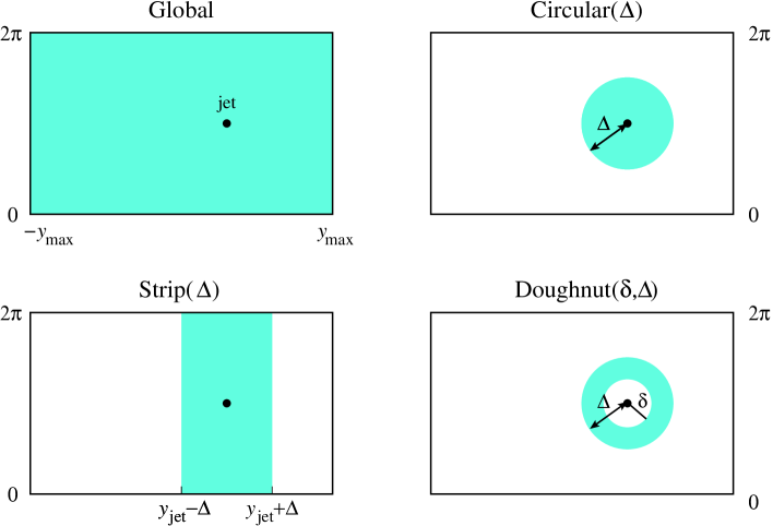
Figure 1: Graphical representation of the 4 different background-estimation ranges we shall consider: the Global range, the Strip range ${\cal S}_{\Delta}(j)$, the Circular range ${\cal C}_{\Delta}(j)$ and the Doughnut range ${\cal D}_{\delta,\Delta}(j)$. The last three are local ranges with a position depending on the jet being subtracted. See the text for detailed definitions.

In order to subtract the HI background from the hard jets, we will mainly follow the method introduced in [14]. When clustering the event we determine the 4-vector active area $A_{j}^{\mu}$ [15] of each jet $j$, as well as an estimate of the background density $\rho$. Then for each jet $j$, we subtract from its four-momentum the expected background contamination:

$$p_{j}^{\mu,{\rm sub}}=p_{j}^{\mu}-\rho A_{j}^{\mu}\,.$$ (3)

The background transverse-momentum density per unit area, $\rho$, is determined, event-by-event, as proposed in [14]. In that paper two ways of determining $\rho$ were explored. One was to take a global background-estimation range ${\cal R}$, covering the full rapidity-azimuth plane up to some rapidity $y_{\max}$; one then considered the set of ratios of transverse components of the momentum and area 4-vectors, $p_{j,t}/A_{j,t}$, for the jets within this range. The median of this set was used as an estimate for $\rho$:

$$\rho_{{\cal R}}=\mathrm{median}\left\{\frac{p_{j,t}}{A_{j,t}}\right\}_{j\in{\cal R}},$$ (4)

where the subscript ${\cal R}$ explicitly denotes that the background density has been calculated using only jets in the range ${\cal R}$. This method assumes that the background level is sufficiently constant within ${\cal R}$. This condition is known to be violated when going to sufficiently large rapidity, and the effect is particularly marked in heavy ion collisions. For this reason, it was alternatively proposed in [14] to fit the mean $p_{j,t}/A_{j,t}$ as a function of rapidity $y$ with a quadratic functional form $\rho=\rho_{0}+\rho_{2}y^{2}$.

While working on this paper, and partly inspired by discussions with members of the STAR collaboration (c.f. also ref. [18]), we came to the conclusion that neither of these two methods allows one to extract sufficiently accurate values of $\rho$ in the context of HI collisions. We propose therefore a variant of the first method, namely making the background-estimation range local and dependent on a given jet’s position. Graphical representations of a global range, as well as of three possible local ranges that we shall use hereafter, are given in fig. 1. More specifically, for a given jet $j$, our three local ranges are defined as follows,

• the Strip range, ${\cal S}_{\Delta}(j)$, includes the jets $j^{\prime}$ satisfying $|y_{j^{\prime}}-y_{j}|<\Delta$,

• the Circular range, ${\cal C}_{\Delta}(j)$, includes the jets $j^{\prime}$ satisfying $\sqrt{(y_{j^{\prime}}\!-\!y_{j})^{2}+(\phi_{j^{\prime}}\!-\!\phi_{j})^{2}}<\Delta$,

• the Doughnut range, ${\cal D}_{\delta,\Delta}(j)$, includes the jets $j^{\prime}$ satisfying $\delta<\sqrt{(y_{j^{\prime}}\!-\!y_{j})^{2}+(\phi_{j^{\prime}}\!-\!\phi_{j})^{2}}<\Delta$.

Using ${\cal R}(j)$ to denote any local range around jet $j$, the background density will then depend on the jet being subtracted and will be estimated using

$$\rho_{{\cal R}(j)}=\mathrm{median}\left\{\frac{p_{j^{\prime}\!,t}}{A_{j^{\prime}\!,t}}\right\}_{j^{\prime}\in{\cal R}(j)}.$$ (5)

It is important to be aware that the estimate of the background density $\rho$ is just an input to eq. (3) and that the jet definition that is used for the computation of $\rho$ in eqs. (4) or (5) can be different from the jet definition used to obtain the “physical” jets and subtract them in eq. (3). The only two recommended jet algorithms for the task of determining $\rho$ are the $k_{t}$ and C/A algorithms (see [14]); others are not ideal because they return many jets with very small areas, which distorts the median procedure. The radius, $R_{\rho}$, used in the jet definition for determining $\rho$ can also differ from that, $R$, used to find the jets.

When using a local range, the underlying idea is to limit the sensitivity to the long-range variations of the background density, by using only the jets in the vicinity of the jet we want to subtract. In practice, a compromise needs to be found between choosing a range small enough to get a valid local estimation, but also large enough to contain a sufficiently large number of background (soft) jets for the estimation of the median to be reliable. Two effects need to be considered: (1) statistical fluctuations in the estimation of the background and (2) biases due to the presence of a hard jet in the region used to estimate the background.

1. If we require that the dispersion in the reconstructed jet $p_{t}$ coming from the statistical fluctuations in the estimation of the background does not amount to more than a fraction $\epsilon$ of the overall $\sigma_{\Delta p_{t}}$, then as discussed in appendix A.1 the range needs to cover an area $A_{\cal R}$ such that

   $$A_{\cal R}\gtrsim\frac{\pi^{2}R^{2}}{4\epsilon}\,.$$ (6)

   Taking $\epsilon=0.1$ and $R=0.4$ this corresponds to an area $A_{\cal R}\gtrsim 25R^{2}\simeq 4$. For the applications below, when clustering with radius $R$, we have used the rapidity-strip ranges ${\cal S}_{2R}$ and ${\cal S}_{3R}$, the circular range ${\cal C}_{3R}$ and the doughnut range ${\cal D}_{R,3R}$. One can check that their areas are compatible with the $25R^{2}$ lower-limit estimated above.

2. The bias in the estimate of $\rho$ due to the presence of $n_{b}$ hard jets in the range is given roughly by

   $$\langle\Delta\rho\rangle\simeq 1.8\sigma R_{\rho}\frac{n_{b}}{A_{\cal R}}\,,$$ (7)

   as discussed in [16] and appendix A.2. The ensuing bias on the $p_{t}$ can be estimated as $\langle\Delta\rho\rangle\pi R^{2}$ (for anti-$k_{t}$ jets). For $R=0.4$, $R_{\rho}=0.5$, $A_{\cal R}\simeq 4$ and $n_{b}=1$, the bias in the reconstructed jet $p_{t}$ is $\simeq 0.1\sigma$. Given $\sigma$ in the $10-20\,\mathrm{GeV}$ range (as we will find in section 4) this corresponds to a $1-2\,\mathrm{GeV}$ bias. In order to eliminate this small bias, we will often choose to exclude the two hardest jets in each event when determining of $\rho$.

A third potential bias discussed in ref. [16] is that of underestimating the background when using too small a value for $R_{\rho}$. Given the high density of particles in HI collisions, this will generally not be an issue as long as $R_{\rho}\sim 0.5$.

4 Results

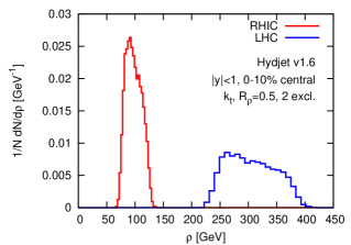
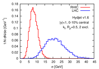
Figure 2: Distribution of the background density $\rho$ per unit area (left) and its intra-event fluctuations $\sigma$ (right). It has been obtained from 5000 HYDJET events with RHIC (AuAu, $\sqrt{s_{NN}}=200\,\mathrm{GeV}$) and LHC (PbPb, $\sqrt{s_{NN}}=5.5\,\mathrm{TeV}$) kinematics. The background properties have been estimated using the techniques presented in section 3.5, using the $k_{t}$ algorithm with $R_{\rho}=0.5$, and keeping only the jets with $|y|<1$ (excluding the two hardest).

As mentioned already in section 3.3, for the simulation of the events, we have used PYTHIA 6.4 [23] to generate the unquenched hard jets; the background events are generated using HYDJET v1.6 [19] with 0-10% centrality. Our setup for the background leads, for RHIC (AuAu, $\sqrt{s_{NN}}=200\,\mathrm{GeV}$), to an average background density per unit area at central rapidity of $\langle\rho\rangle\simeq 99$ GeV with average fluctuations in a single event of $\langle\sigma\rangle\simeq 8$ GeV and event-to-event fluctuations $\sigma_{\rho}\equiv\sqrt{\langle\rho^{2}\rangle-\langle\rho\rangle^{2}}\simeq 14$ GeV. For the LHC (PbPb, $\sqrt{s_{NN}}=5.5\,\mathrm{TeV}$) the corresponding values are $\langle\rho\rangle\simeq 310$ GeV, $\langle\sigma\rangle\simeq 20$ GeV and event-to-event fluctuations $\sigma_{\rho}\simeq 45$ GeV. Fig. 2 shows the distributions obtained from the simulations for $\rho$ and $\sigma$.

In the case of the RHIC simulation, the result for $\left\langle\rho\right\rangle$ is somewhat higher than the experimental value of $75\,\mathrm{GeV}$ quoted by the STAR collaboration [18], however this is probably in part due to limited tracking efficiencies at low $p_{t}$ at STAR, and explicit STAR [30] and PHENIX [31] results for $dE_{t}/d\eta$ correspond to somewhat higher $\rho$ values, about $90\,\mathrm{GeV}$. The multiplicity of charged particles ($dN_{ch}/d\eta\simeq 660$ for $\eta=0$ and 0–6% centrality) and the pion $p_{t}$ spectrum in our simulation are sensible compared to experimental measurements at RHIC [32, 33, 34]. For the LHC our charged particle multiplicity is $dN_{ch}/d\eta\simeq 1600$ for $\eta=0$ and 0–10% centrality, which is comparable to many of the predictions reviewed in fig. 7 of [35].

An independent control analysis has also been performed with HYDJET++ 2.1 [20] (with default parameters) for the background. The results at RHIC are similar, while for LHC the comparison is difficult because the default tune of HYDJET++ 2.1 predicts a much higher multiplicity, $dN_{ch}/d\eta\simeq 2800$ for $\eta=0$ and 0–10% centrality.

Most of the results of this section will be obtained without quenching, though in section 4.5 we will also consider the impact on our conclusions of the PYQUEN [19] and QPYTHIA [24] simulations of quenching effects.

For the results presented below, we have employed a selection cut of $|y|\leq y_{\rm max}$ on the jets with $y_{\rm max}=1$ for RHIC and $y_{\rm max}=2.4$ for the LHC. We only consider full jets that are matched to one of the two hardest jets in the hard event. The computation of the jet areas in FastJet, needed both for the subtraction and the background estimation, has been performed using active areas, with ghosts up to $y_{\rm max}+1.8$, a single repetition and a ghost area of 0.01. The determination of the background density $\rho$ has been performed using the $k_{t}$ algorithm with $R_{\rho}=0.5$. Though the estimate of the background depends on $R_{\rho}$ [16], we have observed that choices between 0.3 and 0.5 lead to very similar results (e.g. differing by at most a few hundred MeV at RHIC).

With this setup, we have studied the various ranges presented in section 3.5, with the jet algorithms from section 3.4. In all cases, we have taken the radius parameter $R=0.4$. We have adopted this value as it is the largest currently used at RHIC. Note that the effect of the background fluctuations of the jet energy resolution increases linearly with $R$, disfavouring significantly larger choices. On the other hand, too small a choice of $R$ may lead to excessive sensitivity to the details of parton fragmentation, hadronisation and detector granularity.

4.1 Matching efficiency

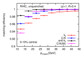
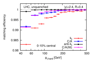
Figure 3: Matching efficiency for reconstructed jets as a function of the jet $p_{t}$. Left: RHIC, right: LHC. These results are independent of the choice of background-subtraction range in the heavy-ion events, since background subtraction does not enter into the matching criterion. Here and in later figures, the label “unquenched” refers to the embedded $pp$ event; the background is always simulated including quenching.

Let us start the presentation of our results with a brief discussion of the efficiency of reconstructing jets in the medium. As explained in section 3.2, the jets in the medium are matched to a “bare” hard jet when their common particle content accounts for at least 50% of the latter’s transverse momentum.

The matching efficiencies we observe depend to some extent on the details of the Monte Carlo used for the background so our intention is just to illustrate the typical behaviour we observe and highlight that these efficiencies tend to be large. We observe from fig. 3 that we successfully match at least 95% of the jets above $p_{t}\simeq 15$ GeV at RHIC, and at least 99% of the jets above $p_{t}\simeq 60$ GeV at the LHC. It is also interesting to notice that the anti-$k_{t}$ algorithm performs best, likely as a consequence of its ‘rigidity’, namely the fact that anti-$k_{t}$ jets tend to have the same (circular) shape, independently of the soft-particles that are present.

4.2 Choice of background-estimation range

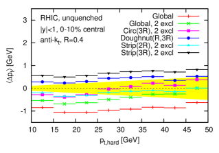
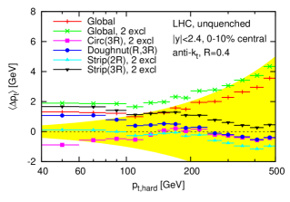
Figure 4: Effect of the choice of range on the average $p_{t}$ shift, $\Delta p_{t}$, as defined in eq. (1). Left: RHIC, right: LHC. In this figure and those that follow, the yellow band corresponds to 1% of the $p_{t}$ of the hard jet.

We now turn to the results concerning the measurement of the background density and the reconstruction of the jet transverse momentum. We first concentrate on the impact of the choice of a local range and/or of the exclusion of the two hardest jets when determining $\rho$.

In fig. 4 we show the average shift $\left\langle\Delta p_{t}\right\rangle$ for the list of ranges mentioned in section 3.5. The results presented here have been obtained with the anti-$k_{t}$ algorithm with $R=0.4$, but the differences among the various range choices have been seen to be similar with other jet definitions. The label “2 excl” means that the two hardest jets in the event have been excluded from the estimation of the background. We have found that this improves the precision of the subtractions whenever expected, i.e. for all choices of range except the doughnut range, where its central hole already acts similarly to the exclusion of the hardest jets. To keep the figure reasonably readable, we have only explicitly shown the effect of removing the two hardest jets for the global range. The change of 0.4–0.6 GeV (both for RHIC and the LHC) is in reasonable agreement with the analytic estimate of about 0.6 GeV for RHIC and the LHC obtained from $\left\langle\Delta p_{t}\right\rangle=\pi R^{2}\left\langle\Delta\rho\right\rangle$ with $\left\langle\Delta\rho\right\rangle$ calculated using eq. (7). Note that at LHC the exclusion of the two hardest jets for the global range appears to worsen the subtraction, however what is really happening is that the removal of the two hardest jets exacerbates a deficiency of the global range, namely the fact that its broad rapidity coverage causes it to underestimate $\rho$, leading to a positive net $\left\langle\Delta\rho\right\rangle$.

Other features that can be understood qualitatively include for example the differences between the two strip and the global (2 excl) range for RHIC: while the rapidity width of the global range lies in between that of the two strip ranges, the global range gives a lower $\left\langle\Delta p_{t}\right\rangle$ than both, corresponding to a larger $\rho$ estimate, which is reasonable because the global range is centred on $y=0$, whereas the strip ranges are mostly centred at larger rapidities where the background is lower.

The main result of the analysis of fig. 4 is the observation that all choices of a local range lead to a small residual $\Delta p_{t}$ offset: the background subtraction typically leaves a $|\left\langle\Delta p_{t}\right\rangle|\lesssim 1\,\mathrm{GeV}$ at both RHIC and LHC, i.e. better than 1-2% accuracy over much of the $p_{t}$ range of interest. It is not clear, within this level of accuracy, if one range is to be preferred to another, nor is it always easy to identify the precise origins of the observed differences between various ranges. Another way of viewing this is that the observed differences between the various choices give an estimate of the residual subtraction error due to possible misestimation of $\rho$. For our particular analysis, at RHIC this comment also applies to the choice of the global range (with the exclusion of the two hardest jets in the event). This is a consequence of the limited rapidity acceptance, which effectively turns the global range into a local one, a situation that does not hold for larger rapidity acceptances, as we have seen for the LHC results. In what follows we will use the Doughnut($R,3R$) choice, since it provides a good compromise between simplicity and effectiveness.

4.3 Choice of algorithm

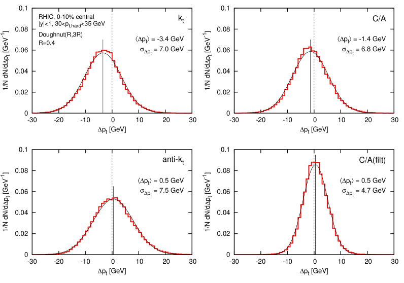
Figure 5: Distribution of $\Delta p_{t}$ (red histograms) for each of our 4 jet algorithms, together with a Gaussian (black curve) whose mean (solid vertical line) and dispersion are equal to $\left\langle\Delta p_{t}\right\rangle$ and $\sigma_{\Delta p_{t}}$ respectively.

The next potential systematic effect that we consider is the choice of the jet algorithm used for the clustering. Fig. 5 shows the distribution of $\Delta p_{t}$ for each of our four choices of jet algorithm, $k_{t}$, C/A, anti-$k_{t}$ and C/A(filt), given for RHIC collisions and a specific bin of the hard jets’ transverse momenta, $30<p_{t,\mathrm{hard}}<35\,\mathrm{GeV}$. One sees significant differences between the different algorithms. One also observes that Gaussians with mean and dispersion set equal to $\left\langle\Delta p_{t}\right\rangle$ and $\sigma_{\Delta p_{t}}$ provide a fair description of the full histograms. This validates our decision to concentrate on $\left\langle\Delta p_{t}\right\rangle$ and $\sigma_{\Delta p_{t}}$ as quality measures. One should nevertheless be aware that in the region of high $|\Delta p_{t}|$ there are deviations from perfect Gaussianity, which are more visible if one replicates fig. 5 with a logarithmic vertical scale (not shown, for brevity).

4.3.1 Average $\Delta p_{t}$

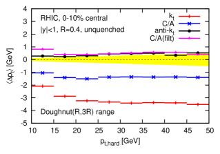
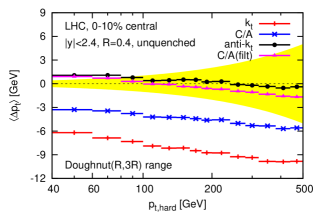
Figure 6: Average shift $\left\langle\Delta p_{t}\right\rangle$, as a function of $p_{t,\mathrm{hard}}$, shown for RHIC (left) and the LHC (right).

The first observable we analyse is the average $p_{t}$ shift. We show in fig. 6 the $\langle\Delta p_{t}\rangle$ results for the four algorithms listed in section 3.4, as a function of $p_{t,\mathrm{hard}}$. We use the doughnut range to estimate the background. The first observation is that, while the anti-$k_{t}$ and C/A(filt) algorithms have a small residual $\left\langle\Delta p_{t}\right\rangle$, the C/A and $k_{t}$ algorithms display significant offsets. The reason for the large offsets of $k_{t}$ and C/A is well understood, related to an effect known as back-reaction [15]. This is the fact that the addition of a soft background can alter the clustering of the particles of the hard event: some of the constituents of a jet in the hard event can be gained by or lost from the jet when clustering the event with the additional background of the full event. This happens, of course, on top of the simple background contamination that adds background particles to the hard jet. Even if this latter contamination is subtracted exactly, the reconstructed $p_{t}$ will still differ from that of the original hard jet as a consequence of the back-reaction.

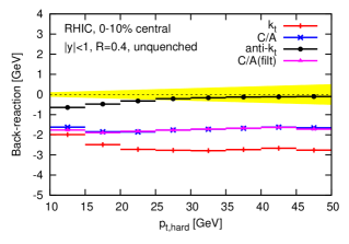
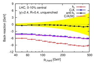
Figure 7: Contribution to $\left\langle\Delta p_{t}\right\rangle$ due to back-reaction. Note that these results are independent of the range used for estimating $\rho$ in the heavy-ion event. Left: RHIC, right: LHC.

The effect of the back-reaction can be studied in detail, since in Monte Carlo simulations it is possible to identify which hard-event constituents are present in a given jet before and after inclusion of the background particles in the clustering. The average $p_{t}$ shift due to back-reaction can be seen in fig. 7 for the different jet algorithms. As expected [15, 3], it is largest for $k_{t}$, and smallest (almost zero, in fact) for anti-$k_{t}$. By comparing fig. 7 and fig. 6 one can readily explain the difference between the $\left\langle\Delta p_{t}\right\rangle$ offsets of the various algorithms in terms of their back-reaction. The rigidity (and hence small back-reaction) of the anti-$k_{t}$ jets manifestly gives almost bias-free reconstructed jets, while the large back-reaction effects of the $k_{t}$ algorithm and, to a smaller extent, of the C/A algorithm translates into a worse performance in terms of average shift. The $p_{t}$ dependence of the back-reaction is weak. This is expected based on the interplay between the $\ln\ln p_{t}$ dependence found in [15] and the evolution with $p_{t}$ of the relative fractions of quark and gluon jets.

The case of the C/A(filt) algorithm is more complex: its small net offset, comparable to that of the anti-$k_{t}$ algorithm, appears to be due to a fortuitous compensation between an under-subtraction of the background and a negative back-reaction. The negative back-reaction is very similar to that of C/A without filtering, while the under-subtraction is related to the fact that the selection of the hardest subjets introduces a bias towards positive fluctuations of the background. This effect is discussed in Appendix B, where we obtain the following estimate for the average $p_{t}$ shift (specifically for $R_{\rm filt}=R/2$):

$$\left\langle(\Delta p_{t})_{\rm filt}\right\rangle\simeq 0.56\,R\sigma,$$ (8)

yielding an average bias of 2 GeV for RHIC and 4.5 GeV at the LHC, which are both in good agreement with the differences observed between C/A with and without filtering in fig. 6. Note that while the bias in eq. (8) is proportional to $\sigma$, the back-reaction bias is instead mainly proportional to $\rho$ [15]. It is because of these different proportionalities that the cancellation between the two effects should be considered as fortuitous. Since it also depends on the substructure of the jet, one may also expect that the cancellation that we see here could break down in the presence of quenching.

4.3.2 Dispersion of $\Delta p_{t}$

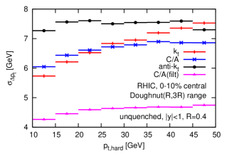
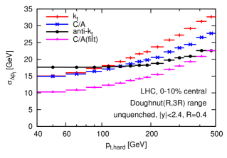
Figure 8: Dispersion $\sigma_{\Delta p_{t}}$. Left: RHIC, right: LHC.

Our results for the $\Delta p_{t}$ dispersion, $\sigma_{\Delta p_{t}}$, are shown in fig. 8, again using the doughnut range. (Our conclusions are essentially independent of the particular choice of range.)

We first discuss the case of RHIC kinematics. For $k_{t}$ and anti-$k_{t}$, the observed dispersions are similar to the result of $6.8\,\mathrm{GeV}$ quoted by STAR [18] (though the number from STAR includes detector resolution effects, so that the true physical $\sigma_{\Delta p_{t}}$ may actually be somewhat lower). Of note, the advantage enjoyed by anti-$k_{t}$ in terms of smallest $\left\langle\Delta p_{t}\right\rangle$ does not hold at the level of the dispersion: C/A and $k_{t}$ tend to behave slightly better at small transverse momentum. The algorithm which performs best in terms of dispersion over all the $p_{t}$ range is now C/A with filtering, for which the result is smaller than that of the other algorithms by a factor of about $1/\sqrt{2}$. This reduction factor can be explained because the dispersion $\sigma_{\Delta p_{t}}$ is expected to be proportional to the square-root of the jet area: the C/A(filt) algorithm with $R_{\rm filt}=R/2$ and $n_{\rm filt}=2$ produces jets with an area of, roughly, half that obtained with C/A; hence the observed reduction of $\sigma_{\Delta p_{t}}$.

In the LHC setup, the conclusions are quite similar at the lowest transverse momenta shown. As $p_{t}$ increases, the dispersion of the anti-$k_{t}$ algorithm grows slowly, while that of the others grows more rapidly, so that at the highest $p_{t}$’s shown, the $k_{t}$ and C/A algorithms have noticeably larger dispersions than anti-$k_{t}$, and C/A(filt) becomes similar to anti-$k_{t}$. The growth of the dispersions can be attributed to an increase of the back-reaction dispersion. The latter is dominated by rare occurrences, where a large fraction of the jet’s $p_{t}$ is gained or lost to back-reaction, hence the noticeable $p_{t}$ dependence (cf. appendix C.1). An additional effect, especially for the $k_{t}$ algorithm, might come from the anomalous dimension of the jet areas, i.e. the growth with $p_{t}$ of the average jet area.

Note that the dispersion has some limited dependence on the choice of ghost area — for example, reducing it from 0.01 to 0.0025 lowers the dispersions by about $0.2-0.4\,\mathrm{GeV}$ at RHIC. This is discussed further in appendix C.2.

4.4 Centrality dependence

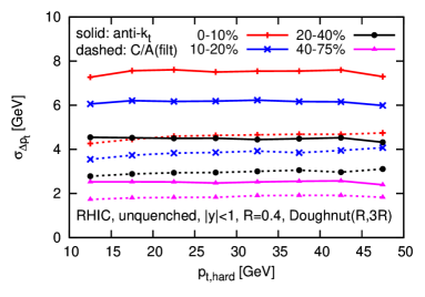
Figure 9: $p_{t}$ dependence dependence of the $\Delta p_{t}$ dispersion at RHIC, for different centrality classes.

So far, we have only considered central collisions. Since it is known that non-central collisions give rise to elliptic flow [36, 37], one might worry that this leads to an extra source of background fluctuations and/or non-uniformities, potentially spoiling the subtraction picture discussed so far. One can study this on azimuthally averaged jet samples (as we have been doing so far) or as a function of the azimuthal angle, $\Delta\phi$, between the jet and the reaction plane. As above, we use HYDJET v1.6, whose underlying HYDRO component includes a simulation of elliptic flow [38].

We have generated heavy-ion background events for RHIC in four different centrality bins: 0-10% (as above), 10-20%, 20-40% and 40-75%, with $v_{2}$ values respectively of $1.7\%$, $3.3\%$, $5.0\%$ and $5.3\%$.

We first examine azimuthally averaged results, repeating the studies of the previous sections for each of the centrality bins. We find that the results for the average shift, $\left\langle\Delta p_{t}\right\rangle$, are largely independent of centrality, as expected if the elliptic flow effects disappear when averaged over $\phi$. The results for the dispersion are shown in fig. 9. We observe that the dispersion decreases with increasing non-centrality. Even though one might expect adverse effects from elliptic flow, the heavy-ion background decreases rapidly when one moves from central to peripheral collisions, and this directly translates into a decrease of $\sigma_{\Delta p_{t}}$.

The first conclusion from this centrality-dependence study is therefore that the subtraction methods presented in this paper appear to be applicable also for azimuthally averaged observables in non-central collisions.

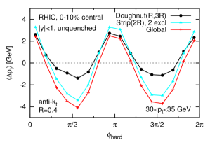
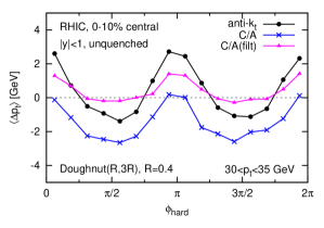
Figure 10: $\phi$ dependence of the $\Delta p_{t}$ shift at RHIC, for the $0-10\%$ centrality bin. Left: for three different ranges for the anti-$k_{t}$ algorithm; right: for three different jet algorithms for the doughnut($R,3R$) range. The absolute size of the $\phi$ dependence is similar for centralities up to $40\%$ and then decreases beyond.

We next consider results as a function of $\Delta\phi$, which is relevant if one wishes to examine the correlation between jet quenching and the reaction plane. An issue in real experimental studies is the determination of the reaction plane, and the extent to which it is affected by the presence of hard jets. In the HYDJET simulations, this problem does not arise because the reaction plane always corresponds to $\phi=0$. Figure 10 (left) shows the average $\Delta p_{t}$ as a function of $\Delta\phi$ for the anti-$k_{t}$ algorithm and several different background-estimation ranges, for the $0-10\%$ centrality bin for RHIC. The strip range shows significant $\Delta\phi$ dependence, which is because a determination of $\rho$ averaged over all $\phi$ cannot possibly account for the local $\phi$-dependence induced by the elliptic flow. Other ranges, such as the doughnut range, instead cover a more limited region in $\phi$. They should therefore be able to provide information on the $\phi$-dependence of the background. However, since their extent in $\phi$ tends to be significantly larger than that of the jet, and $\rho$ varies relevantly over that extent, some residual $\phi$ dependence remains in $\left\langle\Delta p_{t}\right\rangle$ after subtraction. The right-hand plot of figure 10 shows that the effect is reduced with filtering, as is to be expected since its initial background contamination is smaller. The conclusion from this part of the study is that residual $\phi$-dependent offsets may need to be corrected for explicitly in any studies of jets and their correlations with the reaction plane. The investigation of extensions to our background subtraction procedure to address this issue will be the subject of future work.

4.5 Quenching effects

The last issue we wish to investigate is how the phenomenon of jet quenching (i.e. medium effects on parton fragmentation) may affect the picture developed so far. The precise nature of jet quenching beyond its basic analytic properties (see e.g. [21]) is certainly hard to estimate in detail, especially at the LHC, where experimental data from, say, flow or particle spectra measurements are not yet available for the tuning of the Monte Carlo simulations. Additionally, the implementation of Monte-Carlo generators that incorporate the analytic features of jet quenching models is currently a very active field [24, 39, 40]. We may therefore expect a more robust and complete picture of jet quenching in the near future, together with the awaited first PbPb collisions at the LHC.

In this section, we examine the robustness of our HI background subtraction in the presence of (simulated) jet quenching. For this purpose we have used two available models which allow one to simulate quenched hard jets, PYQUEN [19], which is used by HYDJET v1.6, and QPYTHIA [24]. PYQUEN has been run with the parameters listed in footnote 7 for the LHC, and with $\texttt{T0}=0.5\,\mathrm{GeV}$, $\texttt{tau0}=0.4$ fm and $\texttt{nf}=2$ for RHIC. For QPYTHIA we have tested two options for the values of the transport coefficient and the medium length ($\hat{q}=3$ GeV²/fm, $L=5$ fm and $\hat{q}=1$ GeV²/fm, $L=6$ fm), with similar results. No serious attempt has been made to tune the two codes with each other or with the experimental data, beyond what is already suggested by the code defaults: in the absence of strong experimental constraints on the details of the quenching effects, this allows us to verify the robustness of our results for a range of conditions.

As in sections 4.2 and 4.3, we have embedded the hard PYQUEN or QPYTHIA events in a HYDJET v1.6 background and tested the effectiveness of the background subtraction for different choices of algorithm. We shall restrict our attention to the anti-$k_{t}$ and C/A(filt) algorithms, as they appear to be the optimal choices from our analysis so far.

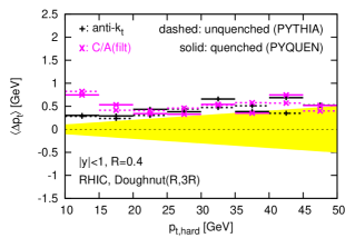
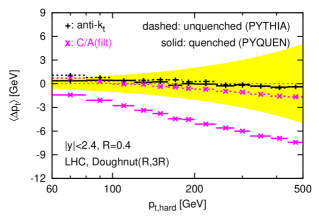
Figure 11: Average $p_{t}$ shift for background-subtracted jets with the anti-$k_{t}$ and C/A(filt) jet algorithms. The dashed lines correspond to unquenched hard jets (PYTHIA) and the solid ones to quenched hard jets (PYQUEN). Results are shown for RHIC kinematics on the left plot and for the LHC on the right one.

We have found that the jet-matching efficiencies are still high, with essentially no changes at RHIC, and at LHC a doubling of the (small) inefficiencies that we saw in fig. 3(right). The dispersions $\sigma_{\Delta p_{t}}$ are also not significantly affected within our sample of jet-quenching simulations. We therefore concentrate on the $\left\langle\Delta p_{t}\right\rangle$ offset, which is plotted in fig. 11 for PYQUEN. The results are shown for both RHIC and the LHC. In the case of RHIC, and for the whole $p_{t}$ range up to about 50 GeV, quenching can be seen not to significantly affect the subtraction offset $\langle\Delta p_{t}\rangle$ (within the usual uncertainty related to the choice of range, which was shown in fig. 4). In the LHC case, instead, while the shift obtained using the anti-$k_{t}$ algorithm is largely similar to the unquenched case, the C/A(filt) algorithm performance can be seen to deteriorate slightly when quenching is turned on, all the more so at very large transverse momentum. The $k_{t}$ and the C/A algorithms are not shown for clarity, but they share the behaviour of C/A(filt). This deterioration of the quality of the subtraction can be traced back to an increased back-reaction compared to the unquenched jets. Anti-$k_{t}$ jets do not suffer from this effect as a consequence of the usual rigidity of this algorithm. In the case of C/A(filt), one should nevertheless emphasise that an error of (at most) 10 GeV on the reconstruction of a 500 GeV jet is still only a 2% effect. This is modest, both relative to the likely experimental precision and to the expected effect of quenching on the overall jet $p_{t}$, predicted by PYQUEN to be at the level of $10\%$ at this $p_{t}$.

Though for brevity we have not explicitly shown them, the results with QPYTHIA are very similar.

Before closing this section, we reiterate that we have only investigated simple models for quenching and that our results are meant just to give a first estimate of the effects that one might have to deal with in the case of quenched jets. The expected future availability of new “quenched” Monte Carlo programs, together with specific measurements in the early days of heavy-ion collisions at the LHC, will certainly allow one to address this question more extensively.

4.6 Relative importance of average shift and dispersion

To close this section, we examine the relative importance of the average shift and its dispersion, taking the illustrative example of their impact on the inclusive jet cross-section as a function of $p_{t}$. We start from a simple parametrisation of the inclusive-jet $p_{t}$ spectrum and see how its reconstruction is affected by the average shift and dispersion that remain for $\Delta p_{t}$ after subtraction.

Let us assume that the true $p_{t}$ spectrum decays exponentially i.e.

$$\frac{d\sigma^{pp}}{dp_{t}}=\sigma_{0}\lambda\,e^{-\lambda p_{t}}.$$ (9)

While this expression doesn’t have the $1/p_{t}^{n}$ form that one expects to see, it is far easier to handle analytically, and not too poor an approximation to observed spectra over quite a broad range of $p_{t}$. After embedding the hard events in a heavy-ion background and applying subtraction, the resulting spectrum will be the convolution of eq. (9) with the $\Delta p_{t}$ distribution. Assuming that the latter is a Gaussian of average $\left\langle\Delta p_{t}\right\rangle$ and dispersion $\sigma_{\Delta p_{t}}$ (cf. fig. 5), one obtains a reconstructed spectrum

$$\frac{d\sigma^{AA,\rm sub}}{dp_{t}}=\exp\left(\lambda\left\langle\Delta p_{t}\right\rangle+\frac{\lambda^{2}\sigma_{\Delta p_{t}}^{2}}{2}\right)\,\frac{d\sigma^{pp}}{dp_{t}}.$$ (10)

Thus the average shift gives a bias by a multiplicative factor $\exp(\lambda\left\langle\Delta p_{t}\right\rangle)$ and the dispersion by a factor $\exp(\lambda^{2}\sigma_{\Delta p_{t}}^{2}/2)$. The convolution works in such a way that for a given reconstructed $p_{t}$, the most likely original true transverse momentum is:

$$\text{most likely}\;p_{t}^{pp}\simeq p_{t}^{AA,{\rm sub}}-\left\langle\Delta p_{t}\right\rangle-\lambda\sigma_{\Delta p_{t}}^{2}\,,$$ (11)

where we have neglected the small impact of subtraction on the $pp$ jets.

To illustrate these effects quantitatively, let us first take the example of RHIC, where between 10 and 60 GeV, the cross-section is well approximated by eq. (9) with $\lambda=0.3$ GeV^-1. Both the anti-$k_{t}$ and C/A(filt) have $\left\langle\Delta p_{t}\right\rangle\simeq 0$, leaving only the dispersion effect. In the case of the anti-$k_{t}$ (respectively C/A(filt)) algorithm, we see from fig. 8 that $\sigma_{\Delta p_{t}}\simeq 7.5\,\mathrm{GeV}$ ($4.8\,\mathrm{GeV}$), which gives a multiplicative factor of about 12 (3). For a given reconstructed $p_{t}$, the most likely true $p_{t}$ is about $17\,\mathrm{GeV}$ ($7\,\mathrm{GeV}$) smaller. In comparison, for C/A ($k_{t}$), with $\left\langle\Delta p_{t}\right\rangle\simeq-1.5\,\mathrm{GeV}$ ($-3.5\,\mathrm{GeV}$) (fig. 6) and $\sigma_{\Delta p_{t}}\simeq 6.5\,\mathrm{GeV}$ (similar for $k_{t}$) there is a partial compensation between factors of $0.64$ ($0.35$) and $6.7$ coming respectively from the shift and dispersion, yielding an overall factor of about $4$ ($2.3$), while the most likely true $p_{t}$ is about $14\,\mathrm{GeV}$ ($12\,\mathrm{GeV}$) smaller than the reconstructed $p_{t}$.

At the LHC ($\sqrt{s_{NN}}=5.5\,\mathrm{TeV}$), eq. (9) is a less accurate approximation. Nevertheless, for $p_{t}\sim 100-150\,\mathrm{GeV}$, it is not too unreasonable to take $\lambda=0.05\,\mathrm{GeV}^{-1}$ and examine the consequences. For anti-$k_{t}$ (respectively C/A(filt)), we have $\left\langle\Delta p_{t}\right\rangle\simeq 0$ (also for C/A(filt)) and $\sigma_{\Delta p_{t}}\simeq 18\,\mathrm{GeV}$ ($13\,\mathrm{GeV}$), giving a multiplicative factor of $1.5$ ($1.2$), i.e. far smaller corrections than at RHIC. For a given reconstructed $p_{t}$, the most likely true $p_{t}$ is about $16\,\mathrm{GeV}$ ($8\,\mathrm{GeV}$) smaller, rather similar to the values we found at RHIC (though smaller in relative terms, since the $p_{t}$’s are higher), with the increase in $\sigma$ being compensated by the decrease in $\lambda$.

In the LHC case, it is also worth commenting on the results for the $k_{t}$ algorithm, since this is what was used in ref. [14]: we have $\left\langle\Delta p_{t}\right\rangle\simeq-8\,\mathrm{GeV}$ and $\sigma_{\Delta p_{t}}\simeq 18\,\mathrm{GeV}$, giving a multiplicative factor of $1.05$, which is consistent with the near perfect agreement that was seen there between the $pp$ and subtracted $AA$ spectra. That agreement does not however imply perfect reconstruction, since the most likely $p_{t}^{pp}$ is about $7\,\mathrm{GeV}$ lower than $p_{t}^{AA,{\rm sub}}$.

Though the above numbers give an idea of the relative difficulties of using different algorithms at RHIC and LHC, experimentally what matters most will be the systematic errors on the correction factors (for example due to poorly understood non-Gaussian tails of the $\Delta p_{t}$ distribution). Note also that a compensation between shift and dispersion factors, as happens for example with the C/A algorithm, is unlikely to reduce the overall systematic errors.

5 The issue of fakes

While the goal of this paper is not to discuss the issue of “fake-jets” in detail, it is a question that has been the subject of substantial debate recently (see for example [9, 41]). Here, therefore, we wish to devote a few words to it and discuss how it relates to our background-subtraction results so far.

In a picture in which the soft background and the hard jets are independent of each other, one way of thinking about a fake jet is that it is a reconstructed jet (with significant $p_{t}$) that is due not to the presence of an actual hard jet, but rather due to an upwards fluctuation of the soft background. The difficulty with this definition is that there is no uniquely-defined separation between “hard” jets and soft background. This can be illustrated with the example of how HYDJET simulates RHIC collisions: one event typically consists of a soft HYDRO background supplemented with $\sim 60$ $pp$ collisions, each simulated with a minimum $p_{t}$ cut of $2.6\,\mathrm{GeV}$ on the $2\to 2$ scattering. To some approximation, the properties of the full heavy-ion events remain relatively unchanged if one modifies the number of $pp$ collisions and corresponding $p_{t}$ cut and also retunes the soft background. The fact that this changes the number of hard jets provides one illustration of the issue that the soft/hard separation is ill-defined. Additionally, while there are $\sim 60$ semi-hard $pp$ collisions ($\sim 120$ mostly central semi-hard jets) in an event, there is only space within (say) the acceptance of RHIC for ${\cal{O}}\left(40\right)$ jets. Thus there is essentially no region in an event which does not have a semi-hard jet. From this point of view, every reconstructed jet corresponds to a (semi-)hard $pp$ jet and there are no fake jets at all.

5.1 Inclusive analyses

For inclusive analyses, such as a measurement of the inclusive jet spectrum, this last point is particularly relevant, because every jet in the event contributes to the measurement. Then, the issue of fakes can be viewed as one of unfolding. In that respect it becomes instructive, for a given bin of the reconstructed heavy-ion $p_{t}$, to ask what the corresponding matched $pp$ jet transverse momenta were. Specifically, we define a quantity $O(p_{t}^{AA,{\rm sub}},p_{t}^{pp})$, the distribution of the $pp$ “origin”, $p_{t}^{pp}$, of a heavy-ion jet with subtracted transverse momentum $p_{t}^{AA,{\rm sub}}$. If the origin $O(p_{t}^{AA,{\rm sub}},p_{t}^{pp})$ is dominated by a region of $p_{t}^{pp}$ of the same order as $p_{t}^{AA,{\rm sub}}$, then that tells us that the jets being reconstructed are truly hard. If, on the other hand, it is dominated by $p_{t}^{pp}$ near zero, then that is a sign that apparently hard heavy-ion jets are mostly due to upwards fluctuations of the background superimposed on low-$p_{t}$ $pp$ jets, making the unfolding more delicate.

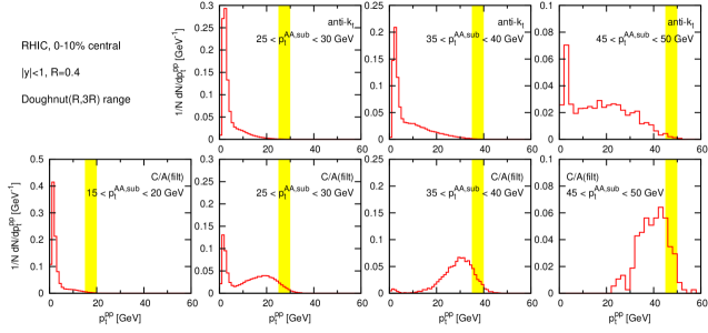
Figure 12: The $p_{t}$ distribution of the $pp$ jet corresponding to a given bin of reconstructed heavy-ion jet $p_{t}^{AA,{\rm sub}}$ at RHIC, i.e. $O(p_{t}^{AA,{\rm sub}},p_{t}^{pp})$ as a function of $p_{t}^{pp}$ for a given bin of $p_{t}^{AA,{\rm sub}}$. The upper row is for the anti-$k_{t}$ algorithm, while the lower row is for C/A(filt). Each column corresponds to a different $p_{t}^{AA,{\rm sub}}$ bin, as indicated by the vertical band in each plot. Cases in which the histogram is broad or peaked near $0$ are indicative of the need for special care in the unfolding procedure. These plots were generated using approximately 90 million events. Each plot has been normalised to the number of events in the corresponding $p_{t}^{AA,{\rm sub}}$ bin.

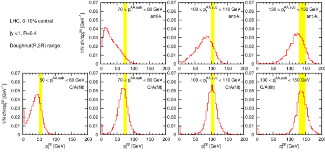
Figure 13: Same as fig. 12 for LHC kinematics (PbPb, $\sqrt{s}=5.5\,\mathrm{TeV}$), generated with approximately 16 million events. Note the use of a smaller rapidity range here, $|y|<1$, compared to the earlier LHC plots.

In figure 12 we show the origins of heavy-ion jets as determined in our HYDJET simulations. The upper row provides the origin plots for anti-$k_{t}$ jets at RHIC. Each plot corresponds to one bin of $p_{t}^{AA,{\rm sub}}$, and shows $O(p_{t}^{AA,{\rm sub}},p_{t}^{pp})$ as a function of $p_{t}^{pp}$. At moderate $p_{t}^{AA,{\rm sub}}$, the $25-30\,\mathrm{GeV}$ bin, the origin is dominated by low $p_{t}^{pp}$. This is perhaps not surprising, given the result in section 4.6 that the $p_{t}^{pp}$ origin is expected to be $\sim 17\,\mathrm{GeV}$ lower than $p_{t}^{AA,{\rm sub}}$ for anti-$k_{t}$ jets — additionally, that result assumed an exponential spectrum for the inclusive jet distribution, whereas the distribution rises substantially faster towards low $p_{t}^{pp}$. As $p_{t}^{AA,{\rm sub}}$ increases one sees that the contribution of high $p_{t}^{pp}$ jets increases, in a manner not too inconsistent with the expected $\sim 17\,\mathrm{GeV}$ shift, though the $p_{t}^{pp}$ distribution remains rather broad and a peak persists at small $p_{t}^{pp}$. These plots suggest that an inclusive jet distribution measurement with the anti-$k_{t}$ algorithm at RHIC is not completely trivial since, up to rather large $p_{t}^{AA,{\rm sub}}$, one is still sensitive to the jet distribution at small values of $p_{t}^{pp}$ where the separation between “hard” jets and the soft medium is less clear. Nevertheless, two points should be kept in mind: firstly, the upper row of fig. 12 shows that different $p_{t}^{AA,{\rm sub}}$ have complementary sensitivities to different parts of the $p_{t}^{pp}$ spectrum. Thus it should still be possible to “unfold” the $p_{t}^{AA,{\rm sub}}$ distribution to obtain information about the $p_{t}^{pp}$, unfolding being in any case a standard part of the experimental correction procedure. Secondly STAR quotes [18] a $10\%$ smaller value for $\sigma_{\Delta p_{t}}$ than the $7.5\,\mathrm{GeV}$ that we find in HYDJET. Such a reduction can make it noticeably easier to perform the unfolding.

The impact of a reduction in $\sigma_{\Delta p_{t}}$ is illustrated in the lower row of fig. 12, which shows the result for C/A(filt). Here, even the $25-30\,\mathrm{GeV}$ bin for $p_{t}^{AA,{\rm sub}}$ shows a moderate-$p_{t}$ peak in the distribution of $p_{t}^{pp}$, and in the $35-40\,\mathrm{GeV}$ bin the low-$p_{t}$ “fake” peak has disappeared almost entirely. Furthermore, the $p_{t}^{pp}$ peak is centred about $7\,\mathrm{GeV}$ lower than the centre of the $p_{t}^{AA,{\rm sub}}$ bin, remarkably consistent with the calculations of section 4.6. Overall, therefore, unfolding with C/A(filt) will be easier than with anti-$k_{t}$.

Corresponding plots for the LHC are shown in fig. 13. While C/A(filt)’s lower dispersion still gives it an advantage over anti-$k_{t}$, for $\smash{p_{t}^{AA,{\rm sub}}}\gtrsim 80\,\mathrm{GeV}$, anti-$k_{t}$ does now reach a domain where the original $pp$ jets are themselves always hard.

Procedures to reject fake jets have been proposed, in [10, 11]. They are based on a cut on (collinear unsafe) jet shape properties and it is thus unclear how they will be affected by quenching and in particular whether the expected benefit of cutting the low-$p_{t}^{pp}$ peak in figs. 12 and 13 outweighs the disadvantage of potentially introducing extra sources of systematic uncertainty at moderate $p_{t}$.

One final comment is that experimental unfolding should provide enough information to produce origin plots like those shown here. As part of the broader discussion about fakes it would probably be instructive for such plots to be shown together with the inclusive-jet results.

5.2 Exclusive analyses

An example of an exclusive analysis might be a dijet study, in which one selects the two hardest jets in the event, with transverse momenta $p_{t1}$ and $p_{t2}$, and plots the distribution of $\frac{1}{2}H_{T,2}\equiv\frac{1}{2}(p_{t1}+p_{t2})$. Here one can define “fakes” as corresponding to cases where one or other of the jets fails to match to one of the two hardest among all the jets from the individual $pp$ events. This definition is insensitive to the soft/hard boundary in a simulation such as HYDJET, because it naturally picks out hard $pp$ jets that are far above that boundary. And, by concentrating on just two jets, it also evades the problem of high occupancy from the large multiplicity of semi-hard $pp$ collisions. This simplification of the definition of fakes is common to many exclusive analyses, because they tend to share the feature of identifying just one or two hard reference jets.

The specific case of the exclusive dijet analysis has the added advantage that it is amenable to a data-driven estimation of fakes. One divides the events into two groups, those for which the two hardest jets are on the same side (in azimuth) of the event and those in which they are on opposite sides (a related analysis was presented by STAR in ref. [42]). For events in which one of the two jets is “fake,” the two jets are just as likely to be on the same side as on the opposite side. This is not the case for non-fake jets, given that the two hardest “true” jets nearly always come from the same $pp$ event and so have to be on opposite sides. Thus by counting the number of same-side versus opposite-side dijets in a given $\frac{1}{2}H_{T,2}$ bin, one immediately has an estimate of the fake rate.

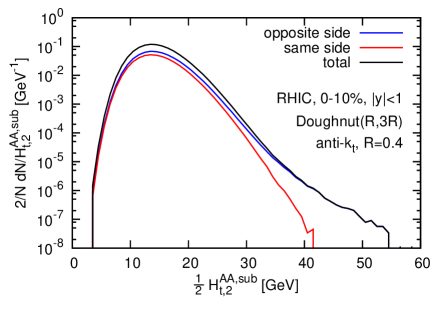
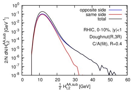
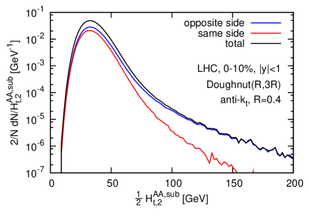
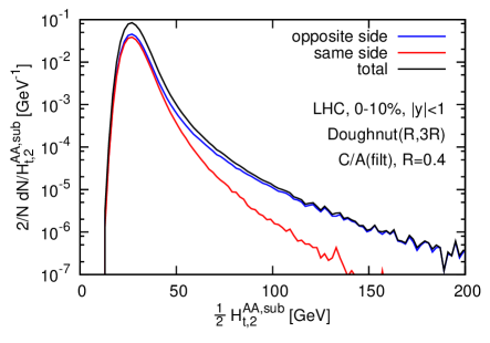
Figure 14: The distribution of $\frac{1}{2}H_{T,2}$ obtained from the two hardest full, subtracted heavy-ion jets in each event at RHIC, as obtained from simulations with HYDJET 1.6. The left-hand plot is for anti-$k_{t}$ and the right-hand plot for C/A(filt). The same-side curves give an approximate measure of (half of) the contribution of “fake” jets to the dijet spectrum.

Figure 15: Same as fig. 15 for LHC kinematics.

This is illustrated in fig. 15, which shows the distribution at RHIC of the full, subtracted $\frac{1}{2}H_{T,2}$ result, together with its separation into opposite-side and same-side components. One sees that in the peak region, the opposite and same-side distributions are very similar, indicating a predominantly “fake” origin for at least one of two hardest jets (they are not quite identical, because there is less phase-space on the same side for a second jet than there is on the away side). However above a certain full, reconstructed $\frac{1}{2}H_{T,2}$ value, about $30\,\mathrm{GeV}$ for anti-$k_{t}$ and $20\,\mathrm{GeV}$ for C/A(filt) the same-side distribution starts to fall far more rapidly than the opposite-side one, indicating that the measurement is now dominated by “true” pairs of jets.

The LHC results, fig. 15, are qualitatively similar, with the same-side spectrum starting to fall off more steeply than the opposite-side one around $70\,\mathrm{GeV}$ for the anti-$k_{t}$ algorithm and $50\,\mathrm{GeV}$ for C/A(filt).

One can also examine origin plots for $H_{T,2}$, in analogy with the Monte Carlo analysis of section 5.1. For brevity, we refrain from showing them here, and restrict ourselves to the comment that in the region of $H_{T,2}$ where the result is dominated by opposite-side pairs, the origin plots are consistent with a purely hard origin for the dijets.

6 Conclusions

In this article we have presented the results of a systematic study of heavy-ion jet reconstruction with jet-area based background subtraction, building on the brief initial proposal of [14].

The questions we have examined include those of the choice of range for estimating the background, the choice of algorithm for the jet finding and the robustness of the reconstruction with respect to quenching effects and collision centrality.

We have found that there is little difference between various ranges, as long as they are chosen to be localised to the vicinity of the jet of interest and of sufficient size (at least 4 units of area for jets with $R=0.4$). In comparing different algorithms we examined the systematic offset and the dispersion in the reconstructed jet $p_{t}$. The offset can be brought close to zero by using the anti-$k_{t}$ algorithm, while the $k_{t}$ algorithm has the largest offset; the Cambridge/Aachen (C/A) algorithm with filtering also gives a small offset, however this seems to have been due to a fortuitous cancellation between two only partially related effects. The dispersion is comparable for anti-$k_{t}$, C/A and $k_{t}$, but significantly smaller for C/A(filt) (except at high transverse momenta for LHC), as a consequence of its smaller jet area. Among the different algorithms, anti-$k_{t}$ is the most robust with respect to quenching effects, and C/A(filt) seems reasonably robust at RHIC, though a little less so at the LHC. The precise numerical results for offset and dispersion can depend a little on the details of the simulation and the analysis, however the general pattern remains.

Overall our results indicate that the area-based subtraction method seems well suited for jet reconstruction in heavy-ion collisions. Two jet-algorithm choices were found to perform particularly well: anti-$k_{t}$, which has small offsets but larger fluctuations, and C/A with filtering, for which the offsets may be harder to control, but for which the fluctuations are significantly reduced, with consequent advantages for the unfolding of experimentally measured jet spectra. Ultimately, we suspect that carrying out parallel analyses with these two choices may help maximise the reliability of jet results in HI collisions.

Appendix A Estimate of the minimal size of a range

A.1 Fluctuations in extracted $\rho$

In section 3.5, we gave an estimate of the minimum size of a range one should require for determining $\rho$, given a requirement that fluctuations in the determination of $\rho$ should be moderate. We give the details of the computation in this appendix.

We start from the fact that the error made on the estimation of the background density $\rho$ will translate into an increase of the dispersion $\sigma_{\Delta p_{t}}$: on one hand, the dominant contribution to $\sigma_{\Delta p_{t}}$ comes from the intra-event fluctuations of the background i.e. is of order $\sigma\sqrt{A_{\rm jet}}$ with $A_{\rm jet}$ the jet area; on the other hand, the dispersion $S_{\Delta\rho}$ of the misestimation of $\rho$ leads to an additional dispersion on the reconstructed jet $p_{t}$ of $S_{\Delta\rho}A_{\rm jet}$. Adding these two sources of dispersion in quadrature and using the result from section 3.4 of [16], $S_{\Delta\rho}\simeq\sqrt{\pi/(2A_{\cal R})}\sigma$ with $A_{\cal R}$ the area of the range under consideration, we get

$$\sigma_{\Delta p_{t}}\simeq\sigma\left(A_{\rm jet}+\frac{\pi A_{\rm jet}^{2}}{2A_{\cal R}}\right)^{\frac{1}{2}}.$$ (12)

If we ask e.g. that the contribution to the total dispersion coming from the misestimation of the background be no more than a fraction $\epsilon$ of the total $\sigma_{\Delta p_{t}}$, then we obtain the requirement

$$A_{\cal R}\gtrsim A_{\min}\simeq\frac{\pi}{4}\frac{A_{\rm jet}}{\epsilon}\,.$$ (13)

For anti-$k_{t}$ jets of radius $R$, with $A_{\rm jet}\simeq\pi R^{2}$, this translates to

$$A_{\cal R}\gtrsim\frac{\pi^{2}}{4}\frac{R^{2}}{\epsilon}\simeq 25R^{2}\,,$$ (14)

where the numerical result has been given for $\epsilon=0.1$. For $R=0.4$, it becomes $A_{\cal R}\gtrsim 4$.

We can also cast this result in terms of the number of jets that must be present in ${\cal R}$. Assuming that the jets used to estimate $\rho$ have a mean area of $0.55\pi R_{\rho}^{2}$, we find a minimal number of jets ,

$$n_{\min}\simeq\frac{A_{\min}}{0.55\pi R_{\rho}^{2}}\simeq\frac{1.4}{\epsilon}\frac{R^{2}}{R_{\rho}^{2}}\,,$$ (15)

where, as before, we have taken $A_{\mathrm{jet}}\simeq\pi R^{2}$. Taking the numbers quoted above and $R_{\rho}=0.5$, as used in the main body of the article, this gives $n_{\min}\simeq 9$.

A.2 Hard-jet bias in extracted $\rho$

From section 3.3 of [16], we know that the presence of hard jets and initial-state radiation leads to a bias in the extraction of $\rho$ of

$$\left\langle\Delta\rho\right\rangle\simeq\sigma R_{\rho}\sqrt{\frac{\pi c_{J}}{2}}\frac{\left\langle n_{h}\right\rangle}{A_{\cal R}}\,$$ (16)

where $c_{J}\simeq 2$ is a numerical constant and $\left\langle n_{h}\right\rangle$ is the average number of “hard” jets (those above the scale of the background fluctuations, including initial-state radiation); $\left\langle n_{h}\right\rangle$ is given by

$$\frac{\left\langle n_{h}\right\rangle}{A_{\cal R}}\simeq\frac{n_{b}}{A_{\cal R}}+\frac{C_{i}}{\pi^{2}}\frac{L}{b_{0}}\,,\qquad\quad L=\ln\frac{\alpha_{s}\left(\sqrt{c_{J}}\sigma R_{\rho}\right)}{\alpha_{s}(p_{t})}\,,$$ (17)

where $n_{b}$ is the number of “Born” partons from the underlying $2\to 2$ scattering that enter the region $\cal R$, while $b_{0}=(11C_{A}-2n_{f})/(12\pi)$ is the first coefficient of the QCD $\beta$-function. In the context of [16], principally directed towards a study of the UE in $pp$ collisions, $\sigma$ was rather small, causing the second term of eq. (17), associated with initial-state radiation above a scale $\sim\sigma R_{\rho}$, to be comparable in size to the first term. In our case, $\sigma$ is significantly larger and this reduces the impact of the second term sufficiently that we can ignore it. We thus arrive at the result

$$\left\langle\Delta\rho\right\rangle\simeq\sigma R_{\rho}\sqrt{\frac{\pi c_{J}}{2}}\frac{n_{b}}{A_{\cal R}}\simeq 1.8\,\sigma R_{\rho}\frac{n_{b}}{A_{\cal R}}\,.$$ (18)

Note that the presence of hard jets and initial-state radiation also affects the fluctuations in the misestimation of $\rho$ and this should in principle have been included in the estimates of appendix A.1. However, while the effect is not completely negligible, to within the accuracy that is relevant for us (a few tens of percent in the estimation of a minimal $A_{\cal R}$) it does not significantly alter the picture outlined there.

Appendix B Subtraction bias due to filtering

We have seen from fig. 6 in section 4.3 that the subtraction differs when we use the C/A algorithm with and without filtering. Since this difference is not due to back-reaction (see fig. 7), it has to be due to the subtraction itself.

The difference comes from a bias introduced by the selection of the two hardest subjets during filtering. The dominant contribution comes when only one subjet, that we shall assume harder than all the others, contains the hard radiation, all the other subjets being pure background. In that case, the selection of the hardest of these pure-background subjets as the second subjet to be kept tends to pick positive fluctuations of the background. This in turn results in a positive offset compared to pure C/A clustering, as observed in section 4.3.

To compute the effect analytically, let us thus assume that we have one hard subjet and $n_{\rm bkg}$ pure-background subjets of area ${\cal A}_{g}=0.55\pi R_{\rm filt}^{2}$ [15]. After subtraction, the momentum of each of the pure-background subjet can be approximated as having a Gaussian distribution of average zero and dispersion $\sigma\sqrt{{\cal A}_{g}}$. Assuming that the “hard” subjet’s transverse momentum remains larger than that of all the background jets, the 2 subjets that will be kept by the filter are the hard subjet (subtracted) and the hardest of all the subtracted background jets. The momentum distribution of the latter is given by the maximum of the $n_{\rm bkg}$ Gaussian distributions. We are only interested here in computing the average bias introduced by the filtering procedure, which is then given by

$$\left\langle(\Delta p_{t})_{\rm filt}\right\rangle\simeq\int\prod_{k=1}^{n_{\rm bkg}}\left(dp_{t,k}\,\frac{1}{\sqrt{2\pi{\cal A}_{g}}\sigma}e^{-\frac{p_{t,k}^{2}}{2{\cal A}_{g}\sigma^{2}}}\right)\>{\rm max}\left(p_{t,1},\dots,p_{t,n_{\rm bkg}}\right)$$

For the typical case $R_{\rm filt}=R/2$ and $n_{\rm bkg}=3$, one finds

$$\left\langle(\Delta p_{t})_{\rm filt}\right\rangle\simeq\frac{3\sqrt{{\cal A}_{g}}\sigma}{2\sqrt{\pi}}\simeq 0.56\,R\sigma.$$ (19)

If we insert in that expression the typical values for the fluctuations quoted in section 4 and $R=0.4$, we find average biases of 2 GeV for RHIC and 4.5 GeV at the LHC, which are in good agreement with the differences observed between C/A with and without filtering in fig. 6.

Appendix C Contributions to dispersion

C.1 Back reaction versus background fluctuations

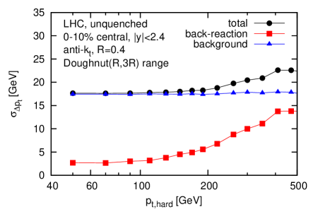
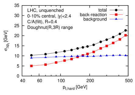
Figure 16: The decomposition of the dispersion into back-reaction and “background” components (including misestimation of $\rho$). The left-hand plot is for the anti-$k_{t}$ algorithm and the right-hand one for C/A(filt). Both correspond to LHC collisions at $\sqrt{s_{NN}}=5.5\,\mathrm{TeV}$.

We stated, in section 4.3.2, that the increase of the dispersion at high $p_{t}$ seen in fig. 8 was mainly due to back-reaction. This is made explicit in fig. 16, which decomposes the dispersion into its two components: that associated with the back-reaction, $\sigma_{\Delta p_{t}}^{\mathrm{BR}}$ and that associated with background fluctuations and misestimation of $\rho$ (defined as $[\sigma_{\Delta p_{t}}^{2}-(\sigma_{\Delta p_{t}}^{\mathrm{BR}})^{2}]^{\frac{1}{2}}$). One sees that the background-fluctuation component is essentially independent of $p_{t}$, while the back-reaction dispersion has a noticeable $p_{t}$ dependence. This is the case because the back-reaction dispersion is dominated by rare events in which two similarly hard subjets are separated by a distance close to $R$ (specifically by $R+\epsilon$ with $\epsilon\ll 1$). In such a configuration, the background’s contribution to the two subjets can affect whether they recombine and so lead to a large, ${\cal{O}}\left(p_{t}\right)$, change to the jet’s momentum. In the limit of a uniform background, $\sigma/\rho\ll 1$, this can be shown to occur with a probability of order $\alpha_{s}\rho R^{2}/p_{t}$. Thus the contribution to the average shift $\left\langle\Delta p_{t}\right\rangle$ is proportional to $\alpha_{s}\rho R^{2}$ (which in a full analysis is found to be enhanced by a logarithm [15] for the $k_{t}$ and C/A algorithms), while the contribution to $\left\langle\Delta p_{t}^{2}\right\rangle$ goes as $\alpha_{s}\rho R^{2}p_{t}$, and so leads to a dispersion that should grow asymptotically as $\sqrt{p_{t}}$ (fig. 16 is, however, probably not yet in the asymptotic regime).

It is worth keeping in mind that even though rare but large back-reaction dominates the overall dispersion, it will probably not be the main contributor in distorting the reconstructed jet spectrum. Such distortions come from upwards $\Delta p_{t}$ fluctuations, whereas large back-reaction tends to be dominated by downwards fluctuations. The reason is simple: in order to have an upwards fluctuation from back-reaction, there must be extra $p_{t}$ near the jet in the original $pp$ event. This implies the presence of a harder underlying $2\to 2$ scattering than would be deduced from the jet $p_{t}$, with a corresponding significant price to pay in terms of more suppressed matrix elements and PDFs.

Figure 16 also shows that the non-back-reaction component is nearly independent of $p_{t}$. This is expected since the anomalous dimension of the jet area is zero for anti-$k_{t}$ and small for C/A (with or without filtering), and in any case leads to a weak scaling with $p_{t}$, as $\ln\ln p_{t}$. Furthermore, there is roughly a factor of $1/\sqrt{2}$ between anti-$k_{t}$ and C/A(filt), as expected based on a proportionality of the dispersion to the square-root of the jet area.

C.2 Quality of area determination

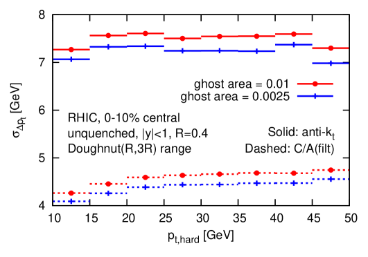
Figure 17: Dispersion, $\sigma_{\Delta p_{t}}$, for RHIC, as a function of the jet $p_{t}$, with two different choices for the ghost area, $0.01$ and $0.0025$.

One further source of $\Delta p_{t}$ fluctuations can come from imperfect estimation of the area of the jets. We recall that throughout this article we have used soft ghosts, each with area of $0.01$, in order to establish the jet area. That implies a corresponding finite resolution on the jet area and related poor estimation of the exact edges of the jets, which can have an impact on the amount of background that one subtracts from each jet, and, consequently, on the final dispersion. It is therefore interesting to see, figure 17, that the dispersion $\sigma_{\Delta p_{t}}$ is reduced by about $0.2-0.4\,\mathrm{GeV}$ if one lowers the ghost area to $0.0025$.

While this doesn’t affect any of the conclusions of our paper, it does suggest that for a full experimental analysis there are benefits to be had from using a ghost area that is smaller than the default FastJet setting of $0.01$.

References

- [1] S. Catani, Y. L. Dokshitzer, M. H. Seymour, and B. R. Webber, Nucl. Phys. B406 (1993) 187; S. Catani, Y. L. Dokshitzer, M. Olsson, G. Turnock, and B. R. Webber, Phys. Lett. B269 (1991) 432; S. D. Ellis and D. E. Soper, Phys. Rev. D48 (1993) 3160–3166, [hep-ph/9305266].
- [2] Y. L. Dokshitzer, G. D. Leder, S. Moretti, and B. R. Webber, JHEP 08 (1997) 001, [hep-ph/9707323]; M. Wobisch and T. Wengler, hep-ph/9907280.
- [3] M. Cacciari, G. P. Salam and G. Soyez, JHEP 0804 (2008) 063 [arXiv:0802.1189].
- [4] G. P. Salam and G. Soyez, JHEP 05 (2007) 086, [arXiv:0704.0292]; see also, http://projects.hepforge.org/siscone.
- [5] O.L. Kodolova et al, “Study of +Jet Channel in Heavy ion Collisions with CMS,” CMS NOTE-1998/063. V. Gavrilov, A. Oulianov, O. Kodolova and I. Vardanian, “Jet Reconstruction with Pileup Subtraction,” CMS RN 2003/004.
- [6] S. L. Blyth et al., J. Phys. G 34 (2007) 271 [nucl-ex/0609023].
- [7] N. Grau for the ATLAS Collaboration, J. Phys. G 35 (2008) 104040 [arXiv:0805.4656].
- [8] S. Salur [STAR Collaboration], Eur. Phys. J. C 61 (2009) 761 [arXiv:0809.1609].
- [9] Y. -S. Lai, B. A. Cole, [arXiv:0806.1499].
- [10] N. Grau, B. A. Cole, W. G. Holzmann, M. Spousta and P. Steinberg [ATLAS Collaboration], Eur. Phys. J. C 62 (2009) 191 [arXiv:0810.1219].
- [11] Y. S. Lai for the PHENIX collaboration, arXiv:0911.3399.
- [12] M. Estienne [ALICE Collaboration], arXiv:0910.2482.
- [13] J. Kapitan, arXiv:0911.4754.
- [14] M. Cacciari and G. P. Salam, Phys. Lett. B 659 (2008) 119 [arXiv:0707.1378].
- [15] M. Cacciari, G. P. Salam and G. Soyez, JHEP 0804 (2008) 005 [arXiv:0802.1188].
- [16] M. Cacciari, G. P. Salam and S. Sapeta, JHEP 1004, 065 (2010) [arXiv:0912.4926].
- [17] M. Cacciari, J. Rojo, G. P. Salam and G. Soyez, JHEP 0812 (2008) 032 [arXiv:0810.1304]; see also http://quality.fastjet.fr.
- [18] S. Salur, Nucl. Phys. A 830 (2009) 139C [arXiv:0907.4536]; M. Ploskon [STAR Collaboration], Nucl. Phys. A 830 (2009) 255C [arXiv:0908.1799].
- [19] I. P. Lokhtin and A. M. Snigirev, Eur. Phys. J. C 45 (2006) 211 [arXiv:hep-ph/0506189].
- [20] I. P. Lokhtin, L. V. Malinina, S. V. Petrushanko, A. M. Snigirev, I. Arsene and K. Tywoniuk, Comput. Phys. Commun. 180 (2009) 779 [arXiv:0809.2708].
- [21] R. Baier, Y. L. Dokshitzer, A. H. Mueller, S. Peigne and D. Schiff, Nucl. Phys. B 484 (1997) 265 [hep-ph/9608322]; B. G. Zakharov, JETP Lett. 65 (1997) 615 [hep-ph/9704255].
- [22] J. Casalderrey-Solana and C. A. Salgado, Acta Phys. Polon. B 38 (2007) 3731 [arXiv:0712.3443]; D. d’Enterria, arXiv:0902.2011; U. A. Wiedemann, arXiv:0908.2306; A. Majumder and M. Van Leeuwen, arXiv:1002.2206; D. d’Enterria and B. Betz, Lect. Notes Phys. 785 (2010) 285.
- [23] T. Sjostrand, S. Mrenna and P. Skands, JHEP05 (2006) 026 [hep-ph/0603175].
- [24] N. Armesto, L. Cunqueiro and C. A. Salgado, Eur. Phys. J. C 63 (2009) 679 [arXiv:0907.1014]; N. Armesto, L. Cunqueiro, C. A. Salgado and W. C. Xiang, JHEP 0802 (2008) 048 [arXiv:0710.3073].
- [25] M. Cacciari and G. P. Salam, Phys. Lett. B 641 (2006) 57 [hep-ph/0512210].
- [26] J. M. Butterworth, A. R. Davison, M. Rubin and G. P. Salam, Phys. Rev. Lett. 100 (2008) 242001 [arXiv:0802.2470].
- [27] D. Krohn, J. Thaler and L. T. Wang, JHEP 1002 (2010) 084 [arXiv:0912.1342].
- [28] S. D. Ellis, C. K. Vermilion and J. R. Walsh, Phys. Rev. D 81 (2010) 094023 [arXiv:0912.0033].
- [29] M. Cacciari, G. P. Salam and G. Soyez, http://www.fastjet.fr.
- [30] J. Adams et al. [STAR Collaboration], Phys. Rev. C 70 (2004) 054907 [nucl-ex/0407003].
- [31] S. S. Adler et al. [PHENIX Collaboration], Phys. Rev. C 71 (2005) 034908 [Erratum-ibid. C 71 (2005) 049901] [nucl-ex/0409015].
- [32] B. B. Back et al., Phys. Rev. Lett. 91 (2003) 052303 [nucl-ex/0210015].
- [33] B. B. Back et al. [PHOBOS Collaboration], Phys. Lett. B578 (2004) 297-303. [nucl-ex/0302015].
- [34] A. Adare et al. [PHENIX Collaboration], Phys. Rev. Lett. 101 (2008) 232301. [arXiv:0801.4020].
- [35] N. Armesto, arXiv:0903.1330 [hep-ph].
- [36] S. S. Adler et al. [PHENIX Collaboration], Phys. Rev. Lett. 91 (2003) 182301 [nucl-ex/0305013]; J. Adams et al. [STAR Collaboration], Phys. Rev. Lett. 92 (2004) 052302 [nucl-ex/0306007]; C. Alt et al. [NA49 Collaboration], Phys. Rev. C 68 (2003) 034903 [nucl-ex/0303001]; B. B. Back et al. [PHOBOS Collaboration], Phys. Rev. C 72 (2005) 051901 [nucl-ex/0407012].
- [37] J. Y. Ollitrault, Phys. Rev. D 46 (1992) 229; A. M. Poskanzer and S. A. Voloshin, Phys. Rev. C 58 (1998) 1671 [nucl-ex/9805001].
- [38] I. P. Lokhtin and A. M. Snigirev, hep-ph/0312204.
- [39] K. Zapp, G. Ingelman, J. Rathsman, J. Stachel and U. A. Wiedemann, Eur. Phys. J. C 60 (2009) 617 [arXiv:0804.3568].
- [40] B. Schenke, C. Gale and S. Jeon, Phys. Rev. C 80 (2009) 054913 [arXiv:0909.2037].
- [41] P. Jacobs, presentation at “Jets in p+p and heavy-ion collisions,” Prague, August 12-14, 2010, http://bazille.fjfi.cvut.cz/~jetworkshop/talkdir/peter_jacobs.pdf
- [42] E. Bruna for the STAR Collaboration, presentation at “Jets in p+p and heavy-ion collisions,” Prague, August 12-14, 2010, http://bazille.fjfi.cvut.cz/~jetworkshop/talkdir/elena_bruna.ppt.