Linear noise approximation of noise-induced oscillation in NF-$\kappa$B signaling network

Abstract

NF-$\kappa$B, one of key regulators of inflammation, apoptosis, and differentiation, was found to have noisy oscillatory shuttling between the nucleus and the cytoplasm in single cells when cells are stimulated by cytokine TNF$\alpha$. We present the analytical analysis which uncovers the underlying physical mechanisms of this spectacular noise-induced transition in biological networks. Starting with the master equation describing both signaling and transcription events in NF-$\kappa$B signaling network, we derived the macroscopic and the Fokker-Planck equations by using van Kampen’s sysem size expansion. Using the noise-induced oscillatory signatures present in the power spectrum, we constructed the two-dimensional phase diagram where the noise-iduced oscillation emerges in the dynamically stable parameter space.

1 Introduction

Oscillations are prevalent in biology. Neurons periodically fire pulses, cells undergo cell-cycle, and living organisms maintain their internal biological clock of about 24 hours (Murray 1980). Strikingly, live cell imaging techniques revealed that biochemical reactions are likely to exhibit oscillatory behavior in single cells. For example, perpetual oscillations of a tumor suppressor protein p53 and its suppressor mdm2 have been observed in single cells when cells were exposed to ionizing UV irradiation (Lahav et al 2004). In addition, NF-$\kappa$B, one of key regulators of inflammation, apoptosis, and differentiation, was found to shuttle between the nucleus and the cytoplasm of single cells when cells are stimulated by cytokine TNF$\alpha$ (Nelson et al 2004). Despite its universal appearance and its potential biological functions, the underlying physical mechanisms of such biological oscillations in noisy cellular environments have been neither discussed nor investigated to a mathematically satisfactory degree. Sadly, most of publicly available investigations on the subject are based on numerical simulations and are quite limited in providing physical and mathematical insights behind these fascinating natural phenomena. In this manuscript, we’d like to present the analytical analysis which uncovers the underlying mechanisms of the spectacular noise-induced transition in one of biochemical oscillations.

In biological, physical,and chemical systems, stochastic fluctuations (white noise) can induce oscillations in a dynamical system with an external periodic forcing (Steuer 2004; Pikovsky et al 1997; Neiman et al 1997; Gammaitoni et al 1998; Benzi et al 1982). This phenomena are called stochastic resonance where the background white noise amplifies the external periodic input signal and such an amplification is optimized at an intermediate level of noise. On the other hand, noise can also coherently induce oscillations without external periodic modulation. In this case the deterministic dynamical system has a stable fixed point, but has a long excursion in phase trajectory because of nearby dynamical instability; the system is constantly kicked off a stable fixed point by stochastic fluctuations and follows a deterministic phase trajectory at the natural frequency at which the system reaches its stable fixed point. This coherent noise-induced oscillation (NIO) was investigated in several model systems (Wiesenfeld 1985; Gang et al 1993; Mckane & Newman 2007). In addition, researchers revisited the previous studies of biological oscillations and investigated the effects of noise on the existence & emergence of limit cycles. The deterministic limit cycle emerges at some confined parameter space whereas stochastic fluctuations increase such a domain where noise not only stabilizes the limit cycle, but also induces oscillations at a parameter space where the deterministic dynamics produces a stable dynamics.

We are interested in the effects of noise on the stable dynamics generated by negative feedback loops that are most commonly found in the biological networks. In the recent paper (Joo et al 2010), the authors presented NIO dynamic phenomena on a large-scale signal transduction network of NF-$\kappa$B. A full stochastic two-compartmental model of the NF-$\kappa$B signal transduction network consisting of 28 biochemical species and 71 kinetic parameters was investigated with the help of Gillespie stochastic simulations and, depending on the choice of the kinetic parameter values, yielded a phase diagram consisting of oscillations and damped-oscillations of NF-$\kappa$B shuttling in carefully chosen two-dimensional parameter space. The authors successfully demonstrated the noise-induced oscillations of the NF-$\kappa$B shuttling and identified the inherent stochastic fluctuations as the potential source of those fantastic stochastic phenomena. However, the full scale stochastic simulations with the large-scale size network and its nonlinear complexity, put a hard limit on our capability in investigating the characteristics of the bifurcation, the dependence of the NIO on the remaining parameter space. What is worse, the numerical analysis suffers from the lack of kinetic details, e.g., functional forms of reactions and associated kinetic parameter values. Thus, to overcome the difficulties described above, we like to perform stochastic analysis of a reduced network of NF-$\kappa$B, assuming a linear response of the system to small perturbation

In this paper, using the stochastic reduced order model of NF-$\kappa$B signaling network and linear noise approximation, we present the underlying physical mechanisms of the NIO and show analytically the emergence of the NIO. We took into account the full stochastic nature of transcriptional processes in the model. We started with the master equation describing both signaling and transcription events, and then derived the macroscopic and Fokker-Planck equations by using van Kampen’s sysem size expansion. First, we performed linear stability analysis of macroscopic equations. Second, using the NIO signatures present in the power spectrum derived from Langevin equations, we constructed the two-dimensional phase diagram where the NIO emerges in the dynamically stable parameter space.

2 Model description

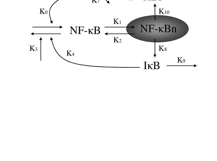
Figure 1: Minimal model consisting of five proteins, IKK, cytoplasmic NF-$\kappa$B (NF-$\kappa$B), nuclear NF-$\kappa$B (NF-$\kappa$Bn), I$\kappa$B, and A20. The synthesis of both A20 and I$\kappa$B depends on the NF-$\kappa$Bn. $K$’s denote the reaction rates of the respective reactions. The external signal is received from the $K_{6}$.

The full network consisting of 28 species and 71 kinetic parameters can be topologically reduced to an intermediately reduced network consisting of seven components, by using sensitivity analysis that calculates the correlation coefficients between kinetic parameters and the NF-$\kappa$B dynamic response and eliminates insignificant kinetic parameters whose change doesn’t significantly affect the NF-$\kappa$B response as presented in Ref. (Joo et al 2007). We further eliminate two fast variables, mRNA I$\kappa$B and mRNA A20, whose half life are less than a half hour, obtaining a reduced network as shown in Fig. 1.

In more rigorous study of the stochastic dynamical system, one should start with a stochastic model of full NF-$\kappa$B signaling network and adiabatically eliminate the ”fast varying variables”. However, the adiabatic elimination of the fast varying variables from the Makovian stochastic system leads to non-Markovian system, making analysis almost impossible and thus adiabatic elimination techniques are limited only to a small stochastic system. Thus, we take an non-rigorous but practical way of model reduction; we reduce the complexity or the dimension of the NF-$\kappa$B signaling network by using various heuristic techniques and then the reduced network is converted to a stochastic minimal model.

The current stochastic model neglects an intermediate step of protein synthesis, namely mRNA, that a typical stochastic model with modest level of complexity always contains. But, the mRNA and protein synthesis processes are too complicated to model them with a finite number of steps. Thus, we simply represent them with a single step (a single variable). Lastly, we include the stochastic fluctuations in DNA and protein NF-$\kappa$ interaction.

The dynamic system under our consideration regulates the shuttling dynamics of NF-$\kappa$B protein between cytoplasm and nucleus. In the absence of stimulus, the activated IKK is absent and NF-$\kappa$B can exist either in a free form (NF-$\kappa$B) or can be bound with inhibitor $\kappa$B, forming a complex (I$\kappa$B:NF-$\kappa$B). The total amount of NF-$\kappa$B, $X_{o}$, is conserved, enabling us to omit the expression of a protein complex I$\kappa$B:NF-$\kappa$B from our model because the amount of protein complex I$\kappa$B:NF-$\kappa$B is simply $X_{o}$-NF-$\kappa$ B. The free NF-$\kappa$B can enter into nucleus with a rate $k_{1}$ or moves out of nucleus with a rate $k_{2}$ by nuclear transport proteins. The liberated & translocated NF-$\kappa$B into nucleus initiates mRNA & protein syntheses of I$\kappa$B and A20 with rates $k_{8}$ and $k_{10}$ respectively, both of which forms negative feedback loops, negatively regulating the translocation of NF-$\kappa$B into nucleus. The newly synthesized I$\kappa$B bind to NF-$\kappa$B with a rate $k_{4}$, forming a protein complex I$\kappa$B-NF-$\kappa$B. Upon stimulus, I$\kappa$B kinase (IKK) is activated with a constant rate, $S\cdot k_{6}$ where $S$ is stimulus strength and also is deactivated with a rate $k_{7}$. This IKK induces I$\kappa$B decay from I$\kappa$B-NF-$\kappa$B and liberates NF-$\kappa$B with a rate $k_{o}$, which translocates NF-$\kappa$B into nucleus, increasing the synthesis of negative regulators I$\kappa$B and A20. In turn, A20 inactivates the activated IKK with a rate $k_{5}$. A20 and I$\kappa$B also decay with rates $k_{9}$ and $k_{11}$ respectively.

3 Derivation of chemical master equation

We intend to use a probabilistic model of the NF-$\kappa$B system to be able to capture unusual stochastic phenomena such as noise-amplified oscillation. Let us define the joint probability density $P_{t}(\underline{\eta})$denoting the probability of the system to be in a state $\underline{\eta}(t)=(C_{t},D_{t},X_{t},Y_{t},Z_{t})$ at time $t$ where $C_{t}$, $D_{t}$, $X_{t}$, $Y_{t}$, and $Z_{t}$ denote the molecule number of $I\kappa B$, A20, NF-$\kappa$B, $NF\kappa Bn$, and IKK proteins at time $t$, respectively. The time evolution of the joint probability is determined by the transition probability per unit time $T(\underline{\eta}|\underline{\eta^{\prime}};t)$ of going from a state $\underline{\eta}$ to a state $\underline{\eta^{\prime}}$. We assume that the transition probabilites do not depend on the history of the previous states of the system but only on the immediately past state. There are only a few transitions that are allowed to take place and their transition rates are

$$T_{0}(...,X_{t},...|...,X_{t}+1,...;t) = k_{o}\Omega_{C}(\frac{X_{o}-X_{t}-Y_{t}}{\Omega_{C}})(\frac{Z_{t}}{\Omega_{C}}),$$ (1)

$$T_{1}(...,X_{t},Y_{t},...|...,X_{t}-1,Y_{t}+1,...;t) = k_{1}\Omega_{C}(\frac{X_{t}}{\Omega_{C}}),$$

$$T_{2}(...,X_{t},Y_{t},...|...,X_{t}+1,Y_{t}-1,...;t) = k_{2}\Omega_{N}(\frac{Y_{t}}{\Omega_{N}}),$$

$$T_{3}(...,X_{t},...|...,X_{t}-1,...;t) = k_{3}\Omega_{C}(\frac{X_{t}}{\Omega_{C}}),$$

$$T_{4}(C_{t},...,X_{t},...|C_{t},...,X_{t}-1,...;t) = k_{4}\Omega_{C}(\frac{X_{t}}{\Omega_{C}})(\frac{C_{t}}{\Omega_{C}}),$$

$$T_{5}(...,D_{t},...,Z_{t}|...,D_{t},...,Z_{t}-1;t) = k_{5}\Omega_{C}(\frac{D_{t}}{\Omega_{C}}(\frac{Z_{t}}{\Omega_{C}}),$$

$$T_{6}(...,Z_{t}|...,Z_{t}+1;t) = k_{6}S\Omega_{C},$$

$$T_{7}(...,Z_{t}|...,Z_{t}-1;t) = k_{7}\Omega_{C}(\frac{Z_{t}}{\Omega_{C}}),$$

$$T_{8}(C_{t},...,Y_{t},...|C_{t}+1,...,Y_{t},...;t) = k_{8}\Omega_{C}(\frac{Y_{t}}{\Omega_{N}}),$$

$$T_{9}(C_{t},...|C_{t}-1,...) = k_{9}\Omega_{C}(\frac{C_{t}}{\Omega_{C}}),$$

$$T_{10}(...,D_{t},...,Y_{t},...|...,D_{t}+1,...,Y_{t},...;t) = k_{10}\Omega_{C}(\frac{Y_{t}}{\Omega_{N}}),$$

$$T_{11}(...,D_{t},...|...,D_{t}-1,...;t) = k_{11}\Omega_{C}(\frac{D_{t}}{\Omega_{C}})$$

where $\Omega_{C}$ and $\Omega_{N}$ are the cytoplasmic and nuclear volumes of a typical cell, respectively. $X_{o}$ is an initial and conserved molecule number of NF-$\kappa B$ protein. The above transition rates are provided as defined in Ref. (van Kampen 2001) and given in three terms in the following order: a reaction rate, a reactive volume where the reaction takes place, and the concentration(s) of all involved components, e.g., $k_{1}\cdot\Omega_{C}\cdot\frac{X_{t}}{\Omega_{C}}$. All the above transitions occur at the cytoplasm except the transition $T_{2}$. The transition $T_{2}$ (or $T_{1}$) describes a binary (associative) reaction between a NF-$\kappa$B protein in nucleus (or in cytoplasm) and a transport protein called “exportin” present in nucleus (or “importin” present in cytoplasm), leading to the transportation of NF-$\kappa$B protein into cytoplasm (or into nucleus). The reactive volume is thus nuclear volume $\Omega_{N}$ (or cytoplasmic volume $\Omega_{C}$) and assuming a constant concentration of importin and exportin being independent of the system’s variables, their concentrations are absorbed into reaction rates. Two transitions, $T_{8}$ and $T_{10}$, describe a complex mRNA and protein synthesis in a single term and those syntheses begin from the reaction between nuclear NF-$\kappa$B and DNA in nucleus and ends at the production of a protein out of Ribosome in cytoplasm. Thus, the reactive volume of these two transitions is the cytoplasmic volume. In fact, these two transitions oversimplify very stochastic nature of transcription and translation. A more realistic model is provided and analyzed in appendix A.

The stochastic process specified by the transition rates in Eq. (1) is Markovian, thus we can immediately write down a master equation governing the time evolution of the joint probability $P_{t}(\underline{\eta})$. The rate of change of the joint probability $P_{t}(\underline{\eta})$ is the sum of transition rates from all other states $\underline{\eta^{\prime}}$ to the state $\underline{\eta}$, minus the sum of transition rates from the state $\underline{\eta}$ to all other states $\underline{\eta^{\prime}}$:

$$\frac{dP_{t}(\underline{\eta})}{dt} = (E^{-1}_{X}-1)T_{0}(...,X_{t},...|...,X_{t}+1,...;t)P_{t}(\underline{\eta})$$

$$+ (E_{X}E^{-1}_{Y}-1)T_{1}(...,X_{t},Y_{t},...|...,X_{t}-1,Y_{t}+1,...;t)P_{t}(\underline{\eta})$$

$$+ (E^{-1}_{X}E_{Y}-1)T_{2}(...,X_{t},Y_{t},...|...,X_{t}+1,Y_{t}-1,...;t)P_{t}(\underline{\eta})$$

$$+ (E_{X}-1)T_{3}(...,X_{t},...|...,X_{t}-1,...;t)P_{t}(\underline{\eta})$$

$$+ (E_{X}E_{C}-1)T_{4}(C_{t},...,X_{t},...|C_{t}-1,...,X_{t}-1,...;t)P_{t}(\underline{\eta})$$

$$+ (E_{Z}-1)T_{5}(...,D_{t},...,Z_{t}|...,D_{t},...,Z_{t}-1;t)P_{t}(\underline{\eta})$$

$$+ (E^{-1}_{Z}-1)T_{6}(...,Z_{t}|...,Z_{t}+1;t)P_{t}(\underline{\eta})$$

$$+ (E_{Z}-1)T_{7}(...,Z_{t}|...,Z_{t}-1;t)P_{t}(\underline{\eta})$$

$$+ (E^{-1}_{C}-1)T_{8}(C_{t},...,Y_{t},...|C_{t}+1,...,Y_{t},...;t)P_{t}(\underline{\eta})$$

$$+ (E_{C}-1)T_{9}(C_{t},...|C_{t}-1,...)P_{t}(\underline{\eta})$$

$$+ (E^{-1}_{D}-1)T_{10}(...,D_{t},...,Y_{t},...|...,D_{t}+1,...,Y_{t},...;t)P_{t}(\underline{\eta})$$

$$+ (E_{D}-1)T_{11}(...,D_{t},...|...,D_{t}-1,...;t)P_{t}(\underline{\eta})$$

where $E^{\pm}_{\alpha}$ is a step operator which acts on any function of $\alpha$ according to $E^{\pm}_{\alpha}f(\alpha\pm 1,...)=f(\alpha\pm 1,...)$.

4 System size expansion of the chemical master equation

In this section we will apply van Kampen’s elegant “system size $\Omega$-expansion method” to the chemical master equation in Eq. (3). This van kampen’s $\Omega$-expansion method not only allows us to obtain a deterministic version of the stochastic model in Eq. (3) but also enables us to find Gaussian corrections to the deterministic result. We choose two system sizes, cytoplasmic volume $\Omega_{C}$ and nuclear volume $\Omega_{N}$, and expand the master equation in order of $\Omega^{1/2}_{C}$ and $\Omega^{1/2}_{N}$. A required condition for valid use of $\Omega$-expansion is the stability of fixed points and restricts us to perform this analysis only inside of the dynamically stable region.

For large and finite cytoplasmic and nuclear volume, $\Omega_{C}$ and $\Omega_{N}$, we would expect $P(\underline{\eta})$ to have a finite width of order $\Omega^{1/2}$. The variables (X, Y, C, D, Z) are stochastic and we introduce new stochastic variables ($\xi_{X}$, $\xi_{Y}$, $\xi_{C}$, $\xi_{D}$, $\xi_{Z}$): $X=x\Omega_{C}+\sqrt{\Omega_{C}}\xi_{X}$, $Y=y\Omega_{N}+\sqrt{\Omega_{N}}\xi_{Y}$, $C=c\Omega_{C}+\sqrt{\Omega_{C}}\xi_{C}$, $D=d\Omega_{C}+\sqrt{\Omega_{C}}\xi_{D}$, and $Z=z\Omega_{C}+\sqrt{\Omega_{C}}\xi_{Z}$. These new stochastic variables represent inherent noise contribute to deviation of the system from the macroscopic dynamical behavior.

The new joint probability density function $\Pi_{t}$ is defined by $\Pi_{t}(\underline{\xi})\equiv P_{t}(\underline{\eta})$. Let us define the step operators $E^{\pm}_{\alpha}$ which change the state $\alpha$ to $\alpha+1$ and therefore $\xi_{\alpha}$ into $\xi_{\alpha}+\Omega^{1/2}$, so that the continuous approximation of the step operator is

$$E^{\pm}_{\alpha}=1\pm\Omega^{-\frac{1}{2}}\frac{\partial}{\partial\xi_{\alpha}}+\frac{\Omega^{-1}}{2}\frac{\partial^{2}}{\partial\xi^{2}_{\alpha}}\pm...$$ (3)

where $\Omega$ becomes $\Omega_{C}$ for cytoplasmic component $\alpha$ and $\Omega_{N}$ for nucleoplasmic $\alpha$. The time derivative of the the joint probability $P_{t}(\underline{\eta})$ in Eq. (3) is taken at a fixed state $\underline{\eta}$, which implies that the time-derivative on both sides of $\alpha=\Omega\alpha+\Omega^{1/2}\xi_{\alpha}$ should lead to $d\xi_{\alpha}/dt=-\Omega^{1/2}$ $d\alpha/dt$. Therefore,

$$\frac{dP_{t}(\underline{\eta})}{dt}=\frac{\partial\Pi_{t}(\underline{\xi})}{\partial t}-\sum_{\alpha=X,C,D,Z}\{\Omega^{1/2}_{C}\frac{d\alpha}{dt}\frac{\partial\Pi_{t}(\underline{\xi})}{\partial\xi_{\alpha}}\}-\Omega^{1/2}_{N}\frac{dy}{dt}\frac{\partial\Pi_{t}(\underline{\xi})}{\partial\xi_{Y}}$$ (4)

The initial condition for the above parabolic PDE is $P_{t=0}(\underline{\eta})=\delta_{\underline{\eta},\underline{\eta_{0}}}$. When the Eq. (3) is expanded in order of $\Omega^{1/2}_{C}$ and $\Omega^{1/2}_{N}$, we can collect several powers of $\Omega^{1/2}_{C}$ and $\Omega^{1/2}_{N}$. The macroscopic equations emerge from the terms of order $\Omega^{1/2}_{C}$ and $\Omega^{1/2}_{N}$ and the linear Fokker-Planck equation is obtained from the terms of order $\Omega^{0}_{C}$ and $\Omega^{0}_{N}$.

5 Emergence of the macroscopic equations

By matching the terms in order of $\Omega^{1/2}$ in Eqs. (3) and  (4), we can identify the macroscopic equations as follows:

$$\frac{dx(t)}{dt} = k_{0}(x_{0}-x(t)-y(t)/K_{v})z_{t}-k_{1}x(t)+k_{2}y(t)/K_{v}-k_{3}x(t)-k_{4}c(t)x(t)$$ (5)

$$\frac{dy(t)}{dt} = k_{1}x(t)K_{v}-k_{2}y(t)$$

$$\frac{dc(t)}{dt} = k_{8}y(t)-k_{9}c(t)-k_{4}c(t)x(t)$$

$$\frac{dd(t)}{dt} = k_{10}y(t)-k_{11}d(t)$$

$$\frac{dz(t)}{dt} = S\cdot k_{6}-k_{7}z(t)-k_{5}d(t)z(t)$$

The above macroscopic equations are nothing but the deterministic equations of the corresponding stochastic model in the limit of infinitely large $\Omega$, i.e., in the limit of negligible fluctuations.

The steady state solutions of the macroscopic equations can be obtained by setting the left-handed sides of the Eq. (5): $\bar{y}=k_{1}K_{v}\bar{x}/k_{2}$, $\bar{c}=k_{1}k_{8}K_{v}\bar{x}/(k_{2}k_{9})$, $\bar{z}=k_{6}S/(k_{7}+k_{1}k_{5}k_{10}K_{v}\bar{x}/(k_{2}k_{11}))$. The steady state solutions of $\bar{x}$ are the roots of the cubic equation, i.e., $dx_{t}/dt=0$ and only one of three roots are positive real number and biologically feasible solution. We perform a linear stability analysis by small perturbation of the dynamic system from the feasible steady state solution, i.e., $\delta\vec{x}(t)\equiv\vec{x}(t)-\bar{\vec{x}}$. We rewrite the Eq. 5 in terms of this vector $\delta\vec{x}(t)$: $d\delta\vec{x}(t)/dt=M\cdot\delta\vec{x}(t)$. The stability of the steady state of the Eq. (5) is solely determined by the Jacobian matrix $M$:
$M=\left(\begin{array}[]{ccccc}M_{11}&M_{12}&M_{13}&0&M_{15}\\ M_{21}&M_{22}&0&0&0\\ M_{31}&M_{32}&M_{33}&0&0\\ 0&M_{42}&0&M_{44}&0\\ 0&0&&M_{54}&M_{55}\end{array}\right)$
where $M_{11}=-k_{0}\bar{z}-k_{1}-k_{3}-k_{4}\bar{c}$, $M_{12}=(k_{2}-k_{0}\bar{z})/\sqrt{K_{v}}$, $M_{13}=-k_{4}\bar{x}$, $M_{15}=k_{o}(x_{0}-\bar{x}-\bar{y}/K_{v})$, $M_{21}=k_{1}\sqrt{K_{v}}$, $M_{22}=-k_{2}$, $M_{31}=-k_{4}\bar{c}$, $M_{32}=k_{8}\sqrt{K_{v}}$, $M_{33}=-k_{4}\bar{x}-k_{9}$, $M_{42}=k_{10}\sqrt{K_{v}}$, $M_{44}=-k_{11}$, $M_{54}=-k_{5}\bar{z}$, $M_{55}=-k_{5}\bar{d}-k_{7}$.

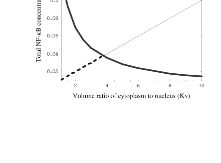
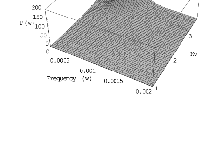
Figure 2: Phase diagram of NF-$\kappa$ oscillation on two model parameter space, the volume ratio of cytoplasm to nucleus (Kv) and the total NFKB concetration, for the wild type case. (A) shows the deterministic dynamical instability region where the fixed point of the macroscopic equations is unstable due to the Hopf bifurcation. (B) shows the power spectra in subcritical region along the diagonal direction as indicated as the dashed line in (A). (B) shows the power spectra at fixed value of Kv=2.5 in subcritical region.

The characteristic equation $|M-E\lambda|$ is the fifth order polynomial equation and thus has five roots. The steady state of the dynamical system is stable when the real parts of all the roots are negative. Now for the macroscopic equations in Eq. (5), the three roots are always negative real numbers within the biologically feasible domain of the kinetic parameters under our consideration whereas the other two roots form a pair of complex conjugate whose real part undergoes a sign change as a function of the kinetic parameters. Thus, oscillation of this NF-$\kappa$B signaling network arise from Hopf bifurcation mechanism. A two-variable bifurcation diagram shown in Fig. 2(A) is constructed by numerically solving the characteristic equation. When both total NF-$\kappa$B concentration and volume ratio of cytoplasm to nucleoplasm increases along the diagonal direction in Fig. 2(A), the real parts of two complex conjugate roots are changed from negative to positive values and the onset of the Hopf bifurcation takes place at $Kv^{Hopf}=3.754...$, giving rise to the emergence of a limit cycle.

6 A linear Fokker-Planck Equation

The next-to-leading order terms, $\Omega^{0}$, in the power expansion of the master equation, give a partial differential equation for the time evolution of the probability distribution $\Pi_{t}(\underline{\xi})$, which has the form

$$\frac{\partial\Pi_{t}}{\partial t}=-\sum_{\alpha}\frac{\partial A_{\alpha}(\underline{\xi})\Pi_{t}}{\partial\xi_{\alpha}}+\frac{1}{2}\sum_{\alpha\beta}B_{\alpha\beta}\frac{\partial^{2}\Pi_{t}}{\partial\xi_{\alpha}\partial\xi_{\beta}}$$ (6)

where $A_{\alpha}(\underline{\xi})=\sum_{\beta}M_{\alpha\beta}\xi_{\beta}$, $\alpha=X,Y,C,D,Z$, and $M$ is a Jacobian marix of the Eq. (5) and $B$ are provided as below:
$B=\left(\begin{array}[]{ccccc}B_{11}&B_{12}&B_{13}&0&0\\ B_{21}&B_{22}&0&0&0\\ B_{31}&0&B_{33}&0&0\\ 0&0&0&B_{44}&0\\ 0&0&&0&B_{55}\end{array}\right)$
where the elements of both matrices $M$ and $B$ are fully determined by the steady state solution of the macroscopic equations, denoted by $\bar{\alpha}$: $B_{11}=k_{o}\bar{z}(x_{0}-\bar{x}-\bar{y}/K_{v})+k_{1}\bar{x}+k_{2}\bar{y}/K_{v}+k_{3}\bar{x}+k_{4}\bar{x}\bar{c}$, $B_{12}=B_{21}=-2k_{1}\sqrt{K_{v}}\bar{x}-2k_{2}\bar{y}/\sqrt{K_{v}}$, $B_{13}=B_{31}=2k_{4}\bar{x}\bar{c}$, $B_{22}=k_{2}\bar{y}+k_{1}\bar{x}K_{v}$, $B_{33}=k_{4}\bar{x}\bar{c}+k_{8}\bar{y}+k_{9}\bar{c}$, $B_{44}=k_{10}\bar{y}+k_{11}\bar{d}$, $B_{55}=k_{5}\bar{d}\bar{z}+k_{6}S+k_{7}\bar{z}$.

The probability distribution at next-to-leading order is completely determined by two $5\times 5$ matrices. $A_{\alpha}(\xi)$ remain linear functions of the $\xi_{\beta}$ and the $B_{\alpha\beta}$ remain independent of them. Even though it is a characteristic of a large $\Omega$ expansion for a single compartmental model that $M$ is the Jacobian matrix which determines the stability at a fixed point. The partial differential equation is a linear Fokker-Planck equation, a continuous version of the master equation and can be solved exactly, given the initial condition that $\Pi_{t=0}=\delta(\underline{\xi}-\underline{\xi_{0}})$. The resulting solution of the probability distribution is a multi-variate Gaussian (Van Kampen 2001).

The form of Eq. (6) is not so useful for this purpose, but fortunately there is a completely equivalent formulation of the stochastic process which is ideally suitable for Fourier transformations. The linear Fokker-Planck equation for the probability distribution function is readily converted to a set of stochastic differential equations of the Langevin type for the actual stochastic variables $\xi$. The equivalent Langevin equations are

$$\frac{d\vec{\xi}(t)}{dt}=M\cdot\vec{\xi}(t)+\vec{\eta}(t),$$ (7)

where $\eta_{i}(t)$ is a Gaussian noise with zero mean and with a correlation function given by

$$\langle\eta_{\alpha}(t)\eta_{\beta}(t^{\prime})\rangle=B_{\alpha\beta}\delta(t-t^{\prime}).$$ (8)

To search for noise-induced oscillations, one of the most useful diagnostic tools is the power spectrum $P(\omega)=\langle|\tilde{\xi}(\omega)|^{2}\rangle$, where $\tilde{\xi}(\omega)$ is the Fourier transform of $\xi(t)$. Taking the Fourier transform of Eq. (7) gives

$$-i\omega\tilde{\xi}_{i}(\omega)=\sum_{j}M_{ij}\cdot\tilde{\xi}_{j}(\omega)+\tilde{\eta}_{i}(\omega).$$ (9)

We obtain $\tilde{\xi}_{i}(\omega)=\sum_{j}\Phi_{ij}(i\omega)\tilde{\eta}_{j}(\omega)$ where $\Phi_{ij}(i\omega)$ is the inverse of $-i\omega\delta_{ij}-M_{ij}$. Averaging the squared modulus of $\tilde{\xi}_{i}$ gives the power spectra

$$P_{i}(\omega)=\langle|\tilde{\xi}_{i}(\omega)|^{2}\rangle = \sum_{jk}\Phi_{ij}(i\omega)B_{jk}\Phi^{\dagger}_{ki}(i\omega)$$ (10)

where we have used $\Phi^{\dagger}_{ij}(i\omega)=\Phi_{ji}(-i\omega)$. Note that the power spectrum is completely determined by two matrices $M$ and $B$ in Eq. (7) and (8).

7 Power spectra and noise-induced oscillations

In this section, we investigate the effect of noise on oscillatory pattern of nuclear NF-$\kappa$B component in wildt ype as well as I$\kappa$B knocked-out and A20 knocked-out mutants. All of our results are derived from the system size expansion and the small noise approximation and thus the presented results ae valid only when the system size is large and the fixed points of the macroscopic system are stable.

In Fig. 2, we plot the power spectra as the volume ratio of cytoplasm to nucleus (Kv) changes from 1 to its bifurcation point, $Kv^{Hopf}=3.754...$ along the diagonal direction in two model parameter space. By this way, we satisfy the stability condition required for the validity of van kampen’s method. Below the Hopf bifurcation point $Kv^{Hopf}$ where the deterministic dynamical system should be stable, the noise induces the oscillation of nuclear NF-$\kappa$B protein. The conditions for the exixtence of well-amplified NIO are (1) the peak of the power spectra is at non-zero resonant frequency and (2) the peak of the power spectra is much greater than its width which is approximated by the magnitude of the fluctuations of the protein copy number in the system. Clearly, these two conditions are satisfied in the power spectra in Fig. 2. In Fig. 2, non-zero resonant frequency where the power spectra has a peak is equivalent to the period of the stochastic time-series. When $Kv=Kv^{Hopf}$, the peak of the power spectra takes place at about $\omega=0.0005$ sec^-1 and thus the nuclear NF-$\kappa$B oscillates with about 3.5 hours of periodicity. As the volume ratio increases, the peak of the power spectra occurs at smaller frequency value and thus the period of the oscillations of NF-$\kappa$B protein concentration increases.

Now, we knock out one of two negative feedback loops, A20 or I$\kappa$B, and investigate if the oscillations of NF-$\kappa$B are robust in such a deletion. This deletion experiment provide us a clear idea about which negative feedback loop drive the NF-$\kappa$B oscillations. For this numerical experiments, all the original kintic rate constants in the NF-$\kappa$B system is kept unchanged while setting to zero the rate governing the mRNA I$\kappa$B synthesis for I$\kappa$B knocked-out mutant and the rate of the mRNA A20 synthesis for A20 knocked-out mutant.

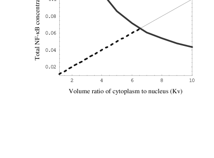
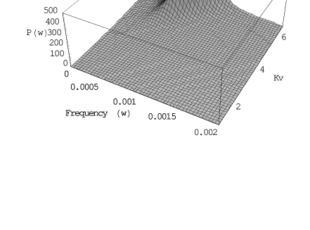
Figure 3: Phase diagram and power spectra for the case of I$\kappa$B knocked-out mutant. (A) shows the phase diagram of NF-$\kappa$B oscillations. (B) demonstrates the power spectra of nuclear NF-$\kappa$B along the diagonal direction in (A) (dashed line).

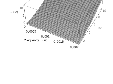
Figure 4: Power spectra for the case of A20 knocked-out mutant. The phase diagram is not present because it contains a dynamically stable region. (A) shows the power spectra along the diagonal direction from Kv=1 to Kv=10.

In Fig. 3, even though I$\kappa$B negative feedback loop is absent, the overall qualitative dynamic features are invariant: the similar deterministic bifurcation curve as well as the similar power spectra. The only difference is that the deterministically dynamical instability domain is reduced slightly. But, the NIO of the NF-$\kappa$B is still observed just outside of the dynamical instability domain. But, in Fig. 4, when A20 negative feedack loop is knocked out, the entire phase plane is deterministically stable in the biologically feasible parameter domain. The inclusion of noise doesn’t induce NIO of the NF-$\kappa$B.

8 Conclusion

We investigate the underlying mechanism of the biological oscillations of the NF-$\kappa$B signaling system by using a stochastic reduced order model and a small noise approximation. This analysis strongly hints that the noise-induced oscillation may be the source of the biological oscillations of NF-$\kappa$B in single cells. First, the oscillations of NF-$\kappa$B are driven by two negative feedback loops in deterministic dynamic system. Second, the stochastic fluctuations in the system induce the NF-$\kappa$B oscillations at the point where the deterministic system generates a stable dynamics because the noise can kick off the system away from its stable fixed point and the sytem takes a long excursive phase trajectory due to the closeby dynamic instability. The NIO of NF-$\kappa$B is robut against the deletion of I$\kappa$B negative feedback loop, but is not when A20 negative feedback loop is deleted. Thus, A20 may be essentially required for NF-$\kappa$B oscillations in single cells.

Appendix A Appendix: Fast transition approximation between NF-$\kappa$B protein and DNA for transcription of I$\kappa$B and A20

The five component model described in the transitions $T_{8}$ and $T_{10}$ in Eq. (1) oversimplifies the very stochastic nature of transcription and translation, starting from $Y$ copy number of nuclear NF-$\kappa$B and ending with creation of a protein C or D, into a linear model. The mathematical description and its analysis of a DNA-protein interaction becomes far more complicated when the exclusiveness of the DNA operator site is taken into account, i.e, once a DNA operator site for a gene C is occupied, the remaining proteins can access no longer to the same operator site unless it is unoccupied. Here we attempt to incorporate the probabilitic operator transition into the model in Eq. (1), by modifying especially two transitions, $T_{8}$ and $T_{10}$.

We briefly describe a probabilistic model of DNA-protein interactions between nuclear NF-$\kappa$B and two I$\kappa$B and A20 promoters. A Fig. 5 shows a transition between four different DNA operator states, i.e., four different combinations each of which consists of a state of I$\kappa$B promoter and one of A20 promoter. $P^{r,s}_{t}$ stands for a joint probability of having a $r$ state of I$\kappa$B promoter and a $s$ state of A20 promoter and $r$ and $s$ can take either 0 (unbounded) or 1 (NF-$\kappa$B-bound). We take a simplest assumption: (1) a transition can change only the state of a single promoter. (2) The change of the state of a promoter isn’t influenced by and doesn’t affect the state of the other promoter. The transition from bounded I$\kappa$B promoter state to I$\kappa$B promoter-free state is denoted by $q_{0}$ and transition from I$\kappa$B promoter-free to I$\kappa$B promoter-bound state is by $q_{1}$ (likewise, $k_{0}$ and $k_{1}$ for A20). By stating that A20 mRNA synthesis rate is $\alpha_{s}$ and I$\kappa$B mRNA synthesis rate is $\beta_{r}$ regardless of the A20 promoter state, we can write a time evolution of a joint probability $P^{r,s}_{t}(C;D)$ of having the $C$ and $D$ copies of I$\kappa$B and A20 mRNA:

$$\frac{dP^{r,s}_{t}(C,D)}{dt} = \alpha_{s}(P^{r,s}_{t}(C;D-1)-P^{r,s}_{t}(C;D))+\beta_{r}(P^{r,s}_{t}(C-1;D)$$

$$- P^{r,s}_{t}(C;D))+q_{r}P^{\hat{r},s}_{t}-q_{\hat{r}}P^{r,s}_{t}+k_{s}P^{r,\hat{s}}_{t}-k_{\hat{s}}P^{r,s}_{t}$$

where $\hat{r}=(r+1)$ mod 2 and $\hat{s}=(s+1)$ mod 2. There are four coupled equation like the above for the different combinations of $(r,s)$, e.g., (0,0), (0,1), (1,0), (1,1).

We define four new variables (marginal probabilities) among which only one variable will survive and the others will go extinct in the limit of fast transition (which parameter?).

$$W_{t}(C;D) \equiv \sum_{s,r}P^{r,s}(C;D)$$ (12)

$$X_{t}(C;D) \equiv k_{1}(P^{0,0}+P^{1,0})-k_{0}(P^{0,1}+P^{1,1})$$

$$Y_{t}(C;D) \equiv q_{1}(P^{0,0}+P^{0,1})-q_{0}(P^{1,0}+P^{1,1})$$

$$Z_{t}(C;D) \equiv (k_{1}+q_{1})P^{0,0}+(k_{0}+q_{0})P^{1,1}-(k_{o}+q_{1})P^{0,1}-(k_{1}+q_{0})P^{1,0}$$

Here W, X, Y, and Z measures are four unique combinations which can be made of two groups, each group being composed of a choice of two original states. X, Y, and Z describes the inflow and the outflow between those two groups denoted by the respective transition rates and will be nullified In the long time limit because the steady state flow between two chosen groups should be balanced. After the substitution of $P^{r,s}$ with new variables $W,X,Y$, and Z, we obtain time evolution equation of a new variable $W_{t}(C;D)$ as follows:

$$\frac{dW_{t}(C;D)}{dt} = \frac{q_{0}\beta_{0}+q_{1}\beta_{1}}{q_{0}+q_{1}}(W_{t}(C-1;D)-W_{t}(C;D))+\frac{k_{0}\alpha_{0}+k_{1}\alpha_{1}}{k_{0}+k_{1}}(W_{t}(C;D-1)-W_{t}(C;D))$$

$$+ \frac{\alpha_{0}-\alpha_{1}}{k_{0}+k_{1}}(X_{t}(C;D-1)-X_{t}(C;D))+\frac{\beta_{0}-\beta_{1}}{q_{0}+q_{1}}(Y_{t}(C-1;D)-Y_{t}(C;D))$$

$$= \frac{q_{0}\beta_{0}+q_{1}\beta_{1}}{q_{0}+q_{1}}(W_{t}(C-1;D)-W_{t}(C;D))+\frac{k_{0}\alpha_{0}+k_{1}\alpha_{1}}{k_{0}+k_{1}}(W_{t}(C;D-1)-W_{t}(C;D))$$

$$+ \frac{k_{0}k_{1}(\alpha_{0}-\alpha_{1})^{2}}{(k_{0}+k_{1})^{3}}(W_{t}(C;D)-2W_{t}(C;D-1)+W_{t}(C;D-2))$$

$$+ \frac{q_{0}q_{1}(\beta_{0}-\beta_{1})^{2}}{(q_{0}+q_{1})^{3}}(W_{t}(C;D)-2W_{t}(C-1;D)+W_{t}(C-2;D))$$

The time-evolution equations of the other three variables, X, Y, and Z, rapidly approaches their respective quasi-steady states in the limit of fast transition (we can show dX/dt =-$\gamma$X+… in the limit of large $\gamma$ value.). The expressions in the last two lines are obtained from setting the time evolution equations of X and Y to zero and assuming the second derivatives of X, Y, and Z with respect to C and D (See my notes for details).

Then, we will perform a small noise approximation of a master equation describing fast operator transition presented in Eq. (LABEL:master_equation_fast_operator). We define three new transitions which decribe the association and the dissociation of the nuclear NF-$\kappa$B proteins with two distinct DNA promotors for gene I$\kappa$B and A20 and the DNA-state dependent protein synthesis.

$$\delta_{1} = \delta^{0}_{1}\Omega_{N}(\frac{Y_{t}}{\Omega_{N}})[DNA]=\delta^{0}_{1}Y_{t}$$ (14)

$$\delta_{0} = \delta^{0}_{0}\Omega_{N}[DNA]=\delta^{0}_{0}\Omega_{N}$$

$$\gamma_{1/0} = \gamma^{0}_{1/0}\Omega_{C}(\frac{RPII}{\Omega_{N}})[DNA]=\gamma^{0}_{1/0}\Omega_{C}$$

where $\delta$ can be either $q$ for I$\kappa$B promotor or $k$ for A20 promotor and $\gamma$ can take either $\alpha$ for I$\kappa$B protein synthesis or $\beta$ for A20 protein synthesis whose transitions are depicted in Fig. 5. We separate the protein-DNA interactions from the actual transcription events which involve RNA polymerase II recruitement and transcriptional elongation, and mRNA synthesis, and protein production in Ribosome. Again, we lump two mRNA and protein syntheses into an effective event represented by $\gamma$ reaction for reduction of model dimension and simplicity of mathematical analysis. Here we assume a binary reaction between DNA promotor site and NF-$\kappa$B protein for $\delta_{1}$ and between RNA polymerase and DNA operator site for $\gamma$. Also, we assume a constant concentration of DNA promotor in nucleus and that of RNA polymerase in nucleus and absorb each into the corresponding reaction rate.

After substituting $Y_{t}$ with van Kampen’s Ansatz and taking a continuum approximation of a step operator, we can rewrite the Eq. (LABEL:master_equation_fast_operator) as follows:

$$\frac{W_{t}(C;D)}{dt} = \frac{\partial\omega_{t}(\xi_{C};\xi_{D})}{\partial t}-\sum_{C,D}\Omega^{1/2}_{C}\frac{d\alpha}{dt}\frac{\partial\omega_{t}(\xi_{C};\xi_{D})}{\partial\xi_{\alpha}}$$

$$= -\Omega^{1/2}_{C}(A^{D}\frac{\partial}{\partial\xi_{D}}+A^{C}\frac{\partial}{\partial\xi_{C}})\omega_{t}(\xi_{C};\xi_{D})$$

$$+ \Omega^{0}_{C}(\frac{\partial^{2}B^{D}}{\partial\xi^{2}_{D}}+\frac{\partial^{2}B^{C}}{\partial\xi^{2}_{C}}-\sqrt{K_{v}}\frac{\partial C^{D}}{\partial\xi_{D}}-\sqrt{K_{v}}\frac{\partial C^{C}}{\partial\xi_{C}})\omega_{t}(\xi_{C};\xi_{D})+O(\Omega^{-1/2})$$

where

$$A^{D} = \frac{k^{0}_{0}\alpha^{0}_{0}+k^{0}_{1}\alpha^{0}_{1}y}{k^{0}_{0}+k^{0}_{1}y}$$ (16)

$$B^{D} = A^{D}+\frac{k^{0}_{0}k^{0}_{1}(\alpha^{0}_{0}-\alpha^{0}_{1})^{2}yK_{v}}{(k^{0}_{0}+k^{0}_{1}y)^{3}}$$

$$C^{D} = \frac{k^{0}_{1}\xi_{Y}}{k^{0}_{0}+k^{0}_{1}y}(\alpha^{0}_{1}-\frac{k^{0}_{0}\alpha^{0}_{0}+k^{0}_{1}\alpha^{0}_{1}y}{k^{0}_{0}+k^{0}_{1}y})$$

$$A^{C} = \frac{q^{0}_{0}\beta^{0}_{0}+q^{0}_{1}\beta^{0}_{1}y}{q^{0}_{0}+q^{0}_{1}y}$$

$$B^{C} = A^{C}+\frac{q^{0}_{0}q^{0}_{1}(\beta^{0}_{0}-\beta^{0}_{1})^{2}yK_{v}}{(q^{0}_{0}+q^{0}_{1}y)^{3}}$$

$$C^{C} = \frac{q^{0}_{1}\xi_{Y}}{q^{0}_{0}+q^{0}_{1}y}(\beta^{0}_{1}-\frac{q^{0}_{0}\beta^{0}_{0}+q^{0}_{1}\beta^{0}_{1}y}{q^{0}_{0}+q^{0}_{1}y})$$

in the derivation, we use a taylor expansion of the transition rate in the limit of a large volume $\Omega_{C}$, e.g., $1/(1+\frac{k^{0}_{1}\xi_{Y}\Omega^{-1/2}_{C}}{k^{0}_{0}+k^{0}_{1}y})^{N}\sim 1-N\frac{k^{0}_{1}\xi_{Y}\Omega^{-1/2}_{C}}{k^{0}_{0}+k^{0}_{1}y}$.

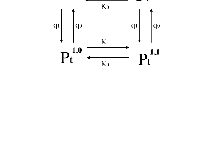
Figure 5: Transition between four states consisting of I$\kappa$B and A20 promoters. $P^{r,s}_{t}$ stands for the probability having ”r” state of the I$\kappa$B promoter and ”s” state of the A20 promoter. The transition between two states is denoted by a transition rate, either $q$ or $K$.

References

- [1] Murray JD (1980) Mathematical Biology, Springer-Verlag, New York, 1980.
- [2] Lahav G, Rosenfeld N, Sigal A, Geva-Zatorsky N, Levine AJ, Elowitz MB, Alon U (2004) Dynamics of the p53-Mdm2 feedback loop in individual cells. Nat. Genet. 36: 147-150.
- [3] Nelson DE, Ihekwaba AEC, Elliott M, Johnson JR, Gibney CA, Foreman BE, Nelson G, See V, Horton CA, Spiller DG, Edwards SW, McDowell HP, Unitt JF, Sullivan E, Grimley R, Benson N, Broomhead D, Kell DB, White MRH (2004) Oscillations in NF-B signaling control the dynamics of gene expression. Science 306: 704-708.
- [4] Steuer, R. (2004) Effects of stochasticity in models of the cell cycle: from quantized cycle times to noise-induced oscillations. J. Thoer. Biol. 228: 293-301.
- [5] Pikovsky, A. S., and J. Kurths. 1997. Coherence resonance in a noise-driven excitable system. Phys. Rev. Lett. 78: 775-778.
- [6] Neiman, A, P. I. Saparin, and L. Stone. 1997. Coherence resonance at noisy precursors of bifurcations in nonlinear dynamical systems. Phys. Rev. E. 56: 270-273.
- [7] Gammaitoni, L., P. Hanggi, P. jung, and F. Marchesoni. 1998. Stochastic resonance. Rev. Mod. Phys. 70: 223-287.
- [8] Benzi, R., G. Parisi, A. Sutera, and A. Vulpiani. 1982. Stochastic resonance in climate change. Tellus 34:10-16.
- [9] Wiesendfeld, K. (1985) Noisy precursors of nonlinear instabilities. J. Stat. Phys. 38: 1071-1096.
- [10] Gang, H., T. Ditzinger, C. Z. Ning, and H. Haken (1993) Stochastic resonance without external periodic force. Phys. Rev. Lett. 71: 807-810.
- [11] McKane, A. J., J. D. Nagy, T. J. Newman, and M. O. Stefanini (2007). Amplified biochemical oscillations in cellular systems. J. Stat. Phys. 128:165-191.
- [12] Joo J, Plimpton S, Faulon JL, 2009. Noise-induced oscillatory shuttling of NF-B in a two compartment IKK-NF-B-IB-A20 signaling module. LANL preprint archive arXiv:1010.0888.
- [13] Joo J, Plimpton S, Martin S, Swiler L, Slepoy A, Faulon JL, (2007). Sensitivity analysis of computational model of the IKK-NF-kappaB-IkappaBalpha-A20 signal transduction network, Annals of the NY Academy of Sciences, 1115:221-239.
- [14] Van Kampen, NG (2001) Stochastic Processes in Physics and Chemistry, North-Holland, New York.