Nucleon-Nucleon interaction, charge symmetry breaking and renormalization

Abstract

We study the interplay between charge symmetry breaking and renormalization in the $NN$ system for $s-$waves. We find a set of universality relations which disentangle explicitly the known long distance dynamics from low energy parameters and extend them to the Coulomb case. We analyze within such an approach the One-Boson-Exchange potential and the theoretical conditions which allow to relate the proton-neutron, proton-proton and neutron-neutron scattering observables without the introduction of extra new parameters and providing good phenomenological success.

I Introduction

The understanding of Charge Dependence of strong interactions has been a crucial issue in Nuclear Physics (for reviews see e.g. Wilkinson (1969); Miller et al. (1990); Machleidt and Slaus (2001); Miller et al. (2006)). In fact, the simplest place where this issue can be studied is the nucleon-nucleon interaction. As it is well known, isospin invariance is not an exact symmetry of strong interactions. As a consequence nuclear forces have a small but net charge-dependent component. By definition, charge independence means invariance under any rotation in isospin space. A violation of this symmetry is referred to as charge dependence or charge independence breaking (CIB) and it means in particular that, in the isospin $T=1$ state, the proton-proton ($T_{3}=+1$), neutron-proton ($T_{3}=0$), or neutron-neutron ($T_{3}=-1$) strong interactions are different. A particular case, known as charge symmetry breaking (CSB), only considers the difference between proton-proton ($pp$) and neutron-neutron ($nn$) interactions. Further corrections are expected when, in addition, Coulomb forces are added to the proton-proton system ($pp(c)$).

But, what is the scale of charge symmetry breaking?. Actually, the effects are important in the s-wave channel where an unnaturally large scattering length, due to a virtual state  in that partial wave, triggers a high short distance sensitivity. This, of course amplifies effects related to variations in the short distance parameters precisely in the region where the interaction and hence the charge symmetry breaking effects may be less reliable. The current understanding is that CIB, and in particular CSB, are due to a mass difference between the up and down quarks and electromagnetic interactions. On the hadronic level and in a One-Boson-Exchange (OBE) based picture (such as e.g. Machleidt et al. (1987)), major causes of CIB and CSB are effects explicitly related to

• Different proton and neutron masses.

• Electromagnetic effects (mainly Coulomb interaction).

• Mass splitting of isovector mesons $\pi$ and $\rho$ and different coupling constants.

• Mass splitting between different $\Delta$-isobar charge states.

• Unknown short distance effects which are usually described by models.

Traditionally it is believed that the difference between the charge and neutral pion mass in the One-Pion-Exchange (OPE) potential accounts for a big part of CIB while the difference between the masses of neutron and proton represents the most basic cause for CSB. Pion mass differences were shown to account for a $80\%$ of the $nn$-$pp$ scattering length difference Cheung and Machleidt (1986). The nucleon mass splitting also generates a difference in the kinetic energies. Some recent OBE models only consider the differences coming from nucleon mass splitting and kinematical effects Stoks et al. (1994); Wiringa et al. (1995). However, these effects can only explain about a $15\%$ of the empirical CSB. As a consequence some models leave CSB unexplained Stoks et al. (1994) while others simply introduce a term ad hoc to explain the remaining contribution Wiringa et al. (1995). In Ref. Li and Machleidt (1998a) $2\pi$-exchange contributions, $\pi\rho$ diagrams and other multi-meson exchanges including the $\Delta$-isobar as intermediate states were considered to explain the empirical CSB value accurately. In Ref. Li and Machleidt (1998b) $2\pi$-exchange contributions with $\Delta$ were found to be noticeable to explain the empirical CIB value being $3\pi$- and $4\pi$-exchanges negligible. The difficulties arising in multi-meson exchange diagrams, in particular the energy dependence that they create, were avoided in the Bonn potential Machleidt et al. (1987) by introducing two effective scalar-isoscalar $\sigma$-mesons simulating $2\pi+\pi\rho$ exchanges. In the highly successful CD-Bonn potential Machleidt (2001) CSB was included at the simplest one-boson-exchange diagrams with the same philosophy as its predecessor Machleidt et al. (1987).

Many authors have also proposed the $\rho-\omega$ mixing as a key ingredient to understand CSB Machleidt and Muther (2001); Biswas et al. (2008). In Ref. Machleidt and Muther (2001) the $\rho-\omega$ mixing is identified as the major source of CSB while proton and nucleon mass differences are identified to produce a minor effect. It should be noted that such a calculation is hampered by the fact that the $g_{\omega NN}$ coupling constant occurring in the CS part is about $40\%$ larger than expected from $SU(3)$ ($g_{\omega NN}=3g_{\rho NN}\sim 9$) and also from the actual value taken for the CSB potential. Fixed-s Dispersion relations Hamilton and Oades (1984) yielded $g_{\omega NN}=5.7\pm 2.0$ and Vector Meson Dominance $\omega\to e^{+}e^{-}$ decays prefer $g_{\omega NN}\sim 10$. The $\eta-\pi^{0}$ has been shown to be of some relevance as well Piekarewicz (1993).

The high sensitivity has been a major motivation to pursue experimental determinations of the neutron-neutron scattering length by indirect methods (for a review see e.g. Ref. Howell (2008) and references therein). A recent measurement of the nn scattering length using the pi-d capture reaction, yields (see also Gardestig (2009) for a review ) $a_{nn}=-18.69(4)\,{\rm fm}$ when corrected for magnetic interactions. The recent CSB analysis of the reaction $dd\to\pi^{0}\alpha$ Fonseca et al. (2009) uses also the large $g_{\omega NN}$ constant.

The purpose of the present work is to approach the problem from a renormalization point of view. While we consider long distance physics to be known and describable by non-relativistic potentials we use a physical low energy parameter such as the scattering length to encode the unknown short distance physics. For the Charge Independent case it was shown how a natural $SU(3)$ value of $g_{\omega NN}$ could be confortably taken if a certain renormalization condition was imposed Calle Cordon and Ruiz Arriola (2008); Calle Cordon and Ruiz Arriola (2010). As we will discuss in much detail this poses a problem of finiteness in physical observables when connecting different channels such as $np$, $nn$ and $pp$ (strong or Coulomb). We propose a short distance renormalization condition featuring charge independence which guarantees finiteness although an ambiguity arises. However, a natural choice of the renormalization condition works quite well when compared to measured or recommended values. While the traditional point of view outlined above tried to compute the scattering lengths, the Effective Field Theory (EFT) approach assumes that these scattering lengths are completely unrelated Kong and Ravndal (1999, 2000); Walzl et al. (2001); Gegelia (2004); Epelbaum and Meissner (2005); Ando et al. (2007). We pursue here the possible connection between them from a new perspective which actually is in-between, combining both points of view. We assume one scattering length to be known and exploit the concept of short distance insensitivity to determine all other scattering lengths and phase shifts from the requirement of finiteness of the scattering amplitude.

The paper is organized as follows. In Section II we motivate the use of renormalization without assuming previous knowledge from the reader as a useful preparatory material for further developments. In Section III we extend the results to the interesting case of long range Coulomb interactions as they appear in $pp$ scattering. CSB interactions are studied in all separate $np$,$nn$,$pp$ and $pp(c)$ cases in Section IV where insightfull universal relations are found out. In Section V we propose a short distance connection where all the channels are correlated from the requirement of finiteness. A further interesting application has to do with the determination in Appendix A of the Gamow-Teller matrix element needed in the pp fusion process from the np scattering length. Finally, in Section VI we come to the conclusions.

II The standard vs. the renormalization approach

II.1 The OBE potential

In this section we briefly review the main ideas behind renormalization in coordinate space for the OBE potentials (for a more detailed account see e.g. Ref. Calle Cordon and Ruiz Arriola (2010)) since they are focal in what follows. To provide a comprehensive perspective we compare it with the more traditional viewpoint of regulating the singular meson-exchange potentials by means of the introduction of short-distance form factors. The crucial distinction lies in the sensitivity to short-distance details: from the renormalization point of view we expect complete insensitivity to these details. On the contrary, a regularization procedure only guarantees the finiteness of the results. For definiteness, let us analyze as an illustrative example the phenomenologically successful ${}^{1}S_{0}$ one boson exchange (OBE) potential Machleidt (2001); Machleidt et al. (1987)

$$V(r) = -\frac{g_{\pi NN}^{2}m_{\pi}^{2}}{16\pi M_{N}^{2}}\frac{e^{-m_{\pi}r}}{r}-\frac{g_{\sigma NN}^{2}}{4\pi}\frac{e^{-m_{\sigma}r}}{r}$$ (1)

$$+ \frac{g_{\omega NN}^{2}}{4\pi}\frac{e^{-m_{\omega}r}}{r}-\frac{f_{\rho NN}^{2}m_{\rho}^{2}}{8\pi M_{N}^{2}}\frac{e^{-m_{\rho}r}}{r}\,,$$

where $g_{\sigma NN}$ is a scalar type coupling, $g_{\pi NN}$ a pseudo-scalar coupling, $g_{\omega NN}$ is a vector coupling and $f_{\rho NN}$ is a tensor derivative coupling (see Machleidt et al. (1987) for notation). We neglect for simplicity nucleon mass effects and a tiny $\eta$ contribution. We take $m_{\pi}=138{\rm MeV}$, $M_{N}=939{\rm MeV}$, $m_{\rho}=770{\rm MeV}$, $m_{\omega}=783{\rm MeV}$ and $g_{\pi NN}=13.1$ which seem firmly established. The OBE potential, Eq. (1) corresponds to a long distance expansion of the potential. On the other hand, NN scattering in the elastic region below pion production threshold involves CM momenta $p<p_{\rm max}=400{\rm MeV}$. Given the fact that $1/m_{\omega}=0.25\,{\rm fm}\ll 1/p_{\rm max}=0.5\,{\rm fm}$ we expect heavier mesons to be irrelevant, and $\rho$ and $\omega$ themselves to be of marginal important. This naive expectation is, however, not fulfilled in the traditional approach Machleidt (2001); Machleidt et al. (1987).

In the following we will make the approximation $m_{\rho}=m_{\omega}$, specially when making fits of the coupling parameters to the ${}^{1}S_{0}$ phases. Under the previous approximation is convenient to define

$$g_{\omega NN}^{*}=\sqrt{g_{\omega NN}^{2}-\frac{f_{\rho NN}^{2}m_{\rho}^{2}}{2M_{N}^{2}}}\,,$$ (2)

in such a way that the combined $\omega-\rho$ potential reads

$$\frac{g_{\omega NN}^{2}}{4\pi}\frac{e^{-m_{\omega}r}}{r}-\frac{f_{\rho NN}^{2}m_{\rho}^{2}}{8\pi M_{N}^{2}}\frac{e^{-m_{\rho}r}}{r}\simeq\frac{{g_{\omega NN}^{*}}^{2}}{4\pi}\frac{e^{-m_{\omega}r}}{r}\,.$$ (3)

The previous simplification is useful since it avoids correlations between $g_{\omega NN}$ and $f_{\rho NN}$ in the ${}^{1}S_{0}$ channel. For SU(3) values of $g_{\omega NN}\sim 9$ or VMD $\omega\to e^{+}e^{-}$ e.m. decays $g_{\omega NN}\sim 10.5$ and typical $\rho$-tensor values $f_{\rho NN}\sim 14-18$ one has $g_{\omega NN}^{*}\sim 0-7$.

II.2 Regular solution

In the traditional approach Machleidt et al. (1987); Machleidt (2001) the problem is essentially handled by solving the reduced Schrödinger equation, which for the $s-$wave case reads

$$-u_{k}^{\prime\prime}(r)+M_{N}\,V(r)u_{k}(r)=k^{2}u_{k}(r)\,,$$ (4)

with $k=\sqrt{M_{N}E}$ the center-of-mass momentum, $M_{N}$ the nucleon mass, and $V(r)$ the boson-exchange potential of Eq. (1). The Schrödinger equation is a second order differential equation and it has two linearly independent solutions. The physical solution is usually determined by the regularity condition at the origin, i.e.

$$u_{k}(0)=0\,.$$ (5)

This boundary condition for the Schrödinger equation implicitly assumes that we are taking the potential seriously all the way down to the origin .

The asymptotic behaviour of the reduced wave function for $r\gg 1/m_{\pi}$ is given by

$$u_{k}(r)\to\frac{\sin(kr+\delta_{0}(k))}{\sin\delta_{0}(k)}\,,$$ (6)

where $\delta_{0}(k)$ is the s-wave phase shift. For the potential described by Eq. (1), the phase shift is an analytic function of $k$ with branch cuts located at $k=\pm im_{\pi}/2$, $\pm im_{\sigma}/2$, etc. This means in particular that for momenta below the first branch cut, $|k|\leq m_{\pi}/2$, we can expand the phase shift by means of the effective range expansion Bethe (1949)

$$k\,\cot\delta_{0}(k)=-\frac{1}{\alpha_{0}}+\frac{1}{2}r_{0}k^{2}+v_{2}k^{4}+\dots\,,$$ (7)

where $\alpha_{0}$ is the scattering length, $r_{0}$ the effective range and $v_{2}$ the shape parameter.

The effective range parameters can be related with the expansion of the wave function in terms of $k^{2}$, i.e.

$$u_{k}(r)=u_{0}(r)+k^{2}u_{2}(r)+\dots\,,$$ (8)

where $u_{0}$ and $u_{2}$ obey the following equations

$$-u_{0}^{\prime\prime}(r)+M_{N}\,V(r)u_{0}(r) = 0\,,$$ (9)

$$-u_{2}^{\prime\prime}(r)+M_{N}\,V(r)u_{2}(r) = u_{0}(r)\,,$$ (10)

subjected to regular boundary conditions, $u_{0}(0)=u_{2}(0)=0$, and asymptotically normalized to

$$u_{0}(r) \to 1-r/\alpha_{0}\,,$$ (11)

$$u_{2}(r) \to \left(r^{3}-3\alpha_{0}r^{2}+3\alpha_{0}r_{0}r\right)/(6\alpha_{0})\,,$$ (12)

for $r\gg 1/m_{\pi}$. With this normalization, the effective range $r_{0}$ is computed from the standard formula

$$r_{0} = 2\int_{0}^{\infty}dr\left[\left(1-r/\alpha_{0}\right)^{2}-u_{0}(r)^{2}\right]\,.$$ (13)

In the traditional approach Machleidt et al. (1987); Machleidt (2001) everything is obtained from the potential, which is assumed to be valid for $0\leq r<\infty$. In practice, strong form factors are included mimicking the finite nucleon size and reducing the short distance repulsion of the potential, but the regular boundary condition is always kept. One of the problems with this point of view has to do with the fact that the ${}^{1}S_{0}$ scattering length is unnaturally large $\alpha_{0}=-23.74(2){\rm fm}$, while the effective range is natural, $r_{0}=2.77(4){\rm fm}$ (approximately twice the pion Compton wave length, $\sim 2/m_{\pi}$). This has dramatic consequences regarding the short distance sensitivity, as we will show below.

BC	$r_{c}({\rm fm})$	$m_{\sigma}({\rm MeV})$	$g_{\sigma NN}$	$g_{\omega NN}^{*}$	$\chi^{2}/DOF$	$\alpha_{0}({\rm fm})$	$r_{0}({\rm fm})$
Regular solution-I	0	498.2(7)	9.488(11)	7.94(2)	0.480	-23.737	2.678
Regular solution-II	0	550.72(4)	13.87(13)	20.10 (24)	0.674	-23.738	2.679
Renormalizing	0	490(17)	8.7(6)	0(5)	0.289	input	2.672

Table 1: Fits to the ${}^{1}S_{0}$ phase shift of the Nijmegen group Stoks et al. (1994) using the OBE potential with a charge dependent OPE part. We take $m_{\pi^{0}}=134.97\,{\rm MeV}$, $m_{\pi^{+}}=139.57\,{\rm MeV}$, $g_{A}=1.29$ and $f_{\pi}=92.4\,{\rm MeV}$ de Swart et al. (1997). We neglect the CSB coming from the $\rho$-meson and take $m_{\rho}=m_{\omega}=770\,{\rm MeV}$ fitting $m_{\sigma}$, $g_{\sigma NN}$ and $g_{\omega NN}^{*}$. We use the value $\alpha_{np}=-23.74\,{\rm MeV}$ as an input when renormalizing.

A fit to the $np$ averaged data of Ref. Stoks et al. (1994) in the ${}^{1}S_{0}$ channel yields two possible solutions, see Table 1. Thus, we have two good incompatible fits. A remarkable aspect is the fact that the vector meson coupling constant is accurately well determined. Actually, if we assume that we have fitted the potential, Eq. (1), to reproduce $\alpha_{0}$, a tiny change in the potential $V\to V+\Delta V$ has a dramatic effect on $\alpha_{0}$, since one obtains

$$\Delta\alpha_{0}=\alpha_{0}^{2}M_{N}\int_{0}^{\infty}\Delta V(r)u_{0}(r)^{2}dr\,,$$ (14)

a quadratic effect in the large $\alpha_{0}$. As a result, potential parameters must be fine tuned, as can be deduced from the previous fits. Thus, despite the undeniable success in fitting the data, this sensitivity to short distances looks counterintuitive.

However it is worth mentioning that the different scenarios correspond to selecting a potential possessing spurious bound states or not. The spurious bound state problem has been discussed in Ref. Calle Cordon and Ruiz Arriola (2010) at length; the number of inner zeroes of the zero energy wave function provides the number of bound states. For illustration we represent the zero energy wave in Fig 1. In the regular case, the OBE potential with a big $g_{\omega NN}^{*}$ is free of bound states. However if a small $g_{\omega NN}^{*}$ is chosen, then one has to deal with a bound state which does not exist and it is hence spurious.

Figure 1: Zero energy wave function for the singlet $np$ ${}^{1}S_{0}$ channel as a function of distance (in fm) and for the different scenarios with large and small $\omega-$couplings. This wave function goes asymptotically to $u_{0}(r)\to 1-r/\alpha_{0}$ with $\alpha_{0}=-23.74{\rm fm}$ the scattering length in this channel. The zero at about $r=0.5{\rm fm}$ signals the existence of a spurious bound state.

II.3 Irregular solutions

The previous results are in conflict with the intuitive expectation of insensitivity of low energy physical observables with respect to the specific details of the potential in the short distance region. Otherwise, where should one stop ?. This is the basis of the renormalization viewpoint. The way to proceed is to impose renormalization conditions which eliminate the short range sensitivity at the expense of treating low energy parameters as independent variables from the potential. An example of a renormalization condition (RC) is to fix the scattering length, with the consequence of avoiding the fine tuning problem summarized by Eq. (14). In other words, we trade the explicit dependence of the results on the short range parameters of the potential for low energy observables. The values of the later are usually well-known by other means.

In principle there are several ways in which one can impose renormalization conditions, one popular example being counterterms. They correspond to the coupling constants of a short distance contact potential which is expanded in terms of $\delta$ functions and its derivatives

$$V_{C}(\vec{x})=C_{0}\,\delta(\vec{x})+C_{2}\,\{\nabla^{2},\delta(\vec{x})\}+\dots\,,$$ (15)

where the dots represent terms involving higher derivatives of the $\delta$ function. This potential is added to the usual finite range potential $V$, and then the corresponding Schrödinger equation for $V_{C}+V$ is solved. The resulting potential is strongly singular and needs to be regularized by introducing a cut-off $r_{c}$, a length scale which is used to smear the $\delta$ functions. The different coupling constants $C_{0}(r_{c})$, $C_{2}(r_{c})$, etc, are set to reproduce the desired low-energy observables. A nice presentation of the previous method is given in Ref. Lepage (1997). The disadvantage is that the procedure of using a potential to renormalize quickly runs into problems when one tries to decrease the size of the cut-off. For example, it may be impossible to reproduce certain physical observables, specifically the effective range, if the short distance cut-off is too small Phillips and Cohen (1997), unless one accepts complex values for the counterterms $C_{0}(r_{c})$ and $C_{2}(r_{c})$ which violate either causality or off-shell unitarity (see Ref. Entem et al. (2008) for a detailed discussion). Related positivity conditions are discussed in Ref. Calle Cordon and Ruiz Arriola (2010).

Here we use a more indirect method to renormalize which is able to avoid some of the previously mentioned complications. The idea is to substitute the regularity condition of the Schrödinger equation, $u_{k}(0)=0$, by an arbitrary boundary condition at the origin

$$L_{k}(0)=\frac{u_{k}^{\prime}(0)}{u_{k}(0)}\,,$$ (16)

where we have used the log-derivative of the wave function, instead of an independent condition for $u_{k}(0)$ and $u_{k}^{\prime}(0)$, as that will only affect the precise normalization of the wave function, which can be later determined by other means. The regularity condition $u_{k}(0)=0$ corresponds to taking the limit $L_{k}(0)\to\infty$ (as $u_{k}^{\prime}(0)$ is a constant), but by changing the precise value and energy dependence $L_{k}(0)$, the values of low energy observables can be fixed.

The previous procedure would in principle involve a fitting procedure, which can be avoided by taking into account the expansion in powers of $k$ of the wave function, Eq. (8). For example, if we want to fix the scattering length, we will solve the corresponding equation for the zero-energy wave function $u_{0}(r)$, with the asymptotic ($r\to\infty$) boundary condition of reproducing the scattering length

$$-u_{0}^{\prime\prime}(r)+M_{N}\,V(r)u_{0}(r) = 0\,,$$ (17)

$$u_{0}(r) \to 1-\frac{r}{\alpha_{0}},$$ (18)

but, instead of solving the previous equation from $r=0$ to $r\to\infty$, we solve it downwards from infinity to the origin. Then, we assume that $u_{2}(r)$, $u_{4}(r)$, etc, are subjected to regular boundary conditions at the origin, $u_{2}(0)=u_{4}(0)=0$ and $u_{2}^{\prime}(0)=u_{4}^{\prime}(0)=0$, which means to take

$$L_{k}(0)=\frac{u_{0}^{\prime}(0)}{u_{0}(0)}\,.$$ (19)

By so doing we achieve some insensitivity at short distances, as we will show later . Fixing more scattering parameters is straightforward: one solves downwards the corresponding equations for $u_{0}(r),u_{2}(r),\dots,u_{2n}(r)$ with the asymptotic conditions of reproducing $\alpha_{0},r_{0},\dots,v_{n}$, and assumes trivial boundary conditions for $u_{2n+2}(r)$, $u_{2n+4}(r)$, etc, resulting the following logarithmic boundary condition

$$L_{k}(0)=\frac{u_{0}^{\prime}(0)+k^{2}u_{2}^{\prime}(0)+\dots+k^{2n}u_{2n}^{\prime}(0)}{u_{0}(0)+k^{2}u_{2}(0)+\dots+k^{2n}u_{2n}(0)}\,.$$ (20)

In practical computations it is convenient to introduce a short distance cut-off, $r_{c}$, and then take the limit $r_{c}\to 0$.

A further simplification can be made if we take into account that the OBE potential of Eq. (1) is local and energy independent. This means in particular that different energy states are orthogonal,

$$\int_{0}^{\infty}u_{k}(r)u_{p}(r)dr=0\,,$$ (21)

for $k\neq p$, which requires an energy independent boundary condition at the origin, as a consequence of the next equality

$$\int_{0}^{\infty}u_{k}(r)u_{p}(r)dr=u_{k}^{\prime}u_{p}-u_{p}u_{k}^{\prime}\Big{|}_{0}\,,$$ (22)

which means that the orthogonality condition Eq. (21) can be re-expressed as

$$\frac{u_{k}^{\prime}(0)}{u_{k}(0)}=\frac{u_{p}^{\prime}(0)}{u_{p}(0)}\,,$$ (23)

or, equivalently, $L_{k}(0)=L_{p}(0)$, implying an energy independent boundary condition.

Here we will only consider the case in which orthogonality is preserved. The restriction is that orthogonality implies that we can only fix one scattering parameter, namely the scattering length. Therefore we will integrate downwards the zero energy state, $u_{0}(r)\to 1-{r}/{\alpha_{0}}$, up to the cut-off $r_{c}$. At this point, we can make use of the superposition principle in order to take real advantage of the boundary condition method. For the zero-energy solution, the superposition principle can be used to write the wave function as a linear combination of two independent zero-energy solutions

$$u_{0}(r)=u_{1}(r)-\frac{u_{r}(r)}{\alpha_{0}}\,,$$ (24)

where $u_{1}(r)$ and $u_{r}(r)$ are solutions of the zero-energy Schrödinger equation, Eq. (9), with the asymptotic boundary conditions

$$u_{1}(r) \to 1\,,$$ (25)

$$u_{r}(r) \to r\,,$$ (26)

at large distances. The previous expression for $u_{0}$ as a linear combination, Eq. (24), can be introduced in the integral representation of the effective range $r_{0}$, Eq. (13), yielding the following correlation between $r_{0}$ and $\alpha_{0}$

$$r_{0} = A_{0}+\frac{B_{0}}{\alpha_{0}}+\frac{C_{0}}{\alpha_{0}^{2}}\,,$$ (27)

where $A_{0}$, $B_{0}$ and $C_{0}$ are given by

$$A_{0} = 2\int_{0}^{\infty}dr(1-u_{1}^{2})\,,$$ (28)

$$B_{0} = -4\int_{0}^{\infty}dr(r-u_{1}u_{r})\,,$$ (29)

$$C_{0} = 2\int_{0}^{\infty}dr(r^{2}-u_{r}^{2})\,.$$ (30)

The interesting feature is that the dependence of the effective range with respect to short-range parameters of the potential is greatly diminished.

The short distance sensitivity can be vividly seen in Fig. 2, where the regular (parabola like curve) as well as the renormalized (flat curve) effective range for the OBE potential are shown as a function of $g_{\omega NN}^{*}$. For simplicity only the solution with the small $g_{\omega NN}^{*}$ (Regular solution I) is represented.

Figure 2: Dependence of the effective range with respect to $g_{\omega NN}^{*}$ in the regular case with a small coupling constant and in the renormalized one.

The finite-energy solutions and the phase shifts can be obtained from the orthogonality condition, which implies

$$\lim_{r_{c}\to 0}\frac{u_{k}^{\prime}(r_{c})}{u_{k}(r_{c})}=\lim_{r_{c}\to 0}\frac{u_{0}^{\prime}(r_{c})}{u_{0}(r_{c})}\,,$$ (31)

providing the initial boundary conditions for the finite-energy Schrödinger equation, Eq. (4). We normalize the scattering wave function as follows

$$u_{k}(r)\to\frac{\sin(kr+\delta_{0})}{\sin\delta_{0}}\,.$$ (32)

Again, if we use the superposition principle, $u_{k}$ can be written as

$$u_{k}(r)=k\cot\delta_{0}\,u_{k,s}(r)+u_{k,c}(r)\,,$$ (33)

with $u_{k,c}$ and $u_{k,s}$ solutions of Eq. (4) asymptotically normalized as

$$u_{k,c} \to \cos(kr)\,,$$ (34)

$$u_{k,s} \to \frac{\sin(kr)}{k}\,.$$ (35)

These two wave functions have the property of going to $u_{k,s}\to u_{r}$ and $u_{k,c}\to u_{1}$ for $k\to 0$. Then, the orthogonality constraint Eq. (31) reads

$$\frac{k\cot\delta_{0}u_{k,s}^{\prime}(r_{c})+u^{\prime}_{k,c}(r_{c})}{k\cot\delta_{0}u_{k,s}(r_{c})+u_{k,c}(r_{c})}=\frac{\alpha_{0}\,u_{1}^{\prime}(r_{c})-u_{r}^{\prime}(r_{c})}{\alpha_{0}\,u_{1}(r_{c})-u_{r}(r_{c})}\,,$$ (36)

where we have dropped the $\lim_{r_{c}\to 0}$ for shortening the notation. Note that the dependence of the phase-shift on the scattering length is explicit: $k\cot\delta_{0}$ is a bilinear mapping of $\alpha_{0}$,

$$k\cot\delta_{0}=\frac{\alpha_{0}{\cal A}(k)+{\cal B}(k)}{\alpha_{0}{\cal C}(k)+{\cal D}(k)}\,,$$ (37)

where the functions ${\cal A}$, ${\cal B}$, ${\cal C}$ and ${\cal D}$ are even functions of $k$ which depend solely on the potential and are given by the following formulas

$${\cal A}(k) = \lim_{r_{c}\to 0}\left(u_{1}(r_{c})u^{\prime}_{k,c}(r_{c})-u_{1}^{\prime}(r_{c})u_{k,c}(r_{c})\right)\,,$$

$${\cal B}(k) = \lim_{r_{c}\to 0}\left(u_{k,c}(r_{c})u^{\prime}_{r}(r_{c})-u_{r}(r_{c})u_{k,c}^{\prime}(r_{c})\right)\,,$$

$${\cal C}(k) = \lim_{r_{c}\to 0}\left(u_{1}^{\prime}(r_{c})u_{k,s}(r_{c})-u_{1}(r_{c})u^{\prime}_{k,s}(r_{c})\right)\,,$$

$${\cal D}(k) = \lim_{r_{c}\to 0}\left(u_{r}(r_{c})u^{\prime}_{k,s}(r_{c})-u_{r}^{\prime}(r_{c})u_{k,s}(r_{c})\right)\,.$$

The previous expressions fix the arbitrary normalization of Eq. (37). The obvious conditions ${\cal A}(0)={\cal D}(0)=0$ and ${\cal B}(0)={\cal C}(0)=1$ are satisfied. Expanding the expression for small $k$ one gets that $v_{k}$ is a polynomial in $1/\alpha_{0}$ of degree $k+1$.

Finally, we can use the previous procedure to fit the $np$ averaged data of Ref. Stoks et al. (1994) in the ${}^{1}S_{0}$ channel (once we have fixed the scattering length to its experimental value), yielding the values in table 1. We can see the large uncertainty on the value of $g_{\omega NN}^{*}$, which shows that there is a greater insensitivity to shorter distances after renormalizing. This agrees with the previous remarks on the sensitivity of the effective range on $g_{\omega NN}^{*}$, illustrated in Fig. 2. Let us note further that as discussed in Ref. Calle Cordon and Ruiz Arriola (2010) the renormalization scenario also has also a spurious bound state as in the small $g_{\omega NN}^{*}$ regular solution case (see Fig 1). The current discussion would be modified by the inclusion of form factors which incorporate the finite nucleon size. However, because of the short distance insensitivity form factors turn out to play a marginal role Calle Cordon and Ruiz Arriola (2010) after renormalization .

II.4 Review of the Renormalization Process

The renormalization procedure proposed in this section can be summarized as follows

• For a given scattering length $\alpha_{0}$, integrate in the zero energy wave function $u_{0}(r)$ with Eq. (9) down to the cut-off radius $r_{c}$. This is the renormalization condition.

• Implement self-adjointness at the cut-off radius through the boundary condition

  $$u_{k}^{\prime}(r_{c})u_{0}(r_{c})-u_{0}^{\prime}(r_{c})u_{k}(r_{c})=0\,,$$ (39)

• Integrate out the finite energy wave function $u_{k}(r)$ with Eq. (4) and determine the phase shift $\delta_{0}(p)$ from Eq. (6).

• Remove the cut-off (take the limit $r_{c}\to 0$) to assure model (regulator) independence.

This allows to compute $\delta_{0}$ (and hence $r_{0}$, $v_{2}$ ) from (i) the potential $V(r)$ and (ii) the scattering length $\alpha_{0}$ as independent information. Note that this is equivalent to consider, in addition to the regular solution, the irregular one. In momentum space this can be shown to be equivalent to introduce one counterterm in the cut-off Lippmann-Schwinger equation (see Ref. Entem et al. (2008) for a detailed discussion). Both Eq. (27) and Eq. (37) highlights this de-correlation between the potential and the scattering length. Contrary to common wisdom, but according to our intuitive expectations, no strong short range repulsion is essential. The moral is that building $\alpha_{0}$ from the potential is equivalent to absolute knowledge at short distances, as in the ${}^{1}S_{0}$ channel a strong fine tuning is at work. This example illustrates our point that the renormalization viewpoint tells us to what extent short distance physics may be less well determined than the traditional approach assumes. This opens up a new perspective (see Calle Cordon and Ruiz Arriola (2010)) to the phenomenology of OBE potentials in cases where the strong $\omega$-repulsion has proven to be crucial at low energies.

III Renormalization with Coulomb interactions

In this section we generalize the previously discussed renormalization approach to the case of proton-proton scattering, where the infinite range of the Coulomb interaction will pose some problems. The corresponding $s-$wave reduced Schrödinger equation is

$$-{u_{k}^{C}}^{\prime\prime}+M_{p}\,\left(V_{pp}(r)+\frac{\alpha}{r}\right)\,u_{k}^{C}=k^{2}\,u_{k}^{C}\,,$$ (40)

where $k$ is the center-of-mass momentum, $M_{p}$ the proton mass, $V_{pp}(r)$ the strong proton-proton potential, and $\alpha\simeq{1}/{137}$ is the fine structure constant. Actually, the current discussion is tightly linked to the corresponding one for the two potential formula presented by two of us recently Pavon Valderrama and Ruiz Arriola (2009).

III.1 Coulomb scattering at zero energy

The longest range piece of the proton-proton interaction is the Coulomb repulsion between the protons. Ignoring any strong effects, zero energy proton-proton scattering in $s-$waves can be described by the reduced Schrödinger equation

$$-{v_{0}^{C}}^{\prime\prime}+\frac{2}{a_{B}r}\,v_{0}^{C}(r)=0\,,$$ (41)

where $a_{B}$ is the proton Bohr radius, which is defined as $a_{B}=2/M_{p}\alpha=56.62\,{\rm fm}$. The previous equation has the following two linearly independent solutions

$$v^{C}_{0,\rm reg}(r) = \frac{a_{B}}{2}\,\sqrt{x}\,I_{1}(2\,\sqrt{x})\,,$$ (42)

$$v^{C}_{0,\rm irr}(r) = 2\,\sqrt{x}\,K_{1}(2\,\sqrt{x})\,,$$ (43)

where $x=2\,r/a_{B}$ and $K_{1}(x)$ and $I_{1}(x)$ are modified Bessel functions of the first and second kind respectively (see for example Abramowitz and Stegun (1964)). At short distances these solutions behave as

$$v^{C}_{0,\rm reg}(r) \to r+\frac{r^{2}}{a_{B}}+\frac{r^{3}}{3\,a_{B}^{2}}+{\mathcal{O}}(r^{4})\,,$$ (44)

$$v^{C}_{0,\rm irr}(r) \to 1+\frac{2r}{a_{B}}\,\left[\log{\frac{2r}{a_{B}}}+2\gamma_{E}-1\right]$$

$$+ {\left(\frac{2r}{a_{B}}\right)}^{2}\,\left[\frac{1}{2}\,\log{\frac{2r}{a_{B}}}+\gamma_{E}-\frac{5}{4}\right]+{\mathcal{O}}(r^{3})\,,$$

where $\gamma_{E}=0.57722$ is the Euler-Mascheroni constant. The previous means in particular that $v^{C}_{0,\rm reg}$ is the short distance regular solution and $v^{C}_{0,\rm irr}$ the short distance irregular solution. In principle, in the absence of any strong potential, $v^{C}_{0,\rm reg}$ would be the zero energy solution for the repulsive Coulomb potential. The presence of the strong interaction between the protons means that the zero-energy asymptotic solution for $r\to\infty$ will be in general a linear combination of $v^{C}_{0,\rm reg}$ and $v^{C}_{0,\rm irr}$.

For the proton-proton system the Coulomb scattering length is related with the asymptotic behaviour of the zero energy wave function at large enough distances

$$v^{C}_{0}(r)=v^{C}_{0,irr}(r)-\frac{v^{C}_{0,reg}(r)}{\alpha_{0,C}}\,,$$ (46)

where $v^{C}_{0,\rm reg}$ and $v^{C}_{0,\rm irr}$ are the previously defined regular and irregular zero energy wave functions, and $\alpha_{0,C}$ is the $s-$wave Coulomb scattering length. If the Coulomb interaction is switched off by taking $a_{B}\to\infty$, the previous wave function reduces to the corresponding one for finite range forces, $v(r)=1-r/\alpha_{0}$.

III.2 Effective range

The Coulomb effective range is given by the following formula

$$r_{0,C}=2\,\int_{0}^{\infty}\,dr\left[v^{C}_{0}(r)^{2}-u^{C}_{0}(r)^{2}\right]\,,$$ (47)

where $v^{C}_{0}(r)$ is the Coulomb zero energy solution given by Eq. (46), and $u^{C}_{0}(r)$ is the full zero energy solution to the Schrödinger equation

$$-{u_{0}^{C}}^{\prime\prime}+\left(M_{p}\,V_{pp}(r)+\frac{2}{a_{B}r}\right)\,u_{0}^{C}(r)=0\,,$$ (48)

subjected to the asymptotic boundary condition

$$u^{C}_{0}(r)\to v^{C}_{0}(r)\,,$$ (49)

for $r\to\infty$. By making use of the superposition principle, the solution $u^{C}_{0}$ can be decomposed as

$$u^{C}_{0}(r)=u^{C}_{0,\rm irr}(r)-\frac{u^{C}_{0,\rm reg}(r)}{\alpha_{0,C}}\,,$$ (50)

where $u^{C}_{0,\rm irr}$ and $u^{C}_{0,\rm reg}$ are solutions of the zero energy Schrödinger equation, Eq. (48), behaving asymptotically ($r\to\infty$) as

$$u^{C}_{0,\rm reg}(r) \to v^{C}_{0,\rm reg}(r)\,,$$ (51)

$$u^{C}_{0,\rm irr}(r) \to v^{C}_{0,\rm irr}(r)\,.$$ (52)

The subscripts _reg and _irr do not refer to the regularity of the solutions at the origin, but with the long range behaviour of the full solutions.

By plugging the decomposition of the full and purely Coulomb wave functions, Eqs. (49) and (46), into the integral representation of the Coulomb effective range, Eq. (47), we obtain the following correlation between the Coulomb scattering length and effective range

$$r_{0,C} = A_{0}^{C}+\frac{B_{0}^{C}}{\alpha_{0,C}}+\frac{C_{0}^{C}}{\alpha_{0,C}^{2}}\,,$$ (53)

which is a direct generalization of Eq. (27) for the non-Coulomb case. The Coulomb correlation functions $A_{0}^{C}$, $B_{0}^{C}$ and $C_{0}^{C}$ are given by the integral expressions below

$$A_{0}^{C} = 2\,\int_{0}^{\infty}dr({v^{C}_{0,\rm irr}(r)}^{2}-{u^{C}_{0,\rm irr}(r)}^{2})\,,$$ (54)

$$B_{0}^{C} = -4\,\int_{0}^{\infty}dr(v^{C}_{0,\rm irr}(r)\,v^{C}_{0,\rm reg}(r)-u^{C}_{0,\rm irr}(r)\,u^{C}_{0,\rm reg}(r))\,,$$

$$C_{0}^{C} = 2\,\int_{0}^{\infty}dr({v^{C}_{0,\rm reg}(r)}^{2}-{u^{C}_{0,\rm reg}(r)}^{2})\,.$$ (56)

III.3 Coulomb scattering at finite energy and Coulomb effective range expansion

The definition of the phase shifts in the presence of the Coulomb potential is related with the behaviour of the wave function at long distances, which is given by

$$u^{C}_{k}(r)\to\cot{\delta^{C}_{0}(k)}F_{0}(\eta,\rho)+G_{0}(\eta,\rho)\,$$ (57)

where $\delta^{C}_{0}(k)$ is the Coulomb-modified proton-proton phase shift, $k$ the center-of-mass momentum and $F_{0}(\eta,\rho)$ and $G_{0}(\eta,\rho)$, with $\eta=1/ka_{B}$ and $\rho=kr$, are the $s-$wave Coulomb wave functions Abramowitz and Stegun (1964). The $u^{C}_{k}$ wave function is the solution to the reduced Schrödinger equation Eq. (40). The $F_{0}(\eta,\rho)$ and $G_{0}(\eta,\rho)$ wave functions behave asymptotically ($r\to\infty$) as

$$F_{0} \to \sin{\left(kr-\eta\log(2kr)+\sigma_{0}\right)}\,,$$ (58)

$$G_{0} \to \cos{\left(kr-\eta\log(2kr)+\sigma_{0}\right)}\,,$$ (59)

with $\sigma_{0}$ the Coulomb phase shift, which is defined as

$$e^{2i\sigma_{0}}=\frac{\Gamma(1+i\eta)}{\Gamma(1-i\eta)}\,.$$ (60)

The phase shift in presence of the infinite-ranged Coulomb force does not obey the usual effective range expansion, valid for short-ranged potentials, but a Coulomb-modified effective range expansion, given by

$$k\,\cot{\delta^{C}_{0}}\,C^{2}(\eta)+\frac{2}{a_{B}}\,h(\eta) = -\frac{1}{\alpha_{0,C}}+\frac{1}{2}\,r_{0,C}\,k^{2}$$ (61)

$$+ \sum_{n=2}^{\infty}\,v_{n,C}k^{2n}\,,$$

with $C(\eta)$ and $h(\eta)$ defined as

$$C^{2}(\eta) = \frac{2\pi\eta}{e^{2\pi\eta}-1}\,,$$ (62)

$$h(\eta) = \eta^{2}\,\sum_{n=1}^{\infty}\,\frac{1}{n(n^{2}+\eta^{2})}-\log{\eta}-\gamma_{E}\,.$$ (63)

For obtaining the Coulomb extension of Eq. (37) we use again the superposition principle to write $u^{C}_{k}$ in the following way

$$C(\eta)\,u^{C}_{k}(r) = \left(k\,\cot{\delta^{C}_{0}}\,C^{2}(\eta)+\frac{2}{a_{B}}\,h(\eta)\right)\,u^{C}_{k,\rm reg}(r)$$ (64)

$$- u^{C}_{k,\rm irr}(r)\,,$$

where $u^{C}_{k,\rm reg}$ and $u^{C}_{k,\rm irr}$ are solutions of Eq. (40), which obey the asymptotic boundary conditions

$$u^{C}_{k,\rm reg}(r) \to \frac{F_{0}(\eta,\rho)}{kC(\eta)}\,,$$ (65)

$$u^{C}_{k,\rm irr}(r) \to -C(\eta)\,G_{0}(\eta,\rho)+\frac{2\eta h(\eta)}{C(\eta)}\,F_{0}(\eta,\rho)\,,$$

for $r\to\infty$. These two solutions have been normalized in such a way that for $k\to 0$ they coincide with the previously defined zero-energy wave functions $u^{C}_{0,\rm reg}$ and $u^{C}_{0,\rm irr}$, see Eqs. (51) and (52).

Once these definitions have been made, it is straightforward to obtain the correlation

$$k\,\cot{\delta^{C}_{0}}\,C^{2}(\eta)+\frac{2}{a_{B}}\,h(\eta)=\frac{\alpha_{0,C}{\cal A}^{C}(k)+{\cal B}^{C}(k)}{\alpha_{0,C}{\cal C}^{C}(k)+{\cal D}^{C}(k)}\,,$$

(67)

where ${\cal A}^{C}(k)$, ${\cal B}^{C}(k)$, ${\cal C}^{C}(k)$ and ${\cal D}^{C}(k)$ are defined as

$${\cal A}^{C}(k)=\lim_{r_{c}\to 0} \Big{[} u^{C}_{0,\rm irr}(r_{c}){u^{C}_{k,\rm irr}}^{\prime}(r_{c})$$ (68)

$$- {u^{C}_{0,\rm irr}}^{\prime}(r_{c})u^{C}_{k,\rm irr}(r_{c})\Big{]}\,,$$

$${\cal B}^{C}(k)=\lim_{r_{c}\to 0} \Big{[} u^{C}_{0,\rm reg}(r_{c}){u^{C}_{k,\rm irr}}^{\prime}(r_{c})$$ (69)

$$- u^{C}_{k,\rm irr}(r_{c}){u^{C}_{0,\rm reg}}^{\prime}(r_{c})\Big{]}\,,$$

$${\cal C}^{C}(k)=\lim_{r_{c}\to 0} \Big{[} u^{C}_{0,\rm irr}(r_{c}){u^{C}_{k,\rm reg}}^{\prime}(r_{c})$$ (70)

$$- {u^{C}_{0,\rm irr}}^{\prime}(r_{c})u^{C}_{k,\rm reg}(r_{c})\Big{]}\,,$$

$${\cal D}^{C}(k)=\lim_{r_{c}\to 0} \Big{[} u^{C}_{0,\rm reg}(r_{c}){u^{C}_{k,\rm reg}}^{\prime}(r_{c})$$ (71)

$$- {u^{C}_{0,\rm reg}}^{\prime}(r_{c})u^{C}_{k,\rm reg}(r_{c})\Big{]}\,.$$

IV Charge symmetry breaking

In the previous sections we have shown how the renormalization of the ${}^{1}S_{0}$ two nucleon system can be carried out. This procedure allows to determine the ${}^{1}S_{0}$ phase shifts for $np$, $nn$, $pp$ and $pp(c)$ from their corresponding scattering lengths $\alpha_{np}$, $\alpha_{nn}$, $\alpha_{pp}$ and $\alpha_{pp}^{C}$ respectively. The previous computation can be compared with the experimental values for these quantities in order to test the renormalization procedure.

Admitted values of the scattering lengths are Machleidt and Slaus (2001),

$$\alpha_{0,pp}^{C}=-7.8149(29)\,{\rm fm}\,, \alpha_{0,pp}=-17.3(4)\,{\rm fm}\,,$$

$$\alpha_{0,nn}=-18.8(3)\,{\rm fm}\,\,\,, \alpha_{0,np}=-23.77(9)\,{\rm fm}\,,$$

giving $\Delta\alpha_{CIB}=5.7\,{\rm fm}$ and $\Delta\alpha_{CSB}=1.5\,{\rm fm}$. For the effective range we have Machleidt and Slaus (2001),

$$r_{pp}^{C}=2.769(14)\,{\rm fm}\,, r_{pp}=2.85(4)\,{\rm fm}\,,$$

$$r_{nn}=2.75(11)\,{\rm fm}\,\,\,, r_{np}=2.75(5)\,{\rm fm}\,,$$

with $\Delta r_{0,CIB}=0.05\,{\rm fm}$ and $\Delta r_{0,CSB}=0.1\,{\rm fm}$. As can be seen, the CIB/CSB breaking is much larger for the scattering length than the effective range. Part of that is explained by the unnaturally large value of the $NN$ scattering length.

Figure 3: The universal functions ${\cal A}$, ${\cal B}$ ${\cal C}$ and ${\cal D}$ defined by Eqs. (68-71) in appropriate length units as a function of the CM momentum $p$ (in MeV) for the four ${}^{1}S_{0}$ channels $np$,$pp$,$nn$,$pp(c)$. These functions depend on the potentials $V_{np}(r)$, $V_{nn}(r)$, $V_{pp}(r)$, $V_{pp}^{C}(r)$ only but are independent of the scattering lengths.

To take into account the various physical effects which generate charge symmetry breaking, we consider the neutron-proton mass difference and the OPE potentials

$$U_{pp}^{1\pi}(r) = -M_{p}\,f_{\pi}^{2}\,{\left(\frac{m_{\pi^{0}}}{m_{\pi^{+}}}\right)}^{2}\,\frac{e^{-m_{\pi_{0}}r}}{r}\,,$$

$$U_{nn}^{1\pi}(r) = -M_{n}\,f_{\pi}^{2}\,{\left(\frac{m_{\pi^{0}}}{m_{\pi^{+}}}\right)}^{2}\,\frac{e^{-m_{\pi_{0}}r}}{r}\,,$$

$$U_{np}^{1\pi}(r) = -M_{np}\,f_{\pi}^{2}\,\left[2\,\frac{e^{-m_{\pi_{+}}r}}{r}-{\left(\frac{m_{\pi^{0}}}{m_{\pi^{+}}}\right)}^{2}\,\frac{e^{-m_{\pi_{0}}r}}{r}\right]\,,$$

with $m_{\pi_{0}}=134.97\,{\rm MeV}$ and $m_{\pi_{+}}=139.57\,{\rm MeV}$. $M_{np}$ is twice the $np$ reduced mass, $2\mu_{np}=2M_{p}M_{n}/(M_{p}+M_{n})$. Therefore, for the OBE $NN$ potential we have

$$V_{np}(r) = V_{np}^{1\pi}(r)+V^{1\sigma}(r)+V_{np}^{1\rho}(r)+V^{1\omega}(r)+\dots\,,$$

$$V_{nn}(r) = V_{nn}^{1\pi}(r)+V^{1\sigma}(r)+V_{nn}^{1\rho}(r)+V^{1\omega}(r)+\dots\,,$$

$$V_{pp}(r) = V_{pp}^{1\pi}(r)+V^{1\sigma}(r)+V_{pp}^{1\rho}(r)+V^{1\omega}(r)+\dots\,.$$

Clearly, the potentials in the different channels are not very different from one to another quantitatively. Actually, the $\sigma$ and $\omega$ exchange contributions coincide identically. On the other hand the $\pi$ and $\rho$ take into account the different charged mesons which are exchanged. Obviously, one expects the symmetry breaking effects coming from $\pi$ exchange to be more important than $\rho$ exchange. Theoretical computations seem to support the previous, giving $\Delta\alpha_{{\rm CIB},\pi}=3.24\,{\rm fm}$ and $\Delta\alpha_{{\rm CIB},\rho}=-0.29\,{\rm fm}$, see Ref. Li and Machleidt (1998b). As a consequence $\rho$ mass differences are negligible.

The long distance correlation between the scattering length and effective range looks as

$$r_{0,np} = A_{np}+\frac{B_{np}}{\alpha_{0,np}}+\frac{C_{np}}{\alpha_{0,np}^{2}}\,,$$ (76)

$$r_{0,pp} = A_{pp}+\frac{B_{pp}}{\alpha_{0,pp}}+\frac{C_{np}}{\alpha_{0,np}^{2}}\,,$$ (77)

$$r_{0,nn} = A_{nn}+\frac{B_{nn}}{\alpha_{0,nn}}+\frac{C_{np}}{\alpha_{0,np}^{2}}\,$$ (78)

$$r_{0,pp}^{C} = A_{pp}^{C}+\frac{B_{pp}^{C}}{\alpha_{0,C,pp}}+\frac{C_{pp}^{C}}{\alpha_{0,C,pp}^{2}}\,,$$ (79)

while the phase shifts are given by

$$k\cot\delta_{0,np} = \frac{\alpha_{0,np}{\cal A}_{np}(k)+{\cal B}_{np}(k)}{\alpha_{0,np}{\cal C}_{np}(k)+{\cal D}_{np}(k)}\,,$$ (80)

$$k\cot\delta_{0,nn} = \frac{\alpha_{0,nn}{\cal A}_{nn}(k)+{\cal B}_{nn}(k)}{\alpha_{0,nn}{\cal C}_{nn}(k)+{\cal D}_{nn}(k)}\,,$$ (81)

$$k\cot\delta_{0,np} = \frac{\alpha_{0,np}{\cal A}_{np}(k)+{\cal B}_{pp}(k)}{\alpha_{0,pp}{\cal C}_{pp}(k)+{\cal D}_{pp}(k)}\,,$$ (82)

$$C^{2}(\eta)\,k\,\cot{\delta^{C}_{0,pp}} + \frac{2}{a_{B}}\,h(\eta)$$ (83)

$$= \frac{\alpha_{0,pp}^{C}{\cal A}_{pp}^{C}(k)+{\cal B}_{pp}^{C}(k)}{\alpha_{0,pp}^{C}{\cal C}_{pp}^{C}(k)+{\cal D}_{pp}^{C}(k)}\,.$$

We remind that the scattering lengths are independent of the potentials.

In Fig. 3 we show the universal functions ${\cal A}$, ${\cal B}$ ${\cal C}$ and ${\cal D}$ for the four cases considered. As can be seen, for $nn$, $np$ and $pp$ they coincide even though the potentials are different. This means in particular that most of the CIB and CSB effects for $p\leq 400{\rm MeV}$ come solely from the difference in the scattering length (there are no genuine sizeable effective range effects). It is also interesting to see that the Coulomb corrections to the $pp(c)$ universal functions differ increasingly for higher energies.

V The short distance connection

As it is well known, at large energies the $nn$, $np$ and $pp$ phase-shifts start to resemble each other, which means that charge invariance is respected for large enough momenta. Most of the charge invariance and charge symmetry breaking effects only affect the low energy behaviour, specifically the scattering lengths, where one finds $\Delta\alpha_{\rm CIB}=5.7(3)\,{\rm fm}$ and $\Delta\alpha_{\rm CSB}=1.5(5)\,{\rm fm}$. When one considers the effective range, the symmetry breaking effects are already ten times smaller than in the scattering length case, being of the order of the tenth of a fermi. The problem is how to explain these differences.

In the traditional approach all the CIB and CSB effects are explained via the OBE potential, Eq. (1). The Schrödinger equation is integrated from the origin to infinity with regular boundary conditions and all the difference between scattering observables must come from the potential. In the renormalization approach things get more involved: there are explicit contributions coming from short distance operators which are used to weaken the short distance sensitivity. The problem is how to implement either charge independence or its breaking within this approach in a regulator independent way. If we assume that at lowest order all the charge independence breaking comes from the finite range potential, one is tempted to identify short distance charge independence with identical logarithmic boundary conditions. For example, if we relate the $nn$ and $np$ problems with

$$\frac{u_{nn}^{\prime}(r_{c})}{u_{nn}(r_{c})}=\frac{u_{np}^{\prime}(r_{c})}{u_{np}(r_{c})}\,,$$ (84)

we will find that this relation produces log-divergent results for the OBE potential in the limit $r_{c}\to 0$. Another option is to regulate with a short distance delta potential

$$V_{C}(r;r_{c})=\frac{C_{0}(r_{c})}{4\pi r_{c}^{2}}\,\delta(r-r_{c})\,,$$ (85)

which corresponds to a specific regularization of the $\delta$ function potential, and assume that charge independence at short distance is equivalent to $C_{0,nn}(r_{c})=C_{0,np}(r_{c})=C_{0,pp}(r_{c})=C_{0}(r_{c})$. This choice leads to the following logarithmic boundary condition between $nn$ and $np$

$$\frac{1}{M_{n}}\left(\frac{u_{nn}^{\prime}(r_{c})}{u_{nn}(r_{c})}-\frac{1}{r_{c}}\right)=\frac{1}{M_{np}}\left(\frac{u_{np}^{\prime}(r_{c})}{u_{np}(r_{c})}-\frac{1}{r_{c}}\right)\,,$$ (86)

where $M_{n}$ is the neutron mass and $M_{np}$ is twice the reduced $np$ mass. The counterterm conditions also runs into the same cut-off dependence problems than the logarithmic boundary condition. This means in particular that the two previous proposals are regulator dependent, and hence model dependent, and pose a serious problem on what is meant by charge independence of short distance operators. We will show that by using the hypothesis of charge independence at short distances together with finiteness, a relation between them can be established which works rather satisfactorily.

At short distances all the pp (strong/Coulomb), np and nn potentials have an attractive Coulomb like behaviour

$$2\mu_{NN}\,V_{NN}(r)\xrightarrow[r\to 0]{}-\frac{1}{R\,r}\,,$$ (87)

where $NN$ either refers to $pp$ (strong), $pp$ (Coulomb), $np$ or $nn$, and $\mu_{NN}$ and $V_{NN}$ are the corresponding reduced mass and potential. The constant $R$ depends on the problem; for the OBE potential of Eq.(1) with the additional simplification of taking $m_{\omega}=m_{\rho}$ and defining $g_{\omega NN}^{*}$, we get the scales

$$\frac{1}{R_{np}} = M_{np}\left(f_{\pi NN}^{2}+g_{\sigma NN}^{2}-{g_{\omega NN}^{*}}^{2}\right)\,,$$ (88)

$$\frac{1}{R_{nn}} = M_{n}\left(f_{\pi NN}^{2}+g_{\sigma NN}^{2}-{g_{\omega NN}^{*}}^{2}\right)\,,$$ (89)

$$\frac{1}{R_{pp}} = M_{p}\left(f_{\pi NN}^{2}+g_{\sigma NN}^{2}-{g_{\omega NN}^{*}}^{2}\right)\,,$$ (90)

$$\frac{1}{R_{pp}^{C}} = M_{p}\left(f_{\pi NN}^{2}+g_{\sigma NN}^{2}-{g_{\omega NN}^{*}}^{2}-\alpha\right)\,,$$ (91)

with $M_{np}$ twice the reduced $np$ mass, $M_{np}=2\,\mu_{np}$. As a consequence of the short distance Coulomb singularity, the wave function at short distances approximately behaves as linear combinations of attractive Coulomb wave functions

$$u_{k,NN}(r) \to a\,\frac{R}{2}\,\sqrt{x}\,J_{1}(2\sqrt{x})+b\,2\,\sqrt{x}\,Y_{1}(2\sqrt{x})$$

$$+ {\mathcal{O}}(mr,mR,k^{2}r^{2},r/R)\,,$$

where now the Bessel functions $J_{1}$ and $Y_{1}$ are used (instead of $I_{1}$ and $K_{1}$). The constants $a$ and $b$ determine the correct linear combination, $R$ can either be $R_{nn}$, $R_{np}$, and $R_{pp}$ (strong/Coulomb), $x=2r/R$ and $m$ generically denotes the mass of any of the exchanged bosons. The expected $mR$ contributions will only shift the irregular solutions by a constant.

The previous behaviour can be quite problematic as we can see if we consider the log-derivative of the wave function at small enough cut-off radii, which behaves as

$$R\,\frac{u_{k,NN}^{\prime}(r_{c})}{u_{k,NN}(r_{c})}\to-2\gamma-\frac{\pi}{4}\,{R}\,\lambda-\log{\frac{r_{c}}{R}}+\dots$$ (93)

where $\lambda=a_{0}/b_{0}$ and the dots refer to higher order terms, like $mr_{c}$ or $k^{2}r_{c}^{2}$ corrections. With this behaviour, we can see that naively identifying the log-derivative at the cut-off radius in order to obtain correlations between observables of the different two nucleon systems will yield divergent results. For example, relating $np$ and $nn$

$$\frac{u_{k,nn}^{\prime}(r_{c})}{u_{k,nn}(r_{c})}=\frac{u_{k,np}^{\prime}(r_{c})}{u_{k,np}(r_{c})}\,,$$ (94)

generates the singularity

$$\frac{1}{R_{np}}\log{\left(\frac{r_{c}}{R_{np}}\right)}-\frac{1}{R_{nn}}\log{\left(\frac{r_{c}}{R_{nn}}\right)}\,.$$ (95)

This singularity is indeed mild, as it can only be seen at very short distances (depending on how small is the difference between $1/R_{nn}-1/R_{np}$), but sooner or later will ruin our results.

Figure 4: The relations between the predicted scattering lengths in the ${}^{1}S_{0}$ channel for $nn$,$pp$,$pp(c)$ as a function of $\alpha_{0,np}$ when the successive $\pi$, $\pi+\sigma$ and $\pi+\sigma+\rho+\omega$ contributions are included. We plot inverse scattering lengths. Note the small scale.

Under these circumstances there is a quantity that can be constructed from the log-derivative at short distance that is finite in the $r_{c}\to 0$ limit. This quantity is the following

$${\cal S}=R\,\frac{u^{\prime}(r_{c})}{u(r_{c})}+\log{\left(\frac{r_{c}}{R}\right)}\quad,\,r_{c}\ll R\,,$$ (96)

which is cut-off and energy independent. This suggests that different scattering problems, having different short distances constants but the same logarithmic scale dependence, can be connected in such a way that the scale dependence is eliminated. This is done by equating the corresponding ${\cal S}$’s

$${\cal S}_{1}={\cal S}_{2}\,,$$ (97)

where ${1}$ and ${2}$ refer to two different $NN=nn$, $np$, $pp$, $pp(c)$ cases. We can give here two examples of the adequacy of the short distance connection. The first one is to obtain the strong $pp$ scattering length from the experimental Coulomb one, $\alpha^{C}_{0,pp}=-7.8149\,{\rm fm}$ yielding $\alpha_{0,pp}=-18.46\,{\rm fm}$, a not unreasonable results (to be compared with the extraction $\alpha_{0,pp}=-17.3\,{\rm fm}$, see Ref. Miller et al. (1990), where the error comes from model-dependence). The CD-Bonn potential gives a value of $\alpha_{0,pp}=-17.46\,{\rm fm}$. The extracted effective ranges are $r^{C}_{0,pp}=2.735\,{\rm fm}$ and $r_{0,pp}=2.789\,{\rm fm}$. As a second example, by taking the $np$ scattering length as input, $\alpha_{0,np}=-23.74\,{\rm fm}$, we can obtain all the $NN$ scattering lengths, giving $\alpha_{0,nn}=-19.626\,{\rm fm}$, $\alpha_{0,pp}=-17.806\,{\rm fm}$ and $\alpha^{C}_{0,pp}=-7.706\,{\rm fm}$ for the scattering lengths and $r_{0,np}=2.672\,{\rm fm}$, $r_{0,nn}=2.771\,{\rm fm}$, $r_{0,pp}=2.802\,{\rm fm}$ and $r^{C}_{0,pp}=2.747\,{\rm fm}$ for the effective ranges. A remarkable aspect of the previous computation is that one obtains $\Delta\alpha_{\rm CIB}=5.024\,{\rm fm}$, $\Delta r_{\rm CIB}=0.115\,{\rm fm}$, $\Delta\alpha_{\rm CSB}=1.82\,{\rm fm}$ and $\Delta r_{\rm CSB}=0.031\,{\rm fm}$ which agree within error estimations with the expected values for these two quantities Miller et al. (1990). In Table 2 we summarize the results obtained with the short distance connection (renormalized) and the one obtained integrating upward with a regular boundary condition (regular). We can see that in the case of a big $g_{\omega NN}^{*}$ the regular solution does a poor job in calculation the low energy parameters (LEP) in other channels. The CD-Bonn potential Machleidt (2001) corresponds with this scenario, i.e., a big SU(3) breaking coupling constant but with any spurious bound state. Looking at this table one can understand why in this model a different mass for a ficticious $\sigma$-meson is used in each $NN$ channel. The strong fine-tuning that appears in this situation hinders the relation between different $NN$ problems.

A further interesting example of the adequacy of the short distane connection is illustrated in Appendix A where the Gamow-Teller matrix element appearing in the proton-proton fusion process is analyzed.

Note, however, that the previous is not the only possible covariant short distance connection, as we could have defined

$${\cal S}^{\prime}=R\,\frac{u^{\prime}(r_{c})}{u(r_{c})}+\log{\left(\frac{\lambda\,r_{c}}{R}\right)}\quad,\,r_{c}\ll R\,,$$ (98)

with $\lambda$ some arbitrary constant, which depends on the specific $NN$ problem which is being considered. A natural choice is to take $\lambda$ of order unity, which does not make much difference between different choices of ${\cal S}$ due to the weak logarithmic behaviour. It must be stressed though that the results are not unique: arbitrary $\lambda$’s can be introduced to better connect the different two nucleon systems. As the hypothesis of charge dependence of short distance operator cannot be implemented in a completely model independent way, we will chose to take $\lambda_{nn}=\lambda_{np}=\lambda_{pp}$ at first order. We have already seen that this simple condition generates quite accurate results, meaning that corrections due to $\Delta\lambda$ are indeed small, and can be effectively considered as higher order effects, confirming thus our expectations. As an example of what values of $\Delta\lambda$ to expect, if we try to correlate the strong and Coulomb scattering lengths, we will get $\lambda_{pp}-\lambda_{pp}^{C}=0.0321-0.0471$, where the range given is a consequence of the uncertainty in $\alpha_{pp}=-17.3(4)\,{\rm fm}$.

To clarify the implications of the short distance connection, let us consider two different problems $1$ and $2$, which have the associated Coulomb length scales $R_{1}$ and $R_{2}$. In other words, we have the differential equations

$$-u_{1}^{\prime\prime}+2\mu_{1}\,V_{1}(r)u_{1}(r) = k^{2}u_{1}(r)\,,$$ (99)

$$-u_{2}^{\prime\prime}+2\mu_{2}\,V_{2}(r)u_{2}(r) = k^{2}u_{2}(r)\,,$$ (100)

where the reduced potentials behave as $1/r$ at short distances

$$2\mu_{1}\,V_{1}(r) \to -\frac{1}{R_{1}\,r}\,,$$ (101)

$$2\mu_{2}\,V_{2}(r) \to -\frac{1}{R_{2}\,r}\,.$$ (102)

$NN$	LEP	Renor.	Reg. -I	Reg. -II	CD-Bonn Machleidt (2001)	Exp. Machleidt (2001)
		($g_{\omega NN}^{*}\sim 0$)	($g_{\omega NN}^{*}\sim 8$)	($g_{\omega NN}^{*}\sim 20$)
$np$	$\alpha_{0}$ [fm]	input	-23.737	-23.738	-23.738	-23.74(2)
	$r_{0}$ [fm]	2.672	2.678	2.677	2.671	2.77(5)
$pp$	$\alpha_{0}$ [fm]	-17.806	-18.350	-20.088	-17.46	$-$
	$r_{0}$ [fm]	2.802	2.799	2.768	2.845	$-$
$pp(c)$	$\alpha_{0}$ [fm]	-7.706	-7.824	-8.265	-7.8154	-7.8149(29)
	$r_{0}$ [fm]	2.747	2.641	2.693	2.773	2.769(14)
$nn$	$\alpha_{0}$ [fm]	-19.626	-19.486	-20.493	-18.968	-18.9(4)
	$r_{0}$ [fm]	2.771	2.780	2.763	2.819	2.75(11)

Table 2: $NN$ low-energy parameters in the different scenarios. Renormalization only needs the $np$ scattering length as an input parameter, all the other are calculated without ambiguities. The OBEP parameters have been fitted in the $np$ case and kept the same in the other cases. Here (c) means Coulomb interaction is switch on.

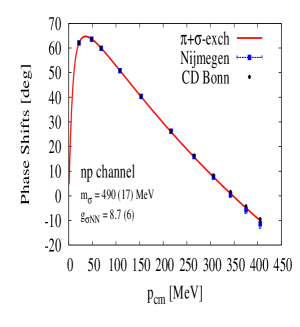
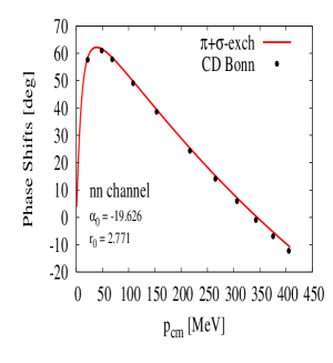
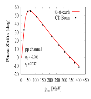
Figure 5: Renormalized phase shifts for the OBE potential with CSB OPE + $\sigma$ as a function of the c.m. momentum in the singlet ${}^{1}S_{0}$ channel. In the left panel we show the fitted $np$ phase-shift to the Nijmegen results Stoks et al. (1994). In the middle and right panels the predicted $pp(c)$ and $nn$ are depicted and compared to the CD-Bonn result Machleidt (2001).

These two problems are related at short distances through the boundary condition corresponding to the short distance connection ${\cal S}_{1}={\cal S}_{2}$

$$R_{2}\,\frac{u^{\prime}_{2}(r_{c})}{u_{2}(r_{c})}=\log{\frac{R_{1}}{R_{2}}}+R_{1}\frac{u^{\prime}_{1}(r_{c})}{u_{1}(r_{c})}\,.$$ (103)

If we have only fixed the scattering length, the above condition becomes energy independent when the cut-off is small enough, which means that it can be evaluated with the zero-energy wave functions of the two-body systems $1$ and $2$. Using the superposition principle, the previous zero energy wave functions can be written as

$$u_{1}(r)=v_{1}(r)-\frac{1}{\alpha_{1}}w_{1}(r)\,,$$ (104)

$$u_{2}(r)=v_{2}(r)-\frac{1}{\alpha_{2}}w_{2}(r)\,.$$ (105)

These wave functions can be included in Eq. (103), yielding the following relation between the scattering lengths $\alpha_{1}$ and $\alpha_{2}$ of the two different problems

$$\frac{A}{\alpha_{1}}=\frac{B}{\alpha_{2}}+C+\frac{D}{\alpha_{1}\,\alpha_{2}}\,.$$ (106)

Therefore, if we make the hypothesis of Charge independence at short distances 

$${\cal S}_{np}={\cal S}_{nn}={\cal S}_{pp}={\cal S}_{pp}^{C}\,,$$ (107)

and by making use of the superposition principle, we can write

$$u_{0,np}(r) = v_{0,np}(r)-\frac{1}{\alpha_{0,np}}w_{0,np}(r)\,,$$ (108)

$$u_{0,nn}(r) = v_{0,nn}(r)-\frac{1}{\alpha_{0,nn}}w_{0,nn}(r)\,,$$ (109)

$$u_{0,pp}(r) = v_{0,pp}(r)-\frac{1}{\alpha_{0,pp}}w_{0,pp}(r)\,,$$ (110)

$$u_{0,pp}^{C}(r) = v_{0,pp}^{C}(r)-\frac{1}{\alpha_{0,pp}^{C}}w_{0,pp}^{C}(r)\,,$$ (111)

so we get the bilinear relations between all scattering lengths

$$\frac{A_{nn}}{\alpha_{nn}} = \frac{B_{nn}}{\alpha_{np}}+C_{nn}+\frac{D_{nn}}{\alpha_{nn}\,\alpha_{np}}\,,$$ (112)

$$\frac{A_{pp}}{\alpha_{pp}} = \frac{B_{pp}}{\alpha_{np}}+C_{pp}+\frac{D_{pp}}{\alpha_{pp}\,\alpha_{np}}\,,$$ (113)

$$\frac{A^{C}_{pp}}{\alpha^{C}_{pp}} = \frac{B^{C}_{pp}}{\alpha_{np}}+C^{C}_{pp}+\frac{D^{C}_{pp}}{\alpha^{C}_{pp}\,\alpha_{np}}\,,$$ (114)

etc. In Fig. 4 we show the dependence of the scattering lengths as obtained from the $np$ scattering length and the previous correlations. As can be seen, the correlations work rather well, confirming the idea that finiteness is a good criterion to implement charge independence of short distance operators. Numerical values are listed in Table 2 for the experimental value of $\alpha_{0,np}$.

It is interesting to see how the short distance connection works at finite energy and, in particular, if a given specific $NN$ channel is able to predict the phase shifts for the remaining channels. In Fig. 5 we plot the extracted $nn$ and $pp(c)$ phase shifts when the OBE parameters have been fixed from the ${}^{1}S_{0}$ Nijmegen $np$ phase shifts. We have computed these phase shifts renormalizing in the $np$ channel, i.e., fixing $\alpha_{0,np}$ as input and integrating inward the Schrödinger equation, and then using Eq. (107) we connect with the other channels. As we can see the short distance connection can be used to predict the ${}^{1}S_{0}$ phase shits for the rest of the channel with a high degree of accuracy.

VI Conclusions

In this paper we have analyzed the charge dependence and charge symmetry breaking of the $NN$ interaction. We have used the OBE model with exchange of $\pi$, $\sigma$, $\omega$ and $\rho$ mesons and we have implemented CSB by means of pion mass splitting in the OPE potential and different nucleon masses. In particular, and as in previous works, we have selected the ${}^{1}S_{0}$ $np$ channel to fit scalar meson parameters, $m_{\sigma}$ and $g_{\sigma NN}$, as well as vector meson couplings, $g_{\omega NN}$ and $f_{\rho NN}$ to the Nijmegen phase shifts Stoks et al. (1994). A fine tuning problem arises when we using the customary regular boundary condition at the origin $u(0)=0$. This problem appears in all $np$,$nn$,$pp$ and $pp(c)$ channels and large,$\sim 40\%$ , violations of $SU(3)$ values of the $g_{\omega NN}$ coupling constant are needed. Traditionally a great amount of effects such as multi-meson exchanges have been essential to explain the differences in phase shifts and threshold parameters for all $np$,$nn$,$pp$ and $pp(c)$ channels Li and Machleidt (1998a, b); Machleidt (2001) or the role played by $\rho-\omega$ McNamee et al. (1975); Coon et al. (1977); Friar and Gibson (1978) and/or $\pi-\eta$ Piekarewicz (1993) mixing were invoked. These standard approaches need very precise information on the interaction at all distances.

However, once we admit incomplete knowledge of the interaction at short distances, it is possible to sidestep the problem of fine tuning by imposing a renormalization condition; at any stage of the calculation the scattering length is always kept fixed. This renormalization approach embodies short distance insensitivity. As a consequence, in the Charge Independent case, one can confortably take the experimental and/or SU(3) values for vector meson couplings. For the same reason we can only hope to quantitatively describe the relative changes due to the Charge Symmetry Breaking of the interaction at long distances. These considerations alone allow to extract some universal information on the symmetry breaking pattern where the $np$, $nn$ and $pp$ channels look very much the same at all energies even though the potentials are different and are indeed CSB. We have used a short distance condition to relate the renormalized $np$ channel with the others $nn$, $pp$ and $pp(c)$. This short distance connection is so far an assumption based on finiteness but we have seen that reasonable results are obtained for low energy parameters and phase shifts. Our predictions for $(\Delta\alpha_{CIB},\ \Delta r_{CIB})$ and $(\Delta\alpha_{CSB},\ \Delta r_{CSB})$ are compatible with the empirical one within the error estimation. This is in fact a remarkable result: all channels are generated with just one scattering length, say $np$, and the long distance components of the potential where the CSB is, via physical pion and nucleon masses, explicitly built in. Our result is compatible with the interpretation that (relative) CSB sits at large distances. The absolute CSB is in a sense as uncertain as the short distance components of the NN force itself and cannot be determined independently of the Charge Invariant interaction.

Appendix A Proton-proton fusion

We would like to analyze further consequences of the short distance connection assumed by Eq. (107). An interesting process is the proton-proton fusion reaction $pp\to d\ e^{+}\nu_{e}$ which is of central importance to stellar physics and neutrino astro-physics. In fact, it is the dominant solar neutrino source. The temperature in the Sun core is around $T_{c}=15\times 10^{6}K$ which means that we have protons of momentum $p\sim(2m_{p}T_{c})^{1/2}\sim 1.1\,{\rm MeV}$. At these low energies, the reaction is dominated by the ${}^{1}S_{0}\to d$ nuclear transition. The Gamow-Teller (GT) matrix element for this process (without MECs) is given by,

$$A_{S}M_{GT}=\int_{0}^{\infty}{\rm dr}\ u_{\gamma}(r)u_{0,pp}(r)$$ (115)

where $u_{0,pp}$ is the zero energy reduced wave function for the $pp(c)$ system which can be related with the $np$ problem by Eq. (107). Then taking $\alpha_{0,np}$ as input and integrating in we can calculate $u_{0,pp}$. For deuteron we take as a first approximation the normalized bound state,

$$u_{\gamma}(r)\to A_{S}e^{-\gamma_{d}r}\,,$$ (116)

with $\gamma_{d}=0.2316{\rm fm}^{-1}$ and integrate inward the Schrödinger equation with negative energy $E=-\gamma_{d}^{2}/M_{np}$. We obtain a value $M_{GT}=5.189\,{\rm fm}$ to be compared to a more sophisticated one Park et al. (1998) using Argonne $V18$ wave functions $M_{GT}|_{AV18}=4.859\,{\rm fm}$.

Figure 6: Dependence of the $pp$ fusion Gamow-Teller matrix element (in ${\rm fm}$) depending on the singlet $np$ inverse scattering length $1/\alpha_{0}$ (in ${\rm fm}^{-1}$) using the short distance connection Eq. (107).

In Fig. 6 we show the GT matrix element correlation with the $np$ scattering length compared with the AV18 calculation. Of course we have not included the tensor force which mixed $S$ and $D$ waves in the calculation of the deuteron. However we can appreciate that our numbers are not very far from much more elaborate calculations Park et al. (1998).

References

- Wilkinson (1969) D. H. e. Wilkinson, Isospin in Nuclear Physics (New York ;John Wiley and Sons, Inc. (1969)., 1969).
- Miller et al. (1990) G. A. Miller, B. M. K. Nefkens, and I. Slaus, Phys. Rept. 194, 1 (1990).
- Miller et al. (2006) G. A. Miller, A. K. Opper, and E. J. Stephenson, Ann. Rev. Nucl. Part. Sci. 56, 253 (2006), eprint nucl-ex/0602021.
- Machleidt and Slaus (2001) R. Machleidt and I. Slaus, J. Phys. G27, R69 (2001), eprint nucl-th/0101056.
- Machleidt et al. (1987) R. Machleidt, K. Holinde, and C. Elster, Phys. Rept. 149, 1 (1987).
- Cheung and Machleidt (1986) C. Y. Cheung and R. Machleidt, Phys. Rev. C34, 1181 (1986).
- Stoks et al. (1994) V. G. J. Stoks, R. A. M. Klomp, C. P. F. Terheggen, and J. J. de Swart, Phys. Rev. C49, 2950 (1994), eprint nucl-th/9406039.
- Wiringa et al. (1995) R. B. Wiringa, V. G. J. Stoks, and R. Schiavilla, Phys. Rev. C51, 38 (1995), eprint nucl-th/9408016.
- Li and Machleidt (1998a) G.-Q. Li and R. Machleidt, Phys. Rev. C58, 1393 (1998a), eprint nucl-th/9804023.
- Li and Machleidt (1998b) G.-Q. Li and R. Machleidt, Phys. Rev. C58, 3153 (1998b), eprint nucl-th/9807080.
- Machleidt (2001) R. Machleidt, Phys. Rev. C63, 024001 (2001), eprint nucl-th/0006014.
- Machleidt and Muther (2001) R. Machleidt and H. Muther, Phys. Rev. C63, 034005 (2001), eprint nucl-th/0011057.
- Biswas et al. (2008) S. Biswas, P. Roy, and A. K. Dutt-Mazumder, Phys. Rev. C78, 045207 (2008), eprint 0805.3046.
- Hamilton and Oades (1984) J. Hamilton and G. C. Oades, Nucl. Phys. A424, 447 (1984).
- Piekarewicz (1993) J. Piekarewicz, Phys. Rev. C48, 1555 (1993), eprint nucl-th/9303005.
- Howell (2008) C. R. Howell (2008), eprint 0805.1177.
- Gardestig (2009) A. Gardestig, J. Phys. G36, 053001 (2009), eprint 0904.2787.
- Fonseca et al. (2009) A. C. Fonseca, R. Machleidt, and G. A. Miller, Phys. Rev. C80, 027001 (2009), eprint 0907.0215.
- Calle Cordon and Ruiz Arriola (2010) A. Calle Cordon and E. Ruiz Arriola, Phys. Rev. C81, 044002 (2010), eprint 0905.4933.
- Calle Cordon and Ruiz Arriola (2008) A. Calle Cordon and E. Ruiz Arriola, AIP Conf. Proc. 1030, 334 (2008), eprint 0804.2350.
- Kong and Ravndal (1999) X. Kong and F. Ravndal, Phys. Lett. B450, 320 (1999), eprint nucl-th/9811076.
- Kong and Ravndal (2000) X. Kong and F. Ravndal, Nucl. Phys. A665, 137 (2000), eprint hep-ph/9903523.
- Gegelia (2004) J. Gegelia, Eur. Phys. J. A19, 355 (2004), eprint nucl-th/0310012.
- Walzl et al. (2001) M. Walzl, U. G. Meissner, and E. Epelbaum, Nucl. Phys. A693, 663 (2001), eprint nucl-th/0010019.
- Epelbaum and Meissner (2005) E. Epelbaum and U.-G. Meissner, Phys. Rev. C72, 044001 (2005), eprint nucl-th/0502052.
- Ando et al. (2007) S.-i. Ando, J. W. Shin, C. H. Hyun, and S. W. Hong, Phys. Rev. C76, 064001 (2007), eprint 0704.2312.
- Bethe (1949) H. A. Bethe, Phys. Rev. 76, 38 (1949).
- de Swart et al. (1997) J. J. de Swart, M. C. M. Rentmeester, and R. G. E. Timmermans, PiN Newslett. 13, 96 (1997), eprint nucl-th/9802084.
- Lepage (1997) G. P. Lepage (1997), eprint nucl-th/9706029.
- Phillips and Cohen (1997) D. R. Phillips and T. D. Cohen, Phys. Lett. B390, 7 (1997), eprint nucl-th/9607048.
- Entem et al. (2008) D. R. Entem, E. Ruiz Arriola, M. Pavon Valderrama, and R. Machleidt, Phys. Rev. C77, 044006 (2008), eprint 0709.2770.
- Pavon Valderrama and Ruiz Arriola (2009) M. Pavon Valderrama and E. Ruiz Arriola, Phys. Rev. C80, 024001 (2009), eprint 0904.1120.
- Abramowitz and Stegun (1964) M. Abramowitz and I. A. Stegun, Handbook of Mathematical Functions with Formulas, Graphs, and Mathematical Tables (Dover, New York, 1964), ninth dover printing, tenth gpo printing ed., ISBN 0-486-61272-4.
- Park et al. (1998) T.-S. Park, K. Kubodera, D.-P. Min, and M. Rho, Astrophys. J. 507, 443 (1998), eprint astro-ph/9804144.
- McNamee et al. (1975) P. C. McNamee, M. D. Scadron, and S. A. Coon, Nucl. Phys. A249, 483 (1975).
- Coon et al. (1977) S. A. Coon, M. D. Scadron, and P. C. Mcnamee, Nucl. Phys. A287, 381 (1977).
- Friar and Gibson (1978) J. L. Friar and B. F. Gibson, Phys. Rev. C17, 1752 (1978).