Latent diffusion models for survival analysis

Abstract

We consider Bayesian hierarchical models for survival analysis, where the survival times are modeled through an underlying diffusion process which determines the hazard rate. We show how these models can be efficiently treated by means of Markov chain Monte Carlo techniques.

and

1 Introduction

Diffusion processes have found many applications in the modeling of continuous-time phenomena, for problems related to a variety of scientific areas, ranging from economics to biology, from physics to engineering. Here, we use diffusion processes as building blocks for the definition of models for survival and event history analysis. This idea is not new (see, e.g., the reviews in Aalen and Gjessing (2001, 2004)). However, in this paper, we are able to considerably extend the flexibility of the diffusion models used, by adopting powerful Markov chain Monte Carlo techniques.

Diffusion models for survival analysis have been proposed because, as summarized in Aalen and Gjessing (2004), “when modelling survival data it may be of interest to imagine an underlying process leading up to the event in question.” Such a process might, for example, represent the development of a disease. Two types of models have been considered in the literature: models where the event happens when a diffusion process hits some barrier and models where the hazard rate is some suitable function of the diffusion. For the former type of model, we refer the reader to Aalen and Gjessing (2001), Aalen, Borgan and Gjessing (2008) and references therein. Here, we are interested in the latter. Woodbury and Manton (1977) proposed a model where the hazard rate is a quadratic function of an Ornstein–Uhlenbeck diffusion process. This model has since been considered by several authors, including Myers (1981), Yashin (1985), Yashin and Vaupel (1986) and Aalen and Gjessing (2004). For given values of the parameters of the Ornstein–Uhlenbeck process, survival distributions and hazards are studied. Myers (1981) focuses on survival distributions conditioned on initial covariate values; Yashin (1985) and Yashin and Vaupel (1986) use hazards based on quadratic functions of Ornstein–Uhlenbeck processes in order to model heterogeneity among groups and individuals, and to study the relative hazard functions and survival distributions; Aalen and Gjessing (2004) derives quasi-stationary distributions. Obtaining such analytical results for hazard functions other than quadratic functions, or for more complex diffusion processes, is not feasible.

In our paper, we adopt a Bayesian approach and show how these models can be efficiently treated by means of Markov chain Monte Carlo techniques for general choices of diffusion processes and hazard functions. For instance, by the proposed methods, it is possible to deal with latent diffusion models which are stochastic perturbations of common survival models. We also consider the case of multiple groups of observations, typical of clinical trials, and we show how to efficiently deal with covariates. We illustrate the methods via simulation studies and applications to real-world data.

It should be mentioned that other classes of Bayesian nonparametric and semi-parametric models for survival analysis have been proposed in the literature. Among the most important, we mention the models based on neutral to the right random probabilities, whose cumulative hazard rates are processes with independent increments (see Doksum (1974) and Ferguson (1974) for the definition and properties of these random measures, and, e.g., Susarla and Van Ryzin (1976), Kalbfleisch (1978), Ferguson and Phadia (1979), Hjort (1990) and Damien and Walker (2002) for applications in survival analysis), and all models falling within the framework of multiplicative intensity models, whose hazard rates are mixtures of known kernels where the mixing measure is a weighted gamma process (see Dykstra and Laud (1981), Lo and Weng (1989), Ishwaran and James (2004) and references therein).

The paper is organized as follows. In Section 2, we recall the essentials of diffusion processes and introduce the model; we also outline how, in the described framework, it is possible to consider stochastic perturbations of common survival models. In Section 3, we describe the MCMC scheme and gives the details of a suitable Hastings-within-Gibbs algorithm, showing its implementation by means of a toy example. In Section 4, we present improved versions of the algorithm, based on reparametrizations of the model. In Section 5, we discuss a straightforward generalization of the framework developed in the previous sections and deal with the case of multiple groups of observations; this is also illustrated by application to a data set from a clinical trial, one that has been considered in a number of papers in the context of survival analysis, the famous paper by Cox (1972) being among the earliest. In Section 6, we describe how covariates can be efficiently included in the proposed models and give an illustrative application to the lung cancer data set analyzed by Muers, Shevlin and Brown (1996). Finally, in Sections 7 and 8, we discuss possible extensions of the models considered.

2 Latent diffusion models

Let $\Theta$ be a random variable with values in $\mathbb{R}^{d}$. Denote by $C([0,\infty),\mathbb{R})$ the space of continuous functions from $[0,\infty)$ to $\mathbb{R}$ and by $\mathcal{C}$ its cylinder $\sigma$-algebra. Given $\Theta=\theta$, consider the scalar diffusion process $X=\{X_{t}\colon\ t\geq 0\}$, solution of a stochastic differential equation (SDE) of the form

$$\mathrm{d}X_{t} = \beta(X_{t},\theta)\,\mathrm{d}t+\sigma\,\mathrm{d}B_{t},\qquad t\geq 0,$$

$$X_{0} = x_{0},$$

driven by the standard scalar Brownian motion $B=\{B_{t}\colon\ t\geq 0\}$. The Brownian motion $B$ and the diffusion process $X$ are random elements of $(C([0,\infty),\mathbb{R}),\mathcal{C})$. The diffusion coefficient $\sigma$ is assumed constant and known, for the moment. The more technically difficult case of unknown $\sigma$ is postponed to Section 7. The drift $\beta(x,\theta)$ is assumed to be jointly measurable in $x$ and $\theta$, and to satisfy the regularity conditions (locally Lipschitz, with linear growth bound) that guarantee the existence of a weakly unique global solution to (2). See, for example Rogers and Williams (2000), Chapter V.24.

Let $\mathbb{W}_{\sigma}$ be the law of $\sigma B$ and, for a given $\theta$, denote by $\mathbb{P}_{\theta}$ the law of the diffusion $X$, solution of (2). By Girsanov’s theorem, the Radon–Nikodym derivative of $\mathbb{P}_{\theta}$ with respect to $\mathbb{W}_{\sigma}$ is given by

$$\frac{\mathrm{d}\mathbb{P}_{\theta}}{\mathrm{d}\mathbb{W}_{\sigma}}(x)=\exp\biggl{\{}\int_{0}^{\infty}\frac{\beta(x_{t},\theta)}{\sigma^{2}}\,\mathrm{d}x_{t}-\frac{1}{2}\int_{0}^{\infty}\frac{\beta(x_{t},\theta)^{2}}{\sigma^{2}}\,\mathrm{d}t\biggr{\}},$$

where $x$ is an element of $(C([0,\infty),\mathbb{R}),\mathcal{C})$. See, for example, Rogers and Williams (2000), Chapter V.27.

Similarly, for a finite $T$, denote by $C([0,T],\mathbb{R})$ the space of continuous functions from $[0,T]$ to $\mathbb{R}$ and by $\mathcal{C}^{T}$ its cylinder $\sigma$-algebra. Then, $B_{[0,T]}:=\{B_{t}\colon\ 0\leq t\leq T\}$ and $X_{[0,T]}=\{X_{t}\colon\ 0\leq t\leq T\}$ are random elements of $(C([0,T],\mathbb{R}),\mathcal{C}^{T})$. Let $\mathbb{W}_{T,\sigma}$ be the law of $\sigma B_{[0,T]}$ and, for a given $\theta$, denote by $\mathbb{P}_{T,\theta}$ the law of $X_{[0,T]}$. Then, by Girsanov’s theorem, the Radon–Nikodym derivative of $\mathbb{P}_{T,\theta}$ with respect to $\mathbb{W}_{T,\sigma}$ is given by

$$\frac{\mathrm{d}\mathbb{P}_{T,\theta}}{\mathrm{d}\mathbb{W}_{T,\sigma}}\bigl{(}x_{[0,T]}\bigr{)}=\exp\biggl{\{}\int_{0}^{T}\frac{\beta(x_{t},\theta)}{\sigma^{2}}\,\mathrm{d}x_{t}-\frac{1}{2}\int_{0}^{T}\frac{\beta(x_{t},\theta)^{2}}{\sigma^{2}}\,\mathrm{d}t\biggr{\}}$$ (2)

and, for each $T$, the measures $\mathbb{P}_{T,\theta}$ are absolutely continuous.

Given the diffusion $X$, let us consider the random distribution function $F_{X,h}$ on $[0,\infty)$, defined as

$$F_{X,h}(t):=1-\exp\biggl{\{}-\int_{0}^{t}h(X_{s})\,\mathrm{d}s\biggr{\}},\qquad t\geq 0,$$ (3)

where $h(\cdot)$ is some suitable non-negative and continuous function with $\int_{0}^{\infty}h(X_{s})\,\mathrm{d}s=\infty$ almost surely. The function $h(\cdot)$ plays the role of the hazard function and $h(X_{t})$ is the random hazard rate at time $t$ associated with the random distribution $F_{X,h}$.

Two features of the random measure $F_{X,h}$ have to be noted. The first is that the hazard inherits the Markov property of the diffusion process so that the hazard at a future time $t^{\prime}$ depends only on the hazard at the present time $t$. Indeed, the Markov property seems a sensible choice to make at the level of the hazard. The second is that the cumulative hazard is a process with positively correlated increments, being the integral of a continuous process. The latter feature is natural in many contexts and it introduces to the model a concern with the stochastic process that clearly must lie behind the occurrence of events. In words, a high increment of the cumulative hazard over the time interval $[t,t^{\prime}]$ means that the underlying stochastic process has reached a region of high risk and this is likely to yield a high increment of the cumulative hazard over a close (disjoint) time interval. The strength of this positive correlation, and thus the smoothness of the cumulative hazard, depends on the choice of the hazard function $h$ and of the diffusion process $X$: the rougher the diffusion, the weaker the correlation, and vice versa; see also the comments in Section 8. Note that the property we have just highlighted differentiates the models we are considering from models based on neutral to the right random probabilities, whose cumulative hazards are processes with independent increments and thus have an erratic behaviour.

Let us now consider a sequence of event times $Y_{1},Y_{2},\ldots$ which are, conditionally on $F_{X,h}$, independent and identically distributed (i.i.d.) with common distribution $F_{X,h}$. From (3), it follows that the distribution of $Y_{1},\ldots,Y_{n}$, given $X=x$, has density, with respect to the $n$-dimensional Lebesgue measure $\mathcal{L}^{n}$, given by

$$l(y_{1},\ldots,y_{n}|x):=\Biggl{[}\prod_{j=1}^{n}h(x_{y_{j}})\Biggr{]}\exp\Biggl{\{}-\sum_{j=1}^{n}\int_{0}^{y_{j}}h(x_{t})\,\mathrm{d}t\Biggr{\}}.$$ (4)

Censored observations can easily be dealt with in this setting. In the present paper, we shall restrict our attention to independent right-censored schemes. If we let $(y_{1},\ldots,y_{m})$ be the observed event times and let $(y_{m+1}\!+,\ldots,y_{n}\!+)$ be the right-censored event times, then the likelihood becomes

$$l(y_{1},\ldots,y_{m},y_{m+1}\!+,\ldots,y_{n}\!+|x)$$

$$\quad=\Biggl{[}\prod_{j=1}^{m}h(x_{y_{j}})\Biggr{]}\exp\Biggl{\{}-\sum_{j=1}^{m}\int_{0}^{y_{j}}h(x_{t})\,\mathrm{d}t-\sum_{j=m+1}^{n}\int_{0}^{y_{j}+}h(x_{t})\,\mathrm{d}t\Biggr{\}}.$$

We are thus considering a latent diffusion model for survival analysis, where the survival times are modeled via an underlying diffusion process which determines the hazard rate. As highlighted by Aalen and Gjessing (2004), this model can also be interpreted as a random barrier hitting model. Indeed, the event occurs when the cumulative hazard strikes a random barrier $R$, which is exponentially distributed with mean 1 and is stochastically independent of $X$.

2.1 Stochastic perturbations of common survival models

In the framework we have described, one possibility is to consider stochastic perturbations of common survival models. Heuristically, the idea is that if we can express the hazard $r(t)$ of a given model as a solution of an ordinary differential equation $\frac{\mathrm{d}r(t)}{\mathrm{d}t}=g(r(t))$ for some suitable function $g$, then we may be able to use $g$, or some modification of it, to model the drift of an SDE. Starting from this SDE, we can thus consider a latent diffusion model whose hazard function is a stochastic perturbation of $r(t)$.

We shall illustrate this by means of some examples. The simplest case is offered by the Gompertz model. The Gompertz hazard $r(t)=\beta\exp\{\alpha t\}$, for $\alpha,\beta>0$, is a solution of the ordinary differential equation $\frac{\mathrm{d}r(t)}{\mathrm{d}t}=g(r(t))=\alpha r(t)$. Consider, thus, the latent diffusion model based on the SDE having drift $g(X_{t})=\theta X_{t}$ for $\theta>0$,

$$\mathrm{d}X_{t}=\theta X_{t}\,\mathrm{d}t+\sigma\,\mathrm{d}B_{t},\qquad t\geq 0,\qquad X_{0}=x_{0}>0,$$ (5)

and with hazard function $h(u)=|u|$. For $\sigma=0$, the SDE (5) reduces to the ordinary differential equation written above, for which the Gompertz hazard is a solution, and the latent diffusion model reduces to the Gompertz model. Hence, the latent diffusion model based on the SDE (5) with hazard function $h(u)=|u|$ can be seen as a stochastic perturbation around a central Gompertz model. This constitutes a simple example of a latent diffusion model, for which the law of $X_{t}$, and thus also the law of the hazard, is known. In the other examples we shall now give, the SDE cannot be explicitly solved, but the latent diffusion models based on them can be treated by the techniques described in the present paper.

Let us consider the Weibull model, whose hazard $r(t)=\alpha\beta t^{\alpha-1}$ for $\alpha,\beta>0$ is a non-trivial solution of the ordinary differential equation $\frac{\mathrm{d}r(t)}{\mathrm{d}t}=g(r(t))=\gamma r(t)^{(\alpha-2)/(\alpha-1)}$. Consider, thus, the latent diffusion model based on the SDE

$$\mathrm{d}X_{t}=\theta_{1}(\operatorname{sign}(X_{t}))|X_{t}|^{\theta_{2}}\,\mathrm{d}t+\sigma\,\mathrm{d}B_{t},\qquad t\geq 0,\qquad X_{0}=x_{0}>0,$$ (6)

where

$$\operatorname{sign}(u)=\cases{1,&\quad\mbox{if} $u>0,$\cr-1,&\quad\mbox{if} $u<0,$\cr 0,&\quad\mbox{if} $u=0,$}$$

and with hazard function $h(u)=|u|$. For $\sigma=0$, the SDE (6) reduces to the ordinary differential equation written above, for which the Weibull hazard is a solution ($\theta_{2}$ here plays the role of $(\alpha-2)/(\alpha-1)$). Hence, the latent diffusion model based on the SDE (6), with hazard function $h(u)=|u|$, can be seen as a stochastic perturbation around a central Weibull model. For values of $\theta_{2}$ in the interval $(0,1)$, which correspond to $\alpha>2$, the SDE (6) has a non-explosive solution. This solution is weakly unique (see, e.g., Stroock and Varadhan (2006)). In Sections 5.1 and 6.1, we shall implement this latent diffusion model in some illustrative applications to real-world data.

Using the simple idea outlined above, it is possible to develop other latent diffusion models, such as stochastic perturbations of log-logistic models and exponential-power models. The log-logistic hazard ($r(t)=\alpha\beta t^{\alpha-1}/(1+\beta t^{\alpha})$ for $\alpha,\beta>0$) and the exponential-power hazard ($r(t)=\alpha\beta^{\alpha}t^{\alpha-1}\exp\{(\beta t)^{\alpha}\}$ for $\alpha,\beta>0$) can, in fact, be written as solutions of $\frac{\mathrm{d}r(t)}{\mathrm{d}t}=g(r(t))$ for suitable functions $g$ (when $\alpha<1$ for the log-logistic and $\alpha>1$ for the exponential-power). Let us give a further example, which generalizes the Pareto model. The Pareto hazard $r(t)=\alpha/t$, for $\alpha>0$ and $t\geq\lambda>0$, is a solution of the equation $\frac{\mathrm{d}r(t)}{\mathrm{d}t}=g(r(t))=-\frac{1}{\alpha}[r(t)]^{2}$. Now, the SDE having drift $g(X_{t})=-\theta X_{t}^{2}$, for $\theta>0$,

$$\mathrm{d}X_{t}=-\theta X_{t}^{2}\,\mathrm{d}t+\sigma\,\mathrm{d}B_{t},\qquad t\geq\lambda>0,\qquad X_{\lambda}=x_{\lambda}>0,$$ (7)

provides a stochastic perturbation around the Pareto hazard, but, unfortunately, this SDE cannot be used for our purposes since it has an explosive solution. On the other hand, we can modify (7), for example, by inclusion of $X_{t}$ in the diffusion coefficient, in order to obtain another SDE,

$$\mathrm{d}X_{t}=-\theta X_{t}^{2}\,\mathrm{d}t+\sigma X_{t}\,\mathrm{d}B_{t},\qquad t\geq\lambda>0,\qquad X_{\lambda}=x_{\lambda}>0,$$ (8)

that also provides a stochastic perturbation around the Pareto hazard, but has a non-explosive solution. The latter SDE can thus be transformed into one of constant diffusion coefficient, which can, in turn, be used in the latent diffusion model. Note that the solution of (8), and that of the corresponding SDE with constant coefficient, are almost surely positive and so we can take as hazard function $h(\cdot)$ the identity function, obtaining a particularly natural perturbation of the Pareto. It is worth recalling that an SDE with general diffusion coefficient $\sigma(X_{t},\theta)$,

$$\mathrm{d}X_{t}=\beta(X_{t},\theta)\,\mathrm{d}t+\sigma(X_{t},\theta)\,\mathrm{d}B_{t},\qquad t\geq 0,\qquad X_{0}=x_{0},$$

can, in fact, be transformed into an SDE of unit diffusion coefficient for the process $Y$, by applying the 1–1 transformation $X_{t}\to\eta(X_{t};\theta)=:Y_{t}$, where $\eta(x;\theta)=\int^{x}\frac{1}{\sigma(z;\theta)}\,\mathrm{d}z$ is any anti-derivative of $\sigma^{-1}(\cdot;\theta)$ (we are assuming that $\sigma(x,\theta)$ is differentiable for any $x\in C([0,\infty),\mathbb{R})$); see, for example, Beskos et al. (2006). This approach opens up to a number of possible stochastic perturbations of commonly used hazards.

3 Markov chain Monte Carlo methods for latent diffusion models

Let $p_{\Theta}(\theta)$ be the prior density, with respect to $\mathcal{L}^{d}$, of the $d$-dimensional parameter $\Theta$ which appears in the drift of the diffusion process $X$, solution of (2). Fix a finite time horizon $T$ of interest, with $T\geq y_{[n]}$, where $y_{[n]}:=\max\{y_{1},\ldots,y_{n}\}$. The choice of $T$ will be discussed in Section 4. Then, the joint posterior distribution of $\Theta$ and $X_{[0,T]}$ has density, with respect to the product measure $\mathcal{L}^{d}\otimes\mathbb{W}_{T,\sigma}$, given by

$$\pi\bigl{(}\theta,x_{[0,T]}|y_{1},\ldots,y_{n}\bigr{)}=Cp_{\Theta}(\theta)g\bigl{(}x_{[0,T]}|\theta\bigr{)}l\bigl{(}y_{1},\ldots,y_{n}|x_{[0,y_{[n]}]}\bigr{)},$$ (9)

where $C$ is a normalizing constant and $g(x_{[0,T]}|\theta):=\frac{\mathrm{d}\mathbb{P}_{T,\theta}}{\mathrm{d}\mathbb{W}_{T,\sigma}}(x)$ is given by Girsanov’s formula (2).

A Gibbs sampling algorithm for sampling from (9) alternates between

1. [1.]

2. simulation of $\Theta$, conditional on the observations and the current path of $X_{[0,T]}$;

3. simulation of $X_{[0,T]}$, conditional on the observations and the current value of $\Theta$.

Note that the parameter $\Theta$ and the observations $Y_{1},\ldots,Y_{n}$ are conditionally independent, given the non-observed process $X_{[0,T]}$. In particular, from (9), the conditional distribution of $\Theta$ given $X_{[0,T]}$ has density, with respect to $\mathcal{L}^{d}$, proportional to $p_{\Theta}(\theta)g(x_{[0,T]}|\theta)$. The update of the parameter is particularly straightforward when a conjugate prior $p_{\Theta}(\theta)$ is chosen so that it is possible to analytically derive the conditional distribution of $\Theta$ given $X_{[0,T]}$ and sample directly from it. The second step is computationally more demanding. From (9), the conditional distribution of $X_{[0,T]}$, given parameter and observations, has density, with respect to $\mathbb{W}_{T,\sigma}$, proportional to $g(x_{[0,T]}|\theta)l(y_{1},\ldots,y_{n}|x)$ and cannot be sampled directly. An appropriate Metropolis–Hastings step is thus required.

Implementation of the algorithm will necessary involve a discretization of the diffusion sample path. When the SDE cannot be solved, it is possible to use Euler–Maruyama approximation; see, for example, Chapter 9 in Kloeden and Platen (1992). Alternatively, it may be possible to simulate the diffusion path by means of the exact algorithm described in Beskos et al. (2006), thus avoiding approximation errors.

3.1 Hastings-within-Gibbs algorithm for a latent diffusion model

We now give the details of the Hastings-within-Gibbs algorithm for latent diffusion models.

Just as an example, consider a latent diffusion model with base diffusion which is solution of the SDE

$$\mathrm{d}X_{t}=\theta^{\mathsf{T}}f(X_{t})\,\mathrm{d}t+\sigma\,\mathrm{d}B_{t},\qquad t\geq 0,\qquad X_{0}=x_{0},$$ (10)

with $\theta^{\mathsf{T}}=(\theta_{1},\ldots,\theta_{d})$ and $f(x)^{\mathsf{T}}=(f_{1}(x),\ldots,f_{d}(x))$, where $f_{i}(x)$ is some real-valued function for $i=1,\ldots,d$. Let the drift $\theta^{\mathsf{T}}f(x)$ be such that the regularity conditions mentioned in Section 2 are satisfied. Let the prior for $\Theta=(\Theta_{1},\ldots,\Theta_{d})$ be multivariate Gaussian with mean vector and variance matrix, respectively, given by

$$\mu=\left[\matrix{\mu_{1}\cr\mu_{2}\cr\vdots\cr\mu_{d}}\right]\quad\mbox{and}\quad\Sigma=\left[\matrix{\lambda_{11}&\lambda_{12}&\cdots&\lambda_{1d}\cr\lambda_{12}&\lambda_{22}&\cdots&\lambda_{2d}\cr\vdots&\vdots&\ddots&\vdots\cr\lambda_{1d}&\lambda_{2d}&\cdots&\lambda_{dd}}\right]^{-1}.$$

Then, the distribution of $\Theta$, given the diffusion $X_{[0,T]}=x_{[0,T]}$, is still Gaussian, with mean and covariance matrix, respectively, given by

$$\mu_{x}=\Sigma_{x}\left[\matrix{S_{1}\cr S_{2}\cr\vdots\cr S_{d}}\right]\quad\mbox{and}\quad\Sigma_{x}=\left[\matrix{L_{11}&L_{12}&\cdots&L_{1d}\cr L_{12}&L_{22}&\cdots&L_{2d}\cr\vdots&\vdots&\ddots&\vdots\cr L_{1d}&L_{2d}&\cdots&L_{dd}}\right]^{-1},$$ (11)

where, for $i=1,\ldots,d$ and $j=1,\ldots,d$,

$$S_{i} := \frac{1}{\sigma^{2}}\int_{0}^{T}f_{i}(x_{t})\,\mathrm{d}x_{t}+\sum_{j=1}^{d}\lambda_{ij}\mu_{j},\qquad L_{ij}:=\frac{1}{\sigma^{2}}\int_{0}^{T}f_{i}(x_{t})f_{j}(x_{t})\,\mathrm{d}t+\lambda_{ij}.$$

The update of $\Theta$ can thus be performed by sampling directly from this conditional distribution.

The update of the diffusion $X_{[0,T]}$ is less straightforward and requires an appropriate Metropolis–Hastings step. It is possible, for example, to carry out an independence sampler with proposal distribution given by a Brownian motion starting at $x_{0}$. To improve the acceptance rate of the move that updates the diffusion path, we apply the following updating strategy. Let $0=t_{1}<\cdots<t_{m}=T$. Instead of proposing a new diffusion path on the whole interval $[0,T]$, we propose to change the trajectory only on a subinterval $[t_{i},t_{i+2}]$, keeping the rest of the diffusion fixed. To ensure continuity of the diffusion path, the proposal distribution for the new trajectory on the subinterval $[t_{i},t_{i+2}]$ is a Brownian bridge $\mathit{BB}_{[t_{i},t_{i+2}]}(x_{t_{i}},x_{t_{i+2}})=\{\mathit{BB}_{t}(x_{t_{i}},x_{t_{i+2}})\colon\ t_{i}\leq t\leq t_{i+2}\}$, having as starting and ending points, respectively, the values $X_{t_{i}}=x_{t_{i}}$ and $X_{t_{i+2}}=x_{t_{i+2}}$ of the current diffusion. The proposed diffusion path $x^{*}_{[0,T]}$ is then given by $\{x^{*}_{t}=1(t\notin[t_{i},t_{i+2}])x_{t}+1(t\in[t_{i},t_{i+2}])bb_{t}(x_{t_{i}},x_{t_{i+2}})\colon\ t\in[0,T]\}$, where $\mathit{bb}_{t}(x_{t_{i}},x_{t_{i+2}})$ is the realization of the Brownian bridge $\mathit{BB}_{[t_{i},t_{i+2}]}(x_{t_{i}},x_{t_{i+2}})$. This move is accepted with probability

$$1\wedge\frac{g(\mathit{bb}_{[t_{i},t_{i+2}]}(x_{t_{i}},x_{t_{i+2}})|\theta)}{g(x_{[t_{i},t_{i+2}]}|\theta)}\frac{l(y_{1},\ldots,y_{n}|x_{[0,y_{[n]}]}^{*})}{l(y_{1},\ldots,y_{n}|x_{[0,y_{[n]}]})},$$ (12)

where $g(x_{[t_{i},t_{i+2}]}|\theta)$ is given by Girsanov’s formula restricted to the interval $[t_{i},t_{i+2}]$, that is,

$$g\bigl{(}x_{[t_{i},t_{i+2}]}|\theta\bigr{)}=\exp\biggl{\{}\int_{t_{i}}^{t_{i+2}}\frac{\theta^{\mathsf{T}}f(X_{t})}{\sigma^{2}}\,\mathrm{d}x_{t}-\frac{1}{2}\int_{t_{i}}^{t_{i+2}}\frac{(\theta^{\mathsf{T}}f(X_{t}))^{2}}{\sigma^{2}}\,\mathrm{d}t\biggr{\}}.$$

The procedure is iterated for $i=1,\ldots,m-3$. Note that the different blocks $[t_{i},t_{i+2}]$ overlap so that there are no time instants where the diffusion is kept fixed. For the same reason, the last block $[t_{m-2},T]$ is updated by means of a Brownian motion $B_{[t_{m-2},T]}(x_{t_{m-2}})$ starting at $X_{t_{m-2}}=x_{t_{m-2}}$ so that the value of the diffusion at $T$ may vary. The acceptance coefficient of the move that updates the last block is the same as in (12), with $[t_{i},t_{i+2}]=[t_{m-2},T]$ and $b_{[t_{m-2},T]}(x_{t_{m-2}})$ in place of $\mathit{bb}_{[t_{i},t_{i+2}]}(x_{t_{i}},x_{t_{i+2}})$, where $b_{[t_{m-2},T]}(x_{t_{m-2}})$ is the realization of the Brownian motion $B_{[t_{m-2},T]}(x_{t_{m-2}})$.

This idea of updating smaller intervals at a time has been used in Shephard and Pitt (1997) for the simulation of non-Gaussian time series models and later applied for the simulation of discretely observed diffusions, for example, by Elerian, Chib and Shephard (2001).

In Section 3.2, we shall illustrate the implementation of this algorithm by means of a toy example. Note that in this section and in the following, we are considering base diffusions having drift linear in the parameter $\theta$ simply for purposes of exposition.

3.2 Implementation of the algorithm: A toy example

We show here the implementation of the algorithm described in Section 3.1, by means of a toy example. Consider the model based on the diffusion process satisfying the SDE

$$\mathrm{d}X_{t}=\theta_{1}\sin(X_{t})\,\mathrm{d}t+\theta_{2}\,\mathrm{d}t+\mathrm{d}B_{t},\qquad t\geq 0,\qquad X_{0}=2,$$ (13)

with hazard function $h(u)=u^{2}$. We simulate observations from this model for values of the parameters $\theta_{1}=-1.4$ and $\theta_{2}=-1$, and censoring time $C=0.9$. In particular, we sample one realization $x$ of the diffusion process satisfying (13), with $\theta_{1}=-1.4$ and $\theta_{2}=-1$. We then simulate 200 i.i.d. observations from the corresponding distribution $F_{x,h}=1-\exp\{-\int_{0}^{t}(x_{s})^{2}\,\mathrm{d}s\}$ and censor the observations at a common cut-off $C=0.9$. The diffusion is sampled at intervals of length $0.01$, using Euler–Maruyama approximation. Figure 1 shows the corresponding hazards (the squared diffusion) and a histogram of sampled data. The hazard function has a typical shape, first (mainly) increasing and then (mainly) decreasing.

We choose as time horizon of interest $T=1$. We then run the Hastings-within-Gibbs algorithm under the following specifications. The prior for $(\theta_{1},\theta_{2})$ is Gaussian, as in Section 3.1, with $\mu_{1}=-1.4$, $\mu_{2}=-1$, $\lambda_{11}=\lambda_{22}=1/5$ and $\lambda_{12}=0$. The starting values of the parameters are $\theta_{1}=\theta_{2}=0$ and the starting diffusion is a Brownian motion, starting at $x_{0}=2$. The diffusion path is updated on subintervals of length 0.2 at a time. The algorithm is run for 200 000 iterations and the first 2000 are discarded as burn-in.

Figure 2 shows the estimates of survival distribution, density and hazard function, based on the MCMC output, together with pointwise approximate $90\%$ highest posterior bands. The true survival distribution and hazard function are also displayed to demonstrate the good fit of the MCMC estimates. Figure 2 also shows autocorrelation functions for $\theta_{1}$ and $\theta_{2}$ series.

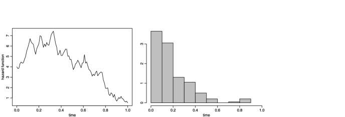
Figure 1: Left: hazard function $x^{2}$. Right: histogram of data sampled from $F_{x,x^{2}}$ with censoring at $C=0.9$.

Figure 2: Upper-left: true survival distribution $1-F_{x,x^{2}}$ (solid), together with its posterior mean (dashed) and pointwise approximate $90\%$ highest posterior bands (dotted). Upper-right: true density (solid), together with its posterior mean (dashed) and pointwise approximate $90\%$ highest posterior bands (dotted). Lower-left: true hazard function $x^{2}$ (solid), together with its posterior mean (dashed) and pointwise approximate $90\%$ highest posterior bands (dotted). Lower-right: autocorrelation functions for $\theta_{1}$ series (dotted) and $\theta_{2}$ series (dashed).

4 Reparametrizations of the latent diffusion models

The MCMC algorithm described in the previous sections might have poor mixing properties when we consider a finite-time horizon $T$ significantly larger than the maximum of the data. This problem is evident in Figure 3. This figure shows the histogram of 200 i.i.d. observations from the distribution $F_{x^{\prime},h}$, where $x^{\prime}$ is a new realization of the diffusion process satisfying the same SDE used in Section 3.2; also, the hazard function $h$ and the censoring time $C$ are the same. In this simulation, we have fixed a longer time horizon $T=1.8$ and have then run the algorithm under the same specifications of Section 3.2. Figure 3 displays autocorrelation functions for $\theta_{1}$ and $\theta_{2}$ series, which are not exponentially decreasing. With the same data set, but choosing a shorter time horizon (such as $T=1$, as in the previous section), the algorithm does not exhibit strong serial correlation in the draws of $\theta_{1}$ and $\theta_{2}$. The worsening of the mixing properties of the algorithm when $T$ becomes significantly larger than the maximum of the data was also observed for the data set simulated in Section 3.2.

To avoid this problem, we propose a modification of the algorithm which has good mixing properties, regardless of the choice of time horizon, and is, in fact, completely robust with respect to $T$. The algorithm is based on a simple reparametrization of the model. Indeed, the performance of MCMC methods, particularly when using Gibbs samplers, depends crucially on the parametrization of the unknown quantities in the hierarchical structure. The issue of reparametrization of the posterior distributions in order to improve convergence properties of the algorithms has received much attention. See, for example, Hills and Smith (1992), Gelfand, Sahu and Carlin (1995), Gelfand, Sahu and Carlin (1996) and Papaspiliopoulos, Roberts and Sköld (2003; 2007).

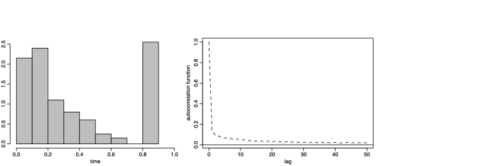
Figure 3: Left: histogram of data sampled from $F_{x^{\prime},x^{\prime 2}}$ with censoring at $C=0.9$. Right: autocorrelation functions for $\theta_{1}$ series (dotted) and $\theta_{2}$ series (dashed).

Instead of using the natural parametrization of the model in terms of $(\Theta,X)$, the so-called centered parametrization, we parametrize it in terms of $(\Theta,\widetilde{X})$, where

$$\widetilde{X}_{t}=1\bigl{(}t\leq y_{[n]}\bigr{)}X_{t}+1\bigl{(}t>y_{[n]}\bigr{)}\bigl{[}B_{t}-B_{y_{[n]}}\bigr{]},\qquad t\geq 0.$$

In the terminology used by Papaspiliopoulos, Roberts and Sköld (2003), this is called a partially non-centered parametrization, the fully non-centered parametrization being, in this case, $(\Theta,B)$. The diffusion $X$ can then be reconstructed as a function of $\Theta$, $\widetilde{X}$ and $y_{1},\ldots,y_{n}$, by

$$\cases{X_{t}=\widetilde{X}_{t},&\quad$0\leq t\leq y_{[n]},$\cr\mathrm{d}X_{t}=\beta(X_{t},\Theta)\,\mathrm{d}t+\sigma\,\mathrm{d}\widetilde{X}_{t},&\quad$t\geq y_{[n]}.$}$$

The joint posterior distribution of $\Theta$ and $\widetilde{X}$ has density, with respect to the product measure $\mathcal{L}^{d}\otimes\mathbb{W}_{\sigma}$, given by

$$\pi(\theta,\tilde{x}|y_{1},\ldots,y_{n})=Cp_{\Theta}(\theta)g\bigl{(}{x}_{[0,y_{[n]}]}|\theta\bigr{)}l\bigl{(}y_{1},\ldots,y_{n}|{x}_{[0,y_{[n]}]}\bigr{)},$$ (14)

where $x_{[0,y_{[n]}]}\equiv\tilde{x}_{[0,y_{[n]}]}$, $C$ is a normalizing constant and $g({x}_{[0,y_{[n]}]}|\theta)=\frac{\mathrm{d}\mathbb{P}_{y_{[n]},\theta}}{\mathrm{d}\mathbb{W}_{y_{[n]},\sigma}}(x_{[0,y_{[n]}]})$ is given by Girsanov’s formula (2). Note, in particular, that (14) characterizes the posterior distribution of $\widetilde{X}$, and thus the posterior distribution of the diffusion $X$, over the whole positive half-line. It thus also highlights that $X_{[0,y_{[n]}]}$ acts as sufficient statistics.

It is possible to simulate from (14) by means of a Gibbs sampler quite similar to the one described in Section 3.1. However, the algorithm is now completely robust to the choice of $T$ since the update of the parameter $\Theta$, conditionally on $\widetilde{X}$, only involves $\widetilde{X}_{[0,y_{[n]}]}$. In the first step, in fact, we now simulate $\Theta$ conditionally on $\widetilde{X}_{[0,y_{[n]}]}$. In the second step, we simulate $\widetilde{X}$ over the time interval of interest, $[0,T]$, conditionally on $\Theta$ and the observations. In this case, we use a proposal distribution which is a Brownian motion starting at $x_{0}$ over the time interval $[0,y_{[n]}]$ and a Brownian motion starting at $0$ over the time interval $[y_{[n]},T]$. On $[0,y_{[n]}]$, we again follow the updating strategy with the overlapping Brownian bridges that was described in Section 3.1. When reconstructing the diffusion ${X}_{[0,T]}$ from $\Theta$ and $\widetilde{X}_{[0,T]}$, we are careful to preserve the continuity of the diffusion path at time $y_{[n]}$. Details are omitted.

Figures 4 and 5 compare mixing and MCMC estimates obtained with the algorithms based on the centered parametrization and on the partially non-centered parametrization for the data set corresponding to Figure 3. The specifications of the two algorithms are as in Section 3.2. Note that the hazard function is bathtub shaped. Hazard functions with such a shape are quite common in survival analysis (think, for instance, of human mortality).

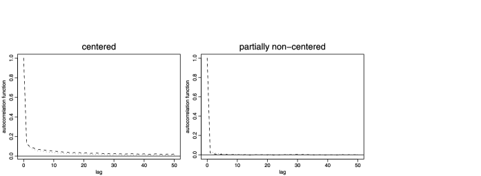
Figure 4: Autocorrelation functions for $\theta_{1}$ series (dotted) and $\theta_{2}$ series (dashed), obtained with the algorithm based on the centered parametrization (left) and with the algorithm based on the partially non-centered parametrization (right).

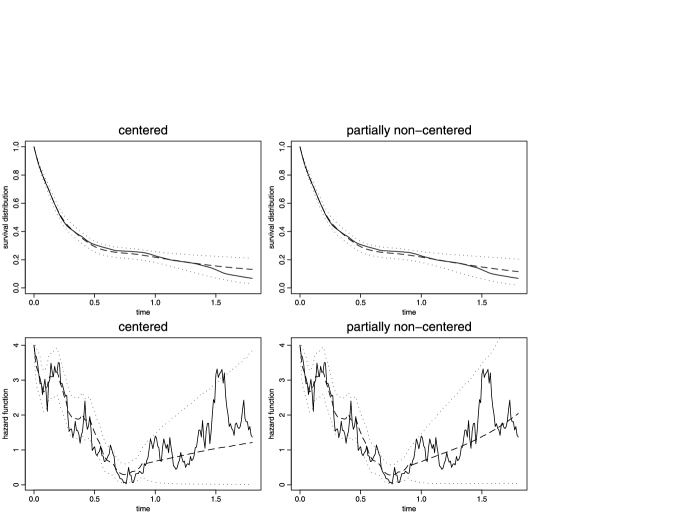
Figure 5: Top: true survival distribution distribution $1-F_{x^{\prime},x^{\prime 2}}$ (solid), together with its posterior mean (dashed) and pointwise approximate $90\%$ highest posterior bands (dotted), obtained with the algorithm based on the centered parametrization (left) and with the algorithm based on the partially non-centered parametrization (right). Bottom: true hazard function $x^{\prime 2}$ (solid), together with its posterior mean (dashed) and pointwise approximate $90\%$ highest posterior bands (dotted), obtained with the algorithm based on the centered parametrization (left) and with the algorithm based on the partially non-centered parametrization (right).

As we shall see in Section 6, another reparametrization of the model, one that turns out to be useful in the presence of covariates, is the fully non-centered parametrization in terms of $(\Theta,B)$. The diffusion $X$ can be reconstructed as a function of $\Theta$ and $B$, simply by the SDE

$$\mathrm{d}X_{t}=\beta(X_{t},\Theta)\,\mathrm{d}t+\sigma\,\mathrm{d}B_{t},\qquad t\geq 0,\qquad X_{0}=x_{0}.$$

The joint posterior distribution of $\Theta$ and $B$ has density, with respect to the product measure $\mathcal{L}^{d}\otimes\mathbb{W}_{\sigma}$, given by

$$\pi(\theta,b|y_{1},\ldots,y_{n})=Cp_{\Theta}(\theta)l\bigl{(}y_{1},\ldots,y_{n}|\theta,b_{[0,y_{[n]}]}\bigr{)},$$ (15)

where $C$ is a normalizing constant and $l(y_{1},\ldots,y_{n}|\theta,b_{[0,y_{[n]}]})=l(y_{1},\ldots,y_{n}|x_{[0,y_{[n]}]})$ is as in (4). Note that, similarly to what has been observed for the partially non-centered parametrization, (15) also characterizes the posterior distribution of the diffusion $X$ over the whole positive half-line. Moreover, the Gibbs sampler that simulates from (15) is also completely robust with respect to the choice of the time horizon $T$. In the first step, we simulate $\Theta$ conditionally on $B_{[0,y_{[n]}]}$ and the observations. Note, in particular, that the conditional distribution of $\Theta$, given $B_{[0,T]}$ and the observations, now has density, with respect to $\mathcal{L}^{d}$, proportional to $p_{\Theta}(\theta)l(y_{1},\ldots,y_{n}|\theta,b_{[0,y_{[n]}]})$. In the second step, we simulate $B$ over the time interval of interest, $[0,T]$, conditionally on $\Theta$ and the observations. For proposal distribution, we use a Brownian motion starting at $0$ and we employ the updating strategy based on overlapping Brownian bridges. In this case, when updating the Brownian motion path $b$ over the subinterval $[t_{i},t_{i+2}]$, we need to reconstruct the corresponding diffusion path $x$ over the subinterval $[t_{i},T]$ in order to preserve the continuity of the diffusion path at time $t_{i+2}$. Details are omitted.

5 Latent diffusion models for multiple groups of observations

We now discuss a straightforward generalization of the framework developed in the previous sections and deal with the case of multiple groups of observations, where the observations within each group are taken under homogeneous conditions. Consider, for example, the case in which different treatments are being administered to different groups of patients in a clinical trial.

Given $\Theta=\theta$, let $X^{[1]},\ldots,X^{[q]}$ be $q$ stochastically independent diffusion processes satisfying (2) and $F_{X^{[1]},h},\ldots,F_{X^{[q]},h}$ the relative random distributions, as in (3). Now, consider $q$ sequences of observations $(Y_{n}^{[1]})_{n},\ldots,(Y_{n}^{[q]})_{n}$ such that the random variables in $((Y_{n}^{[1]})_{n},\ldots,(Y_{n}^{[q]})_{n})$ are conditionally independent, given $F_{X^{[1]},h},\ldots,F_{X^{[q]},h}$, and the random variables in $(Y_{n}^{[k]})_{n}$ have common distribution $F_{X^{[k]},h}$ for $k=1,\ldots,q$.

The joint distribution of $Y_{1}^{[1]},\ldots,Y_{n_{1}}^{[1]},\ldots,$ $Y_{1}^{[q]},\ldots,Y_{n_{q}}^{[q]}$, given $X^{[1]}=x^{[1]},\ldots,$ $X^{[q]}=x^{[q]}$, has density, with respect to $\mathcal{L}^{n}$ (where $n=n_{1}+\cdots+n_{q}$), given by

$$l\bigl{(}y_{1}^{[1]},\ldots,y_{n_{1}}^{[1]};\ldots;y_{1}^{[q]},\ldots,y_{n_{q}}^{[q]}\big{|}x_{[0,y_{[n_{1}]}]}^{[1]},\ldots,x_{[0,y_{[n_{q}]}]}^{[q]}\bigr{)}=\prod_{k=1}^{q}l\bigl{(}y_{1}^{[k]},\ldots,y_{n_{k}}^{[k]}\big{|}x_{[0,y_{[n_{k}]}]}^{[k]}\bigr{)},$$

where $y_{[n_{k}]}:=\max\{y_{1}^{[k]},\ldots,y_{n_{k}}^{[k]}\}$ and $l(y_{1}^{[k]},\ldots,y_{n_{k}}^{[k]}|x_{[0,y_{[n_{k}]}]}^{[k]})$ is as in (4). Using the partially non-centered parametrization described in Section 4, the joint posterior distribution of $\Theta$ and $\widetilde{X}^{[1]},\ldots,\widetilde{X}^{[q]}$ has density, with respect to the product measure $\mathcal{L}^{d}\otimes\mathbb{W}_{\sigma}^{q}$, given by

$$\pi\bigl{(}\theta,\tilde{x}^{[1]},\ldots,\tilde{x}^{[q]}\big{|}y_{1}^{[1]},\ldots,y_{n_{1}}^{[1]};\ldots;y_{1}^{[q]},\ldots,y_{n_{q}}^{[q]}\bigr{)}$$

(16)

$$\quad=Cp_{\Theta}(\theta)\Biggl{[}\prod_{k=1}^{q}g\bigl{(}x_{[0,y_{[n_{k}]}]}^{[k]}|\theta\bigr{)}l\bigl{(}y_{1}^{[k]},\ldots,y_{n_{k}}^{[k]}\big{|}x_{[0,y_{[n_{k}]}]}^{[k]}\bigr{)}\Biggr{]},$$

where $C$ is a normalizing constant and $g(x_{[0,y_{[n_{k}]}]}^{[k]}|\theta)=\frac{\mathrm{d}\mathbb{P}_{y_{[n_{k}]},\theta}}{\mathrm{d}\mathbb{W}_{y_{[n_{k}]},\sigma}}(x_{[0,y_{[n_{k}]}]}^{[k]})$ is given by Girsanov’s formula (2).

The contributions of the $q$ groups of observations factorize in (5) and a simple modification of the MCMC algorithm presented in the previous sections may be used to deal with this case. Let $T_{1},\ldots,T_{q}$ be the time horizons of interest for the $q$ groups, with $T_{k}\geq y_{[n_{k}]}$ for $k=1,\ldots,q$. The Hastings-within-Gibbs algorithm for sampling from (5) alternates between

1. [1.]

2. simulation of $\Theta$, conditional on the current paths of $\widetilde{X}_{[0,y_{[n_{1}]}]}^{[1]},\ldots,$ $\widetilde{X}_{[0,y_{[n_{q}]}]}^{[q]}$;

3. for each $k$ in $\{1,\ldots,q\}$, simulation of $\widetilde{X}_{[0,T_{k}]}^{[k]}$, conditional on the observations $Y_{1}^{[k]},\ldots,Y_{n_{k}}^{[k]}$ and the current value of $\Theta$.

Consider, for example, a latent diffusion model with $q$ stochastically independent diffusion processes, $X^{[1]},\ldots,X^{[q]}$, satisfying the SDE (10). Choose the same multivariate Gaussian prior for $\Theta$ that was used in Section 3.1. Then, the distribution of $\Theta$, given $\widetilde{X}_{[0,y_{[n_{1}]}]}^{[1]}=x_{[0,y_{[n_{1}]}]}^{[1]},\ldots,$ $\widetilde{X}_{[0,y_{[n_{q}]}]}^{[q]}=x_{[0,y_{[n_{q}]}]}^{[q]}$, is still Gaussian, with mean vector and covariance matrix as in (11), but with

$$S_{i} := \frac{1}{\sigma^{2}}\Biggl{[}\sum_{k=1}^{q}\int_{0}^{y_{[n_{k}]}}f_{i}\bigl{(}x^{[k]}_{t}\bigr{)}\,\mathrm{d}x^{[k]}_{t}\Biggr{]}+\sum_{j=1}^{d}\lambda_{ij}\mu_{j},$$

$$L_{ij} := \frac{1}{\sigma^{2}}\Biggl{[}\sum_{k=1}^{q}\int_{0}^{y_{[n_{k}]}}f_{i}\bigl{(}x^{[k]}_{t}\bigr{)}f_{j}\bigl{(}x^{[k]}_{t}\bigr{)}\,\mathrm{d}t\Biggr{]}+\lambda_{ij}$$

for $i=1,\ldots,d$, $j=1,\ldots,d$. The update of the parameter $\Theta$ can thus be performed by sampling directly from this conditional distribution. The second step may be carried out by $q$ repetitions of the updating mechanism described in Sections 3.1 and 4.

Note that we are here considering a simple hierarchical structure, where inference on the separate groups is linked only at the level of the finite-dimensional parameter $\Theta$. For some applications, this might allow too little borrowing of strength for inference across groups of patients. In Section 6, we shall instead describe a more complex hierarchical structure, suitable in the presence of covariates and allowing for a much stronger borrowing of strength for inference across individuals.

5.1 An illustrative application to a real data set with multiple groups of observations

In this section, we show the implementation of the latent diffusion model for multiple groups of observations via an illustrative application to a small data set from a clinical trial, one that has been considered in a number of papers in the context of survival analysis, among them Gehan (1965), Cox (1972), Wei (1984) and Xu and O’Quigley (2000) in the non-Bayesian literature and Kalbfleisch (1978), Laud, Damien and Smith (1998) and Damien and Walker (2002) in the Bayesian literature. In the trial, reported by Freireich (1963), 6-mercaptopurine (6-MP) was compared to a placebo in the maintenance of remission in acute leukemia. The following lengths of remission in weeks were recorded for 42 patients, half of which treated with the 6-MP drug and half with the placebo (a $+$ sign indicates a censored observation):

1. [placebo:]

2. 6, 6, 6, 6$+$, 7, 9$+$, 10, 10$+$, 11$+$, 13, 16, 17$+$, 19$+$, 20$+$, 22, 23, 25$+$, 32$+$, 32$+$, 34$+$, 35$+$,

3. $1,1,2,2,3,4,4,5,5,8,8,8,8,11,11,12,12,15,17,22,23.$

We thus consider a model for two groups of observations, namely the 6-MP drug group and the placebo group. As latent diffusion model, we shall use the stochastic perturbation around the Weibull described in Section 2.1. Recall that this model has base diffusion satisfying the SDE

$$\mathrm{d}X_{t}=\theta_{1}(\operatorname{sign}(X_{t}))|X_{t}|^{\theta_{2}}\,\mathrm{d}t+\sigma\,\mathrm{d}B_{t},\qquad t\geq 0,\qquad X_{0}=x_{0}>0,$$

and hazard function $h(u)=|u|$.

We express the data as fractions of one year and choose as time horizons of interest $T_{1}=T_{2}=0.75$, corresponding to 9 months (39 weeks). We take $\Theta_{1}$ and $\Theta_{2}$ to be a priori independent, with a Gaussian prior distribution for $\Theta_{1}$, mean $\mu=0$, variance $1/\lambda=5$, and a uniform prior over $[0,1]$ for $\Theta_{2}$. Moreover, we set $x_{0}=0.8$ and $\sigma=8$. We then run the Hastings-within-Gibbs algorithm based on the partially non-centered parametrization. The update of $\Theta_{1}$ is performed by sampling directly from the conditional distribution $\Theta_{1}$, given $\Theta_{2},\widetilde{X}_{[0,y_{[n_{1}]}]}^{[1]},\widetilde{X}_{[0,y_{[n_{2}]}]}^{[2]}$, which is still Gaussian with mean $\frac{S+\lambda\mu}{L+\lambda}$ and variance $\frac{1}{L+\lambda}$, where

$$S:=\frac{1}{\sigma^{2}}\Biggl{[}\sum_{j=1}^{2}\int_{0}^{y_{[n_{j}]}}\bigl{(}\bigl{(}\operatorname{sign}\bigl{(}x^{[j]}_{t}\bigr{)}\bigr{)}\bigl{|}x^{[j]}_{t}\bigr{|}^{\theta_{2}}\bigr{)}\,\mathrm{d}x^{[j]}_{t}\Biggr{]}\quad\mbox{and}\quad L:=\frac{1}{\sigma^{2}}\Biggl{[}\sum_{j=1}^{2}\int_{0}^{y_{[n_{j}]}}\bigl{(}\bigl{|}x^{[j]}_{t}\bigr{|}^{\theta_{2}}\bigr{)}^{2}\,\mathrm{d}t\Biggr{]}.$$

For the update of $\Theta_{2}$, we use an independence sampler with a Beta proposal distribution, with parameters $(1/2,1/2)$. The update of $\widetilde{X}^{[1]}$ and $\widetilde{X}^{[2]}$ is carried out as described in the previous sections. The algorithm is run for 200 000 iterations and the first 2000 are discarded as burn-in.

Figure 6 displays the MCMC estimates of the survival distributions of the two groups, 6-MP drug and placebo, together with the relative Kaplan–Meier curves. Note that the MCMC estimates of the two survival distributions are closer to one another than the two Kaplan–Meier curves, thus indicating borrowing of strength for inference among the two groups. Hence, the latent diffusion model, which gains much flexibility over a fully parametric model by introducing randomness around it, does not suffer from the opposite problem of being too data-driven. Figure 6 also displays the MCMC estimates of the hazards of the two groups.

We could now verify the efficacy of 6-MP drug treatment as proposed in Damien and Walker (2002). In particular, under the hypothesis that the 6-MP drug is inefficient, we would regard all patients as belonging to a single group, instead of two. We could then implement the latent diffusion model based on the stochastic perturbation of the Weibull, but with just one diffusion process. Let M₁ denote the model where all patients belong to a single group (corresponding to the hypothesis $H_{1}$ of null efficacy of the 6-MP drug) and let M₂ denote the model considered above (corresponding to the hypothesis $H_{2}$ of efficacy of the 6-MP drug). If the a priori probabilities of hypotheses $H_{1}$ and $H_{2}$ are set equal to 0.5, the Bayes factor

$$\mbox{BF}=\frac{\mbox{probability density of data under model M${}_{1}$}}{\mbox{probability density of data under model M${}_{2}$}}$$

gives the posterior odds in favor of $H_{1}$. As expected, the computed Bayes factor ($\mathrm{BF}=9\times 10^{-6}$) provides strong evidence for the efficacy of the 6-MP drug.

Figure 6: Left: posterior mean survival distributions and pointwise approximate $90\%$ highest posterior bands for the group of patients treated with 6-MP drug (solid) and for the group of patients treated with the placebo (dashed), together with corresponding Kaplan–Meier curves. Right: posterior mean hazards for the group of patients treated with 6-MP drug (solid) and for the group of patients treated with the placebo (dashed).

6 Latent diffusion models with covariates

Covariates can be included in the latent diffusion models described in a very natural way, as directly influencing the underlying diffusion. For instance, if $\mathbf{Z}$ is a vector of $p$ covariates measured at time 0, we can use the model based on the diffusion satisfying the SDE

$$\mathrm{d}X_{t} = \beta(X_{t},\mathbf{z},\theta)\,\mathrm{d}t+\sigma\,\mathrm{d}B_{t},\qquad t\geq 0,$$

$$X_{0} = x_{0}(\mathbf{z},\theta).$$

In particular, following suggestions of Aalen and Gjessing (2001) andAalen, Borgan and Gjessing (2008) for barrier hitting models, those covariates which represent measures of how far the underlying process that leads to the event has advanced (such as staging measures in cancer) may be taken to influence the starting point of the diffusion. Those covariates which instead represent causal influence on the development of the process may be taken to influence the drift of the diffusion.

Let $\mathbf{z}$ take values $\mathbf{z}^{[1]},\ldots,\mathbf{z}^{[q]}$. Then, (6) gives $q$ different diffusions, $X^{{[\mathbf{z}=\mathbf{z}^{[1]}}]},\ldots,X^{{[\mathbf{z}=\mathbf{z}^{[q]}}]}$, driven by the same Brownian motion $B$, with

$$\mathrm{d}X_{t}^{{[\mathbf{z}=\mathbf{z}^{[k]}}]} = \beta\bigl{(}X_{t}^{{[\mathbf{z}=\mathbf{z}^{[k]}}]},\mathbf{z}^{[k]},\theta\bigr{)}\,\mathrm{d}t+\sigma\,\mathrm{d}B_{t},\qquad t\geq 0,$$

$$X_{0} = x_{0}\bigl{(}\mathbf{z}^{[k]}\bigr{)}$$

for $k=1,\ldots,q$. Denote by $F_{X^{{[\mathbf{z}=\mathbf{z}^{[1]}}]},h},\ldots,F_{X^{{[\mathbf{z}=\mathbf{z}^{[q]}}]},h}$ the relative random distributions, as in (3). Moreover, denote by $Y_{1}^{{[\mathbf{z}=\mathbf{z}^{[k]}}]},\ldots,Y_{n_{k}}^{{[\mathbf{z}=\mathbf{z}^{[k]}}]}$ the survival times of the $n_{k}$ individuals having covariates $\mathbf{z}=\mathbf{z}^{[k]}$ for $k=1,\ldots,q$. The survival times $Y_{1}^{{[\mathbf{z}=\mathbf{z}^{[k]}}]},\ldots,Y_{n_{k}}^{{[\mathbf{z}=\mathbf{z}^{[k]}}]}$, conditionally on $F_{X^{{[\mathbf{z}=\mathbf{z}^{[k]}}]},h}$, are i.i.d. with common distribution $F_{X^{{[\mathbf{z}=\mathbf{z}^{[k]}}]},h}$. Since the $q$ diffusions are driven by the same Brownian motion, it is here more natural to use the fully non-centered parametrization of the model, described in Section 4. In particular, the joint distribution of $Y_{1}^{{[\mathbf{z}=\mathbf{z}^{[1]}}]},\ldots,Y_{n_{1}}^{{[\mathbf{z}=\mathbf{z}^{[1]}}]},\ldots,Y_{1}^{{[\mathbf{z}=\mathbf{z}^{[q]}}]},\ldots,Y_{n_{q}}^{{[\mathbf{z}=\mathbf{z}^{[q]}}]},$ given $B=b$ and $\Theta=\theta$, has density, with respect to $\mathcal{L}^{n}$ (where $n=n_{1}+\cdots+n_{q}$), given by

$$l\bigl{(}y_{1}^{{[\mathbf{z}=\mathbf{z}^{[1]}}]},\ldots,y_{n_{1}}^{{[\mathbf{z}=\mathbf{z}^{[1]}}]};\ldots;y_{1}^{{[\mathbf{z}=\mathbf{z}^{[q]}}]},\ldots,y_{n_{q}}^{{[\mathbf{z}=\mathbf{z}^{[q]}}]}\big{|}\theta,b_{[0,y_{[n]}]},\mathbf{z}^{[1]},\ldots,\mathbf{z}^{[q]}\bigr{)}$$

$$\quad=\prod_{k=1}^{q}l\bigl{(}y_{1}^{{[\mathbf{z}=\mathbf{z}^{[k]}}]},\ldots,y_{n_{k}}^{{[\mathbf{z}=\mathbf{z}^{[k]}}]}\big{|}\theta,b_{[0,y_{[n_{k}]}]},\mathbf{z}^{[k]}\bigr{)},$$

where $y_{[n]}:=\max\{y_{1},\ldots,y_{n}\}$, $y_{[n_{k}]}:=\max\{y_{1}^{{[\mathbf{z}=\mathbf{z}^{[k]}}]},\ldots,y_{n_{k}}^{{[\mathbf{z}=\mathbf{z}^{[k]}}]}\}$ and

$$l\bigl{(}y_{1}^{{[\mathbf{z}=\mathbf{z}^{[k]}}]},\ldots,y_{n_{k}}^{{[\mathbf{z}=\mathbf{z}^{[k]}}]}\big{|}\theta,b_{[0,y_{[n_{k}]}]},\mathbf{z}^{[k]}\bigr{)}=l\bigl{(}y_{1}^{{[\mathbf{z}=\mathbf{z}^{[k]}}]},\ldots,y_{n_{k}}^{{[\mathbf{z}=\mathbf{z}^{[k]}}]}\big{|}x_{[0,y_{[n_{k}]}]}^{{[\mathbf{z}=\mathbf{z}^{[k]}}]}\bigr{)}$$

is as in (4). The joint posterior distribution of $\Theta$ and $B$ has density, with respect to the product measure $\mathcal{L}^{d}\otimes\mathbb{W}_{\sigma}$, given by

$$\pi\bigl{(}\theta,b\big{|}y_{1}^{{[\mathbf{z}=\mathbf{z}^{[1]}}]},\ldots,y_{n_{1}}^{{[\mathbf{z}=\mathbf{z}^{[1]}}]};\ldots;y_{1}^{{[\mathbf{z}=\mathbf{z}^{[q]}}]},\ldots,y_{n_{q}}^{{[\mathbf{z}=\mathbf{z}^{[q]}}]};\mathbf{z}^{[1]},\ldots,\mathbf{z}^{[q]}\bigr{)}$$

(18)

$$\quad=Cp_{\Theta}(\theta)\prod_{k=1}^{q}l\bigl{(}y_{1}^{{[\mathbf{z}=\mathbf{z}^{[k]}}]},\ldots,y_{n_{k}}^{{[\mathbf{z}=\mathbf{z}^{[k]}}]}\big{|}\theta,b_{[0,y_{[n_{k}]}]},\mathbf{z}^{[k]}\bigr{)}.$$

Note that this model is structurally different from the model for multiple groups of observations described in Section 5 since the distributions of the survival times are here linked at the level of the Brownian motion, allowing a much stronger borrowing of strength for inference across individuals who share a common value of even just one of the $p$ covariates.

As usual, we denote by $T$ the time horizon of interest, $T\geq y_{[n]}$. The Hastings-within-Gibbs algorithm for sampling from (6) alternates between

1. [1.]

2. simulation of $\Theta$, conditional on the current path of $B_{[0,y_{[n]}]}$, the observations and the covariates;

3. simulation of $B_{[0,T]}$, conditional on the current value of $\Theta$, the observations and the covariates.

In particular, the update of the Brownian motion $B_{[0,T]}$ can be carried out via the updating strategy based on overlapping Brownian bridges, as described in Section 4.

6.1 An illustrative application to a real-world data set with covariates

In this section, we illustrate how to efficiently handle the model with covariates via an application to a data set concerning 272 patients diagnosed with non-small cell lung cancer. The data set is described in detail in Muers, Shevlin and Brown (1996). Survival times are measured in months from the time of diagnosis (with 17% of censoring) and some covariates are recorded at the time of diagnosis. Just to give an illustration of the model, we shall consider here two covariates: sex ($F=0$: male and $F=1$: female) and hoarseness ($H=0$: absent and $H=1$: present). Using, for instance, the model based on the stochastic perturbation around the Weibull, we can include these covariates as follows:

$$\mathrm{d}X_{t} = \exp\{\theta_{10}+\theta_{11}F\}(\operatorname{sign}(X_{t}))|X_{t}|^{\theta_{2}}\,\mathrm{d}t+\sigma\,\mathrm{d}B_{t},\qquad t\geq 0,$$

$$X_{0} = \exp\{\theta_{00}+\theta_{01}F+\theta_{02}H\}.$$

Note that, following the suggestion of Aalen, Borgan and Gjessing (2008), we have modeled the covariate hoarseness, which only represents a measure of how far the lung tumor has advanced, as influencing the starting point of the diffusion; we have instead taken the covariate sex to influence both the starting point and the drift of the diffusion, in order to account for possible differences between males and females, both in the hazards at time of diagnosis and in the hazard dynamics. The covariate combinations determine four different diffusions, $X^{{[F=0,H=0]}}$, $X^{{[F=0,H=1]}}$, $X^{{[F=1,H=0]}}$ and $X^{{[F=1,H=1]}}$, driven by the same Brownian motion. According to this model, the hazard at time 0 (the time of diagnosis) of patients suffering from hoarseness is $\exp\{\theta_{02}\}$ times that of patients not suffering from hoarseness and the hazard at time 0 of female patients is $\exp\{\theta_{01}\}$ times that of male patients; moreover, $\exp\{\theta_{11}\}$ gives a measure of the different progression rate of the cancer in female patients with respect to male patients.

We express the data as fractions of a quadrennium and choose as time horizon $T$ the maximum of the observations, corresponding to about 37 months. In order to avoid dependencies among the $(\theta_{00},\theta_{01},\theta_{02})$ parameters and among the $(\theta_{10},\theta_{11})$ parameters, we reparametrize them in terms of $(\eta_{00},\theta_{01},\theta_{02})$ and $(\eta_{10},\theta_{11})$, with $\theta_{00}=\eta_{00}-p_{F}\theta_{01}-p_{H}\theta_{02}$ and $\theta_{10}=\eta_{10}-p_{F}\theta_{11}$, where we have denoted by $p_{F}$ and $p_{H}$ the percentage of females patients and the percentage of patients suffering from hoarseness, respectively. We take all of the parameters to be a priori independent, with Gaussian priors with mean $0$ and variance $5$ for all parameters except $\Theta_{2}$, for which we use a uniform prior over $[0,1]$. Moreover, we set $\sigma=8$. We then run the Hastings-within-Gibbs algorithm based on the non-centered parametrization of the model. The update of the parameters is performed via independence samplers having proposal distributions equal to the priors. The algorithm is run for 200 000 iterations and the first 2000 are discarded as burn-in.

Figure 7 shows posterior mean survival distributions, together with Kaplan–Meier curves, for male patients without hoarseness at time of diagnosis ($F=0,H=0$, solid line), for male patients with hoarseness ($F=0,H=1$, dotted and dashed line), for female patients without hoarseness ($F=1,H=0$, dashed line) and for female patients with hoarseness ($F=1,H=1$, dotted line). The four survivals are also plotted separately in Figure 8 with $90\%$ highest posterior bands. Figure 7 also displays the posterior mean hazard functions for the four covariate combinations. In particular, the posterior mean hazard at time 0 of patients suffering from hoarseness is 2.2 times bigger than that of patients not suffering from hoarseness, whereas the hazard at time 0 of female patients is 0.6 times that of male patients.

Note that even though we have only considered categorical covariates in this illustrative application, quantitative covariates can also be included in the model; however, it may be necessary to categorize these covariates in order to have a sufficient number of observations for each of the diffusion processes. This, of course, requires larger data sets.

Figure 7: Left: posterior mean survival distributions, together with Kaplan–Meier curves, for male patients without hoarseness at time of diagnosis ($F=0,H=0$, solid line), for male patients with hoarseness ($F=0,H=1$, dotted and dashed line), for female patients without hoarseness ($F=1,H=0$, dashed line) and for female patients with hoarseness ($F=1,H=1$, dotted line). Right: the same for posterior mean hazard functions.

Figure 8: Upper-left: posterior mean survival distribution and pointwise approximate $90\%$ highest posterior bands, together with Kaplan–Meier curve, for male patients without hoarseness. Upper-right: the same for male patients with hoarseness. Lower-left: the same for female patients without hoarseness. Lower-right: the same for female patients with hoarseness.

7 Generalization to the case of unknown diffusion coefficient

An important generalization of the models we have considered thus far consists of considering diffusion processes with unknown diffusion coefficient $\sigma$ since $\sigma$ describes a natural measure of prior uncertainty. We briefly discuss how to deal with this case.

Let $\Sigma$ be a real random variable. Given $\Theta=\theta$ and $\Sigma=\sigma$, consider the scalar diffusion process $X$ solution of the SDE (2) and denote by $\mathbb{P}_{T,\theta,\sigma}$ the law of $X_{[0,T]}$. Let $p_{\Sigma}(\cdot)$ be the prior density, with respect to $\mathcal{L}$, of $\Sigma$ (for simplicity, we take $\Theta$ and $\Sigma$ to be stochastically independent a priori). Let us consider, for instance, the centered parametrization of the model. The joint posterior distribution of $(\Theta,\Sigma,X_{[0,T]})$ has density, with respect to $\mathcal{L}^{d+1}\otimes\mathbb{W}_{T,\sigma}$, given by

$$\pi\bigl{(}\theta,\sigma,x_{[0,T]}|y_{1},\ldots,y_{n}\bigr{)}=Cp_{\Theta}(\theta)p_{\Sigma}(\sigma)g\bigl{(}x_{[0,T]}|\theta,\sigma\bigr{)}l\bigl{(}y_{1},\ldots,y_{n}|x_{[0,y_{[n]}]}\bigr{)},$$ (19)

where $C$ is a normalizing constant and $g(x_{[0,T]}|\theta,\sigma):=\frac{\mathrm{d}\mathbb{P}_{T,\theta,\sigma}}{\mathrm{d}\mathbb{W}_{T,\sigma}}(x_{[0,T]})$ is given by Girsanov’s formula (2).

The quadratic variation of a diffusion processes, having diffusion coefficient $\sigma$, satisfies

$$\lim_{m\to\infty}\sum_{i=1}^{m}\bigl{(}X_{ti/m}-X_{t(i-1)/m}\bigr{)}^{2}=t\sigma^{2},\qquad\mathbb{W}_{T,\sigma}\mbox{-a.s. for all }t.$$

Therefore, the conditional distribution of $\Sigma$, given the diffusion $X_{[0,T]}$, degenerates to a point mass and $\Sigma$ is completely determined by the diffusion path. In practice, we cannot simulate the diffusion path in continuous time, but just at discrete time instants. In any case, the finer the discrete-time approximation $\{X_{iT/m}\colon\ i=1,\ldots,m\}$ of the diffusion $X_{[0,T]}$, the stronger the dependence between $\{X_{iT/m}\colon\ i=1,\ldots,m\}$ and $\Sigma$. Consider the algorithm for the simulation from (19) that alternates between:

1. [1.]

2. simulation of $\Theta$, conditional on the current value of $\Sigma$ and the current path of $X_{[0,T]}$;

3. simulation of $\Sigma$, conditional on the current value of $\Theta$ and the current path of $X_{[0,T]}$;

4. simulation of $X_{[0,T]}$, conditional on the observations and the current values of $\Theta$ and $\Sigma$.

The finer the approximation of the diffusion path, the worse the convergence of the algorithm becomes. In the limiting case $m=\infty$ (i.e., if the diffusion process could be simulated in continuous time), this scheme would be reducible; see Roberts and Stramer (2001). An alternative way to see this problem is to note that the collection of measures $\{\mathbb{W}_{T,\sigma}\colon\ \sigma\in\mathbb{R}\}$ are mutually singular and, therefore, so are the measures $\{\mathbb{P}_{T,\theta,\sigma}\colon\ \sigma\in\mathbb{R}\}$.

In this case, the need for a different parametrization of the model is thus compelling. Following Roberts and Stramer (2001), we parametrize the model in terms of $(\Theta,\Sigma,\dot{X})$, where $\dot{X}_{t}=(X_{t}-X_{0})/\Sigma$. By Itô’s formula,

$$\mathrm{d}\dot{X}_{t}=\frac{\beta(\dot{X}_{t},\Theta)}{\Sigma}\,\mathrm{d}t+\mathrm{d}B_{t},\qquad t\geq 0,\qquad\dot{X}_{0}=0.$$

The distribution of $\dot{X}_{[0,T]}$ depends on $\Sigma$, but any realization of $\dot{X}_{[0,T]}$ contains only finite information about $\Sigma$. Analogous reparametrizations are derived starting from the ones described in Section 4. MCMC algorithms based on these reparametrizations can be obtained as simple modifications of the ones previously described.

Consider the toy example described in Section 3.2 and assume the same model, but let the diffusion process have an unknown diffusion coefficient. Let the prior for this coefficient be exponential with mean 1. Figure 9 displays the results obtained with the MCMC algorithm based on the reparametrization $(\Theta,\Sigma,\dot{X})$. Specifications of the algorithm are as in Section 3.2. Note that the mixing for $\sigma$ is slow relative to the very good mixing for $\theta_{1}$ and $\theta_{2}$, but this does not prevent good estimates of the survival distribution, density and hazard being obtained. Slow mixing for $\sigma$ could probably be improved by a further reparametrization of the model.

Figure 9: This corresponds to Figure 2, but for the model with unknown diffusion coefficient. The lower-right plot also displays the autocorrelation function for $\sigma$ series (dotted-dashed line).

Alternatively to the case of an unknown diffusion coefficient, it would be possible to consider models based on diffusion processes having $\sigma=1$, but with hazard function $h(\Gamma,X)$, where $\Gamma$ is a random parameter. A reparametrization of the model would also be necessary in this case.

8 Discussion

In this paper, we have described latent diffusion models for survival analysis and have shown that these models can be efficiently treated by means of MCMC techniques. We have dealt with the case of multiple groups of observations, typical of clinical trials, and we have shown how covariates can be efficiently included in the models. We have outlined how, in the described framework, it is possible to consider stochastic perturbations of common survival models. In particular, we have used a stochastic perturbation of the Weibull model in some illustrative applications to small data sets, with multiple groups of observations and with covariates. Applications to larger data sets, where the potential of a latent diffusion model may be fully expressed, will be the object of future work. All analyses presented are computationally feasible within R (see R Development Core Team (2007)).

Another generalization of the model we intend to explore regards random probabilities based on jump diffusion processes. As observed in Section 2, the cumulative hazard functions associated with random probabilities based on diffusions are smooth, being the integrals of continuous processes. By replacing the diffusion process with a jump diffusion process, it would be possible to capture sudden changes in the behavior of cumulative hazards that might be due to some kind of shock experienced by the population. Hazards modeled through stochastic processes with jumps have been studied, for instance, by Gjessing, Aalen and Hjort (2003).

References

- Aalen, Borgan and Gjessing (2008) Aalen, O.O., Borgan, Ø. and Gjessing, H.K. (2008). Survival and Event History Analysis. A Process Point of View. New York: Springer. MR2449233
- Aalen and Gjessing (2001) Aalen, O.O. and Gjessing, H.K. (2001). Understanding the shape of the hazard rate: A process point of view (with discussion). Statist. Sci. 16 1–22. MR1838599
- Aalen and Gjessing (2004) Aalen, O.O. and Gjessing, H.K. (2004). Survival models based on the Ornstein–Uhlenbeck process. Lifetime Data Anal. 10 407–423. MR2125423
- Beskos et al. (2006) Beskos, A., Papaspiliopoulos, O., Roberts, G.O. and Fearnhead, P. (2006). Exact and computationally efficient likelihood-based estimation for discretely observed diffusion processes. J. R. Stat. Soc. Ser. B Stat. Methodol. 68 333–382. MR2278331
- Cox (1972) Cox, D.R. (1972). Regression models and life-tables (with discussion). J. R. Stat. Soc. Ser. B Stat. Methodol. 34 187–220. MR0341758
- Damien and Walker (2002) Damien, P. and Walker, S. (2002). A Bayesian non-parametric comparison of two treatments. Scand. J. Statist. 29 51–56. MR1894380
- Doksum (1974) Doksum, K. (1974). Tailfree and neutral random probabilities and their posterior distributions. Ann. Probab. 2 183–201. MR0373081
- Dykstra and Laud (1981) Dykstra, R.L. and Laud, P. (1981). A Bayesian nonparametric approach to reliability. Ann. Statist. 9 356–367. MR0606619
- Elerian, Chib and Shephard (2001) Elerian, O., Chib, S. and Shephard, N. (2001). Likelihood inference for discretely observed nonlinear diffusions. Econometrica 69 959–993. MR1839375
- Ferguson (1974) Ferguson, T.S. (1974). Prior distributions on spaces of probability measures. Ann. Statist. 2 615–629. MR0438568
- Ferguson and Phadia (1979) Ferguson, T.S. and Phadia, E.G. (1979). Bayesian nonparametric estimation based on censored data. Ann. Statist. 7 163–186. MR0515691
- Freireich (1963) Freireich, E.O. (1963). The effect of 6 mercaptopurine on the duration of steroid induced remission in acute leukemia. Blood 21 699–716.
- Gehan (1965) Gehan, E.A. (1965). A generalized Wilcoxon test for comparing arbitrarily singly-censored samples. Biometrika 52 203–223. MR0207130
- Gelfand, Sahu and Carlin (1995) Gelfand, A.E., Sahu, S.K. and Carlin, B.P. (1995). Efficient parameterisations for normal linear mixed models. Biometrika 82 479–488. MR1366275
- Gelfand, Sahu and Carlin (1996) Gelfand, A.E., Sahu, S.K. and Carlin, B.P. (1996). Efficient parametrizations for generalized linear mixed models. In Bayesian Statistics 5 165–180. New York: Oxford Univ. Press. MR1425405
- Gjessing, Aalen and Hjort (2003) Gjessing, H.K., Aalen, O.O. and Hjort, N.L. (2003). Frailty models based on Lévy processes. Adv. in Appl. Probab. 35 532–550. MR1970486
- Hills and Smith (1992) Hills, S.E. and Smith, A.F.M. (1992). Parameterization issues in Bayesian inference. In Bayesian Statistics 4 227–246. New York: Oxford Univ. Press. MR1380279
- Hjort (1990) Hjort, N.L. (1990). Nonparametric Bayes estimators based on beta processes in models for life history data. Ann. Statist. 18 1259–1294. MR1062708
- Ishwaran and James (2004) Ishwaran, H. and James, L.F. (2004). Computational methods for multiplicative intensity models using weighted gamma processes: Proportional hazards, marked point processes and panel count data. J. Amer. Statist. Assoc. 99 175–190. MR2054297
- Kalbfleisch (1978) Kalbfleisch, J.D. (1978). Non-parametric Bayesian analysis of survival time data. J. R. Stat. Soc. Ser. B Stat. Methodol. 40 214–221. MR0517442
- Kloeden and Platen (1992) Kloeden, P.E. and Platen, E. (1992). Numerical solution of stochastic differential equations. In Applications of Mathematics 23. Berlin: Springer-Verlag. MR1214374
- Laud, Damien and Smith (1998) Laud, P.W., Damien, P. and Smith, A.F.M. (1998). Bayesian nonparametric and covariate analysis of failure time data. In Practical Nonparametric and Semiparametric Bayesian Statistics. Lecture Notes in Statist. 133 213–225. New York: Springer. MR1630083
- Lo and Weng (1989) Lo, A.Y. and Weng, C.-S. (1989). On a class of Bayesian nonparametric estimates. II. Hazard rate estimates. Ann. Inst. Statist. Math. 41 227–245. MR1006487
- Muers, Shevlin and Brown (1996) Muers, M.F., Shevlin, P. and Brown, J. (1996). Prognosis in lung cancer: Physicians’s opinions compared with outcome and a predictive model. Thorax 51 894–902.
- Myers (1981) Myers, L.E. (1981). Survival functions induced by stochastic covariate processes. J. Appl. Probab. 18 523–529. MR0611796
- Papaspiliopoulos, Roberts and Sköld (2003) Papaspiliopoulos, O., Roberts, G.O. and Sköld, M. (2003). Non-centered parameterizations for hierarchical models and data augmentation (with discussion). In Bayesian Statistics 7 307–326. New York: Oxford Univ. Press. MR2003180
- Papaspiliopoulos, Roberts and Sköld (2007) Papaspiliopoulos, O., Roberts, G.O. and Sköld, M. (2007). A general framework for the parametrization of Hierarchical models. Statist. Sci. 22 59–73. MR2408661
- R Development Core Team (2007) R Development Core Team (2007). R: A Language and Environment for Statistical Computing. Vienna, Austria: R Foundation for Statistical Computing. ISBN 3-900051-07-0.
- Roberts and Stramer (2001) Roberts, G.O. and Stramer, O. (2001). On inference for partially observed nonlinear diffusion models using the Metropolis–Hastings algorithm. Biometrika 88 603–621. MR1859397
- Rogers and Williams (2000) Rogers, L.C.G. and Williams, D. (2000). Diffusions, Markov Processes, and Martingales, Volume 2: Itô Calculus. Cambridge Mathematical Library, Cambridge: Cambridge Univ. Press.
- Shephard and Pitt (1997) Shephard, N. and Pitt, M.K. (1997). Likelihood analysis of non-Gaussian measurement time series. Biometrika 84 653–667. MR1603940
- Stroock and Varadhan (2006) Stroock, D.W. and Varadhan, S.R.S. (2006). Multidimensional Diffusion Processes. Berlin: Springer-Verlag. MR2190038
- Susarla and Van Ryzin (1976) Susarla, V. and Van Ryzin, J. (1976). Nonparametric Bayesian estimation of survival curves from incomplete observations. J. Amer. Statist. Assoc. 71 897–902. MR0436445
- Wei (1984) Wei, L.J. (1984). Testing goodness of fit for proportional hazards model with censored observations. J. Amer. Statist. Assoc. 79 649–652. MR0763583
- Woodbury and Manton (1977) Woodbury, M.A. and Manton, K.G. (1977). A random-walk model of human mortality and aging. Theoret. Population Biology 11 37–48. MR0490068
- Xu and O’Quigley (2000) Xu, R. and O’Quigley, J. (2000). Proportional hazards estimate of the conditional survival function. J. R. Stat. Soc. Ser. B Stat. Methodol. 62 667–680. MR1796284
- Yashin (1985) Yashin, A.I. (1985). Dynamics of survival analysis: Conditional Gaussian property versus the Cameron–Martin formula. In Statistics and Control of Stochastic Processes 466–485. New York: Optimization Software. MR0808217
- Yashin and Vaupel (1986) Yashin, A.I. and Vaupel, J.W. (1986). Measurement and estimation in heterogeneous populations. In Immunology and Epidemiology. Lecture Notes in Biomath. 65 198–206. Berlin: Springer. MR0849172