GEANT4 Simulations of Gamma-Ray Emission from Accelerated Particles in Solar Flares

Abstract

Gamma-ray spectroscopy provides diagnostics of particle acceleration in solar flares, but care must be taken when interpreting the spectra due to effects of the angular distribution of the accelerated particles (such as relativistic beaming) and Compton reprocessing of the radiation in the solar atmosphere. In this paper, we use the GEANT4 Monte Carlo package to simulate the interactions of accelerated electrons and protons and study these effects on the gamma-rays resulting from electron bremsstrahlung and pion decay. We consider the ratio of the 511 keV annihilation-line flux to the continuum at 200 keV and in the energy band just above the nuclear de-excitation lines (8–15 MeV) as a diagnostic of the accelerated particles and a point of comparison with data from the X17 flare of 2003 October 28. We also find that pion secondaries from accelerated protons produce a positron annihilation line component at a depth of $\sim$ 10 g cm^-2, and that the subsequent Compton scattering of the 511 keV photons produces a continuum that can mimic the spectrum expected from the 3$\gamma$ decay of orthopositronium.

1. Introduction

In solar flares, electrons and ions are accelerated to non-thermal energies. When these particles interact with the ambient medium, they can produce photons with energies up to the gamma-ray range. The electrons produce continuum emission via the bremsstrahlung process, while the ions (protons and heavier nuclei) can produce excited and radioactive nuclei which, through de-excitation or decay, make emission lines usually $\lesssim$ 7 MeV. Ions with energy above $\sim$ 200 MeV can produce pions by interacting with ambient nuclei. These pions then produce gamma-ray continuum via $\pi^{0}\rightarrow 2\gamma$ or $\pi^{\pm}\rightarrow\mu^{\pm}\rightarrow e^{\pm}\rightarrow\gamma_{brem}$. There is also 511 keV line emission from annihilation of positrons created by the decay of $\beta^{+}$-emitting radioactive nuclei or $\pi^{+}$. Whether radioactive nuclei or $\pi^{+}$ contribute more to the positron population depends on the hardness of the injected ions (Murphy & Ramaty, 1984). Positrons may also come from the $e^{-}e^{+}$ pair production process of the gamma-ray continuum.

These continua and lines provide information on particle acceleration in solar flares, but we can only observe those photons that reach us. Since the accelerated electrons are relativistic, the angular distribution of bremsstrahlung will tend to follow that of the original electrons, so electrons beamed downward along the magnetic field will put most of their radiation into the Sun. Photons created deep in the solar atmosphere by any process are less likely to escape than those created in the corona or chromosphere. These effects will change the relative luminosity of different spectral components, but the location and directionality of the photon production processes will also change the spectral shape of each as well. Bremsstrahlung intrinsically creates different spectra in different directions, with the hardest spectrum in the beam direction. Compton scattering can also affect the observed spectra (Kotoku et al., 2007, e.g.) by scattering photons to lower energy. The importance of this process depends on both the depth where the original photons are produced and their direction relative to the line of sight. Accurate simulations of the location, beaming, reprocessing, and absorption of flare photons are therefore just as important to interpreting spectra as modeling of the original radiation mechanism.

Examples of the importance of directionality and location in interpreting observed bremsstrahlung spectra are seen in recent work by Krucker et al. (2008) and Kontar & Brown (2006). The picture of electrons accelerated directly down field lines into the deep solar atmosphere is seldom found to agree with observations. Strong scattering, as from interactions with magnetohydrodynamic waves, can make the distribution function evolve into one that is more isotropic than when the electrons were injected into the magnetic loop. Bret (2009) compared different kinds of instabilities that may cause this anisotropy decrease. The evolution speed of the distribution function is sensitive to the loop magnetic field as described by Karlicky & Kasparova (2009). Magnetic mirroring can produce a “pancake” distribution moving mostly parallel to the solar surface (Dermer & Ramaty, 1986). Krucker et al. (2008) proposed a scenario in which the highest energy bremsstrahlung in flares is produced in the magnetic loop top, because they found that the coronal source is harder and becomes dominant above 500 keV in the 2005 January 20 flare. In this picture, the angular distribution of gamma-ray producing electrons is also isotropic because they are trapped by strong scattering. Kontar & Brown (2006) concluded that the angular distribution of electrons producing hard X-rays at flare footpoints is isotropic by including the Compton-scattered X-ray “albedo” surrounding the footpoints in their spectral analysis.

In the present work, we perform Monte Carlo simulations with the toolkit GEANT4 (Agostinelli et al., 2003) to illustrate the effects of beaming and reprocessing on observable gamma-ray components from flare-accelerated electrons and protons. We focus on electron bremsstrahlung and the secondary radiation from pion production by protons, since we believe that GEANT4 addresses these components more accurately than it does the nuclear de-excitation lines that dominate between these energy ranges. In particular, we study the positron-annihilation line and the production of continuum radiation from 8–15 MeV, a range bracketed at the bottom by the energy at which de-excitation lines first become negligible and at the top by the maximum energy observed by the Reuven Ramaty High-Energy Solar Spectroscopic Imager (RHESSI) (Lin et al., 2002), which we will use to compare our simulations to a flare observation. If the 8–15 MeV continuum is taken to be bremsstrahlung from flare-accelerated electrons, we show that there is a strong constraint on the angular distribution of the electrons, an effect discussed also by Kotoku et al. (2007).

The positron-annihilation line is always isotropic, because the positrons mostly slow down to thermal speed before they annihilate. Thus, a comparison of the annihilation line and the 8–15 MeV continuum gives us further information on the electron angular distribution, again under the assumption that both components are due to bremsstrahlung and its reprocessing. We will also discuss the other sources for these energy bands: for the line, $\beta+$ decay and positrons from $\pi+$, and for the continuum, bremsstrahlung from electrons and positrons from the decay of charged pions and reprocessing of gamma-rays from the decay of neutral pions in the solar atmosphere and in the instrument. Positrons can annihilate through the 3$\gamma$ orthopositronium channel. The resulting continuum, while it has a characteristic shape, can be mistaken for Comptonization of the 511 keV line (Share et al., 2004) and can greatly affect the estimation of the ratio between the annihilation line and other spectral components.

For an example both of the capabilities of these simulations and of instrumental effects, we use an observation of the large X-class flare of 2003 October 28 with RHESSI and compare the time integrated spectrum with our simulations.

The models and method are shown in detail in §2. In §3.1 we show the simulation results and compare them with the 2003 October 28 flare, and §4 provides the summary and discussion.

2. Model and method

2.1. The GEANT4 tool kit

We used the Monte Carlo simulation package GEANT4 (Agostinelli et al., 2003), which is widely used in experimental high-energy physics for simulating the passage of particles through matter. The physics processes offered cover all the electromagnetic and hadronic processes we are interested in. GEANT4 treats individual simulated particles one at a time rather than distributions of particles, and carries them through a mass model of the universe defined by geometrical boundaries between materials rather than a grid. When a particle is “injected”, GEANT4 calculates the mean free path of all the discrete physics processes implemented, calculates a random distance associated with each process, and chooses that with the shortest distance to be implemented (unless the distance to the nearest material boundary is closer, in which case the particle is taken to the boundary). It then determines all the physics properties of the particle after the chosen process (including its new position) taking account of the continual physics processes (such as energy loss by electrons) that happen within this step. As this goes on, it provides a “track” of the particle until it comes to rest, leaves the volume, or reaches a low-energy threshold. Daughter particles, when created, are tracked immediately, with the parent particle put aside to be followed after the daughter particle is finished. Cascades can thus be followed deeply, restricted only by computer memory. In our simulations, we inject electrons or protons into a model of the solar atmosphere and track their interactions with the ambient material, recording the angular and energy distribution of photons leaving the Sun.

Kotoku et al. (2007) used GEANT4 to simulate electron bremsstrahlung in solar flares, and included the effect of Compton scattering on the emerging bremsstrahlung continuum. In this work, we also quantify the positron-annihilation line resulting from bremsstrahlung photons pair-producing in the Sun, and simulate the gamma-ray emissions originating from accelerated protons as well, considering the continuum and annihilation-line photons resulting from pion creation.

2.1.1 Electromagnetic processes

GEANT4 allows the user to select the particular physics processes to be used, including alternate versions of some processes. The following electromagnetic processes are implemented in our simulations: bremsstrahlung, ionization and Coulomb scattering for electrons and positrons, and pair-production, Compton scattering, and photoelectric absorption for photons (the latter is not significant at the energies of interest). Because we focus on very high energies, we treat the chromosphere as a cold target even though its temperature could reach as high as tens of keV when bombarded by flare-accelerated particles.

Annihilation is also implemented for positrons, but without the formation of positronium, so the annihilation always produces two gamma-ray photons of 511 keV. Some fraction of positrons in the real solar atmosphere may form parapositronium (which also decays to two 511 keV photons) and orthopositronium (which decays to three continuum photons with maximum energy 511 keV), but the orthopositronium continuum can be quenched by collisions at high densities; see Murphy et al. (2005) for extensive recent calculations. We will return to this problem in section 3.2 while comparing our simulations with a flare observation.

The processes mentioned above, except for Coulomb scattering, are implemented through the Penelope physics package (Salvat, Fernandez-Varea & Sempau, 2006), which is valid above $\sim$ 250 eV. Bremsstrahlung in Penelope includes electron-electron bremsstrahlung, which can be significant above several hundred keV in flares (Kontar et al., 2007), using cross sections calculated after Seltzer & Berger (1985). Coulomb scattering needs special consideration because its mean free path is much smaller than that of any other process and a full treatment would take too much time. GEANT4 simulates the effect of multiple Coulomb interactions after a given step as a statistical expectation, instead of treating them one by one.

2.1.2 Hadronic processes

Chin & Spyroui (2009) suggested that because the different GEANT4 models for proton inelastic collisions are not consistent with each other in the energy range of tens of MeV, these models are not ready for problem solving; our initial simulations using these packages confirm this conclusion for our application. We found that the proton inelastic process as simulated in the HadronPhysicsQGSP_BERT_HP physics module produces a continuum-like photon spectrum extending to $\sim$ 20 MeV. This conflicts with most observations of gamma-ray flares (Share & Murphy, 1995, e.g.), in which this component falls off dramatically at 8 MeV, above the complex of lines from the de-excitation of nitrogen, carbon and oxygen. The observed spectrum is also more dominated by individual lines and looks less like a continuum. Another package, HadronPhysicsQGSP_BIC_HP, shows a more realistic cutoff around 8 MeV but still produces only a continuum-like shape and not the observed complex of de-excitation lines. In Figure 1 we show the difference between these two physics modules for the proton inelastic scattering component and the entire proton-derived flux, including the high-energy component from pion production. For this comparison we injected mono-energetic protons of 1 GeV downward into the model Sun described in section 2.2 and recorded all the photons coming out at an angle $\beta$ from the solar normal such that $\cos(\beta)>0.8$.

Pion production and decay, on the other hand, are simpler processes and there is agreement among multiple models for their simulation. As can be seen in Figure 1, the two GEANT4 physics modules agree well as to this photon component (dominant above 10 MeV). We also compared these results from GEANT4 with the output of the code developed by Reuven Ramaty, Ronald Murphy, and others, which has been successfully applied to large flares (Murphy, Dermer & Ramaty, 1987). For this comparison, we put mono-energetic protons of 1 GeV into a atmosphere of hydrogen and helium with He/H = 0.1, and recorded all the photons produced. As shown in Figure 2, the results are consistent with GEANT4; in the energy range 8–15 MeV, the difference is less than 20%. Since we believe we can therefore trust GEANT4 for pion processes as well as electromagnetic cascades, we will ignore the inelastic process for this work and concentrate on the 8–15 MeV range, which should be dominated by bremsstrahlung both from primary electrons and from secondary electrons and positrons from pion decay.

2.2. The solar model

In the present simulation, we treat the solar atmosphere as parallel layers. This is a reasonable approximation because the size of the emission region is always much smaller than the solar radius.

We use the analytical approximation of Kotoku et al. (2007) to the Harvard-Smithsonian reference atmosphere (Gingerich et al., 1971) as the solar mass-density profile, which is

$$\rho(z)=3.19\times 10^{-7}\exp(-\frac{z}{h})~{}~{}\mathrm{g~{}cm^{-3}}.$$ (1)

Here $z$ is the height measured from photosphere and $h$ is the scale height, which is $\sim 400$ km for $z<$0 and $\sim 110$ km for $z>$0.

The specific vertical structure model will not affect the simulation result, however. All the processes we care about except decays depend only on the column density along the path. Because our model solar atmosphere is made up of parallel slabs, we can always transform the parameter $z$ into column depth without changing our results. The only exception is decay processes, which depend on time. However, the longest lifetime we need to consider is that of $\pi^{\pm}$, which is 2.6$\times 10^{-8}$s. During this short time, the pion travels less than 1 km even if it has an energy of up to 1$\times 10^{4}$ MeV, which is much shorter than the length scale of the system. So the decay always happens approximately where the short lived particles are produced and the result will not change with different vertical structures. Another consideration is that when the chromosphere is bombarded by the flare accelerated particles, it will evaporate and fill up the magnetic loop. This will change the vertical structure. If the particles were to interact high in a narrow column, the pattern of photon escape as a function of solar normal angle would be very different, with tangential escape much easier. However, Aschwanden & Benz (1997) find that the density of evaporation upflow is around 10¹⁰ cm^-3. Take the longest flare loop with a length of around 10¹¹ cm, the column density change will be less than 0.01 gcm^-3. As we will show in §3.1, all the processes we are interested in happen at a column density greater that 1 gcm^-3. Therefore, evaporation should not strongly influence our results.

The elemental abundance of our model Sun is taken from Grevesse, Asplund & Sauval (2007), and we assume that the abundances of the photosphere and corona are the same. In future work we will implement more realistic photospheric and coronal abundances, including the enhancement of low first ionization potential (FIP) elements in the corona. Kotoku et al. (2007) used a pure hydrogen atmosphere, which underestimates bremsstrahlung efficiency, since that rises as approximately the square of atomic number $Z$, and also underestimates pair production, the cross-section for which increases even dramatically with $Z$. We find that 10 MeV photons, for example, produce 12% more positrons in a realistic atmosphere than in a hydrogen atmosphere.

3. Results

3.1. Simulations

We inject electrons and protons with different energies and angular distributions into our model Sun and track them as well as their secondaries. The tracking stops if the particles leave the Sun or if their energy falls below 50 keV. However, because positrons seldom annihilate until they thermalize, the 50 keV cutoff does not apply to them; we track them until they annihilate or leave the Sun. We also track pions to their decay.

3.1.1 Interactions of Accelerated Electrons

Table 1 shows all the different models of injected electrons used in the simulations. For the downward-beamed and downward-isotropic distributions, the electrons are initialized just above the model solar atmosphere. For the isotropic and pancake distributions, they are injected at an integrated column depth of $8\times 10^{-5}$ g cm^-2. The results are not sensitive to this parameter as long as it is not very deep in the atmosphere. As the electrons have to experience mirroring to give these distributions, they are confined in the region and reflected artificially in the simulation. We do not invoke real magnetic mirroring because the gyration radius is too small compared to other length scales in the simulation and including the magnetic field would make the runs impractically slow.

In Table 1, columns 4–7 show the ratio between 511 keV line flux and the continuum in two places: the energy flux per keV at 200 keV and the integrated continuum from 8–15 MeV. The simulation marked with dashes gave no photons from 8–15 MeV. The columns marked “(sim.)” are the ratios from the direct output of the simulations. To get the ratios marked “(cnvlv.),” we convolved our simulated spectra with the instrumental response matrix of RHESSI, so we could compare the simulations with the ratio of counts in a flare observed with that spacecraft. The last three columns give the production efficiency for photons in each band exiting the Sun per input particle in the simulation. The first half of Table 1 represents a disk flare (cosine of the viewing angle $>0.8$) and the last half represents a limb flare (cosine of the viewing angle between 0.2 and 0.4).

Angular	Spectral	Viewing	511 keV Flux/ Flux		511 keV Flux/		Conversion Rate
Distribution	Index	Angle (cos$\beta$)	Per keV at 200 keV		8–15 MeV Flux		Photon/Proton
			(sim.)	(cnvlv.)	(sim.)	(cnvlv.)	511	200	8–15
Downward beamed	2.2	$>$0.8	1.13	0.84	16.5	8.67	3.8e-6	3.4e-6	2.3e-7
	3.2		0.45	0.15	14.5	5.07	2.9e-7	6.4e-7	2e-8
Downward iso.	2.2		1.92	0.94	22.7	11.5	1.1e-5	5.9e-6	5e-7
	3.2		0.45	0.18	58.0	13.1	5.8e-7	1.3e-6	1e-8
Isotropic	2.2		0.95	3.44	0.093	0.47	9.03e-6	9.5e-6	9.7e-5
	2.7		0.42	1.98	0.091	0.53	1.9e-6	4.5e-6	2.1e-5
	3.2		0.11	0.73	0.12	0.77	1.6e-7	1.5e-6	1.4e-6
Pancake	2.2		2.57	1.12	10.0	5.86	1.5e-5	6.0e-6	1.5e-6
	2.7		1.21	0.60	14.0	8.71	3.2e-6	2.7e-6	2.3e-7
	3.2		0.40	0.30	10.5	8.72	6.3e-7	1.6e-6	6e-8
Downward beamed	2.2	0.4–0.2	0.46	0.43	1.38	1.36	6.2e-7	1.4e-6	4.5e-7
	3.2		0.09	0.02	-	-	6.0e-8	6.6e-7	-
Downward iso.	2.2		0.96	0.91	1.09	1.85	3.9e-6	4.1e-6	3.6e-6
	3.2		0.15	0.29	1.60	4.89	2.4e-7	1.6e-6	1.5e-7
Isotropic	2.2		0.55	3.48	0.046	0.46	4.4e-6	8.1e-6	9.6e-5
	2.7		0.25	1.85	0.058	0.524	1.2e-6	4.9e-6	2.1e-5
	3.2		0.05	0.77	0.06	0.71	7.0e-8	1.3e-6	1.4e-6
Pancake	2.2		0.81	3.69	0.058	0.47	9.4e-6	1.2e-5	1.6e-4
	2.7		0.30	1.98	0.062	0.54	2.15e-6	7.2e-6	3.4e-5
	3.2		0.14	1.05	0.072	0.66	5.2e-7	3.8e-6	7.3e-6

Table 1Flux ratios of photons in three energy bands from simulations of electron injection (see text).

The electron angular distribution affects the outgoing photons in several ways. First, the bremsstrahlung photons are highly beamed in the direction of the electrons’ motion. The more the primary electrons are beamed downward, the fewer photons can escape to be observed. Second, the more the primary electrons are beamed downward, the deeper positrons are produced and the fewer annihilation photons escape without being scattered or absorbed. Therefore, the escaping flux and the annihilation line to continuum ratio depends on the injected angular distribution.

Not all the photons recorded come to the detector directly after they are produced. Some of them may have been Compton scattered, changing both their energy and direction. Compton scattering becomes very important when the angular distribution of injected electrons is mostly downward. In this case, since most direct bremsstrahlung photons head into the Sun, Compton “albedo” can contribute a significant part of the observed spectrum, and may even become dominant at lower energies (Kontar & Brown, 2006; Kotoku et al., 2007).

In panels A and B of Figure 3, we plot the outgoing gamma-ray spectra for different parameters of injected electrons, collected for $\cos\beta>0.8$. The spectra are normalized to outgoing photons per MeV per incoming electron. As expected, the harder the spectral index, the higher the production rate, since high-energy electrons are more efficient for thick-target bremsstrahlung. It can also be seen that the production rate decreases with more downward beaming (panel C of Figure 3). The spectra show a softening at low energies, the extra flux coming from Compton-scattered photons that were originally directed downward. This effect can be seen most clearly in the last panel of Figure 3, in which we show the results with Compton scattering turned on and off. As expected, this effect is most significant when the electron distribution is most downward.

Figure 4 shows the gamma-ray spectrum recorded at different values of the outgoing angle $\beta$ between the photon direction and outward solar normal. The two traces in each panel represent a disk flare (solid) and a limb flare (dashed).

There are two process that affect the production rate at different outgoing angles: relativistic beaming in a downward electron distribution will tend to put out more photons at large $\beta$, while, on the other hand, photons coming out at large $\beta$ have longer paths in the Sun and are more likely to scatter. At lower energies, the second process is more important and will make disk flares appear brighter. At high energy, however, the beaming effect is more important and will cause limb brightening. This result may explain the discovery of limb brightening at $>$ 0.3 MeV (Vestrand et al., 1987) but not over the range 5–500 keV, which is dominated by much lower energy photons (Li et al., 1994; Li, 1995). The same effect can cause a spectral break within a given flare: our simulations show spectral hardening for limb flares in the high-energy band (higher than about 400 keV) but not below, in agreement with the observations of Li (1995).

For the simulated isotropic distribution, most photons observed are direct bremsstrahlung, which is also isotropic, so there is no significant spectral evolution with viewing angle, as shown in panel E of Figure 4. For pancake distributions, it is still true that the main component observed is directly from bremsstrahlung, but beaming to high $\beta$ is visible at all energies, as shown in panel F of Figure 4.

In Table 1, we summarize the ratio between 511 keV line flux and flux at 200 keV as well as the ratio between the 511 keV line and the 8–15 MeV continuum from our simulations. In order to compare these ratios with RHESSI data, we convolved the spectra from our simulations with the spectral response matrix of the RHESSI instrument (Smith et al., 2002); both the direct output of the simulations and the ratio in the “count space” of the instrument after convolution are shown in Table 1. It is interesting to note that the ratios can either decrease or increase from the convolution process, depending on the overall shape of the spectrum. When the high-energy bremsstrahlung escapes the Sun easily (such as for an isotropic electron distribution), not only does it overwhelm the solar annihilation line but also the multi-MeV bremsstrahlung photons pair produce in the spacecraft, so that the count spectrum has a more prominent 511 keV line than the photon spectrum. For flare spectra in which little MeV bremsstrahlung escapes, on the other hand, the most important instrumental effect is that the solar 511 keV photons (which are significant in this case) often Compton scatter out of RHESSI’s detectors after a single interaction, so that they register as continuum photons instead of line photons, causing the count spectrum to have a less significant line than the photon spectrum. A solar gamma-ray spectrometer with a heavy anticoincidence shield, such as the Gamma-Ray Spectrometer on the Solar Maximum Mission (Forrest et al., 1980), would be less susceptible to all these instrumental effects, and the line-to-continuum ratios would be much more similar in the count and photon spectra.

3.1.2 Interactions of Accelerated Protons

We also simulated the interaction between accelerated protons and the solar atmosphere. The simulated solar atmosphere was the same as in the electron simulations. As discussed above, we are at this time simulating only the production of pions and their secondaries, not nuclear excitation, spallation, and radioactive decay. We simulated downward beamed and downward isotropic proton distributions, with results shown in Table 2 and Figure 5. A pancake distribution of protons is not included, since it has been ruled out for at least one gamma-ray flare by observations of strong redshifts in the nuclear de-excitation lines (Smith et al., 2003).

The shape of the outgoing spectrum changes little when the angular and spectral distributions of the protons are varied, but the overall gamma-ray luminosity is greater for harder spectral indices and for the more isotropic distribution. This is expected, since pions are produced only by the highest-energy protons and since the downward-isotropic distribution will produce some pions at shallower column depths where photons are better able to escape (see below). The spectra observed at $0.2<\cos\beta<0.4$ extend to higher energy because more photons emerge without scattering.

Angular	Spectral	Viewing	511 keV Flux/ Flux		511 keV Flux/		Conversion Rate
Distribution	Index	Angle (cos$\beta$)	Per keV at 200 keV		8–15 MeV Flux		Photon/Proton
			(sim.)	(cnvlv.)	(sim.)	(cnvlv.)	511	200	8–15
Downward iso.	2.2	$>0.8$	57.6	15.3	4.51	0.72	1.9e-3	3.36e-5	4.3e-4
	3.2		71.6	17.0	6.40	0.80	3.0e-4	4.17e-6	4.67e-5
Downward beam	2.2		61.7	17.1	3.07	0.60	6.6e-4	1.1e-5	2.1e-4
	3.2		72.7	17.9	5.22	0.71	1.4e-4	2.0e-6	2.7e-5
Pancake	2.2		57.3	14.9	6.83	0.86	3.5e-3	6.14e-5	5.15e-4
	3.2		73.3	17.3	10.0	0.93	4.7e-4	6.4e-6	4.7e-5
Downward iso.	2.2	0.4–0.2	54.5	17.7	0.64	0.45	5.77e-4	1.03e-5	8.8e-4
	3.2		74.7	18.3	1.06	0.49	9.28e-5	1.24e-6	8.73e-5
Downward beam	2.2		65.5	19.0	0.80	0.45	1.71e-4	2.61e-6	2.13e-4
	3.2		75.1	19.1	1.33	0.49	3.99e-5	5.32e-7	3.01e-5
Pancake	2.2		54.7	16.9	0.70	0.46	1.1e-3	2.07e-5	1.6e-3
	3.2		76.0	17.8	1.21	0.51	1.6e-4	2.17e-6	1.36e-4

Table 2Flux ratios from simulations of proton injection.

Pions are produced very deep in the Sun, at column depths of tens of g/cm², as shown in Figure 6. The production rate falls off more quickly with depth for the downward isotropic distribution, since protons at a shallow angle can go through a large column of solar atmosphere and still produce pions at relatively small depth.

Pions have very short lifetimes (2.6$\times 10^{-8}$ s for $\pi^{\pm}$ and 8.4$\times 10^{-17}$ s for $\pi^{0}$), so they decay where they are produced. The positrons produced by $\pi^{+}$ decay have to travel some distance before they slow down and annihilate. Figure 7 shows the depth distributions of positron annihilation events for both injected protons and electrons when both have a spectral index of 2.2 and energy ranges of 100–10000 MeV and 0.1–100 MeV respectively. Each proton in this case is more than 200 times as likely to produce a positron as an electron, and they tend to be produced deeper in the solar atmosphere. Among positrons originating with protons, we found that 70% originate from $\pi^{+}$ decay, 20% from pair-production of the gamma-rays produced in $\pi^{0}$ decay, and 10% from more indirect cascade processes (for example, $\pi^{-}\rightarrow e^{-}\rightarrow{\rm bremsstrahlung}\rightarrow{\rm pair~{}production}$).

Most of the annihilation photons that leave the Sun in the simulations experienced Compton scattering, so that they are observed in a continuum below the line. In Figure 8, we plot the depth distributions of only those annihilation events corresponding to photons that escape the Sun. As expected, the deeper the annihilation happens, the fewer photons escape without scattering. More than 70% of the gamma-ray photons we observed experienced Compton scattering. The resulting Compton continuum can mimic two other spectral components just below 511 keV: the continuum from the 3$\gamma$ decay of orthopositronium and the broad lines from $\alpha-\alpha$ reactions. Orthopositronium will only survive collisional disruption before decay at low densities; thus, a 511 keV line with little continuum directly below it can be taken as a sign of annihilation at moderately high density but not great depth. Share et al. (2004) found that if the 511 keV line was produced under 5–7 g cm${}^{-}2$, the Compton continuum would be similar to what is seen below the line by RHESSI from the X17 flare of 2003 October 28. Our simulations show that a significant fraction of positrons annihilate at just this depth if they originate from pions. Positrons from $\beta+$ decay of spallation products will probably have a shallower distribution since they can be created by more numerous, lower-energy protons of tens of MeV that do not penetrate to these depths.

3.2. The X17 Flare of 2003 October 28

This flare, the second largest in the “Halloween storms” of 2003, occurred near disk center at a heliocentric angle of $\arccos(0.87)$. RHESSI missed the rapid rise phase and peak of the flare because it was crossing the South Atlantic Anomaly and only provides data after 11:06 UT. The RHESSI data extend from 3 keV to 17 MeV, with energy resolution of $\sim$1–10 keV across this range. The high-energy spectrum of the flare is shown in Figure 9, using data from the rear segments of the RHESSI germanium detectors (Smith et al., 2002). The 511 keV line and the 2.2 MeV line from neutron capture on ambient protons are most clearly visible. Since this spectrum is uncorrected for instrument response, many of the counts are shifted to lower energies by Compton scattering in the instrument. A spectral accumulation taken 15 RHESSI orbits (about one day) earlier has been subtracted as background, since the geographical position and radiation history of the spacecraft was similar at that time.

In Table 3, we list the ratio between 511 keV line flux and the continua around 200 keV and 8–15 MeV for comparison to our simulations; the results are shown graphically in Figure 10. We find that if all or most of the 511 keV line flux resulted from pion interactions, there would have been more 8–15 MeV continuum observed, regardless of the angular distribution of the injected protons (Table 2). Most of the positrons are therefore from other sources, either $\beta+$ decays (not simulated here) or bremsstrahlung gammas from high-energy flare electrons (Table 1). If all or most of the 511 keV line flux came from accelerated electrons, the 8–15 MeV continuum would also be overproduced for an isotropic distribution. Either a domination of the positron source by $\beta+$ decay or by mostly downward electrons is allowed.

In the comparison above, we did not consider the effect of 3$\gamma$ annihilation on the 511 keV line. Most of the annihilation in our model occurs below the photosphere, where the density is high enough that orthopositronium will be destroyed by collisions before decay, thus we believe that this is a good approximation. However, if there were any 3$\gamma$ annihilation, it would make the 511 keV line to 8–15 MeV ratios even smaller, thus strengthening the conclusion that pion decay does not dominate positron production in this flare.

511 keV	Continuum	Continuum	511 keV Flux/	511 keV Flux/
Line	8–15 MeV	at 200 keV per keV	flux Per keV at 200 keV	8–15 MeV flux
43561	5031	5120	8.5	8.65

Table 3Flux ratios for the flare of 2003 October 28 from RHESSI data, for comparison with Tables 1 and 2. Data in the first two columns are in raw background-subtracted counts.

4. Discussion and Summary

We have used the GEANT4 package to simulate the spectra produced by the interactions of high-energy flare particles in the Sun, emphasizing electron bremsstrahlung and pion production by protons.

We find that the angular distribution of primary electrons accelerated in solar flares can greatly affect the shape and production rate of outgoing gamma-ray photons. In general, the more the injection is downward beamed, the steeper the outgoing spectrum is and the lower the production rate. Kotoku et al. (2007) found the same result and suggested that limb flares should therefore have harder spectra than disk flares. Extending those results down to lower energies, we find that a downward-biased distribution will cause limb brightening at higher ($\gtrsim$ 0.3 MeV) energy and limb darkening at lower energy. A isotropic distribution will show no bias and a pancake distribution will produce limb brightening at all energies. These results are due to the combined effects of bremsstrahlung and Compton scattering.

We modeled two classes of mechanism that can produce positrons in flares – the electromagnetic cascade from accelerated electrons and the decay products of pions. The third source, and perhaps the most important, is radioactive decay, which we postpone until we can further study and perhaps improve the nuclear cross-sections available in GEANT4. We found that the annihilation line resulting from accelerated electrons has only a weak dependence on the angular distribution of the electrons. Since the bremsstrahlung continuum has a strong dependence, the ratio of the annihilation line to the continuum can constrain the electron angular distribution if the electron contribution to the positron population can be isolated. Murphy & Ramaty (1984) and Gan (2004) used the time history of the C/O de-excitation lines from 4 MeV to 7 MeV to estimate the positron production due to decay of spallation products (i.e., due to accelerated protons below the pion production threshold). Such a technique, combined with observations of photons up to 100 MeV (Arkhangelskaja et al., 2009, e.g.) to fix the pion contribution to the annihilation line, could allow the electron contribution to be isolated if the three components (electrons, lower-energy protons, and high-energy protons) have different time profiles. If the electron contribution to the annihilation line can be isolated, it becomes a new and valuable diagnostic for the electron spectrum and angular distribution. Future space missions with $\sim$ 10” imaging in the gamma-ray range could allow spatial as well as spectral and temporal information to be used to isolate the electron contribution to the annihilation line.

Comparing our simulations to RHESSI data from the 2003 October 28 flare, we find that the high ratio of the 511 keV line to the 8–15 MeV continuum implies that either radioactivity, bremsstrahlung from downward-biased electrons, or a combination dominates the positron production in this flare.

We also find that positrons from $\pi^{+}$ decay annihilate at a column depth of $\sim$ 10 g cm^-2 in the Sun and most of the gamma-ray photons they produce experience Compton scattering before escaping, producing a continuum that resembles the 3$\gamma$ decay of orthopositronium.

In gamma-ray flares, a hardening break around 0.6 MeV is often found for the power-law component of the spectra. This break may be interpreted as indicating two populations of electrons (Krucker et al., 2008), or as electron-electron bremsstrahlung becoming dominant above that energy (Kontar et al., 2007). Based on our simulation, it is also possible that the component above 0.6 MeV is not caused by primary electrons that are accelerated in the flares but by electrons and positrons from the decay of pions generated by the accelerated protons. To test this possibility, we will need to compare our simulations with flare data up to $\sim 100$ MeV to fix the normalization of the pion component and see if it is enough to contribute what is usually thought of as the hard tail of the bremsstrahlung spectrum.

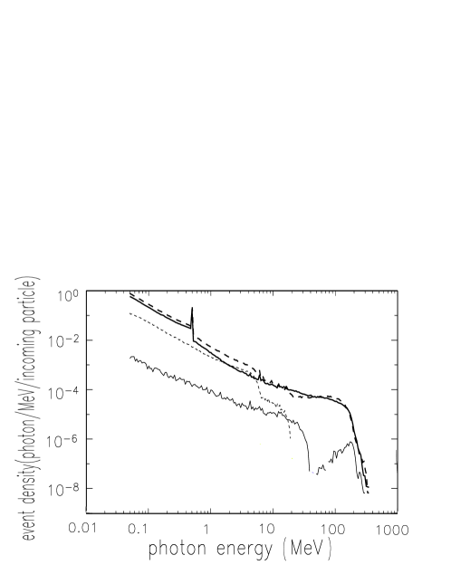
Figure 1.— A comparison between the nuclear de-excitation spectra generated with two different physics modules in GEANT4. The details of the simulation parameters are in the text. The thick and thin solid lines represent the total spectrum and the contribution of proton inelastic processes respectively, from the module HadronPhysicsQGSP_BERT_HP. The thick and thin dashed lines are from the module HadronPhysicsQGSP_BIC_HP.

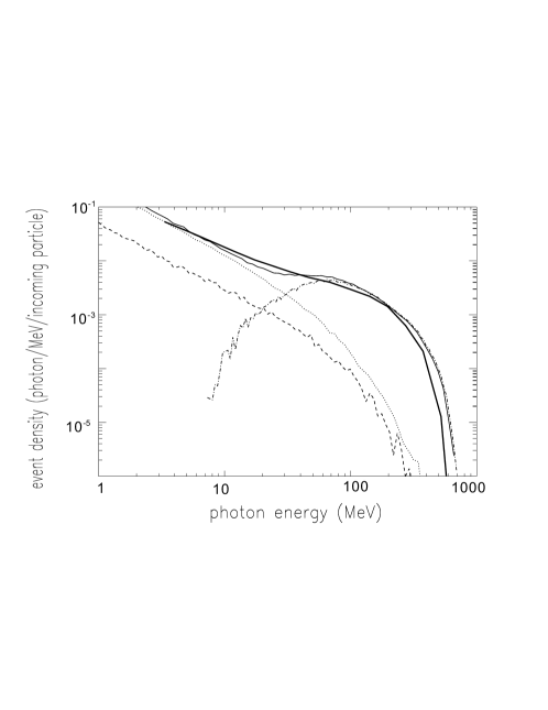
Figure 2.— A comparison between the pion-decay spectra generated with the HadronPhysicsQGSP_BERT_HP module of GEANT4 and the code developed at NRL by R. Murphy et al.; the HadronPhysicsQGSP_BIC_HP module gives similar results. Dash dot: $\pi^{0}$ decay. Dotted: bremsstrahlung of $e^{\pm}$ from the decay of $\pi^{\pm}$. Dashed: positron annihilation. Thin solid: the total spectrum from GEANT4. Thick solid: the total spectrum from the NRL code.

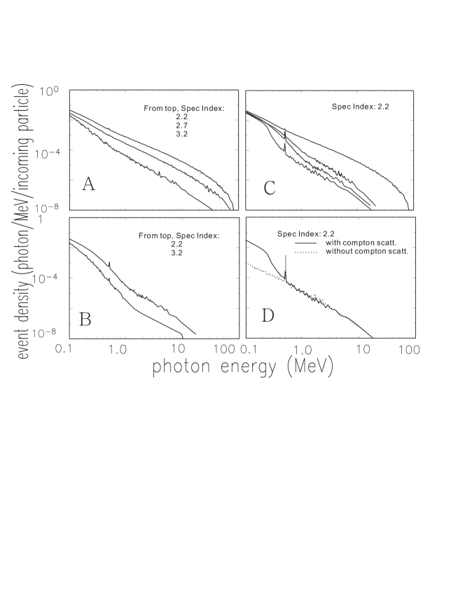
Figure 3.— The outgoing gamma-ray spectrum for different electron spectra and distributions. Panel A: Isotropic distribution. Panel B: Directly downward-beamed distribution. Panel C: the outgoing spectrum for different injected angular distributions with electron spectral index 2.2. From top down: (1) isotropic distribution; (2) pancake distribution uniform within angles $\theta$ such that $-0.3<\cos\theta<0.3$; (3) downward-isotropic distribution; and (4) downward-beamed distribution. Panel D: the gamma-ray spectrum from directly downward-beamed electrons with a spectral index 2.2, with the Compton scattering process turned on (solid) and off (dotted). All electron spectra are cut off at 0.1 MeV and 100 MeV and the outgoing spectra are collected at angles $\beta$ from the solar normal such that $\cos\beta>0.8$.

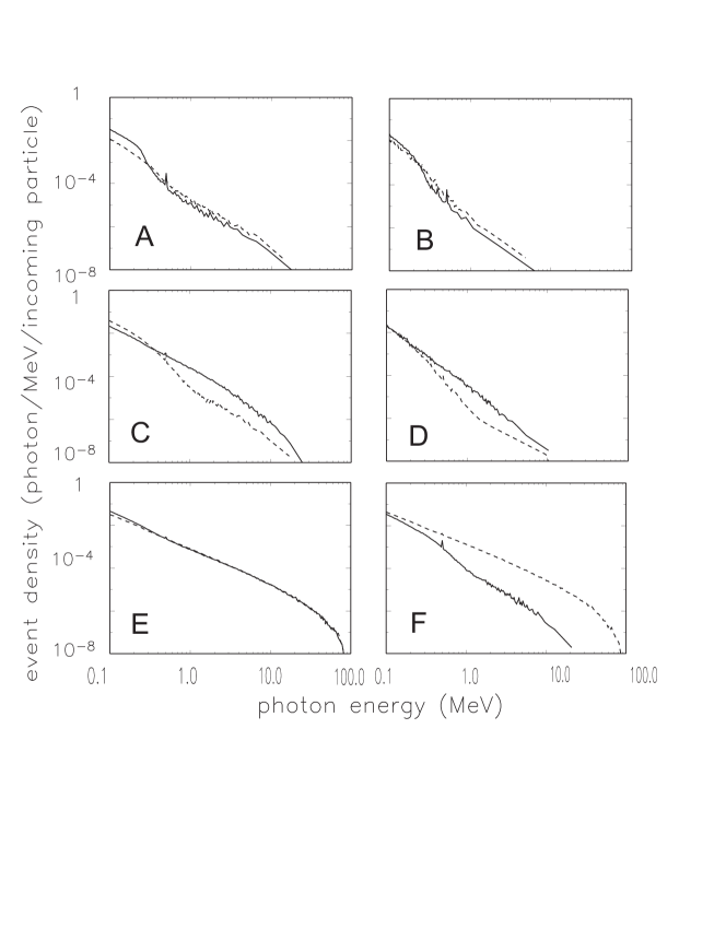
Figure 4.— The gamma-ray spectrum recorded at different outgoing angles $\beta$ from the solar normal. The solid line is $\cos\beta>0.8$ and the dashed line is $0.2<\cos\beta<0.4$. Panel A: downward-beamed distribution with spectral index 2.2. Panel B: downward-beamed distribution with spectral index 3.2. Panel C: downward-isotropic distribution with spectral index 2.2. Panel D: downward-isotropic distribution with spectral index 3.2. Panel E: isotropic distribution with spectral index 2.2. Panel F: pancake distribution with spectral index 2.2 (isotropic within angle $\theta$ of solar normal such that $-0.2<\cos\theta<0.2$).

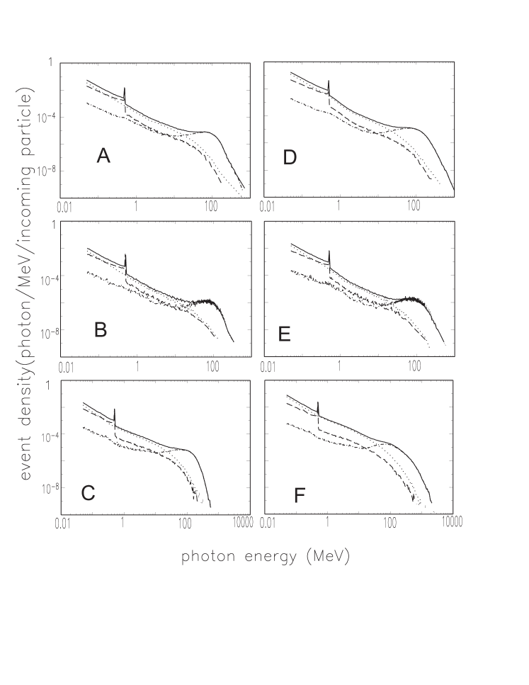
Figure 5.— The outgoing gamma-ray spectrum for different parameters of injected protons. Dash dot: $\pi^{0}$ decay. Dotted: bremsstrahlung of $e^{\pm}$ from the decay of $\pi^{\pm}$. Dashed: positron annihilation. Thin solid: the total spectrum. Panels A and B: downward-beamed distributions with spectral index 2.2 and 3.2, respectively. Panels D and E: downward-isotropic distributions with spectral indices 2.2 and 3.2, respectively. The above four panels are for $\cos\beta>0.8$. Panels C and F: downward-beamed and downward-isotropic distributions with spectral index 2.2, recorded at $0.2<\beta<0.4$. All proton spectra are cut off at 100 MeV and 10000 MeV.

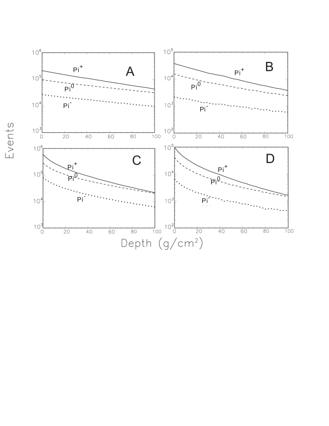
Figure 6.— The pion-producing depth distribution for different parameters of injected protons. Panels A and B: downward-beamed distributions with spectral indices 2.2 and 3.2, respectively. Panels C and D: downward-isotropic distributions with spectral indices 2.2 and 3.2, respectively. In each panel, solid: $\pi^{+}$; dashed: $\pi^{0}$; dotted: $\pi^{-}$.

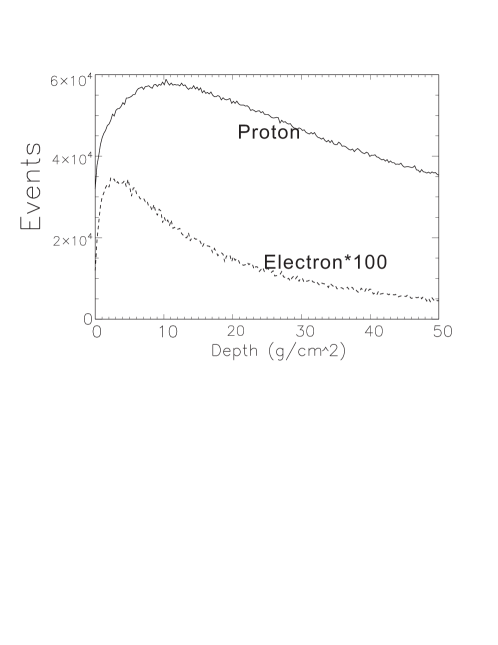
Figure 7.— The distribution of the depth where positron annihilation occurs. Solid line: positrons generated from injected protons. Dashed line: positrons generated from injected electrons. Both the electrons and protons follow a downward isotropic distribution with spectral index 2.2.

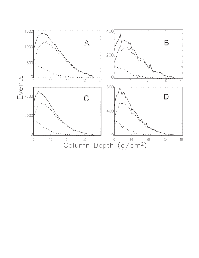
Figure 8.— The distribution of the depth where positron annihilation occurs, corresponding to photons collected at $\cos\beta>0.8$. Dashed line: photons that experience Compton scattering before being detected. Dotted line: photons that do not experience Compton scattering. Solid line: total. Panels A and B: downward beamed distributions with spectral indices 2.2 and 3.2, respectively. Panels C and D: downward isotropic distributions with spectral indices 2.2 and 3.2, respectively.

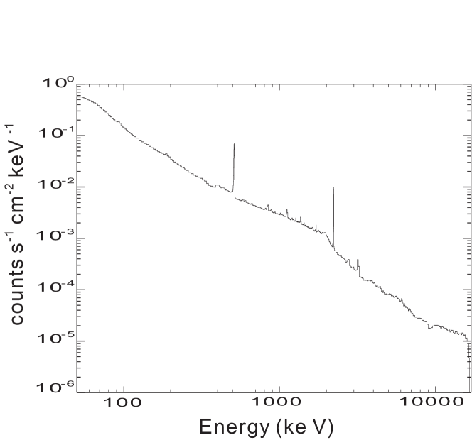
Figure 9.— The overall spectrum of the flare of 28 October 2003, from RHESSI (11:06 to 11:26 UT). A small discontinuity at 375 keV, a peak at 3 MeV, and a dip around 9 MeV are known instrumental artifacts that are accounted for when model spectra are fitted to these data. The effect of Compton scattering of solar photons in the instrument is most clearly seen at 2 MeV, where there is a shoulder due to Compton backscattering of 2.2 MeV neutron capture photons in RHESSI’s germanium detectors.

Figure 10.— The ratio between 511 keV line flux and the continua around 200 keV and 8–15 MeV, The meaning of different symbols are shown in the figure. From which, it is clear that if all the 511s are from proton and isotropically injected electrons, the 511/8–15 ratio would be well below observation and a combination of proton injection (plus symbol) and electron injection that is not complete isotropic (cross symbol) may produce the observation. See the text for more details.

References

- Agostinelli et al. (2003) Agostinelli, S., et al. 2003, NIMPA, 506, 250
- Arkhangelskaja et al. (2009) Arkhangelskaja, I. V., Kotov, Yu. D., Kalmykov, P. A., & Glyanenko, A. S., 2009, Advances in Space Research, 43, 589
- Aschwanden & Benz (1997) Aschwanden, M. J., & Benz, A. O., 1997, ApJ, 480, 825
- Bret (2009) Bret, A., 2009, ApJ, 699, 990
- Chin & Spyroui (2009) Chin, M. P. W., & Spyrou, N. M., 2009, Applied Radiation and Isotopes, 67, 406
- Dermer & Ramaty (1986) Dermer, C. D., & Ramaty, R., 1986, ApJ, 301, 962
- Forrest et al. (1980) Forrest, D. J., et al. 1980, Sol. Phys., 65, 15
- Gan (2004) Gan, W. Q., 2004, Sol. Phys., 219, 279
- Gingerich et al. (1971) Gingerich, O., Noyes, R. W., Kalkofen, W., & Cuny, Y., 1971, Sol. Phys., 18, 347
- Grevesse, Asplund & Sauval (2007) Grevesse, N., Asplund, M., & Sauval, A. J., 2007, Spaces. Sci. Rev., 130, 105
- Karlicky & Kasparova (2009) Karlicky, M., & Kasparova, J., A&A, 506, 1437
- Kontar & Brown (2006) Kontar, E. P., & Brown, J. C., ApJL, 653, L149
- Kontar et al. (2007) Kontar, E. P., Emslie, A. G., Massone, A. M., Piana, M., Brown, J. C., & Prato, M., 2007, ApJ, 670, 857
- Kotoku et al. (2007) Kotoku, J., Makishima, K., Matsumoto, Y., Kohama, M., Terada, Y., & Tamagawa, T., 2007, PASJ, 59, 1161
- Krucker et al. (2008) Krucker, S., Hurford, G. J., MacKinnon, A. L., Shih, A. Y., & Lin, R. P., 2008, ApJL, 687, L63
- Li et al. (1994) Li, P., Hurley, K., Barat, C., Niel, M., Talon, R., & Kurt, V., 1994, ApJ, 426, 758
- Li (1995) Li, P., 1995. ApJ, 443, 855
- Lin et al. (2002) Lin, R. P., et al. 2002, Sol. Phys., 210, 3
- Murphy & Ramaty (1984) Murphy, R. J., & Ramaty, R., 1984, Adv. Space. Res., 4, 127
- Murphy, Dermer & Ramaty (1987) Murphy, R. J., Dermer, C. D. & Ramaty, R., 1987, ApJS, 63, 721
- Murphy et al. (2005) Murphy, R. J., Share, G. H., Skibo, J. G., & Kozlovsky, B. 2005 ApJS, 161, 495
- Salvat, Fernandez-Varea & Sempau (2006) Salvat, F., Fernandez-Varea, J. M., & Sempau, J., PENELOPE-2006: A Code System for Monte Carlo Simulation of Electron and Photon Transport, Workshop Proceedings Barcelona, Spain, 4-7 July 2006
- Seltzer & Berger (1985) Seltzer, S. M. & Berger, M. J. 1985, Nuc. Inst. Meth. B., 12, 95
- Share & Murphy (1995) Share, G. H. & Murphy, R. J. 2005, ApJ, 452, 993
- Share et al. (2004) Share, G. H., Murphy, R. J., Smith, D. M., Schwartz, R. A., & Lin, R. P., 2004, ApJL, 615, L169
- Smith et al. (2002) Smith, D. M. et al. 2002, Solar Phys., 210, 33
- Smith et al. (2003) Smith, D. M., Share, G. H., Murphy, R. J., Schwartz, R. A., Shih, A. Y., & Lin, R. P., 2003, ApJL, 595, L81
- Vestrand et al. (1987) Vestrand, W. T., Forrest, D. J., Chupp, E. L., Rieger, E., & Share, G. H., 1987, ApJ, 322, 1010