E-loyalty networks in online auctions

Abstract

Creating a loyal customer base is one of the most important, and at the same time, most difficult tasks a company faces. Creating loyalty online (e-loyalty) is especially difficult since customers can “switch” to a competitor with the click of a mouse. In this paper we investigate e-loyalty in online auctions. Using a unique data set of over 30,000 auctions from one of the main consumer-to-consumer online auction houses, we propose a novel measure of e-loyalty via the associated network of transactions between bidders and sellers. Using a bipartite network of bidder and seller nodes, two nodes are linked when a bidder purchases from a seller and the number of repeat-purchases determines the strength of that link. We employ ideas from functional principal component analysis to derive, from this network, the loyalty distribution which measures the perceived loyalty of every individual seller, and associated loyalty scores which summarize this distribution in a parsimonious way. We then investigate the effect of loyalty on the outcome of an auction. In doing so, we are confronted with several statistical challenges in that standard statistical models lead to a misrepresentation of the data and a violation of the model assumptions. The reason is that loyalty networks result in an extreme clustering of the data, with few high-volume sellers accounting for most of the individual transactions. We investigate several remedies to the clustering problem and conclude that loyalty networks consist of very distinct segments that can best be understood individually.

and

1 Introduction

Online auctions are becoming an increasingly important component of consumers’ shopping experience. On eBay, for instance, several million items are offered for sale every day. What makes online auctions popular forms of commerce is their availability of almost any kind of item, whether it be new or used, and their constant accessibility at any time of the day, from any geographical region in the world. Moreover, the auction mechanism often engages participants in a competitive environment and can result in advantages for both the buyers and the sellers [Bajari and Hortacsu (2004)].

In this paper we study online auctions from the point of view of the bidder–seller network that they induce. Every time a bidder purchases from a seller, both bidder and seller are linked. Buying from a seller indicates that the bidder likes the product and trusts the seller—thus, it establishes a relationship between bidder and seller. Many sellers list more than one auction (i.e., they sell multiple items across different auctions), so repeat transactions by the same bidder across different auctions of the same seller measure the strength of this relationship, that is, it measures the strength of a bidder’s loyalty to a particular seller.

Studying loyalty in auction networks is new. Much of the existing auction literature focuses on only the seller and the level of trust she signals to the bidders [e.g., Brown and Morgan (2006)]. To that end, a seller’s feedback score (i.e., the number of positive ratings minus the number of negative ratings) is often scrutinized [e.g., Lingfang (2006)] and it has been shown that higher feedback scores can lead to price-premiums for the seller [see Lucking-Reiley et al. (2007); Livingston (2005)]. In this paper we study a complementary determinant of a bidder’s decision process: loyalty. Loyalty is different from trust. Trust is often associated with reliability or honesty; and trust may be a necessary (but not sufficient) prerequisite for loyalty. Loyalty, however, is a stronger determinant of a bidder’s decision process than trust. Loyalty refers to a state of being faithful or committed. Loyalty incorporates not only the level of confidence in the outcome of the transaction, but also satisfaction with the product, the price, and also with previous transactions by the same seller. Moreover, loyal bidders are often willing to make an emotional investment or even a small sacrifice to strengthen a relationship. This paper makes two contributions to the literature on online auctions: First, we propose a novel way to measure e-loyalty from the bipartite network of bidders and sellers; then, we investigate the effect of e-loyalty on the outcome of an auction and the statistical challenges associated with it.

More specifically, our goal is to understand and learn from loyalty networks. To that end, we first measure a seller’s perceived loyalty by its induced bidder loyalty distribution. Then, borrowing ideas from functional data analysis, we capture key elements of that distribution using functional principal component analysis. The resulting principal component scores capture different aspects of loyalty-strength, -skew and -variability. We then investigate the impact of these loyalty scores on the outcome of an auction such as its final price.

We would like to point out that the goal of this paper is not to develop new auction theory (i.e., it is not our goal to develop a game-theoretic model under market equilibrium considerations). Rather, our goal is to mine a rich set of auction data for new patterns and knowledge. In that sense, our work is exploratory rather than confirmatory. However, as it is often the case with exploratory work, we hope that our work will also inspire the development of new theory. In particular, we hope that our work will bring the attention to the many statistical challenges associated with the study of online markets.

Studying e-loyalty networks is challenging from a statistical point of view because of the asymmetric nature of the network. Just as in many offline markets, online auctions are dominated by few very large sellers (“Megasellers”). Megasellers have a large supply of products and thus account for a large number of all the transactions. Statistically, this dominance results in a clustering of the data and, as a result, a violation of standard OLS model assumptions. In this paper we investigate several remedies to this clustering effect via random effects models and weighted least squares. However, our investigation shows that neither approach fully eases all problems. We thus conclude that the data is too segmented to be captured by a single model and compare our analyses with the results of a data-clustering approach.

This paper has implications for future research in online markets. Many online markets are characterized by a few large “players” that dominate most of the interactions and many, many small players with occasional interactions. This is often referred to as the “long tail effect” in online markets [see, e.g., Bailey et al. (2008)]. For instance, on eBay, Megasellers dominate the marketplace. The statistical implication is that repeat interactions by these Megasellers are no longer independent and, hence, the assumptions of OLS break down. While this may not always create a problem, this research shows that, first, the conclusions from an OLS regression are significantly different from models that account for the clustering induced by Megasellers, and, second, that it is not at all obvious how to best account for this clustering. In particular, this research puts the spotlight on the findings from previous researchers [e.g., Lucking-Reiley et al. (2007); Ba and Pavlou (2002); Bapna, Jank and Shmueli (2008)] who, despite similar data-scenarios, rely their conclusions on the OLS modeling assumptions. [See also Bajari and Hortacsu (2004) who, in the context of trust and online auctions alone, count over 6 papers relying on OLS modeling techniques.]

This paper is organized as follows. In Section 2 we introduce our data and we motivate the existence of auction networks. In Section 3 we use seller–bidder networks to derive several key measures of e-loyalty. We investigate the effect of e-loyalty on the outcome of an auction in Section 4 and explore different modeling alternatives. The paper concludes with final remarks in Section 5.

2 Auction networks

In this section we describe the data for our study. We start by describing the online auction mechanism in general and our data in particular. Then, we motivate the network structure induced by the auction mechanism and show several snapshots of our network data.

2.1 Online auction data

In online auctions participants bid for products or services over the Internet. While there are different types of auction mechanisms, one of the most popular types (a variant of which can also be found on eBay.com) is the Vickrey auction, in which the initial price starts low and is bid up successively. Online auctions have experienced a tremendous popularity recently, which can be attributed to several features: Since the auction happens online, it is not bound by any temporal or geographical constraints, in stark contrast to its brick-and-mortar counterpart (e.g., at Sotheby’s). It also fosters social interactions since it engages participants in a competition. As a result, it attracts a large number of buyers and sellers which offers advantages for both sides: sellers find a large number of potential customers which often results in higher prices and lower costs. On the other hand, buyers find a large variety of products which enables them to locate rare products and to choose between products with the lowest price. One of the most well-known online auctions is eBay, but there are many more (e.g., uBid, Prosper, Swoopo or Overstock), each of which offers a variety of different products and services. The data for this research originates from eBay online auctions and we describe details of the data next.

Table 1: Auctions and products

Attribute	Mean	Median	St. dev
Auction duration (Days)	$3.50$	$3.00$	$4.43$
Starting price (USD)	$3.77$	$3.33$	$5.64$
Closing price (USD)	$6.61$	$4.25$	$9.15$
Item quantity	$5.42$	$1.00$	$129.47$
Bid count	$3.16$	$1.00$	$4.26$
Size (bead diameter)	$6.41$	$6.00$	$3.35$
Pieces (# of beads per item)	$124.30$	$48.00$	$343.79$

Table 2: Sellers

Attribute	Mean	Median	St. dev
Volume	$163.90$	$6.00$	$999.00$
Conversion rate	$0.67$	$0.67$	$0.33$
Seller feedback	$2054.00$	$264.00$	$12\mbox{,}400.00$

We study the complete bidding records of Swarovski fine beads for every single auction that was listed on eBay between April, 2007, and January, 2008. (Note that the data were obtained directly from eBay so we have a complete set of bidding records for that time frame.) Our data contains a total of 36,728 auctions out of which 25,314 transacted. There are 365 unique sellers and 40,084 bidders out of which 19,462 made more than a single purchase. Each bidding record contains information on the auction format, the seller, the bidder, as well as on product details. Tables 1–3 summarize this information.

Table 1 shows information about the auctions and the product sold in each auction. We can see that the typical auction-length is 3 days. The product sold in each auction (packages of beads for crafts and artisanship) is of relatively small value and, thus, both the average starting and closing prices are low. While many eBay auctions sell only one item at a time (e.g., laptop or automobile auctions), auctions in the crafts category often feature multi-unit auctions, that is, the seller offers multiple counts of the same item and bidders can decide how many of these items they wish to purchase. In our data the average item-quantity per auction is 5.42. Auctions thrive under competition among bidders and while the average number of bids is slightly larger than 3, the median is only 1. As pointed out above, the items sold in these auctions are packages of Swarovski beads. The value of a bead is, in part, defined by its size, and the average diameter of our beads equals 6.41 millimeters. Another measure for the value of an item is the number of pieces per package; we can see that there are on average over 124 beads in each package, but this number varies significantly from auction to auction.

Table 3: Buyers

Attribute	Mean	Median	St. dev
Volume	$3.62$	$1.00$	$14.29$
Item quantity	$5.05$	$2.00$	$29.25$
Bidder feedback	$228.10$	$70.00$	$559.53$

We are primarily interested in the bipartite network between bidders and sellers. One main factor influencing this network is the size of the seller. We can see (Table 2) that the average seller-volume (i.e., number of auctions per seller) is over 163. A seller’s auction will only transact if (at least one) bidder places a bid. While low transaction rates (or “conversion rates”) are a problem for many eBay categories (e.g., automobiles), in our data the average conversion rate is 67% per seller, which is considerably high. One factor driving conversion rates is a seller’s perceived level of trust. Trust is often measured using a seller’s feedback rating computed as the sum of positive (“$+$”) and negative (“$-$”) ratings. Trust averages over 2000 in our data.

Table 3 shows the corresponding attributes of the bidders. Bidders win on average almost 4 auctions (“volume”) and, in every auction, they purchase on average over 5 items. (Recall the multi-unit auctions with several items per listing.) The bidder feedback [computed as the sum of positive (“$+$”) and negative (“$-$”) feedback] captures a bidder’s experience with the auction-process and its average is over 220 in our data, signaling highly experienced bidders.

2.2 Bidder–seller networks

Interactions in an online auction result in a network linking its participants. Bidders bidding on one auction are linked to other bidders who bid on the same auction. Sellers selling a certain product are linked to other sellers selling the same product. In this study we focus on the network between buyers and sellers. Each time a bidder transacts with a particular seller, both are linked. A seller can set up more than one auction, thus, repeat transactions (i.e., purchases) measure the strength of this link. For instance, a bidder transacting 10 times with the same seller has a stronger link compared to a bidder who transacts only twice. In our analyses, we only consider edges with link-strength of at least 4. That is, we disregard all bidder–seller transactions with frequency less than 4. While there exists no recommended or ideal cut-off, our investigations suggest that results vary for smaller values but stabilize for link-strengths of 4 and higher. In that sense, the network strength measures an important aspect about the relationship between buyers and sellers: customer loyalty.

We would like to emphasize that one can measure loyalty in different ways. While one could count all the repeat bids a bidder places on auctions hosted by the same seller, we only count the number of winning bids (i.e., the number of transactions). While both bids and winning bids indicate a relationship between buyers and sellers, a winning bid signals a much stronger commitment and is thus much more indicative of a buyer’s loyalty.

In this paper we investigate loyalty relationships across auctions. Studying cross-auction relationships is rather rare in the literature on online auctions, and it has gained momentum only recently [Haruvy et al. (2008); Reddy and Dass (2006); Jank and Shmueli (2007); Jank and Zhang (2008)]. In this work we consider network effects between auction participants and their impact on the outcome of an auction.

Consider Figure 1 which shows the top 10% of high volume sellers. Sellers are marked by white triangles, bidders are marked by red squares. A (black) line between a seller and bidder denotes a transaction. The width of the line is proportional to the number of transactions and hence measures the strength of a link. We can see that some sellers interact with several hundred different bidders (with 895, on average); we can also see that some sellers are “exclusive” in the sense that they are the only ones that transact with a set of bidders (see, e.g., at the margins of the network), while other sellers “share” are a common set of bidders. Serving bidders exclusively vs. sharing them with other sellers has huge implications on the outcome of the auction.

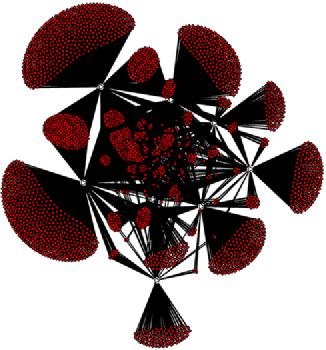
Figure 1: Network of the top 10th percentile of sellers: the top 10% of sellers hosting the most auctions.

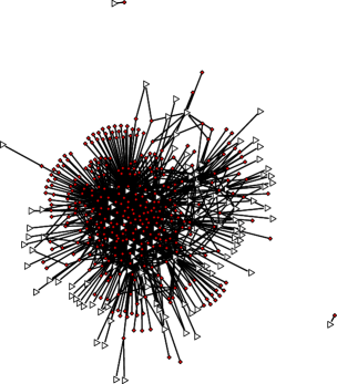
Figure 2: Network of the top 10th percentile of bidders: the top 10% of bidders bidding on most auctions.

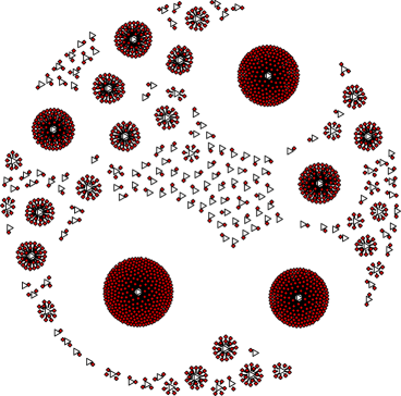
Figure 3: Network of new bidders: Bidders who bid for the very first time.

Figure 2 shows another subset of the data. In this figure we display only the top 10% of all bidders with the highest number of transactions. We can see that many of these high-volume bidders transact with only one seller (note the many the red triangles which are connected with only a single arc to the network) and are hence very loyal to the same person. Figure 3 shows only new buyers (i.e., bidders who won an auction for the first time). This network exemplifies the market share of a seller with the effect of repeat buyers removed. We can see that the market is dominated by few mega sellers, yet smaller sellers still attract some of the buyers. We can identify 5 mega-sellers, 3 high-volume sellers, and many medium- and low-volume sellers. Since these are only first-time buyers, loyalty does not yet play a role in bidders’ decisions. However, the fact that most first-time bidders “converge” to only a few mega-sellers suggests that this is a very difficult market for low-volume sellers to enter.

As pointed out above, bidder–seller networks capture loyalty of participants. While most sellers and bidders are linked to one another, here we only focus on the sub-graphs created by each bidder–seller pair. Next, we describe an innovative way to extract loyalty measures from these graphs.

3 Extracting loyalty from network information

Our loyalty measures map the entire network of bidders and sellers into a few seller-specific numbers. For each seller, these numbers capture both the proportion of bidders loyal to that seller, as well as the degree of loyalty of each bidder. We derive the measure in two steps. First, we derive, for each seller, the loyalty distribution; then, we summarize that distribution in a few numbers using functional principal component analysis. We describe each step in detail below.

Note that there exists more than one way for extracting loyalty information from network data. We chose the route of loyalty distributions since they capture the two most important elements of loyalty: the proportion of customers loyal to one’s business, and the degree of their loyalty. Notice, in particular, that we do not try to dichotomize loyalty (i.e., categorize it into loyal vs. disloyal buyers): Since we do not believe that loyalty can be turned on or off arbitrarily, we allow it to range on a continuous scale between 0 and 1. This will allow us to quantify the impact of the shape of a seller’s loyalty distribution on his or her bottom line. For instance, it will allow us to answer whether sellers with pure loyalty (i.e., all buyers 100% loyal) are better off compared to sellers with more variation among their customer base.

We would also like to caution that the resulting analysis is complex since we first have to characterize the infinite-dimensional loyalty distributions in a finite way, and subsequently interpret the resulting characterizations. The resulting interpretations are more complex than, say, employing user-defined measures of loyalty (e.g., summary statistics such as the number of loyal buyers or the proportion of at least 70% loyal buyers). While such user-defined measures are easy to interpret, there is no guarantee that they capture all of the relevant information. (For instance, measuring the “number of loyal bidders” would first require us to define a cutoff at which we consider one buyer to be loyal and another one to be disloyal—any such cutoff is necessarily arbitrary and would lead to a dichotomization which we are trying to avoid.) Rather than employing arbitrary, user-defined measures, we set out to let the data speak freely and first look for ways to summarize the information captured in the loyalty distributions in the most exhaustive way. This will lead us to the notion of principal component loyalty scores and their interpretations. We will elaborate on both aspects below.

3.1 From loyalty networks to loyalty distributions

Consider the hypothetical seller–bidder network in Figure 4. In that network, we have 4 sellers (labeled “A,” “B,” “C” and “D”) and 10 bidders (labeled 1–10). An arc between a seller–bidder pair denotes an interaction, and the width of the arc is proportional to the number of repeat-interactions between the pair. Consider bidder 1 who has a total of 10 interactions, all of which are with seller A; we can say that bidder 1 is 100% loyal to seller A. This is similar for bidders 2 and 3, who have a total of 8 and 6 interactions, respectively, all of which are, again, with seller A. In contrast, bidders 4 and 5 are only 80% and 70% loyal to seller A since, out of their total number of interactions (both 10), they share 2 with seller B and 3 with seller C, respectively. All-in-all, seller A attracts mostly highly loyal bidders. This is different for seller D who attracts mostly little loyal bidders, as he shares all of his bidders with either seller B or C.

(a)

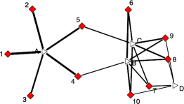
(b)

Figure 4: (a) Shows a hypothetical network between 4 sellers (A–D, white triangles) and 10 bidders (1–10, red squares). The size of the arc between a seller and a bidder corresponds to the number of interactions between the two. (b) Shows the resulting loyalty distributions for each seller (i.e., it shows the relative frequencies).

For each seller, we can summarize the proportion of loyal bidders and the degree of their loyalty in the associated loyalty distribution. The loyalty distributions for sellers A–D are displayed in the right panel of Figure 4. The $x$-axis denotes the degree of loyalty (e.g., 100% or 80% loyal), and the $y$-axis denotes the corresponding density. We can see that the shape of all four distributions is very different; while seller A’s distribution is very left-skewed (mostly high-loyal bidders), seller D’s distribution is very right-skewed (mostly little-loyal bidders). The distributions of sellers B and C fall somewhat in between, yet they are still very distinct from one another.

Note that our definition of loyalty is similar to the concept of in- and out-degree analysis. More precisely, we first measure the proportion of interactions for each buyer (i.e., the normalized distribution of out-degree). Then, we measure the perceived loyalty of each seller, which can be viewed as the distribution of the weighted in-degree. This definition of loyalty is very similar to the concept of brand-switching in marketing. In essence, if we have a fixed number of brands (sellers in our case) and a pool of buyers (i.e., bidders), then we measure the switching-behavior from one brand to another.

While the loyalty distributions in Figure 4 capture all of the relevant information, we cannot use them for further analysis (especially modeling). Thus, our next step is to characterize each loyalty distribution by only a few numbers. To that end, we employ a very flexible dimension reduction approach via functional data analysis.

3.2 From loyalty distributions to loyalty measures

In order to investigate the effect of loyalty on the outcome of an auction, we first need to characterize a seller’s loyalty distribution. While one could characterize the distributions via summary statistics (e.g., mean, median or mode), Figure 4 suggests that loyalty is too heterogeneous and too dispersed. Therefore, we resort to a very flexible alternative via functional data analysis [Ramsay and Silverman (2005)].

By functional data we mean a collection of continuous functional objects such as curves, shapes or images. Examples include measurements of individuals’ behavior over time, digitized 2- or 3-dimensional images of the brain, or recordings of 3- or even 4-dimensional movements of objects traveling through space and time. In our application, we regard each seller’s loyalty distribution as a functional observation. We capture similarities (and differences) across distributions via functional principal component analysis (fPCA), a functional version of principal component analysis [see Kneip and Utikal (2001)]. In fact, while Kneip and Utikal (2001) operate on the true probability distributions, these are not known in our case; hence, we apply fPCA to the observed (empirical) distribution function, which may introduce an extra level of estimation error.

Functional principal component analysis is similar in nature to ordinary PCA; however, rather than operating on data-vectors, it operates on functional objects. In our context, we take the observed loyalty distributions [i.e., the histograms Figure 4(b)] as input. While one could also first smooth the observed histograms, we decided against it since the results were not substantially different.

Ordinary PCA operates on a set of data-vectors, say, ${\mathbf{x}}_{1},\dots,{\mathbf{x}}_{n}$, where each observation is a $p$-dimensional data-vector ${\mathbf{x}}_{i}=(x_{i1},\dots,x_{ip})^{\mathrm{T}}$. The goal of ordinary PCA is to find a projection of ${\mathbf{x}}_{1},\dots,{\mathbf{x}}_{n}$ into a new space which maximizes the variance along each component of the new space and at the same time renders the individual components of the new space orthogonal to one another. In other words, the goal of ordinary PCA is to find a PC vector ${\mathbf{e}}_{1}=(e_{11},\dots,e_{1p})^{\mathrm{T}}$ for which the principal component scores (PCS)

$$S_{i1}=\sum_{j}e_{1j}x_{ij}={\mathbf{e}}_{1}^{\mathrm{T}}{\mathbf{x}}_{i}$$ (1)

maximize $\sum_{i}S_{i1}^{2}$ subject to

$$\sum_{j}e_{1j}^{2}=\|{\mathbf{e}}_{1}\|^{2}=1.$$ (2)

This yields the first PC, ${\mathbf{e}}_{1}$. In the next step we compute the second PC, ${\mathbf{e}}_{2}=(e_{21},\dots,e_{2p})^{\mathrm{T}}$, for which, similarly to above, the principal component scores $S_{i2}={\mathbf{e}}_{2}^{\mathrm{T}}{\mathbf{x}}_{i}$ maximize $\sum_{i}S_{i2}^{2}$ subject to $\|{\mathbf{e}}_{2}\|^{2}=1$ and the additional constraint

$$\sum_{j}e_{2j}e_{1j}={\mathbf{e}}_{2}^{\mathrm{T}}{\mathbf{e}}_{1}=0.$$ (3)

This second constraint ensures that the resulting principal components are orthogonal. This process is repeated for the remaining PC, ${\mathbf{e}}_{3},\dots,{\mathbf{e}}_{p}$.

The functional version of PCA is similar in nature, except that we now operate on a set of continuous curves rather than discrete vectors. As a consequence, summation is replaced by integration. More specifically, assume that we have a set of curves ${\mathbf{x}}_{1}(s),\dots,{\mathbf{x}}_{n}(s)$, each measured on a continuous scale indexed by $s$. The goal is now to find a corresponding set of PC curves, ${\mathbf{e}}_{i}(s)$, that, as previously, maximize the variance along each component and are orthogonal to one another. In other words, we first find the PC function, ${\mathbf{e}}_{1}(s)$, whose PCS

$$S_{i1}=\int e_{1}(s)x_{i}(s)\,ds$$ (4)

maximize $\sum_{i}S_{i1}^{2}$ subject to

$$\int e_{1}^{2}\,ds=\|{\mathbf{e}}_{1}\|^{2}=1.$$ (5)

Similarly to the discrete case, the next step involves finding ${\mathbf{e}}_{2}$ for which the PCS $S_{i2}=\int e_{2}(s)x_{i}(s)\,ds$ maximize $\sum_{i}S_{i2}^{2}$ subject to $\|{\mathbf{e}}_{2}\|^{2}=1$ and the additional constraint

$$\int e_{2}(s)e_{1}(s)\,ds=0.$$ (6)

In practice, the integrals in (4)–(6) are approximated either by sampling the predictors, ${\mathbf{x}}_{i}(s)$, on a fine grid or, alternatively, by finding a lower-dimensional expression for the PC functions ${\mathbf{e}}_{i}(s)$ with the help of a basis expansion. For instance, let ${\bolds{\phi}}(s)=(\phi_{1}(s),\dots,\phi_{K}(s))$ be a suitable basis expansion [Ramsay and Silverman (2005)], then we can write

$${\mathbf{e}}_{i}(s)=\sum_{k=1}^{K}b_{ik}\phi_{k}(s)={\bolds{\phi}}(s)^{\mathrm{T}}{\mathbf{b}}_{i}$$ (7)

for a set of basis coefficients ${\mathbf{b}}=(b_{i1},\dots,b_{iK})$. In that fashion, the integral in, for example, (6) becomes

$$\int e_{2}(s)e_{1}(s)\,ds={\mathbf{b}}_{1}^{\mathrm{T}}{\mathbf{W}}{\mathbf{b}}_{2},$$ (8)

where ${\mathbf{W}}=\int{\bolds{\phi}}(s){\bolds{\phi}}(s)^{\mathrm{T}}\,ds$. For more details, see Ramsay and Silverman (2005). In this work we use the grid-approach.

Figure 5: First two principal component curves. The dashed line indicates the $x$-origin.

Common practice is to choose only those eigenvectors that correspond to the largest eigenvalues, that is, those that explain most of the variation in ${\mathbf{x}}_{1}(s),\dots,{\mathbf{x}}_{n}(s)$. By discarding those eigenvectors that explain no or only a very small proportion of the variation, we capture the most important characteristics of the observed data patterns without much loss of information. In our context, the first 2 eigenvectors capture over 82% of the variation in loyalty distributions.

3.3 Interpreting the loyalty measures

Since our loyalty measures are based on their principal component representations, interpretation has to be done with care. Figure 5 shows the first 2 principal components (PCs). The first PC (top panel) shows a growing trend and, in particular, it puts large negative weight on the lowest loyalty scores (between 0 and 0.2) while putting positive weight on medium to high loyalty scores (0.4 and higher). Thus, we can say that the first PC contrasts the extremely disloyal distributions from the rest. Table 4 (first row) confirms this notion: Notice the large negative correlation with the minimum; also, the large correlation with the skewness indicates that PC1 truly captures extremes in the loyalty distributions’ scores and shape. We can conclude that PC1 distinguishes distributions of “pure disloyalty” from the rest.

The second PC has a different shape. The second PC puts most (positive) weight on the highest loyalty scores (between 0.8 and 1); it puts negative weight on scores at the medium and low scores (between 0.4 and 0.6) and thus contrasts average loyalty from extremely high loyalty. Indeed, Table 4 (second row) shows that PC2 has a high positive correlation with the maximum and a high negative correlation with the median. In that sense, it distinguishes the mediocre loyalty from the stars.

While the above interpretations help our understanding of the loyalty components, their overall impact is still hard to grasp, especially because every individual loyalty distribution will—by nature of the principal component decomposition—comprise of a different mix between PC1 and PC2. Moreover, as we apply fPCA to observed densities (i.e., histograms), individual values of each density function must be heavily correlated. This adds additional constraints on the PCs and their interpretations. Hence, in the following, we discuss five theoretical loyalty distributions and their corresponding representation via PC1 and PC2.

=210pt Median SDev Max Min Skew PC1 $0.55$ $-0.2$ 0.52 $-0.99$ 0.77 PC2 $-0.78$ $-0.05$ 0.81 $-0.02$ 0.63

Table 4: Correlation between the first two PC scores and summary statistics of sellers’ loyalty distributions

Figure 6: Five theoretic loyalty distributions.

Take a look at Figure 6. It shows five plausible loyalty distributions as they may develop out of a bidder–seller network. We refer to these distributions as “theoretic loyalty distributions” and we can characterize them by their specific shapes. For instance, the first distribution is comprised of 100% loyal buyers and we hence refer to it as “pure loyalty;” in contrast, the last distribution is comprised of 100% disloyal buyers and we hence name this distribution “pure disloyalty;” the distribution in the center (“somewhat loyal”) is interesting since it is comprised mostly of buyers that exhibit some loyalty but do not purchase exclusively from only one seller.

Table 5 shows the corresponding PC scores. We can see that the theoretical distribution corresponding to pure loyalty scores very high on PC1 since it is very right-skewed and does not have any values lower than 0.9; in contrast, notice the PC1 scores for pure disloyalty: while it is the mirror image of pure loyalty, it scores (in absolute terms) higher than the former because it is not only very (left-) skewed, but its extremely small values weigh heavily (and negatively) with the first part of the PC1-shape, which is in contrast to the positive values of pure loyalty which do not receive as much weight. As for PC2, Table 5 shows that pure loyalty scores even higher on that component as its values are extremely large, much larger than the typical (median) loyalty values. In contrast, pure disloyalty has very small PC2 values, as low scores are given very little weight by PC2.

Table 5: PC1 and PC2 scores for the theoretical loyalty distributions from Figure 6

	Pure lyty	Strong lyty	Somewhat loyal	Two extremes	Pure dislyty
PC1	0.56	0.47	$0.32$	$-0.04$	$-0.64$
PC2	0.72	0.51	$-0.08$	$0.35$	$-0.01$

We can make similar observations for the remaining theoretical loyalty distributions. For instance, the distribution of somewhat loyal scores high on PC1 since it does not have many low values; but it also only receives an average score on PC2 since it does not have many high values either. In the following, we will use these theoretical loyalty distributions to shed more light on the relationship between loyalty and the outcome of an auction.

4 Modeling e-loyalty

Our goal is to investigate the effect of loyalty on the outcome of an auction. For instance, we would like to see whether sellers who attract exclusively high-loyal bidders elicit price-premiums, or whether more variability in buyers’ loyalty leads to a higher price. To that end, we start out, in similar fashion to many previous studies on online auctions [e.g., Lucking-Reiley et al. (2007)], with an ordinary least squares (OLS) modeling framework. That is, we investigate a model of the form

$${\mathbf{y}}={\mathbf{X}}{\bolds\beta}+{\bolds\varepsilon},$$ (9)

where ${\mathbf{X}}$ is a matrix of covariates and ${\bolds\varepsilon}$ follows the standard linear model assumptions. For the choice of the covariates, we are primarily interested in the effect of loyalty on the price of an auction (i.e., the first 2 PC scores from the previous section are our main interest). However, we also want to control for factors other than loyalty which are also known to have an impact on price; these factors include auction characteristics (auction duration), item characteristics (item quantity, size and pieces), seller characteristics (seller feedback, i.e., reputation and seller volume) and auction competition (number of bids, i.e., bid-count).

We first investigate a standard OLS model that relates these covariates to price. However, we will show that an OLS approach leads to violations of the model assumptions. The reason lies in the asymmetry of the bidder–seller network: the presence of high-volume sellers (i.e., seller nodes with extremely high degree) biases the analysis and leads to wrong conclusions. In particular, high-volume sellers have many repeat interactions which result in a strong clustering of the data and thus violate the i.i.d. assumption of OLS. We investigate several remedies to this problem. First, we investigate two “standard” remedies via random effect (RE) models and weighted least squares (WLS). Our results show that although both remedies ease the problem, none removes it completely. We thus argue that the data is too heterogeneous to be modeled within a single model and compare our results with that of a data-segmentation strategy.

4.1 An initial model: OLS

Many studies employ an OLS modeling framework to investigate phenomena in online auctions such as the effect of the auction format, the impact of a seller’s reputation, or the amount of competition [e.g., Lucking-Reiley et al. (2007); Ba and Pavlou (2002); Bapna, Jank and Shmueli (2008)]. However, one problem with an OLS model approach is the presence of repeat observations on the same item. For instance, if we want to study the effect of a seller’s reputation (measured by her feedback score), then repeat auctions by the same seller will severely overweight the effect of high-volume sellers in the OLS model. This problem is typically not addressed in the online auction literature. We face a very similar problem when modeling the effect of e-loyalty.

Table 6: Regression models on the entire (unsegmented) data set. The top panel shows the results of OLS regression; the middle panel shows the random effects model, and the bottom panel shows the weighted least squares model. The response is always log-price

Coefficient	Estimate	Std. error	$\bolds p$-value
(Intercept)	$-1.64$	0.06	0.00
Auction duration	$0.02$	0.00	0.00
log(item quantity $+$ 1)	$-0.04$	0.04	0.30
Bid count	$0.06$	0.00	0.00
log(Pieces)	$0.42$	0.00	0.00
Size	$0.07$	0.00	0.00
log(seller feedback $+$ 1)	$-0.00$	0.01	0.52
Loyalty-PC1	$-0.17$	0.05	0.00
Loyalty-PC2	$-1.00$	0.07	0.00
log(Volume)	$0.16$	0.01	0.00
AIC	15,148
$R$-squared	$0.77$
(Intercept)	$-0.58$	0.22	0.00
Auction duration	$0.01$	0.00	0.00
log(item quantity $+$ 1)	$-0.21$	0.07	0.00
Bid count	$0.05$	0.00	0.00
log(Pieces)	$0.27$	0.00	0.00
Size	$0.03$	0.00	0.00
log(seller feedback $+$ 1)	$0.07$	0.04	0.11
Loyalty-PC1	$-0.40$	0.22	0.07
Loyalty-PC2	$-0.15$	0.22	0.51
log(Volume)	$0.05$	0.04	0.20
AIC	8546
$R$-squared	N/A
(Intercept)	$-1.59$	0.12	0.00
Auction duration	$0.01$	0.00	0.01
log(item quantity $+$ 1)	$0.30$	0.10	0.00
Bid count	$0.08$	0.00	0.00
log(Pieces)	$0.26$	0.01	0.00
Size	$0.00$	0.00	0.61
log(seller feedback $+$ 1)	$-0.01$	0.01	0.59
Loyalty-PC1	$-1.00$	0.08	0.00
Loyalty-PC2	$1.33$	0.11	0.00
log(Volume)	$0.24$	0.01	0.00
AIC	55,073
$R$-squared	$0.43$

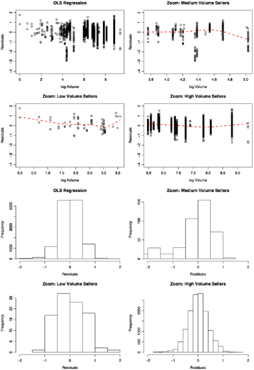
Figure 7: Residuals of the OLS model.

For illustration, take the OLS regression model in the top panel of Table 6. In this model we estimate the dependency of (log-)price on loyalty (measured by PC1 and PC2), controlling for all other factors described above. Note that this model appears to fit the data very well ($R$-squared $=$ 77%). However, it is curious to see that seller feedback has a negative sign and is statistically insignificant. This contradicts previous findings which found that an increased level of trust leads to price premiums [Bajari and Hortacsu (2004); Ba and Pavlou (2002); Lucking-Reiley et al. (2007)].

Figure 7 shows the residuals corresponding to the above model. The top half shows the residuals plotted against seller-volume; the bottom half shows the residual distribution. For each type of graph we present 4 different views: one graph (left graphs in first and third panel) gives an overview; the other graphs zoom in by seller volume (low, medium and high volume, respectively). Notice that the residuals are rather skewed: a large proportion of residuals are negative (see, e.g., top left graph), implying that our model over-estimates price effects of loyalty. Moreover, we can also see that the residual-variation increases for larger seller volumes. If we zoom in on both the low-volume and medium-volume sellers, we can see that the true effect of model misspecification is confounded with seller volume: while price effects of low-volume sellers are underestimated (note the positive-skew in the residual distribution for low-volume sellers), the effects are overestimated for medium-volume sellers (negative-skew); only high volume sellers appear to be captured well by the model. Thus, the OLS regression model blends low volume and medium volume sellers but represents neither of them adequately.

4.2 Two alternate models: WLS and RE

We have seen in the previous section that an OLS approach does not result in a model that can be interpreted without concerns. We thus investigate two alternate models, a random effects (RE) model and weighted least squares (WLS).

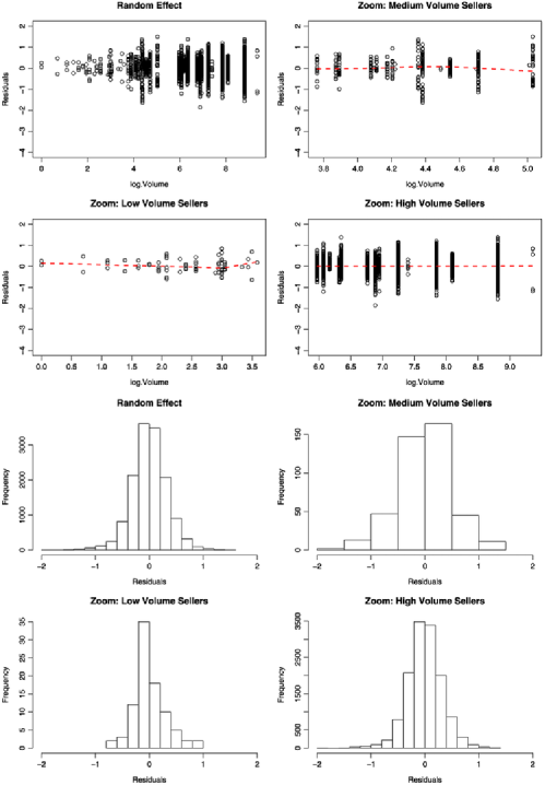
Figure 8: Residuals of the RE model.

Random effects models are often employed when there are repeat observations on the same subject or when the data is clustered [e.g., Agresti et al. (2000)]. Since we have many repeat auctions by the same seller, adding a random, seller-specific effect to the model in (9) lends itself as a natural remedy for OLS. While RE models have become popular only recently with the advent of powerful computing and efficient algorithms, WLS has been around for a longer time as a possible solution for heteroscedasticity [Greene (2003)]. While the principle of WLS is powerful, it assumes that the matrix of weights is known (or at least known up to a parameter value), which reduces its practical value. In our context, we use weights that are inversely proportional to the residual variance in each cluster. We will now compare both approaches and see if they result in more plausible models for e-loyalty.

Table 6 (second and third panels) shows the results of the RE and WLS models, respectively. We can see that WLS results in a very poor model fit (both in terms of $R$-squared and AIC). While the RE model results in much better model fit (compared to both the WLS and the OLS model), it is curious that seller feedback is insignificant, similar to the OLS model above. In fact, it is quite curious that none of the seller-related variables (feedback, loyalty or volume) are significant in the RE model. This finding suggests that none of the actions taken by the seller affect the outcome of an auction, which contradicts both common practitioner knowledge as well as previous research on the topic [Bajari and Hortacsu (2004); Ba and Pavlou (2002); Lucking-Reiley et al. (2007)].

Figure 8 shows the residuals of the RE model. We can see that the magnitude of the residuals has decreased, suggesting a better model fit. This is expected as the random effects account for seller-specific variation due to individual selling strategies (e.g., seller-specific auction parameters or product descriptions), which all may lead to differences in final price. But we can also see that the RE model still suffers from heteroscedasticity (much larger residual variance for high volume sellers compared to low volume sellers).

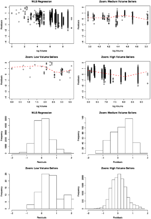
Figure 9: Residuals of the WLS model.

Figure 9 shows the corresponding residuals of the WLS approach. While we would have expected that WLS tames the heteroscedasticity somewhat, it appears that model fit has become worse. (This is also supported by the much poorer values of $R$-squared and AIC.) One possible reason is that weights have to be chosen by the user (inversely proportional to seller volume, in our case), which may not result in the most appropriate weighting of the data.

4.3 Data segmentation

None of the proposed modeling alternatives so far have lead to models with reasonable residuals or economically defendable conclusions. In fact, we have seen that the model fit differs systematically by the seller volume. We take this as evidence that the data may be segmented into different seller volume clusters. We have seen earlier (e.g., Figures 1 and 2) that sellers of different magnitude exhibit quite different effects on bidders. We will thus now first cluster the data and then model each data-segment separately.

We first cluster the data by seller volume (low, medium and high) and then apply OLS regression within each segment, resulting in three different regression models, one for each segment. We select the clusters with the objective of minimizing the residuals mean squared errors within each cluster. This results in the following three segments: Low volume sellers—40 transactions or less; medium volume sellers—40–350 transactions; high volume sellers—more than 350 transactions.

Figure 10 shows the residuals of the resulting three models. We can see that the model fit is much better compared to the previous modeling approaches. In each segment the magnitude of the residuals is very small, all residuals scatter around the origin, and we also no longer find evidence for heteroscedasticity in any of the three segments. In fact, the model fit statistics (see Table 7) suggest that the segmentation approach leads to a much better representation of the data compared to either OLS, RE or WLS models.

Table 7 shows the parameter estimates for each segment. We can see that the relationship between loyalty, trust and price varies from segment to segment. In fact, while for the low volume sellers the significance of all seller-related variables (feedback, loyalty or volume) is low, both feedback and volume are much more significant than loyalty. (Note the much smaller $p$-values of seller feedback and volume.) This suggests that while seller-related actions may not play much of a role for low volume sellers (such as rookie sellers and sellers that are new to the market), trust is much more important compared to loyalty. This makes sense as low volume sellers have not much of a chance to establish a loyal customer base due to the infrequency of their transactions.

This is different for medium volume sellers. For medium volume sellers, loyalty and volume are more significant than feedback. This suggests that with increasing frequency of transactions, repeat transactions (i.e., loyalty) have a more dominant effect on a seller’s bottom line. This effect is even more pronounced for high volume sellers. This suggests that high volume sellers are most affected by the actions of repeat customers. It is also interesting that both feedback and loyalty are significant for high volume sellers. This suggests that in the presence of two sellers with the same reputation, buyers “act with memory” and return to repeat their previous shopping experience.

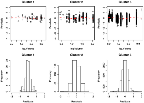
Figure 10: Residuals after data segmentation. The left panel shows the residuals of an OLS model fitted only to the data from cluster 1 (low volume sellers); the middle and right panels show the corresponding residuals for medium and high volume sellers.

In order to precisely quantify the effect of loyalty in each segment, consider Table 8. In that table, we present, for each of the 5 theoretical loyalty distributions from Figure 6, their corresponding combined effect on the regression model. That is, we compute the combined effect of PC1 and PC2, holding all other variables in the model constant.

=300pt Coefficient Estimate Std. error $\bolds p$-value (Intercept) $-0.51$ 0.36 0.16 Auction duration $0.04$ 0.02 0.10 log(item quantity $+$ 1) $-0.06$ 0.10 0.50 Bid count $0.12$ 0.01 0.00 log(Pieces) $0.15$ 0.06 0.02 Size $0.06$ 0.03 0.05 log(seller feedback $+$ 1) $0.08$ 0.04 0.07 Loyalty-PC1 $-0.22$ 0.16 0.18 Loyalty-PC2 $-0.03$ 0.13 0.82 log(Volume) $-0.10$ 0.06 0.07 AIC 63 $R$-squared $0.76$ (Intercept) $-0.49$ 0.38 0.20 Auction duration $-0.05$ 0.01 0.00 log(item quantity $+$ 1) $-0.11$ 0.19 0.58 Bid count $0.17$ 0.01 0.00 log(Pieces) $0.03$ 0.01 0.05 Size $0.01$ 0.01 0.58 log(seller feedback $+$ 1) $-0.01$ 0.02 0.65 Loyalty-PC1 $-0.24$ 0.12 0.04 Loyalty-PC2 $0.28$ 0.19 0.15 log(Volume) $0.33$ 0.08 0.00 AIC 534 $R$-squared $0.75$ (Intercept) $1.68$ 0.10 0.00 Auction duration $0.02$ 0.00 0.00 log(item quantity $+$ 1) $-0.25$ 0.04 0.00 Bid count $0.05$ 0.00 0.00 log(Pieces) $0.39$ 0.00 0.00 Size $0.06$ 0.00 0.00 log(seller feedback $+$ 1) $0.42$ 0.01 0.00 Loyalty-PC1 $7.39$ 0.16 0.00 Loyalty-PC2 $-9.41$ 0.17 0.00 log(Volume) $-0.78$ 0.02 0.00 AIC 10,482 $R$-squared $0.83$

Table 7: Regression models on three data segments. The top panel shows the result for the low volume sellers; middle panel shows medium volume sellers; bottom panel shows high volume sellers. The response is always log-price

Table 8: Quantifying the effect of the 5 theoretic loyalty distributions from Figure 6

	Pure lyty	Strong lyty	Somewhat loyal	Two extremes	Pure dislyty
Cluster 1 (low)	$-0.14$	$-0.12$	$-0.07$	$0.00$	$0.14$
Cluster 2 (medium)	$0.07$	$0.03$	$-0.10$	$0.11$	$0.15$
Cluster 3 (high)	$-2.60$	$-1.29$	$3.14$	$-3.61$	$-4.62$

We can see that in clusters 1 and 2, the effect of loyalty is considerably small, consistent with the small (and insignificant) coefficients for low and medium volume sellers in Table 7. For cluster 3, it is interesting that only the distribution corresponding to somewhat loyal buyers results in a positive price effect. In fact, we can see that extreme loyalty (i.e., the distributions for both pure loyalty and pure disloyalty) has negative implications for a seller’s bottom line. While the effect of disloyal bidders is easier to explain (disloyal bidders may “shop around” more actively in the search for lower prices and, as a result, drive down a seller’s revenue), the negative effect of purely loyal bidders may be due to the fact that a bidder who exclusively interacts with the same seller may form an opinion about that seller’s “going price” which results in a less competitive auction process (and thus renders the transaction into a fixed-price transaction). Thus, our results show that the effect of loyalty is surprisingly “nonlinear” in that a mix of somewhat loyal bidders results in the most competitive auction environment and thus the highest price for the seller.

Another way of quantifying the impact of loyalty is via the difference between pure loyalty and pure disloyalty. Notice that the difference in estimated coefficients equals ($-2.60-4.62)\approx$ 2, which (as the response is on the log-scale) implies that, all else equal, sellers with a purely loyal customer base extract price premiums 200% higher compared to sellers with a purely disloyal customer base.

5 Conclusion

In this paper we investigate loyalty of online transactions. Loyalty is an important element to many business models, and it is especially difficult to manage in the online domain where consumers are offered different choices that are often only a mouse-click away. We study loyalty in online auctions. We derive online loyalty from the network of sellers and bidders and find that while bidder’s loyalty can have a strong impact on the outcome of an auction, the magnitude of its impact varies depending on the size of the seller.

We want to point out that while we find that loyalty has a strong effect on price, we do not determine the cause of loyalty. A buyer’s loyalty can have many different causes such as a high-quality product, a speedy delivery, or an otherwise seamless service. While loyalty could also be caused by price itself (i.e., a buyer returning to the same seller because of a low price), it is unlikely in our setting due to the auction process. Recall that in an auction the price is not fixed. Thus, a seller offering a top notch product and an outstanding service will sooner or later see an increase in bidders and, as a result, more competition and thus a higher price for her product. Thus, loyalty is unlikely to be caused merely by bargain sellers.

Also, we want to emphasize that while we find many repeat transactions between the same seller–bidder pair in our data, the frequency of these repeat interactions may depend on the type of product and the buyer’s demand for this product. In our case (beads, i.e., arts and crafts), buyers have frequently re-occurring demand for the same product and, hence, the chances that a buyer will seek out the same seller rise drastically. On the other hand, if we were to consider the market for a product in which repeat transactions are less common (such as computers, digital cameras, automobiles, etc.), our loyalty networks would likely not be as dense. Nevertheless, it would be equally important for sellers to understand what factors drive consumers to spend money and we believe that loyalty networks are one way to address that question.

There are several statistical challenges when studying loyalty networks. First, deriving quality measures from the observed networks requires a method that can capture both the intensity as well as the size of loyalty. We accomplish this using ideas from functional data analysis. Second, modeling the effect of loyalty is complicated by the extreme skew of loyalty networks. Our analysis shows that many different approaches can lead to model misspecification and, as a consequence, to economically wrong conclusions. Similar problems likely exist in other studies on online markets (e.g., those that study seller feedback or reputation where one also records repeat observations on the same seller). Our analysis leads us to conclude that the data is too segmented to be treated by a single model and thus propose a data-clustering approach.

Another statistical challenge revolves around sampling bidder–seller networks. As pointed out earlier, we have the complete set of bidding records for a certain product (Swarovski beads, in this case) for a certain period of time (6 months). As a result, we have the complete bidder–seller network for this product, for this time frame. While sampling would be an alternative, it would result in an incomplete network (since we would no longer observe all nodes/arcs). As a result, we would no longer be able to compute loyalty without error, which would bring up an interesting statistical problem. But we caution that sampling would have to be done very carefully. While one could, at least in theory, sample randomly across all different eBay categories, it would bring up several problems. The biggest problem is that we would now be attempting to compare loyalty across different product types. For instance, we would be comparing, say, a bidder’s loyalty for purchasing beads (a very low price, low stake item) with that of purchasing digital cameras, computers, or even automobiles (all of which are high price and high stakes), which would be conceptually very questionable.

We also want to mention that we treat the bidder–seller network as static over time. Our data spans a time-frame of only 6 months and we assume that loyalty is static over this time-frame. This assumption is not too unrealistic as many marketing models consider loyalty to be static over much longer time frames [Fader and Hardie (2006); Fader, Hardie and Lee (2006); Donkers, Verhoef and De Jong (2003)]. While incorporating a temporal dimension (e.g., by using a network with a sliding window or via down-weighting older interactions) would be an intriguing statistical challenge, it is not quite clear how to choose the width of the window or the size of the weights. Moreover, we also explicitly tested for learning effects by buyers over time and could not find any strong statistical evidence for it.

And finally, in this work we address one specific kind of network dependence, namely, that between buyers and sellers. We argue that the lack of independence among observations on the same sellers leads to a clustering-effect and we investigate several remedies to this challenge. However, the dependence structure may in fact be far more complex. As bidders are linked to sellers which, in turn, are linked again to other bidders, the true dependence structure among the observations may be far more complex. This may call for innovative statistical methodology and we hope to have sparked some new ideas with our work.

References

- Agresti et al. (2000) Agresti, A., Booth, J., Hobert, J. and Caffo, C. (2000). Random effects modeling of categorical response data. Sociological Methodology 30 27–80.
- Ba and Pavlou (2002) Ba, S. and Pavlou, P. (2002). Evidence of the effect of trust building technology in electronic markets: Price premiums and buyer behavior. MIS Quarterly 26 243–268.
- Bailey et al. (2008) Bailey, J., Gao, G., Jank, W., Lin, M., Lucas, H. C. and Viswanathan, S. (2008). The long tail is longer than you think: The surprisingly large extent of online sales by small volume sellers. Technical report, RH Smith School of Business, University of Maryland. Available at SSRN: http://ssrn.com/abstract=1132723.
- Bajari and Hortacsu (2004) Bajari, P. and Hortacsu, A. (2004). Economic insights from internet auctions. Journal of Economic Literature 42 457–486.
- Bapna, Jank and Shmueli (2008) Bapna, R., Jank, W. and Shmueli, G. (2008). Consumer surplus in online auctions. Inform. Syst. Res. 19 400–416.
- Brown and Morgan (2006) Brown, J. and Morgan, J. (2006). Reputation in online auctions: The market for trust. California Management Review 49 61–81.
- Donkers, Verhoef and De Jong (2003) Donkers, B., Verhoef, P. C. and De Jong, M. (2003). Predicting customer lifetime value in multi-service industries. Technical report, ERIM Report Series Reference No. ERS-2003-038-MKT. Available at SSRN: http://ssrn.com/abstract=411666.
- Fader and Hardie (2006) Fader, P. and Hardie, B. (2006). How to project customer retention. Technical report. Available at SSRN: http://ssrn.com/abstract=801145.
- Fader, Hardie and Lee (2006) Fader, P., Hardie, B. and Lee, K. L. (2006). CLV: More than meets the eye. Technical report, Available at SSRN: http://ssrn.com/abstract=913338.
- Greene (2003) Greene, W. H. (2003). Econometric Analysis, 4th ed. Prentice Hall, Upper Saddle River, NJ.
- Haruvy et al. (2008) Haruvy, E., Popkowski Leszczyc, P., Carare, O., Cox, J., Greenleaf, E., Jap, S., Jank, W., Park, Y. and Rothkopf, M. (2008). Competition between auctions. Marketing Letters 19 431–448.
- Jank and Shmueli (2007) Jank, W. and Shmueli, G. (2007). Modeling concurrency of events in online auctions via spatio-temporal semiparametric models. J. Roy. Statist. Soc. Ser. C 56 1–27. \MR2339160
- Jank and Zhang (2008) Jank, W. and Zhang, S. (2008). An automated and data-driven bidding strategy for online auctions. Technical report, RH Smith School of Business, Univ. Maryland. Available at SSRN: http://ssrn.com/abstract=1427212.
- Kneip and Utikal (2001) Kneip, A. and Utikal, K. J. (2001). Inference for density families using functional principal component analysis. J. Amer. Statist. Assoc. 96 519–542. \MR1946423
- Lingfang (2006) Lingfang, L. (2006). Reputation, trust and rebates: How online auction markets can improve their feedback systems. Journal of Economics and Management Strategies. To appear.
- Livingston (2005) Livingston, J. (2005). How valuable is a good reputation? A sample selection model of internet auctions. Rev. Econ. Statist. 87 453–465.
- Lucking-Reiley et al. (2007) Lucking-Reiley, D., Bryan, D., Prasad, N. and Reeves, D. (2007). Pennies from Ebay: The determinants of price in online auctions. The Journal of Industrial Economics 55 223–233.
- Ramsay and Silverman (2005) Ramsay, J. and Silverman, B. (2005). Functional Data Analysis. Springer, New York. \MR2168993
- Reddy and Dass (2006) Reddy, S. K. and Dass, M. (2006). Modeling online art auction dynamics using functional data analysis. Statist. Sci. 21 179–193. \MR2324077