Stability of gravity-scalar systems for domain-wall models with a soft wall

Abstract

We show that it is possible to create an RS soft-wall model, a model with a compact extra dimension, without using fundamental branes. All that is required are bulk scalar fields minimally coupled to gravity. Of crucial importance is the stability of the size of the extra dimension. Without branes, one cannot easily implement the Goldberger-Wise mechanism, and instead it must be shown that the scalar configuration is stable in its own right. We use the superpotential approach for generating solutions, the so called ’fake supergravity’ scenario, and show that configurations generated in such a way are always free of tachyonic modes. Furthermore, we show that the model is also free of zero modes (in the spin-0 sector) if all the scalars have odd parity. We discuss the hierarchy problem in soft-wall models, and applications of our analysis to the AdS/QCD correspondence.

NIKHEF/2010-035

1 Introduction

Extra dimensions are a plausible extension to the standard model of particle physics. In particular, much attention has been given to the type I Randall-Sundrum (RS) model [1], where the electroweak hierarchy can be naturally generated by the warping of a compact extra dimension. In their original realisation, these models have fundamental branes of negative tension, or hard-walls, at the boundary of the extra dimension. Recently there has been interest in a new type of RS-like warped spacetime: a compact spacetime where the negative tension brane is replaced with a physical singularity. These soft-wall models were originally designed to yield linear Regge trajectories in the context of the AdS/CFT correspondence [2], but have since been the basis of actual models beyond the standard model [3, 4, 5, 6, 7, 8, 9, 10], and also provide a holographic dual description of unparticle models [11, 12].

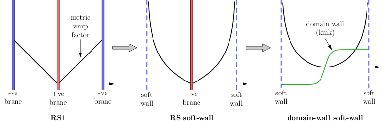
Our aim is take the soft-wall model and go one step further by removing the final, positive-tension brane at the origin, and replacing it with a suitable scalar field profile, such as a domain wall. Such a model will then describe a compact extra dimension without the use of fundamental dynamical branes. This is interesting because it is a purely field theoretical construction and requires no appeal to string theory. Figure 1 depicts the progression from RS1 models to domain-wall soft-wall models. In what follows, we analyse the stability of such domain-wall models, and show that they are capable of solve the hierarchy problem. See reference [13] for details.

Figure 1: From RS1 to RS soft-wall to domain-wall soft-wall. The domain-wall set-up provides a purely field theoretic construction of a compact extra dimension.

2 Warped Background Configuration

We work in the framework of 5D general relativity, with $N$ scalar fields $\Phi_{i}$ minimally coupled to gravity. We also allow the presence of brane terms for completeness. The action for such a set-up is given by

$$\mathcal{S}=\int d^{4}x\,dy\left[\sqrt{-g}\left(M^{3}R+\mathcal{L}_{\text{matter}}\right)-\sqrt{-g_{4}}\lambda\right]\>,$$ (1)

where $M$ is the 5D Planck mass and the matter and brane terms are

$$\mathcal{L}_{\text{matter}} =-\frac{1}{2}\sum_{i=1}^{N}g^{PQ}\partial_{P}\Phi_{i}\partial_{Q}\Phi_{i}-V(\{\Phi_{i}\})\>,$$ (2)

$$\lambda =\lambda(\{\Phi_{i}\})=\sum_{\alpha}\lambda_{\alpha}(\{\Phi_{i}\})\delta(y-y_{\alpha})\>.$$ (3)

Here, $V(\{\Phi_{i}\})$ is the scalar potential and $\lambda_{\alpha}(\{\Phi_{i}\})$ the brane localised potential (including brane tension) for the brane at $y_{\alpha}$. Our aim is to study the general stability conditions for non-trivial background configurations of this class of models.

We specialise to backgrounds that depend only on the extra dimension $y$, and denote the scalar background solutions $\phi_{i}(y)$. The RS background metric ansatz is

$$ds^{2}=e^{-2\sigma(y)}\eta_{\mu\nu}dx^{\mu}dx^{\nu}+dy^{2}\>,$$ (4)

where $\mu,\nu$ index the 4D subspace. Einstein’s equations are $G_{MN}=\frac{1}{2M^{3}}T_{MN}$ and yield, together with the Euler-Lagrange equations,

$$6M^{3}\sigma^{\prime\prime}=\sum_{i}\phi_{i}^{\prime 2}+\lambda(\{\phi_{j}\})\>,$$ (5)

$$6M^{3}\left(4\sigma^{\prime 2}-\sigma^{\prime\prime}\right)=-2V\left(\{\phi_{j}\}\right)-\lambda\left(\{\phi_{j}\}\right)\>,$$ (6)

$$\phi_{i}^{\prime\prime}-4\sigma^{\prime}\phi_{i}^{\prime}-V_{i}(\{\phi_{j}\})-\lambda_{i}(\{\phi_{j}\})=0\>.$$ (7)

The notation $V(\{\phi_{i}\})$ means that the potential is to be evaluated with the background fields $\phi_{i}$. A subscript $i$ on $V$ or $\lambda$ denotes partial differentiation with respect to the field $\Phi_{i}$.

Given a particular $V$ and $\lambda$, the space of background configurations is parameterised by the integration constants of the system. For a particular choice of integration constants, that is, a particular background, we want to know if such a choice is stable within the space of configurations. We shall study local, perturbative stability by adding small fluctuations to the background, turning the problem into an eigenvalue problem. For the initial stages our analysis will be for an arbitrary scalar potential $V$. Later on we will need to specialise to the fake supergravity approach.

3 Perturbations

The general ansatz which takes into account both spin-0 and spin-2 perturbations is

$$ds^{2}=e^{-2\sigma(y)}\left[(1-2F(x^{\mu},y)\eta_{\mu\nu}+h_{\mu\nu}(x^{\mu},y)\right]dx^{\mu}dx^{\nu}+\left[1+G(x^{\mu},y)\right]^{2}dy^{2}\>,$$ (8)

$$\Phi_{i}(x^{\mu},y)=\phi_{i}(y)+\varphi_{i}(x^{\mu},y)\>.$$ (9)

Here we work in the axial gauge, $h_{\mu 5}=0$, with transverse traceless part $\partial^{\mu}h_{\mu\nu}=\eta^{\mu\nu}h_{\mu\nu}=0$. The $(ij)$ Einstein’s equations (off-diagonal spatial) enforce $G=2F$ which we take from now on. The rest of Einstein’s equations correspond to $(\mu\nu)$, $(\mu 5)$ and $(55)$, and taking the 4-trace of the $(\mu\nu)$ equations shows that the spin-2 and spin-0 perturbations decouple from one another.

3.1 Spin-2 Perturbations

The spin-2 perturbation $h_{\mu\nu}$ decouples from $F$ and $\varphi_{i}$. The equation for $h_{\mu\nu}$ is

$$-e^{2\sigma}\Box h_{\mu\nu}-h_{\mu\nu}^{\prime\prime}+4\sigma^{\prime}h_{\mu\nu}^{\prime}=0\>.$$ (10)

There is always a zero mode, $h_{\mu\nu}^{\prime}=0$, which is normalisable. This is the well-known 4D massless graviton from the RS model [14]. In conformal coordinates $z$ defined by $dy=e^{-\sigma}\,dz$ with rescaled $h_{\mu\nu}=e^{3\sigma/2}\tilde{h}_{\mu\nu}$ we can write this equation as a Schrödinger-like equation in a self-adjoint form:

$$(\partial_{z}-\frac{3}{2}\sigma^{\prime})(-\partial_{z}-\frac{3}{2}\sigma^{\prime})\tilde{h}_{\mu\nu}=\Box\tilde{h}_{\mu\nu}\>.$$ (11)

Applying supersymmetric quantum mechanics we find that there are no tachyonic modes in the spin-2 sector. Thus the spin-2 fluctuations do not destabilise the configuration.

3.2 Spin-0 Perturbations

The spin-0 sector is significantly more complicated than the spin-2 sector, since physical modes are mixtures of $F$ and $\varphi_{i}$. The equations for these perturbations consist of two of Einstein’s equations and the Euler-Lagrange equations (sum over repeated scalar indices):

$$6M^{3}(F^{\prime}-2\sigma^{\prime}F)=\phi_{i}^{\prime}\varphi_{i}\>,$$ (12)

$$6M^{3}(-e^{2\sigma}\Box F-2\sigma^{\prime}F^{\prime}+F^{\prime\prime})=2\phi_{i}^{\prime}\varphi_{i}^{\prime}+2\left.\lambda\right|_{\text{bg}}F+\left.\lambda_{i}\right|_{\text{bg}}\varphi_{i}\>.$$ (13)

$$e^{2\sigma}\Box\varphi_{i}+\varphi_{i}^{\prime\prime}-4\sigma^{\prime}\varphi_{i}^{\prime}-6F^{\prime}\phi_{i}^{\prime}-\left.(4V_{i}+2\lambda_{i})\right|_{\text{bg}}F-\left.(V_{ij}+\lambda_{ij})\right|_{\text{bg}}\varphi_{j}=0\>.$$ (14)

To simplify these equations we go to conformal coordinates $z$ as above and rescale the fields by $F=e^{3\sigma/2}\chi(z)/\sqrt{12}$ and $\varphi_{i}=M^{3/2}e^{3\sigma/2}\psi_{i}(z)$. Equations (12) through (14) then become a set of coupled Schrödinger-like equations:

$$-\chi^{\prime\prime}+(\mathcal{V}_{00}+\mathcal{B}_{00})\chi+(\mathcal{V}_{0i}+\mathcal{B}_{0i})\psi_{i} =\Box\chi\>,$$ (15)

$$-\psi_{i}^{\prime\prime}+(\mathcal{V}_{ij}+\mathcal{B}_{ij})\psi_{j}+(\mathcal{V}_{0i}+\mathcal{B}_{0i})\chi =\Box\psi_{i}\>,$$

where the effective potential $\mathcal{V}$ has components

$$\mathcal{V}_{00}=\frac{9}{4}\sigma^{\prime 2}+\frac{5}{2}\sigma^{\prime\prime}\>,\quad\mathcal{V}_{0i}=\frac{2\phi_{i}^{\prime\prime}}{\sqrt{3M^{3}}}\>,\quad\mathcal{V}_{ij}=\left(\frac{9}{4}\sigma^{\prime 2}-\frac{3}{2}\sigma^{\prime\prime}\right)\delta_{ij}+\frac{\phi_{i}^{\prime}\phi_{j}^{\prime}}{M^{3}}+e^{-2\sigma}\left.V_{ij}\right|_{\text{bg}}\>,$$ (16)

and the brane terms are

$$\mathcal{B}_{00}=\frac{1}{3M^{3}}e^{-2\sigma}\left.\lambda\right|_{\text{bg}}\>,\qquad\mathcal{B}_{0i}=\frac{1}{\sqrt{3M^{3}}}e^{-2\sigma}\left.\lambda_{i}\right|_{\text{bg}}\>,\qquad\mathcal{B}_{ij}=e^{-2\sigma}\left.\lambda_{ij}\right|_{\text{bg}}\>.$$ (17)

Equation (15) defines the physical spin-0 spectrum. The symmetry of the cross-coupling ensures that the eigenvalues of this spectrum are real. To demonstrate stability of a given background configuration, we must also show that all eigenvalues are positive.

4 Fake supergravity

Our aim is to find a class of models which have strictly positive eigenvalues in the spin-0 sector, ensuring the stability of the background configuration. We specialise to the case without brane terms ($\lambda=0$) and where the scalar potential is generated from a superpotential $W(\{\Phi_{i}\})$ using the fake supergravity approach [15, 16]

$$V(\{\Phi_{i}\})=\sum_{i}\frac{1}{2}\left[W_{i}(\{\Phi_{i}\})\right]^{2}-\frac{1}{3M^{3}}\left[W(\{\Phi_{i}\})\right]^{2}\>,$$ (18)

where $W_{i}\equiv dW/d\Phi_{i}$. For such a potential, equations (5) through (7) simplify to

$$\sigma^{\prime}(y)=W(\{\phi_{i}\})/6M^{3}\>,\qquad\phi_{i}^{\prime}(y)=W_{i}(\{\phi_{i}\})\>.$$ (19)

This is a set of first order equations; $W$ encodes for both $V$ and some of the integration constants. Without loss of generality we can take $\sigma(y_{0})=0$, leaving $N$ integration constants for the boundary values of $\phi_{i}$. So, given a particular $W$, the set $\{\phi_{i}(y_{0})\}$ will then uniquely define a configuration. We want to know if such a configuration is stable.

Using the fake supergravity approach, one can write the spin-0 effective potential as $\mathcal{V}=S^{2}+S^{\prime}$ where

$$S=e^{-\sigma}\left.\begin{pmatrix}\tfrac{1}{12M^{3}}W&\,\,\tfrac{1}{\sqrt{3M^{3}}}W_{j}\\ \tfrac{1}{\sqrt{3M^{3}}}W_{i}&\,\,\tfrac{-1}{4M^{3}}\delta_{ij}W+W_{ij}\end{pmatrix}\right|_{\text{bg}}\>.$$ (20)

Then equation (15) takes the self-adjoint form

$$(\partial_{z}+S^{\dagger})(-\partial_{z}+S)\Psi=\Box\Psi\>,$$ (21)

where $\Psi=(\chi,\psi_{i})$. For a warped metric the relevant boundary terms vanish and supersymmetric quantum mechanics tells us that the eigenvalues of the spin-0 sector are non-negative. The background is thus free of tachyonic modes. To ensure complete stability, we must still analyse the existence of zero mode solutions. Such zero modes can, for example, correspond to changes in the size of the compact extra dimension, rendering the set-up unstable.

4.1 Zero modes with $N=1$

With $N=1$ scalar we can use the Einstein constraint equation to eliminate $\psi_{1}$ in terms of $\chi$. Then let $\chi=S_{01}g$, with $S_{01}$ defined by equation (20). The Schrödinger-like equation for $g$ is

$$(\partial_{z}-S_{11})(-\partial_{z}-S_{11})g+S_{01}^{2}g=\Box g\>.$$ (22)

Multiplying this equation from the left by $g^{*}$ and integrating over the extra dimension yields

$$\int\left|(-\partial_{z}-S_{11})g\right|^{2}dz+\int\left|S_{01}g\right|^{2}+\text{(boundary terms)}=\Box\int|g|^{2}dz\>.$$ (23)

For a warped metric the boundary terms vanish, and the existence of a zero mode with $\Box g=0$ requires both $(-\partial_{z}-S_{11})g=0$ and $S_{01}g=0$. Thus $g=0$ and we can conclude that systems with $N=1$ scalar using the fake supergravity approach do not have a zero mode.

4.2 Zero modes with $N\geq 2$

Set-ups with more than one scalar field can in general posses a zero mode. Nevertheless, we can formulate a simple criterion that can be used to find models which do not have a zero mode: for a system of definite parity, the number of independent normalisable zero modes is at most equal to the number of even scalar fields. This is essentially a statement about integration constants. In the fake supergravity approach, the background configuration is given by the solutions to the first order equations (19). The restriction to models with parity eliminates those integration constants associated with odd-parity scalars, since their field value must vanish at $y=0$. Unique solutions to the fake supergravity equations are then parameterised by the integration constants of the even-parity fields. The final point is that zero modes move us continuously through this space of solutions, so there cannot be more zero modes than the number of even fields.

5 Applications

We shall look at two example models with $N=2$ scalar fields to illustrate the above criterion about the existence of zero modes. The second model is an example of a stable domain-wall soft-wall set-up. Following this we make some comments about AdS/QCD.

5.1 Example 1 — unstable even system

Consider the superpotential

$$W\left(\Phi_{1},\Phi_{2}\right)=e^{\nu\Phi_{1}}\left(a\,\Phi_{2}-b\,\Phi_{2}^{3}\right)\>,$$ (24)

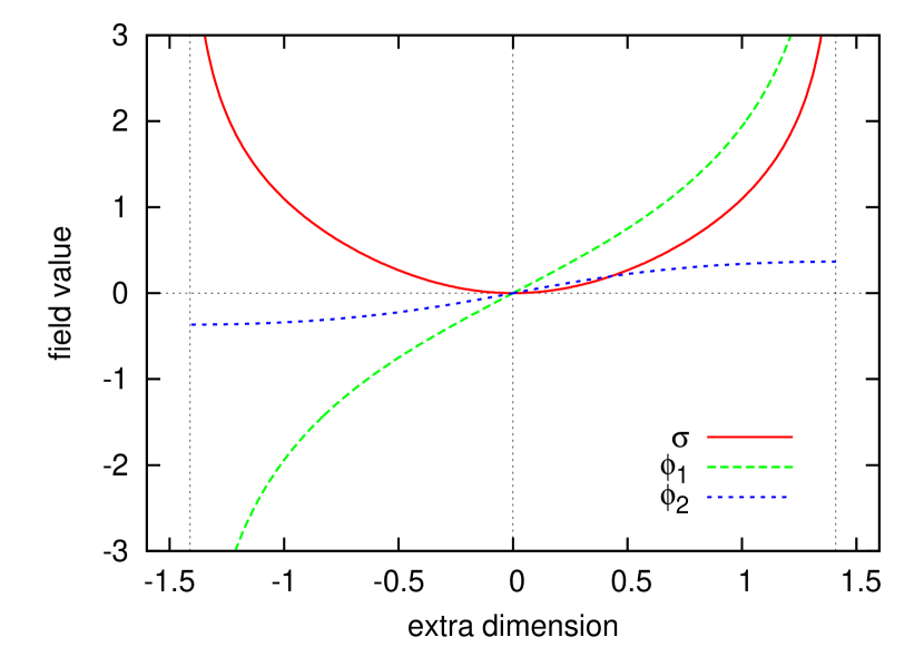
where $\Phi_{1}$ and $\Phi_{2}$ are the dilaton and kink fields respectively. We choose $\Phi_{1}$ to have even and $\Phi_{2}$ to have odd parity in $y$. See Figure 3 for representative background solutions (the plots use units where $6M^{3}=1$). In these solutions there is a choice of integration constant for $\Phi_{1}$ and our criterion tells us that a corresponding spin-0 zero mode can exist. Such a mode in fact does exist, and is given by $(\chi,\psi_{1},\psi_{2})=N(-\nu,\sqrt{2},0)e^{-3\sigma/2}\eta(x^{\mu})$ where $N$ is a normalisation constant and $\eta$ is the 4D mode. This zero mode physically corresponds to changes in the size of the extra dimension, so the background configuration is not stable.

Figure 2: Background solutions for Example 1. Parameters are $\nu=1.4$, $a=0.5$, $b=0.3$. The size of the extra dimension is not stabilised and depends on the value $\phi_{1}(0)$.

Figure 3: Background solutions for Example 2. Parameters are $\alpha=1$, $\nu=1.4$, $a=0.5$, $b=0.3$. The configuration is stable and is an example of a domain-wall soft-wall model.

5.2 Example 2 — stable odd system

The second model has the superpotential

$$W\left(\Phi_{1},\Phi_{2}\right)=\alpha\,\sinh(\nu\,\Phi_{1})+\left(a\,\Phi_{2}-b\,\Phi_{2}^{3}\right)\>,$$ (25)

where $\Phi_{1}$ and $\Phi_{2}$ are now both taken to have odd parity. As a consequence of this parity choice, there are no integration constants to choose, and, by our criterion, there cannot exist any zero modes. The background solution is unique and stabilised, and the size of the extra dimension is fixed by the parameters in $W$; see Figure 3. The field $\Phi_{2}$ is in a kink configuration and replaces the brane in usual RS soft-wall models, providing an example of a domain-wall model with a soft wall. Figure 4 shows how the electroweak hierarchy can be generated in such a model.

Figure 4: Solving the hierarchy problem using the domain-wall soft-wall model of Example 2. The size of the compact extra dimension in conformal coordinates, $z_{\text{size}}$, sets the characteristic mass scale. Bulk fields have a KK mass scale $m_{\text{KK}}\sim z_{\text{size}}^{-1}$ and the hierarchy problem is solved if $z_{\text{size}}\sim 10^{16}$ can be obtained for $\mathcal{O}(1)$ model parameters. The plot has $a=b=1$ in equation (25) and shows $z_{\text{size}}$ versus $\alpha$ for $\nu=1.0\ldots 1.4$. To obtain the relevant hierarchy one should take $\alpha\simeq 0.02$ and $\nu\simeq 1.0$.

5.3 Application to AdS/QCD

Soft-wall models were originally motivated by attempts to construct 5D AdS models of QCD [2]. Having a soft wall in the infrared (large $y$) yields linear Regge trajectories; the meson excitations in the QCD dual theory have masses which scale like $m_{n}^{2}\sim n$, where $n$ is the excitation number. Scalar fluctuations in the AdS picture correspond to glueball and scalar meson excitations in the dual QCD theory. Since the fake supergravity approach is common in the literature, and it seems that more than one scalar is required to dynamically generate the background (see for example [3]), our Schrödinger-like equation for the spin-0 eigenvalues, equations (20) and (21), can be used to compute the scalar spectrum with multiple background fields.

This research was done in collaboration with S. M. Aybat. It was supported by the Netherlands Foundation for Fundamental Research of Matter (FOM) and the National Organisation for Scientific Research (NWO).

References

- [1] Randall L and Sundrum R 1999 Phys. Rev. Lett. 83 3370–3373 (Preprint hep-ph/9905221)
- [2] Karch A, Katz E, Son D T and Stephanov M A 2006 Phys. Rev. D74 015005 (Preprint hep-ph/0602229)
- [3] Batell B and Gherghetta T 2008 Phys. Rev. D78 026002 (Preprint 0801.4383)
- [4] Falkowski A and Perez-Victoria M 2008 JHEP 12 107 (Preprint 0806.1737)
- [5] Batell B, Gherghetta T and Sword D 2008 Phys. Rev. D78 116011 (Preprint 0808.3977)
- [6] Delgado A and Diego D 2009 Phys. Rev. D80 024030 (Preprint 0905.1095)
- [7] Mert Aybat S and Santiago J 2009 Phys. Rev. D80 035005 (Preprint 0905.3032)
- [8] Gherghetta T and Sword D 2009 Phys. Rev. D80 065015 (Preprint 0907.3523)
- [9] Cabrer J A, von Gersdorff G and Quiros M 2009 (Preprint 0907.5361)
- [10] von Gersdorff G 2010 (Preprint 1005.5134)
- [11] Cacciapaglia G, Marandella G and Terning J 2009 JHEP 02 049 (Preprint 0804.0424)
- [12] Falkowski A and Perez-Victoria M 2009 Phys. Rev. D79 035005 (Preprint 0810.4940)
- [13] Aybat S M and George D P 2010 JHEP 09 010 (Preprint 1006.2827)
- [14] Randall L and Sundrum R 1999 Phys. Rev. Lett. 83 4690–4693 (Preprint hep-th/9906064)
- [15] DeWolfe O, Freedman D Z, Gubser S S and Karch A 2000 Phys. Rev. D62 046008 (Preprint hep-th/9909134)
- [16] Freedman D Z, Nunez C, Schnabl M and Skenderis K 2004 Phys. Rev. D69 104027 (Preprint hep-th/0312055)