Correlations probed in direct two-nucleon removal reactions

Abstract

Final-state-exclusive momentum distributions of fast, forward travelling residual nuclei, following two nucleon removal from fast secondary radioactive beams of projectile nuclei, can and have now been measured. Assuming that the most important reaction mechanism is the sudden direct removal of a pair of nucleons from a set of relatively simple, active shell-model orbital configurations, such distributions were predicted to depend strongly on the total angular momentum $I$ carried by the two nucleons – the final state spin for spin $0^{+}$ projectiles. The sensitivity of these now-accessible observables to specific details of the (correlated) two-nucleon wave functions is of importance. We clarify that it is the total orbital angular momentum $L$ of the two nucleons that is the primary factor in determining the shapes and widths of the calculated momentum distributions. It follows that, with accurate measurements, this dependence upon the $L$ make-up of the two-nucleon wave functions could be used to assess the accuracy of (shell- or many-body) model predictions of these two-nucleon configurations. By use of several tailored examples, with specific combinations of active two-nucleon orbitals, we demonstrate that more subtle structure aspects may be observed, allowing such reactions to probe and/or confirm the details of theoretical model wave functions.

I Introduction

The momentum distributions of the residual nuclei, following the removal of a single nucleon from a fast radioactive secondary beam, offer sensitive probes of both strongly-bound and weakly-bound single-particle structure near the (asymmetric) Fermi surfaces of neutron-rich and neutron-deficient nuclei. Specifically, the shapes and widths of the exclusive residue momentum distributions were shown to be characteristic of the orbital angular momentum of the removed nucleon Han96 ; BaV98 ; HaT03 ; BeH04 ; Gad08 .

The simplest generalization to the case of direct two-nucleon removal is to describe the wave function of the two nucleons in the projectile by a product of nucleon wave functions in assumed single-particle orbitals. Doing so, the two nucleons are uncorrelated, other than both being bound to the same core BBC03 ; jatrnb7 . The heavy residue longitudinal momentum distributions in this limit, being essentially the convolution of those of the single-nucleons, depend on the assumed quantum numbers of the two nucleons, but, in the absence of explicit antisymmetrization or total angular momentum coupling of the two nucleons, are not characteristic of specific residue final states jatrnb7 .

More recent theoretical developments now treat fully the shell-model correlations of the two removed nucleons in the projectile many-body wave function TPB04 ; ToB06 . In the fully-correlated models the product of nucleonic wave functions is replaced by the shell-model two-nucleon overlap, incorporating (i) the two-nucleon parentage coefficients with respect to each residue final state (the two nucleon amplitudes, or TNA), (ii) proper antisymmetrization of the two removed nucleons, and (iii) proper angular momentum coupling.

The resulting theoretical description, and the insights developed here, are equally valid for reactions that remove two loosely- or strongly- bound nucleons. However, as has been discussed elsewhere TPB04 , in the case of removal of two loosely-bound nucleons the direct removal cross sections, of interest here, will be overwhelmed (experimentally) by indirect reaction (one-nucleon removal plus evaporation) events. See for example reference SiT09 for a quantitative consideration of the direct and indirect two-neutron removal reaction contributions along the neutron-rich carbon isotopic chain. For these reasons we will restrict our attention to examples for which the removed nucleons are strongly-bound, where the indirect removal paths are effectively closed, and for which the direct cross sections are accessible experimentally.

Demonstrative test cases, e.g. in Ref. STB09b , assumed the two nucleons originated from a single orbital – a pure configuration. In this limit the TNA enter only as a multiplicative (spectroscopic-like) factor and thus the new and interesting characteristics of the residue momentum distribution are a result of the correlations due to antisymmetrization and angular momentum coupling.

These developments demonstrate the potential of two-nucleon removal for exotic nucleus spectroscopy, showing the final-state-exclusive residue nucleus momentum distributions to have shapes and widths that are characteristic of the total angular momentum, $I$, carried by the removed pair of nucleons – and permitting final state spin assignments to be made STB09a . For the spin $J_{i}=0^{+}$ projectile nucleus examples used in Ref. STB09b , there was a high sensitivity of the residue momentum distributions to the final state total angular momentum $J_{f}=I$. Moreover, the shapes of these calculated distributions were robust with respect to variations of other key structure and reaction parameters, such as the nucleon separation energy. Further, the consideration of pure configuration examples (e.g. two protons, assumed removed from a single active $\pi 1d_{5/2}$, $\pi 1d_{3/2}$ or $\pi 2s_{1/2}$ orbital) showed considerable insensitivity of the two-nucleon removal distributions to these individual nucleon quantum numbers; in stark contrast to results from single-nucleon removal reactions where the orbital angular momentum is critical.

Thus, although the two-nucleon removal process is powerful for final-state spin spectroscopy in very exotic systems, its sensitivity to and ability to probe finer details of the shell-model wave functions and the two nucleon configurations and correlations therein remains less clear. Already in Fig. 5 of Ref. jatrnb7 , for the case of two-proton removal from ²⁸Mg, using the fully-correlated shell-model wave functions for the transitions to the first two low-lying ²⁶Ne($2^{+})$ final states one observed momentum distributions with different widths; demonstrating a sensitivity beyond the final state spin. Our objective here is to elucidate this sensitivity of the calculated residue momentum distributions to the particular two-nucleon configurations present and to understand the sensitivity to the combination of orbitals involved for a given value of the pair’s total angular momentum $I$.

In contrast to two-nucleon transfer reactions, such as the ($p,^{3}$H) reaction, wherein the $\langle p|^{3}$H$\rangle$ light-ion structure vertex preferentially selects the pick-up of a spin-singlet ($S=0$) neutron pair, the two-nucleon removal mechanism is not explicitly selective in the nucleon spins TPB04 . Both spin-singlet and spin-triplet components of the two-nucleon overlap will be probed and, under the assumption that the residue and nucleon-target interactions (and $S$-matrices) are spin-independent, the $S=0$ and $S=1$ terms contribute incoherently to the reaction yield. We will show specifically, in the same way that single-nucleon removal is sensitive principally to the orbital angular momentum $\ell$ rather than the total angular momentum $j$ of the nucleon, that the two-nucleon removal reaction momentum distributions are sensitive to the components in the two-nucleon overlap with a given value of total orbital angular momentum $L$, ${\boldsymbol{L}}={\boldsymbol{\ell}}_{1}+{\boldsymbol{\ell}}_{2}$. The presence and relative strengths of these $L$ components are determined via the shell-model overlaps and their TNA. Since, for a spin-zero projectile, the residue has total spin $J_{f}$, with ${\boldsymbol{J}}_{f}={\boldsymbol{L}}+{\boldsymbol{S}}$, the total spin content of the overlap is determined by the nuclear structure. However, all spin components present are sampled by the reaction mechanism.

Recognizing the sensitivity to $L$ allows greater probing of the shell-model wave function, particularly in states where the mixing of several available nucleon configurations may be weak. Specific examples can exhibit particularly strong sensitivity to the orbital combinations of the pair. In cases of strong mixing and sharing of strength among several orbitals a particular value of $L$ may nevertheless be favored. In such cases the residue momentum distribution will be characteristic of the details of the states populated and not simply of the total angular momentum value $I$ of the nucleon pair. Of particular interest will be different regions of $A$ and $Z$ that affect the originating, active orbitals of the two nucleons.

In Section II we outline the approximations assumed and then present the required formalism for residue momentum distributions within the $LS$-coupling scheme. We will retain isospin labels for clarification of the underlying symmetries. In Section III the importance of the total orbital angular momentum is elucidated by a detailed consideration of the spatial and angular correlations of the two nucleons that are inherent in the two-nucleon overlap function. This analysis also provides insight into the possible sensitivity to the mixing of orbitals across major shells. In Section IV we then consider particular examples with projectiles of different $A$ and $Z$ where interesting effects are predicted. Examples will look at specific final states that could be populated in two-nucleon removal from the $p$-shell, ¹²C($-np)$, the $sd$-shell, ²⁶Si($-2n)$, and also the $sdpf$-cross shell situation in ⁵⁴Ti($-2p)$. We summarize the article and draw conclusions in the final Section.

II Formalism

We discuss the sudden, direct removal of two nucleons from a fast projectile beam incident on a light nuclear target at energies of order 80 MeV per nucleon and greater. In this intermediate energy range there have been extensive (positive) assessments of the validity and accuracy of the sudden/adiabatic and eikonal reaction dynamical approximations (see e.g. Section 3.5 of Ref. arnps and references therein) and of the theoretical ingredients used in their implementation; such as the importance of Pauli-blocking on the effective nucleon-nucleon interaction used Bertulani . These wide-ranging assessments, carried out within the one-nucleon stripping and breakup contexts, remain valid in the present analysis; e.g. the role of strong absorption between the projectile and target in reducing the effective reaction time and the energy for validity of the sudden/fast adiabatic approximation Summers .

We first briefly discuss the salient features of the approach, previously developed in detail in Refs. TPB04 ; ToB06 ; STB09b . Our emphasis here will be on the use of the $LS$-coupling representation to describe the two-nucleon structure overlaps and to derive the expressions for the residue momentum distributions in this basis. We will consider only those (stripping) reaction mechanism events in which the two removed nucleons interact inelastically with the target nucleus. The role on the cross sections and momentum distributions of the other major class of events (diffraction-stripping), where one of the nucleons is removed by an elastic interaction with the target, were discussed fully in Refs. ToB06 and STB09b , respectively. As was shown there, events from this second mechanism give residue momenta that are essentially identical to those of the stripping mechanism. These conclusions remain unchanged and will not be repeated here.

We assume the projectile nucleus to be an antisymmetrized $A+2$-body (shell-model) system, denoted by $\Psi_{i}\equiv\Psi_{J_{i}M_{i}T_{i}\tau_{i}}(A,1,2)$, carrying total angular momentum $J_{i}$ and isospin $T_{i}$. In a high-speed collision with the light target, two nucleons may be removed to produce an $A$-body reaction residue in a final state $f$, often referred to as the core state for simplicity. This final core state is $\Phi^{(F)}\equiv\Phi_{J_{f}M_{f}T_{f}\tau_{f}}(A)$. Each residue final state is denoted by $f$, while $F\equiv(f,M_{f})$ is used to refer to a state with a specific angular momentum projection $M_{f}$. One is reminded that the final state of the two nucleons and of the target nucleus are unobserved and that the observables discussed are inclusive with respect to these degrees of freedom.

II.1 Two-nucleon overlap

The direct reaction will probe the two-nucleon overlap

$$\Psi_{i}^{(F)}\equiv \Psi_{J_{i}M_{i}T_{i}\tau_{i}}^{(F)}(1,2)$$

$$\equiv \braket{\Phi^{(F)}(A)}{\Psi_{i}(A,1,2)}$$

$$= \sum_{I\mu{T}\alpha}C_{\alpha}^{IT}(I{\mu}J_{f}M_{f}|J_{i}M_{i})$$

$$(T{\tau}T_{f}\tau_{f}|T_{i}\tau_{i})\;[\,\overline{\psi_{\beta_{1}}(1)\otimes\psi_{\beta_{2}}(2)}\,]_{I\mu}^{T\tau}\ ,$$ (1)

where $\Psi_{i}$ and $\Phi^{(F)}$ were defined above. The signed two-nucleon amplitudes (TNA) $C_{\alpha}^{IT}{\equiv}C_{\alpha}^{J_{i}J_{f}IT_{i}T_{f}T}$ will be taken from shell-model calculations. They express the parentage (amplitudes) for finding each two-nucleon configuration $\alpha$ and residue final state $f$ in the overlap with the projectile initial state $i$, assumed to be the ground state. The two-nucleon configurations index, $\alpha\equiv[\beta_{1},\beta_{2}]$, denotes the spherical quantum numbers of the single-particle states occupied by the nucleon pair. Hence, $\beta\equiv n\ell j$. Note that the amplitudes $C_{\alpha}^{IT}$ refer to a specific $i\rightarrow f$, initial to final state transition, which will be understood implicitly.

The details of the shell-model calculations (e.g. the model spaces and interactions) used to construct these overlaps will be presented with each relevant example in the later Sections.

Expressed in $LS$-coupling, the antisymmetrized two-nucleon wave function in Eq. (1) is

$$[\,\overline{\psi_{\beta_{1}}(1)\otimes\psi_{\beta_{2}}(2)}\,]_{I\mu}^{T\tau}= D_{\alpha}\hat{j}_{1}\hat{j}_{2}\sum_{\begin{subarray}{c}L\Lambda{S\Sigma}\\ \lambda_{1}\lambda_{2}\end{subarray}}(\ell_{1}\lambda_{1}\ell_{2}\lambda_{2}|L\Lambda)(L\Lambda{S}\Sigma|I\mu)\,\hat{L}\hat{S}\,\chi_{S\Sigma}(1,2)\chi_{T\tau}(1,2)$$

$$\times [\psi_{\beta_{1}}^{\lambda_{1}}({\boldsymbol{r}}_{1})\psi_{\beta_{2}}^{\lambda_{2}}({\boldsymbol{r}}_{2})-(-)^{S+T}\psi_{\beta_{1}}^{\lambda_{1}}({\boldsymbol{r}}_{2})\psi_{\beta_{2}}^{\lambda_{2}}({\boldsymbol{r}}_{1})]\left\{\begin{array}[]{ccc}\ell_{1}&s&j_{1}\\ \ell_{2}&s&j_{2}\\ L&S&I\\ \end{array}\right\}\ ,$$ (5)

with $D_{\alpha}=1/\sqrt{2(1+\delta_{\beta_{1}\beta_{2}})}$ and where the angular momentum and isospin couplings used are summarized in Fig. 1. The nucleon-wave functions $\psi_{\beta}^{\lambda}({\boldsymbol{r}}_{i})$ are

$$\psi_{\beta}^{\lambda}({\boldsymbol{r}}_{i})=u_{\beta}(r_{i})Y_{\ell\lambda}(\hat{{\boldsymbol{r}}}_{i})\ .$$ (6)

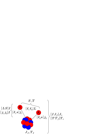
Figure 1: Angular momentum and isospin coupling schemes used in the calculations. The projectile initial (ground) state and final residue state have spin $J_{i}$ (projection $M_{i})$ and $J_{f}$ (projection $M_{f})$ and isospins $T_{i}$ (projection $\tau_{i})$ and $T_{f}$ (projection $\tau_{f})$, respectively. Each two nucleon configuration $\alpha$ involves of a pair of active orbitals $\beta_{1}$ and $\beta_{2}$ with spherical shell-model quantum numbers $n_{i}$, $\ell_{i}$ and $j_{i}$ (projections $\lambda_{i}$ and $m_{i})$. In $LS$-coupling, the nucleon orbital angular momenta $\ell_{1}$ and $\ell_{2}$ are coupled to $L$ (projection $\Lambda)$, the intrinsic spins to $S$ (projection $\Sigma)$ and $L$ and $S$ to a total angular momentum $I$, which must also couple the initial and final state total angular momenta.

It is convenient to combine the statistical factors and $9j$ coefficient from the two-nucleon overlap with the appropriate $jj$-coupled TNA to construct a set of $LS$-coupled TNA, $\mathfrak{C}$, as

$$\mathfrak{C}_{\alpha{LS}}^{IT}= \,\hat{j}_{1}\,\hat{j}_{2}\,\hat{L}\,\hat{S}\,\left\{\begin{array}[]{ccc}\ell_{1}&s&j_{1}\\ \ell_{2}&s&j_{2}\\ L&S&I\\ \end{array}\right\}\,C_{\alpha}^{IT}\ ,$$ (10)

that satisfy the sum rule

$$\sum_{LS}\left[\mathfrak{C}_{\alpha{LS}}^{IT}\right]^{2}=\left[C_{\alpha}^{IT}\right]^{2}\ .$$ (11)

Antisymmetry requires, for configurations $\alpha$ where the nucleons originate from the same orbital, the $[n\ell j]^{2}$ cases, that $L+S+T$ is odd. For nucleons originating from different orbitals this is no longer the case; though for two nucleons from spin-orbit partner orbitals, $[n\ell{j_{<}},n\ell{j_{>}}]$ with very similar radial wave functions, the $L+S+T=$even amplitudes are also expected to be significantly suppressed.

II.2 Eikonal model of two-nucleon stripping

As was developed previously TPB04 ; ToB06 ; STB09b , we exploit eikonal reaction dynamics. The elastic $S$-matrices describing the absorptive interactions of the $A$-body core (in state $f$) and the two nucleons with the target are calculated in the optical limit of Glauber’s multiple scattering theory Gla59 ; ATT96 assuming that these projectile constituents travel on straight line paths in the interaction field of the light target. The reaction is assumed sudden, such that the projectile internal co-ordinates are frozen on the timescale of this passing and interaction with the target. The eikonal $S$-matrices are calculated from the nucleon- and heavy residue-target interactions. These interactions were obtained by double-folding the residue (core), nucleon ($\delta$-function) and the target point particle densities with the usual effective nucleon-nucleon interaction, as used elsewhere; e.g. TPB04 .

Following Refs. TPB04 ; ToB06 ; STB09b , from the total absorption cross section for the projectile-target system,

$$\sigma_{abs}=\frac{1}{\hat{J}_{i}^{2}}\sum_{M_{i}}\int{d{\boldsymbol{b}}}\bra{\Psi_{i}}1-|\mathcal{S}_{f}\mathcal{S}_{1}\mathcal{S}_{2}|^{2}\ket{\Psi_{i}}\ ,$$ (12)

that includes all events where one or more of the projectile constituents are absorbed by the target, we can identify and extract the two-nucleon stripping cross section terms,

$$\sigma_{str}=\frac{1}{\hat{J}_{i}^{2}}\sum_{M_{i}}\int{d{\boldsymbol{b}}}\bra{\Psi_{i}}|\mathcal{S}_{f}|^{2}(1-|\mathcal{S}_{1}|^{2})(1-|\mathcal{S}_{2}|^{2})\ket{\Psi_{i}}\ .$$ (13)

As has been discussed elsewhere STB09b , the two-nucleon stripping probability $\mathcal{O}_{str}(b,b_{1},b_{2})=|\mathcal{S}_{f}|^{2}(1-|\mathcal{S}_{1}|^{2})(1-|\mathcal{S}_{2}|^{2})$ weights the impact parameters that contribute to these stripping events. Stripping requires an absorptive (inelastic) interaction of two nucleons with the target, but a non-absorptive (elastic) or non-interaction of the heavy residue with the target, and strongly localizes the reaction to grazing collisions at the projectile surface. This simplifies our picture of the reaction mechanism and of that part of the overlap function that is probed in the knockout reaction. We also contrast the present strong surface localisation of the reaction with the term peripheral used by some authors to mean impact parameters that sample only the extreme tail (the Whittaker or Hankel function asymptotics) of the nucleon bound state wave function. This is certainly not the case for those impact parameters selected by $\mathcal{O}_{str}(b,b_{1},b_{2})$ at the projectile energies and with the corresponding absorptive $S$-matrices of interest here.

Two further assumptions are made. The most important, but which is supported by the stripping mechanism’s selection of non-absorptive or non-interactive events of the residue and target, is to assume there is no dynamical excitation/change of state of the reaction residue by $\mathcal{S}_{f}$ in the collision – previously termed the spectator core approximation. This being the case,

$$\bra{\Phi^{(F^{\prime})}(A)} |\mathcal{S}_{f}|^{2}\ket{\Phi^{(F)}(A)}=|\mathcal{S}_{c}|^{2}\delta_{FF^{\prime}}\ ,$$ (14)

where the bra and ket integrate out the internal coordinates of the residue and $\mathcal{S}_{c}$ is taken to be the residue ground state-target elastic scattering $S$-matrix. A lesser assumption is the heavy-core (no-recoil) approximation, that in the required integrals, such as Eq. (13), the residue impact parameter $b_{c}$, entering $\mathcal{S}_{f}$ can be replaced by that of the center of mass of the projectile $b$, i.e. $b_{c}\approx b$. For the stripping terms this approximation is not in fact needed, as a change of integration variable makes it unnecessary.

The result of these assumptions, together with the parentage expansion for the two nucleon structure overlap, Eq. (1), is that the exclusive stripping cross section to a given final state $f$ can be written

$$\sigma_{str}^{(f)}=\int{d{\boldsymbol{b}}}\,|\mathcal{S}_{c}|^{2}\frac{1}{\hat{J}_{i}^{2}}\sum_{M_{i}M_{f}} \bra{\Psi_{i}^{(F)}}(1-|\mathcal{S}_{1}|^{2})$$

$$(1-|\mathcal{S}_{2}|^{2})\ket{\Psi_{i}^{(F)}}\ .$$ (15)

The assumption that the nucleon $S$-matrices are spin-independent allows one to carry out all spin coordinate sums, in preparation for which we separate explicitly the nucleon position and spin variable integrations, as

$$\bra{\Psi_{i}^{(F)}} \ldots\ket{\Psi_{i}^{(F)}}$$

$$= \int{d{\boldsymbol{r}}_{1}}\int{d{\boldsymbol{r}}_{2}}\braket{\Psi_{i}^{(F)}}{\ldots}{\Psi_{i}^{(F)}}_{sp}\ ,$$ (16)

where the final bra-ket term denotes the spin integration.

Consideration of this (momentum-integrated) stripping cross section using $LS$-coupling was made in Ref. TPB04 , there with an emphasis on the reaction mechanism’s lack of selectivity in the total spin $S$ of the two nucleons. In our previous analysis of the longitudinal momentum distributions STB09b the only angular momentum projections not able to be summed over algebraically were those of the orbital angular momenta of the two nucleons.

This observation made, we now consider the residue longitudinal momentum distributions in the $LS$-representation. The derivation follows a similar pattern to that in the $jj$-coupled algebra and begins from the $LS$-coupled, spin-integrated, modulus squared of the two-nucleon overlap, averaged over initial projections $M_{i}$ and summed over final projections $M_{f}$. Explicitly,

$$\frac{1}{\hat{J}_{i}^{2}}\sum_{M_{i}M_{f}} \braket{\Psi_{i}^{(F)}}{\Psi_{i}^{(F)}}_{sp}=\frac{1}{\hat{J}_{i}^{2}}\sum_{\begin{subarray}{c}II^{\prime}\mu\mu^{\prime}\\ \alpha\alpha^{\prime}TT^{\prime}\end{subarray}}C_{\alpha}^{IT}C_{\alpha^{\prime}}^{I^{\prime}T^{\prime}}$$

$$\times \sum_{M_{i}M_{f}}(I\mu J_{f}M_{f}|J_{i}M_{i})\,(I^{\prime}\mu^{\prime}J_{f}M_{f}|J_{i}M_{i})$$

$$\times \ (T{\tau}T_{f}\tau_{f}|T_{i}\tau_{i})\,(T^{\prime}{\tau}^{\prime}T_{f}\tau_{f}|T_{i}\tau_{i})$$

$$\times \Braket{[\,\overline{\psi_{j_{1}^{\prime}}(1)\otimes\psi_{j_{2}^{\prime}}(2)}\,]_{I^{\prime}\mu^{\prime}}^{T^{\prime}\tau^{\prime}}}{[\,\overline{\psi_{j_{1}}(1)\otimes\psi_{j_{2}}(2)}\,]_{I\mu}^{T\tau}}_{sp}.$$ (17)

On performing the sums over $M_{i}$ and $M_{f}$ the expression is clearly incoherent in the coupled two-nucleon total angular momentum $I\mu$, a consequence of the spectator-core approximation, Eq. (14). Using the antisymmetric two-nucleon $LS$-coupled forms of Eqs. (5) and (10), and assuming the nucleon $S$-matrices are also isospin-independent, we can perform the isospin sums with the result that Eq. (17) is also incoherent with respect to both $S$ and $T$. Finally, summing over the projections of $I$ and $S$ we obtain the result, incoherent also in $L$ and $\Lambda$, namely

$$\frac{1}{\hat{J}_{i}^{2}} \sum_{M_{i}M_{f}}\braket{\Psi_{i}^{(F)}}{\Psi_{i}^{(F)}}_{sp}$$

$$= \sum_{T}(T{\tau}T_{f}\tau_{f}|T_{i}\tau_{i})^{2}\sum_{ILS\alpha\alpha^{\prime}}\frac{\mathfrak{C}_{\alpha{LS}}^{IT}\mathfrak{C}_{\alpha^{\prime}{LS}}^{IT}D_{\alpha}D_{\alpha^{\prime}}}{\hat{L}^{2}}$$

$$\sum_{\Lambda\lambda_{1}\lambda_{2}\lambda_{1}^{\prime}\lambda_{2}^{\prime}}(\ell_{1}\lambda_{1}\ell_{2}\lambda_{2}|L\Lambda)(\ell_{1}^{\prime}\lambda_{1}^{\prime}\ell_{2}^{\prime}\lambda_{2}^{\prime}|L\Lambda)$$

$$[\psi_{\beta_{1}^{\prime}}^{\lambda_{1}^{\prime}}({\boldsymbol{r}}_{1})\psi_{\beta_{2}^{\prime}}^{\lambda_{2}^{\prime}}({\boldsymbol{r}}_{2})-(-)^{S+T}\psi_{\beta_{1}^{\prime}}^{\lambda_{1}^{\prime}}({\boldsymbol{r}}_{2})\psi_{\beta_{2}^{\prime}}^{\lambda_{2}^{\prime}}({\boldsymbol{r}}_{1})]^{*}$$

$$[\psi_{\beta_{1}}^{\lambda_{1}}({\boldsymbol{r}}_{1})\psi_{\beta_{2}}^{\lambda_{2}}({\boldsymbol{r}}_{2})-(-)^{S+T}\psi_{\beta_{1}}^{\lambda_{1}}({\boldsymbol{r}}_{2})\psi_{\beta_{2}}^{\lambda_{2}}({\boldsymbol{r}}_{1})]\ .$$ (18)

The exclusive two-nucleon stripping cross section is then given by use of this structure overlap information in Eq. (15). In the following we derive explicit expressions for the associated exclusive momentum distributions in this $LS$-representation.

II.3 Residue momentum distributions

Structurally, the expressions for the residue momentum distributions in the $LS$-coupling scheme are similar to those using $jj$-coupling STB09b . The derivations also follow a largely parallel procedure. The coordinate system used is reproduced in Fig. 2 for clarity of the following expressions.

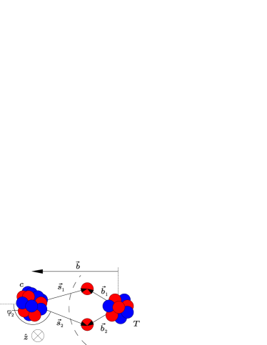
Figure 2: Schematic of the particle coordinates used. Vectors ${\boldsymbol{s}}_{i}$ are the components, in the plane perpendicular to the beam direction (the $z$-axis), of the position vectors ${\boldsymbol{r}}_{i}$ of the knocked-out nucleons relative to the core of nucleons to which they are initially bound. The two nucleons have impact parameters ${\boldsymbol{b_{i}}}={\boldsymbol{b}}+{\boldsymbol{s}}_{i}$ relative to the target nucleus.

The reaction samples the momentum content of the bound-state wave functions of the stripped nucleons in the direction of the projectile beam $\hat{{\boldsymbol{k}}}$ (i.e. the $z$-axis). For fixed values of the ${\boldsymbol{s}}_{i}$, and hence fixed nucleon impact parameters ${b}_{i}=|{\boldsymbol{b}}+{\boldsymbol{s}}_{i}|,\ i=1,2$, this information is carried by the functions

$$\mathcal{R}_{\beta}^{\lambda}\!(i)\, =\frac{\mathcal{C}_{\ell\lambda}}{\sqrt{2\pi}}\int^{+\infty}_{-\infty}\;dz_{i}\;u_{\beta}(r_{i})\;P_{\ell}^{|\lambda|}(\cos\theta_{i})\exp[i{\kappa_{i}}z_{i}]\ ,$$ (19)

where $\kappa_{i}$ is the $z$-component of the momentum of nucleon $i$ in the projectile’s rest-frame. We note that the notation for $\mathcal{R}_{\beta}^{\lambda}\!(i)\,$ is changed from that of Ref. STB09b consistent with the notation used for the $u_{\beta}(r_{i})$. The correct weighting of the nucleon absorption probability with the azimuthal angle $\varphi_{i}$, of ${\boldsymbol{s}}_{i}$, is carried by the functions $\mathcal{H}_{\lambda\lambda^{\prime}}(i)\equiv\mathcal{H}_{\lambda\lambda^{\prime}}(b,{\boldsymbol{s}}_{i})$, given by

$$\mathcal{H}_{\lambda\lambda^{\prime}}(i) =\int_{0}^{2\pi}d{\varphi_{i}}(1-|\mathcal{S}_{i}(|{\boldsymbol{b}}+{\boldsymbol{s}}_{i}|)|^{2})\exp[i\varphi_{i}(\lambda-\lambda^{\prime})]\ ,$$ (20)

with ${\boldsymbol{s}}_{i}$ the components of the ${\boldsymbol{r}}_{i}$ in the impact parameter plane, i.e. ${\boldsymbol{r}}_{i}={\boldsymbol{s}}_{i}+z_{i}\hat{{\boldsymbol{k}}}$. The remaining details of the derivation are completely analogous to those in Ref. STB09b , to which the reader is referred.

We obtain the projectile rest frame, stripping mechanism momentum distribution as the incoherent $LS$ and isospin decomposition

$$\frac{d\sigma_{str}^{(f)}}{d\kappa_{c}}= \sum_{LST}\frac{d\sigma_{LST}^{(f)}}{d\kappa_{c}}$$

$$= \sum_{T}(T{\tau}T_{f}\tau_{f}|T_{i}\tau_{i})^{2}\sum_{LSI\alpha\alpha^{\prime}}\frac{2\mathfrak{C}_{\alpha{LS}}^{IT}\mathfrak{C}_{\alpha^{\prime}{LS}}^{IT}D_{\alpha}D_{\alpha^{\prime}}}{\hat{L}^{2}}$$

$$\int{d\kappa_{1}}\int{d\kappa_{2}}\;\delta(\kappa_{c}+\kappa_{1}+\kappa_{2})\int{d{\boldsymbol{b}}}\;|\mathcal{S}_{c}(b)|^{2}$$

$$\sum_{\Lambda\lambda_{1}\lambda_{2}\lambda_{1}^{\prime}\lambda_{2}^{\prime}}(\ell_{1}\lambda_{1}\ell_{2}\lambda_{2}|L\Lambda)(\ell_{1}^{\prime}\lambda_{1}^{\prime}\ell_{2}^{\prime}\lambda_{2}^{\prime}|L\Lambda)$$

$$\int{ds_{1}}s_{1}\int{ds_{2}}s_{2}\left[direct-exchange\right],$$ (21)

where the direct term is

$$direct= \left\{\mathcal{H}_{\lambda_{1}\lambda_{1}^{\prime}}(1)\mathcal{R}_{\beta_{1}}^{\lambda_{1}}\!(1)\,\mathcal{R}_{\beta_{1}^{\prime}}^{\lambda_{1}^{\prime}}\!(1)^{*}\,\right.$$

$$\times \left.\mathcal{H}_{\lambda_{2}\lambda_{2}^{\prime}}(2)\mathcal{R}_{\beta_{2}}^{\lambda_{2}}\!(2)\,\mathcal{R}_{\beta_{2}^{\prime}}^{\lambda_{2}^{\prime}}\!(2)^{*}\,\right\},$$ (22)

and the exchange term,

$$exchange= (-1)^{S+T}\left\{\rule{0.0pt}{12.0pt}\mathcal{H}_{\lambda_{2}\lambda_{1}^{\prime}}(1)\mathcal{R}_{\beta_{2}}^{\lambda_{2}}\!(1)\,\mathcal{R}_{\beta_{1}^{\prime}}^{\lambda_{1}^{\prime}}\!(1)^{*}\,\right.$$

$$\times \left.\mathcal{H}_{\lambda_{1}\lambda_{2}^{\prime}}(2)\mathcal{R}_{\beta_{1}}^{\lambda_{1}}\!(2)\,\mathcal{R}_{\beta_{2}^{\prime}}^{\lambda_{2}^{\prime}}\!(2)^{*}\,\right\}\ .$$ (23)

It should be noted that Eq. (21) (that contains a factor of 2) and these simplified forms for the direct and exchange terms compared to STB09b , assume that both the integrals over the $\kappa_{i}$ and the $s_{i}$ will be carried out, and so one is computing quantities that are completely symmetric in the two nucleon coordinates. Also, unlike for the $jj$-coupled scheme, no further re-coupling is required to reduce the angular momentum algebra.

Physically, Eq. (21) shows that the sums of the direct and exchange terms over the $\lambda$ are independent of $I$. The resulting momentum distributions thus depend explicitly on $L$ (and $S+T$ via the phase of the exchange term), but not on $I$. We see that the significance of $I$ and the nucleon total angular momenta $j_{i}$ is that they will determine the relative strengths of the different $L$ and $S$ via the amplitudes $\mathfrak{C}_{\alpha{LS}}^{IT}$. Thus it is $L$, and to a lesser extent $S$ and $T$, that will determine the shape of the residue’s momentum distribution. $I$ on the other hand will be important in determining the relative strengths of the $L$ and $S$ that contribute.

III Two-nucleon correlations

We observe that the expression for residue momentum distributions is somewhat simpler when using $LS$-coupling, having a more transparent angular momentum dependence. However, the dependence on the two nucleon configurations, via $\alpha$ (and $\alpha^{\prime}$), is still less than transparent in Eq. (21). We attempt to elucidate this important nuclear structure sensitivity by carrying out the $\lambda$ projections sums. Before doing so we introduce and discuss the two-nucleon joint position probability that summarizes both the strength and the spatial localisation (and correlation) of the two nucleons in the structure overlaps that affects the stripping yield.

III.1 Two-nucleon joint position probability

We consider the two-nucleon joint position probability relevant to the removal reaction/transition to a given final state $f$, i.e.

$$\rho_{f}({\boldsymbol{r}}_{1},{\boldsymbol{r}}_{2}) =\frac{1}{\hat{J}_{i}^{2}}\sum_{M_{i}M_{f}}\braket{\Psi_{i}^{(F)}}{\Psi_{i}^{(F)}}_{sp}\ .$$ (24)

While the production of a given residue final state by the two-nucleon knockout mechanism will depend on the details of $\rho_{f}({\boldsymbol{r}}_{1},{\boldsymbol{r}}_{2}$), specifically the extent to which there is a spatial proximity of the two nucleons at the projectile surface, its overall normalisation and the $LS$-composition of this normalisation

$$N_{f}= \int\!{d{\boldsymbol{r}}_{1}}\int\!{d{\boldsymbol{r}}_{2}}\;\rho_{f}({\boldsymbol{r}}_{1},{\boldsymbol{r}}_{2})$$

$$= \sum_{\alpha IT}\left[(T{\tau}T_{f}\tau_{f}|T_{i}\tau_{i})C_{\alpha}^{IT}\right]^{2}$$

$$= \sum_{LS}\left\{\sum_{\alpha IT}\left[(T{\tau}T_{f}\tau_{f}|T_{i}\tau_{i})\mathfrak{C}_{\alpha{LS}}^{IT}\right]^{2}\right\}=\sum_{LS}N_{f}^{LS},$$ (25)

are measures of the likely transition strength. In the case of a single (dominant) two-nucleon structure configuration this $LS$ breakdown can also guide the relative strengths expected from the different contributing $LS$ terms for a given final state. However, when configurations are mixed or where the initial and final states have different parity, interference effects may strongly affect these relative strengths.

Since the projectile is assumed to traverse a straight line path in the $z$-direction, it is useful for what follows, and also highly intuitive, to construct the projection of the two-nucleon joint position probability onto the impact parameter plane – the plane perpendicular to the beam direction – by integration over the $z_{i}$ of the two nucleons,

$$\mathcal{P}_{f}({\boldsymbol{s}}_{1},{\boldsymbol{s}}_{2})=\int\!{dz_{1}}\int\!{dz_{2}}\;\rho_{f}({\boldsymbol{r}}_{1},{\boldsymbol{r}}_{2})\ .$$ (26)

The relevant spatial correlation for the reaction is now the degree of localisation of the probability with respect to the two nucleon coordinate projections ${\boldsymbol{s}}_{i}$ in this impact parameter plane.

In what follows the correlation of the two nucleons is concisely expressed as a function of the angular separation, $\omega$, of their position coordinates ${\boldsymbol{r}}_{i}$. Clearly, the $z_{i}$ integrated joint probability $\mathcal{P}_{f}({\boldsymbol{s}}_{1},{\boldsymbol{s}}_{2})$ will see a smeared version of this correlation function since fixed ${\boldsymbol{s}}_{i}$ will sample a range of $\omega$. However, since the reaction is surface localized and the target is light (small) the effective thickness in the $z_{i}$ will tend to be rather restricted and $\mathcal{P}_{f}({\boldsymbol{s}}_{1},{\boldsymbol{s}}_{2})$ will remain a useful construct and intuitive link to the magnitudes of the two-nucleon knockout cross sections.

As was indicated by Figs. 2 and 3 of Ref. senuf06 , and will be emphasized here, the total angular momentum of the final state and the detailed TNA of the wave function can strongly affect the two-nucleon joint position probability, its projection and the magnitude of the removal cross sections. The (shell-model) structural correlations may also enhance or suppress particular total orbital angular momenta and so may affect the residue momentum distributions also.

III.2 Angular Correlations

Despite the relative simplifications introduced by $LS$-coupling, the momentum distribution expression, Eq. (21), remains a complicated weighted sum of wave function transforms. Moreover, it still depends on the orbital angular momentum projections. To clarify the underlying sensitivity to two-nucleon correlations we simplify the spin-integrated two-nucleon joint position probability of Eq. (24) by summing out the $\lambda$ projection labels.

The relevant terms we need to simplify are, for the direct terms of Eq. (18),

$$\Gamma_{\ell_{1}\ell_{2}\ell_{1}^{\prime}\ell_{2}^{\prime}}^{L}(\hat{{\boldsymbol{r}}}_{1},\hat{{\boldsymbol{r}}}_{2})= \sum_{\Lambda\lambda_{1}\lambda_{2}\lambda_{1}^{\prime}\lambda_{2}^{\prime}}(\ell_{1}\lambda_{1}\ell_{2}\lambda_{2}|L\Lambda)(\ell_{1}^{\prime}\lambda_{1}^{\prime}\ell_{2}^{\prime}\lambda_{2}^{\prime}|L\Lambda)$$

$$\times Y_{\ell_{1}\lambda_{1}}(\hat{{\boldsymbol{r}}}_{1})Y^{*}_{\ell_{1}^{\prime}\lambda_{1}^{\prime}}(\hat{{\boldsymbol{r}}}_{1})Y_{\ell_{2}\lambda_{2}}(\hat{{\boldsymbol{r}}}_{2})Y^{*}_{\ell_{2}^{\prime}\lambda_{2}^{\prime}}(\hat{{\boldsymbol{r}}}_{2}).$$ (27)

Combining the spherical harmonics of the same argument, summing the $\lambda$ projections, and using the spherical harmonics addition theorem one obtains

$$\Gamma_{\ell_{1}\ell_{2}\ell_{1}^{\prime}\ell_{2}^{\prime}}^{L}(\omega)= (-1)^{L}\frac{\hat{\ell}_{1}\hat{\ell}_{1}^{\prime}\hat{\ell}_{2}\hat{\ell}_{2}^{\prime}\hat{L}^{2}}{(4\pi)^{2}}\sum_{k}W(\ell_{1}\ell_{2}\ell_{1}^{\prime}\ell_{2}^{\prime};Lk)$$

$$\times (-1)^{k}(\ell_{1}0\ell_{1}^{\prime}0|k0)(\ell_{2}0\ell_{2}^{\prime}0|k0)P_{k}(\cos\omega),$$ (28)

where $\omega$ is the angular separation of the two nucleons, i.e. $\cos\omega={\boldsymbol{r}}_{1}\cdot{\boldsymbol{r}}_{2}/r_{1}r_{2}$. A similar result can be found in Ref. BBR67 .

The angular correlation function $\Gamma_{\ell_{1}\ell_{2}\ell_{1}^{\prime}\ell_{2}^{\prime}}^{L}(\omega)$ is seen to be independent of the total angular momentum $I$ and of the individual angular momenta $j_{i}$ of the nucleons. However, it depends explicitly on their orbital angular momenta and on the total orbital angular momentum $L$. The form written above is that for the direct terms of Eq. (18). The exchange terms differ by a phase due to the reordering of the angular momentum labels in the exchange form of Eq. (27), as is given below.

The radial behaviors associated with the direct and exchange terms of the joint-probability density are

$$U_{\alpha\alpha^{\prime}}^{D}(r_{1},r_{2})= \;u_{\beta_{1}}(r_{1})\;u_{\beta_{2}}(r_{2})\;u_{\beta_{1}^{\prime}}(r_{1})\;u_{\beta_{2}^{\prime}}(r_{2})$$

$$+ \,u_{\beta_{2}}(r_{1})\;u_{\beta_{1}}(r_{2})\;u_{\beta_{2}^{\prime}}(r_{1})\;u_{\beta_{1}^{\prime}}(r_{2})\ ,$$

$$U_{\alpha\alpha^{\prime}}^{E}(r_{1},r_{2})= \;u_{\beta_{1}}(r_{1})\;u_{\beta_{2}}(r_{2})\;u_{\beta_{2}^{\prime}}(r_{1})\;u_{\beta_{1}^{\prime}}(r_{2})$$

$$+ \,u_{\beta_{2}}(r_{1})\;u_{\beta_{1}}(r_{2})\;u_{\beta_{1}^{\prime}}(r_{1})\;u_{\beta_{2}^{\prime}}(r_{2})\ .$$ (29)

In terms of these and the corresponding direct and exchange angular correlation functions, the two-nucleon joint-probability density is

$$\rho_{f}({\boldsymbol{r}}_{1},{\boldsymbol{r}}_{2})= \sum_{LST}\sum_{I\alpha\alpha^{\prime}}\frac{\mathfrak{C}_{\alpha{LS}}^{IT}\mathfrak{C}_{\alpha^{\prime}{LS}}^{IT}D_{\alpha}D_{\alpha^{\prime}}}{\hat{L}^{2}}(T{\tau}T_{f}\tau_{f}|T_{i}\tau_{i})^{2}$$

$$\times \left[U_{\alpha\alpha^{\prime}}^{D}(r_{1},r_{2})\,\Gamma^{L,D}(\omega)\right.$$

$$- \left.(-)^{S+T}U_{\alpha\alpha^{\prime}}^{E}(r_{1},r_{2})\,\Gamma^{L,E}(\omega)\right],$$ (30)

with $\Gamma^{L,D}(\omega)\equiv\Gamma_{\ell_{1}\ell_{2}\ell_{1}^{\prime}\ell_{2}^{\prime}}^{L}(\omega)$ given by Eq. (28) and

$$\Gamma^{L,E}(\omega)=(-)^{\ell_{1}^{\prime}+\ell_{2}^{\prime}-L}\,\Gamma_{\ell_{1}\ell_{2}\ell_{2}^{\prime}\ell_{1}^{\prime}}^{L}(\omega)\,.$$ (31)

It is clear therefore that the angular correlation function dictates how the spatial correlations change with angular momentum coupling, and that $L$ is crucial, the $U(r_{1},r_{2})$ being dependent on the $\beta_{i}$ but independent of the angular momentum coupling. Clear also is that, in cases where the radial wave functions for all active orbits are similar, the angular correlation function alone will determine the differences in residue momentum distributions for the different possible angular momentum couplings. As was discussed earlier, these differences, generated at the angular correlation function and the two-nucleon density level, will be more distinct than in the projected density, Eq. (26) where fixed co-ordinate pairs $({\boldsymbol{s}}_{1},{\boldsymbol{s}}_{2})$ sample a range of angular separations $\omega$ and so will smear the spatial correlations.

Uncorrelated two nucleon models, discussed in the Introduction and Refs. BBC03 ; TPB04 , that neglect antisymmetrization, angular momentum coupling and parentage coefficients lead to a constant, $\omega$-independent correlation function. For two nucleon removal from a single $[s_{1/2}]^{2}$ configuration, the angular correlation function is also seen to be $\omega$-independent ($k=0$) and the uncorrelated (see Ref. STB09b ) and fully correlated residue momentum distributions will be identical.

III.3 Cross shell excitations

Here we consider briefly the implications for two-nucleon knockout from configurations with $\beta_{1}$ and $\beta_{2}$ of different parity. It is well established that the addition of shell-model configurations with $1\hbar\omega$, $3\hbar\omega$ single particle excitations are required to obtain a high degree of surface pairing (see e.g. Pin84 ; JaL83 ; CIM84a ; CIM84b ; IJM89 ; TTD98 ).

We obtain a similar result here, by considering the symmetry of the angular correlation function about $\omega=\pi/2$. In $\Gamma_{\ell_{1}\ell_{2}\ell_{1}^{\prime}\ell_{2}^{\prime}}^{L}(\omega)$, only the Legendre polynomial depends on $\omega$, with the property that $P_{k}(\cos[\pi-\omega])=(-1)^{k}P_{k}(\cos\omega)$. Since the values of $k$ are restricted to be odd or even by the parity Clebsch Gordan coefficients, the angular correlation will be even about $\pi/2$ for $\pi_{\ell}\pi_{\ell^{\prime}}=+1$ and odd about $\pi/2$ for $\pi_{\ell}\pi_{\ell^{\prime}}=-1$. In the absence of single-particle excitations of the kind $1\hbar\omega$, the probability for finding the nucleon pair with angular separation $\omega=0$ and $\pi$ are equal and a high degree of two-nucleon pair/cluster structure will not be obtained.

So, pair correlations will be enhanced in cases when there is mixing between two-nucleon configurations where the orbital angular momenta are of different parity. Whether the interference is constructive or destructive will depend on the sign of $\Gamma_{\ell_{1}\ell_{2}\ell_{1}^{\prime}\ell_{2}^{\prime}}^{L}(\omega)$ near $\omega=0$, the relative signs of the $9j$ coefficients, and the relative signs of the TNA. A specific two configuration example will be presented in the Section IV.3 below.

These results are quite general in that they do not depend on the pair total angular momentum $I$; enhancements in the spatial correlations in the two-nucleon density may be found for $I\neq 0$.

IV Illustrative examples

Previous calculations of exclusive two-nucleon removal residue momentum distributions noted a strong sensitivity to the total angular momentum of the removed nucleon pair. Here, by writing this momentum-differential cross section in $LS$-coupling, and by a consideration of the angular correlations inherent in the two-nucleon joint probability function, it becomes apparent that the crucial sensitivity of this observable is to the total orbital angular momentum values, $L$, contributing to the transition. These different $L$ components will contribute incoherently to the cross section yields and their momentum distributions. These theoretical observations and the resulting sensitivity of the momentum distribution observable offers the potential to probe more subtle features of the nucleon pair’s configurations and the correlations present in the shell-model wave functions used.

A generic first example will arise if the predominant two-nucleon configuration populating a given final state involves one of the nucleons in an $s$-wave orbital. In this case the total orbital angular momentum is restricted to the orbital angular momentum of the second active orbit, $L=\ell$, and thus $L$ is pure. It is expected therefore that there can be distinct differences in the momentum distributions, even for states of the same total angular momentum $I$. For example, for two $3^{+}$ final states built from $[g_{7/2},s_{1/2}]$ and from $[d_{5/2},s_{1/2}]$. More generally, even where there is significant mixing and several active configurations, the structure of specific states in the spectrum can be rather $L$-pure. So, the reaction will proceed by a particular $L$ with a momentum distribution that is characteristic of this structure.

In the following we discuss specific examples from different $A$ and $Z$ regions of the nuclear chart. In each example the nucleon bound state radial wave functions required for the two-nucleon overlaps are calculated using a Woods-Saxon potential well with a spin-orbit term of depth 6 MeV and a diffuseness parameter $a_{0}$=0.7 fm. Unless stated otherwise, the geometries (the radius parameters $r_{0}$) of the potential wells in each case were adjusted to reproduce the root mean square radii and the separation energies of spherical Hartree-Fock calculations using the Skyrme (SkX) interaction parameterization brown98 for the active orbitals in question. The specific procedure was detailed in Ref. Gad08 . These fitted geometries are then used to calculate the radial wave functions needed using the empirical, effective nucleon separation energies. Where required, shell-model calculations are performed using the code oxbash BEG04 . The model spaces and interactions used are specified for each case studied, below.

IV.1 p-shell example: ¹²C(-np)

Here we consider the removal of a ($T=0,1$) neutron and proton ($np$) pair from ¹²C at 2100 MeV/nucleon on a ¹²C target. The proton and neutron orbits are taken to be identical with radial wave functions calculated in a Woods-Saxon potential, using an average nucleon charge $\bar{Z}=0.5$. The geometry of the Woods-Saxon potential was fixed with $r_{0}=1.31$ fm, $a_{0}=0.7$ fm. Both the ¹⁰B residue and ¹²C target were assumed have Gaussian shaped mass distributions, with rms radii 2.30 and 2.32 fm respectively. The isospin format TNA are calculated using oxbash in a $p$-shell model space using the wbp interaction WaB92 , as in previous studies BHS02 ; TBP04 . A more complete consideration of two-nucleon removal from ¹²C will be discussed in a forthcoming paper ToS10 .

As a specific example, we consider the first and second $T=0$, ¹⁰B($1^{+}$) final states. The TNA for these states are shown in Table 1. The relative magnitudes of the contributing two-nucleon configurations to these states are different and it is of interest to consider how these differences might affect the cross sections and their momentum distributions. The sum of the squared TNA for the first and second states are 1.45 and 1.47, respectively, thus in the absence of interference terms the incoherent sum of contributions from each of these configurations would yield very similar cross sections.

That this is not the case is shown by the calculated two-nucleon stripping cross sections presented in Table 2. The calculated momentum distributions are also rather different, as is shown in Fig. 3.

Table 1: Isospin format two nucleon amplitudes for the first and second ¹⁰B($1^{+}$) $T=0$ states populated by neutron-proton removal from ¹²C. The relative strengths of the two nucleon amplitudes are different for the two states.

$J_{f}^{\pi}$	$[1p_{3/2}]^{2}$	$[1p_{1/2},1p_{3/2}]$	$[1p_{1/2}]^{2}$
1${}_{1}^{+}$	0.69899	0.97868	$-$0.01067
1${}_{2}^{+}$	$-$1.13385	0.22886	0.36314

Table 2: Two-neutron stripping cross sections $\sigma_{LS}$ for populating the first two $T=0,J_{f}=1^{+}$ final states in ¹⁰B for a ¹²C beam energy of 2100 MeV per nucleon. All cross sections are in mb.

$J_{f}^{\pi}$	$\sigma_{01}$	$\sigma_{10}$	$\sigma_{11}$	$\sigma_{21}$	$\sigma_{str}$
1${}_{1}^{+}$	2.41	0.00	0.00	0.06	2.47
1${}_{2}^{+}$	0.60	0.59	0.00	0.63	1.81

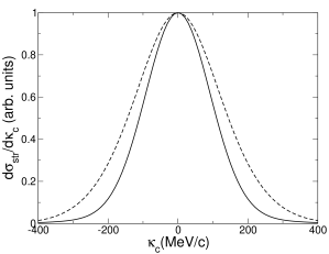
Figure 3: Normalized residue momentum distributions for the first (solid) and second (dashed) ¹⁰B($J_{f}$=1⁺) states populated in $np$ knockout from ¹²C at 2100 MeV per nucleon. Though the same two-nucleon configurations contribute to each state, the differently weighted TNA result in distinct momentum distributions.

These differences can be understood by reference to the projected two-particle joint position probabilities for the two states, which are strikingly different. The first $1^{+}$ state shows strong spatial localisation of the two-nucleons, favorable for the two-nucleon removal cross section. Both example position probabilities manifest the expected symmetry about a nucleon angular separation of $\phi_{12}=\pi/2$, since the model space is restricted to the $p$-shell and the active orbitals have the same parity.

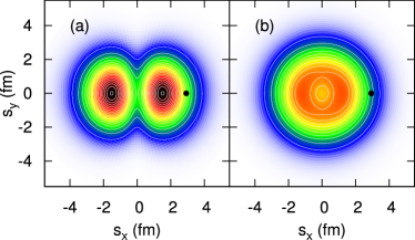
Figure 4: (Color online) Impact parameter plane-projected joint position probabilities for (a) the first and (b) second $T=0$ ¹⁰B(1⁺) states populated via $np$ knockout from ¹²C. The plot shows the impact parameter plane probability distribution of nucleon 2 for nucleon 1 positioned at $s_{x}=2.9$ fm, $s_{y}=0$ fm. The spatial correlations of the nucleon pairs in these two states are fundamentally different, leading to markedly different momentum distributions; see Fig. 3. The color scale (white-blue-green-yellow-red-black) is common to both plots.

We can extend this $p$-shell example further to illustrate the potential for large sensitivity to the underlying structure. It is clear from Eq. (30) that within a $p$-shell model space the relative strengths of different $LS$ combinations are determined solely by the TNA and the nucleon configurations involved. So, neglecting any minor differences in the $p$-wave radial wave functions, due to spin-orbit splitting, the entire square bracketed term in Eq. (30) is independent of the total angular momenta $\{j_{i}\}$ and, in the present model space, independent of the configurations $(\alpha,\alpha^{\prime})$ of the pair. It follows that the weight of each $L$ and $S$ term in a state of given $I$ and $T$ is proportional to

$$P^{IT}_{LS}=\sum_{\alpha\alpha^{\prime}}\mathfrak{C}_{\alpha{LS}}^{IT}\mathfrak{C}_{\alpha^{\prime}{LS}}^{IT}D_{\alpha}D_{\alpha^{\prime}}\,.$$ (32)

In the sprit of studying the extremes of possible sensitivity of the momentum distributions, we may force any one of these $P^{IT}_{LS}$ to be zero, and solve for the relative strengths and phases of the $\mathfrak{C}_{\alpha{LS}}^{IT}$ and $C^{IT}_{\alpha}$ needed to achieve this.

Fig. 5 illustrates such examples for assumed $I=1$, $T=0$ states populated via the configurations $\alpha_{1}=[1p_{1/2}]^{2}$ and $\alpha_{2}=[1p_{3/2},1p_{1/2}]$. Calculations for two sets of TNA are shown; one set chosen to eliminate $L=0,S=1$ contributions (requiring $C_{\alpha_{1}}^{10}=-4C_{\alpha_{2}}^{10}$, dashed curve) and the other to eliminate $L=2,S=1$ contributions (requiring $C_{\alpha_{1}}^{10}=C_{\alpha_{2}}^{10}/2$, solid curve). These different $1^{+}$ state TNA produce wide and narrow residue momentum distributions, respectively, the difference in the FWHM widths being almost a factor of two. The figure also shows the $I=2,T=1$ momentum distribution (open circles), populated via $\alpha_{2}=[1p_{3/2},1p_{1/2}]$ and $\alpha_{3}=[1p_{3/2}]^{2}$, where the TNA were chosen to eliminate $L=2,S=1$ contributions (requiring $C_{\alpha_{3}}^{21}=-\sqrt{2}C_{\alpha_{2}}^{21}$). Once again this gives a relatively narrow distribution and, moreover, this $I=2$ distribution is narrower than that for the ($L=0$ excluded) $I=1$ distribution (dashed curve) described above. These examples break the tie between the width of the momentum distribution and the $I$ value of the transferred pair. Whether or not nuclear states with these TNA are physically realized, these limiting cases demonstrate how details of the microscopic structure of a given state may strongly influence the shapes and widths of the expected residue momentum distributions.

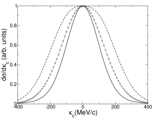
Figure 5: Theoretical ¹⁰B residue momentum distributions at 2100 MeV per nucleon. Shown are the expectations for two $I=1$ $T=0$ states where the TNA have been tailored to exclude $L=2,S=1$ (solid line) and $L=0,S=1$ (dashed line) contributions from the two-nucleon wave function, respectively. The line with open circles shows the expectation for an $I=2$ $T=1$ final state where the TNA were similarly chosen to eliminate $L=2,S=1$ contributions.

Similarly, we note the expectation that transitions to $I=2,T=0$ and $I=3,T=0$ states of ¹⁰B will, within a $p$-shell model space, yield identical theoretical momentum distributions since both transitions are pure $L=2$ in nature. In this instance also the width of the momentum distribution does not provide a direct measure of $J_{f}=I$.

We note that consideration has only been given to the direct population of ¹⁰B. In principle, indirect population by single nucleon knockout followed by evaporation of the unlike nucleon may be possible, although we expect this indirect, two-step pathway to be very weak, due to the large nucleon separation energies in the relevant $A=11$ systems and the very small predicted shell model strength for one nucleon removal to states above these first $A=11$ nucleon thresholds. High precision (stable beam) observations of final state exclusive ¹⁰B momentum distributions would clarify such aspects of the reaction mechanism that are currently assumed.

IV.2 sd-shell: ²⁸Mg(-2p) and ²⁶Si(-2n)

Exotic nuclei with valence nucleons in the $sd$-shell have been the focus of several two-nucleon removal experiments, studying the evolution of structure away from the valley of $\beta$-stability. The initial and final state structures are often well described within conventional $sd$-shell model space calculations offering good test cases for studies of the reaction mechanism. Details of their residue momentum distributions could offer an additional test of the shell model and the reaction mechanism in this region.

We first review the two-proton knockout from ²⁸Mg at 83.2 MeV/nucleon on a ⁹Be target, previously studied in Refs. BBC03 ; ToB06 ; STB09b . To date, this is the only experimental example with measured final-state exclusive ²⁶Ne momentum distributions. Four states were populated, being the $0^{+}$ ground state, the first and second $2^{+}$ states and the first $4^{+}$ state. Previous work demonstrated the significant difference between the ground state and $4^{+}$ residue momentum distributions, despite strong experimental (reaction target) broadening of the measured distributions.

We comment here on the effects on the 2.02 and 3.70 MeV $2^{+}$ state momentum distributions of the subtle differences in their TNA, tabulated in Ref. TPB04 . To remove the small difference in the average separation energies of the protons for the two states, calculations used identical radial wave functions, but this binding effect is in practice negligible. The calculated widths of the residue momentum distributions are different by $\sim 10\%$. Clearly a higher statistics experiment would be required to examine this difference predicted by the shell model. There are however other examples where the $sd$-shell model predicts TNA that exhibit a larger degree of sensitivity, as e.g. the following.

A second specific example is the two-neutron ($T=1$) knockout from ²⁶Si, measurements for which were reported in Ref. YOG06 ; made at 109 MeV per nucleon on a ⁹Be target. Details of the nucleon radial wave functions and $S$-matrices can be found in Ref. ToB06 . Populations of two excited states in ²⁴Si were observed, the first $2^{+}$ state at 1.86 MeV, and a state at 3.41 MeV corresponding to a theoretically-predicted $(2^{+},4^{+})$ doublet, with theoretical excitation energies of 3.867 and 3.962 MeV. The cross sections for these measured and theoretical states were analyzed ToB06 assuming that the second excited state was the second $2^{+}$ state. Momentum distributions, if available, would easily distinguish between such $I=2$ and $I=4$ possibilities. Our interest here is more subtle. We consider the expected differences in the momentum distributions of the two $2^{+}$ states arising from their underlying $sd$-shell model structures.

Table 3: USD shell-model TNA for the first two $2^{+}$ states in ²⁴Si, populated in two-neutron knockout from ²⁶Si.

$J_{f}^{\pi}$	$[1d_{5/2}]^{2}$	$[1d_{5/2},1d_{3/2}]$	$[1d_{3/2}]^{2}$	$[2s_{1/2},1d_{3/2}]$	$[2s_{1/2},1d_{5/2}]$
2${}_{1}^{+}$	$-$0.70074	0.43499	0.00594	$-$0.00188	$-$0.02781
2${}_{2}^{+}$	$-$0.38021	$-$0.12354	$-$0.12945	$-$0.15876	$-$0.58292

The TNA were calculated using oxbash within an $sd$-shell model space using the USD interaction Wil84 and are presented in Table 3. The TNA calculated using the USDA and USDB interactions BrR06 were found to be very similar to the USD values. Both states have mixed $sd$-shell configurations. Inspection of the TNA might suggest that since the second state has a stronger $[2s_{1/2},1d_{5/2}]$ configuration it may favor $L=2$ more strongly, but there is significant mixing.

Despite the strong mixing in both states, the shell-model TNA predict each state to be populated predominately by a single and distinct total orbital angular momentum $L$, $L=1$ and $L=2$, respectively. The calculated $LS$-coupled two-nucleon stripping partial cross sections reveal this, as are shown in Table 4.

Table 4: Two-neutron stripping cross sections, $\sigma_{LS}$, for population of the first two $2^{+}$ final states in ²⁴Si. All cross sections are in mb.

$J_{f}^{\pi}$	$\sigma_{11}$	$\sigma_{20}$	$\sigma_{21}$	$\sigma_{31}$	$\sigma_{str}$
2${}_{1}^{+}$	0.17	0.02	0.00	0.00	0.19
2${}_{2}^{+}$	0.01	0.17	0.01	0.00	0.19

The dominance of $L=1$ and $L=2$ in these states generates the significantly different $2^{+}$ state momentum distributions of Fig. 6, the $2_{2}^{+}$ state having a 30% larger width. Exclusive measurements for these states would not only clarify if the second excited state is the $2_{2}^{+}$, but could also confirm the $L=2$ dominance prediction of the $sd$ shell-model calculations.

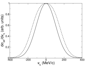
Figure 6: Normalized residue momentum distributions for the first (solid) and second (dashed) ²⁴Si(2⁺) states populated in $2n$ knockout from ²⁶Si. Though the same $sd$-shell two-nucleon configurations contribute to each state, their TNA result in distinct $L$ makeup and momentum distributions. The (FWHM) peak widths are are 250 and 330 MeV/c, respectively.

To consolidate our understanding of such sensitivity, we consider a further simplified example where a single configuration is expected to dominate. We consider the two configurations $[1d_{5/2}]^{2}$ and $[1d_{5/2},1d_{3/2}]$, both of which can contribute to 4⁺ states. States with such simple configurations may not be realized in ²⁴Si, since 4⁺ states in ²⁴Si are thought to be unbound, but the example will serve to illustrate the expected differences that may occur elsewhere in the $sd$-shell.

We construct the TNA as $C_{\alpha}^{41}=\sqrt{5/3}$, such that $N_{f}=1$, see Eq. (25), and the resulting $LS$-decomposition of strengths is given in Table 5. It is very clear that the $[1d_{5/2},1d_{3/2}]$ configuration weights $L=4$ significantly more strongly than does $[1d_{5/2}]^{2}$ and the expectation is a wider momentum distribution. As noted in Section II.1, in this case we would expect $L+S+T$=even contributions to be significantly suppressed due to the two-neutron antisymmetry and the similarity of the radial wave functions for the active spin-orbit partner orbitals. This is indeed the case, as demonstrated by the stripping cross sections of Table 5. The estimated strengths, $N_{f}^{LS}$, are seen to give a reasonable guide to the expected cross sections for these single configuration examples.

Table 5: $LS$-coupled strengths, $N_{f}^{LS}$, and $LS$ partial stripping cross sections for pure $[1d_{5/2}]^{2}$ and pure $[1d_{5/2},1d_{3/2}]$ two-neutron configurations populating $4^{+}$ final states in ²⁴Si. The cross section for $L=4$, $S=1$ is negligible, see text.

$\alpha$	$N_{f}^{31}$	$N_{f}^{40}$	$N_{f}^{41}$	$\sigma_{31}$	$\sigma_{40}$	$\sigma_{41}$
$[1d_{5/2}]^{2}$	0.8	0.2	0.0	0.23	0.09	0.00
$[1d_{5/2}][1d_{3/2}]$	0.1	0.4	0.5	0.06	0.35	0.00

The results of the calculations, shown in Fig. 7, confirm the differences in the momentum distributions expected from our simple consideration of the $N_{f}^{LS}$. Again, the specifics of the underlying structure predict considerable and observable differences in the expected residue momentum distributions.

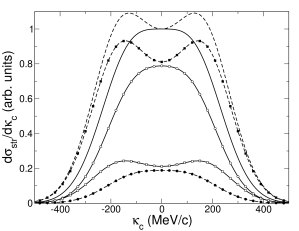
Figure 7: Examples of the projectile rest frame residue momentum distributions for $I=4$ states in the ²⁶Si($-2n$) reaction, arising from different neutron pair configurations. The solid lines and open points assume $[1d_{5/2}]^{2}$ neutron removal, the dashed lines and solid points assume $[1d_{5/2},1d_{3/2}]$ neutron removal. The full distributions are normalized to 1 at $\kappa_{c}=0$, with each contributing $L$ partial distribution scaled by the same factor. Circles show $L=3$, $S=1$ contributions and squares show $L=4$, $S=0$, with the total shown by the line. The different relative strengths of $L=3$ and $L=4$ for the two configurations generates significantly different ²⁴Si momentum distributions for states of the same $I$ (the dashed and solid curves).

IV.3 Cross shell: ⁵⁴Ti(-2p)

This ($T=1$) reaction, reported in Ref. GJB06 , demonstrated the potential for two-nucleon knockout to probe cross-shell proton excitations in neutron rich nuclei. In particular, a ⁵²Ca(3^-, 3.9 MeV) state was populated in two proton removal from ⁵⁴Ti(0⁺) on a ⁹Be target at 72 MeV per nucleon. Details of the eikonal $S$-matrices and nucleon radial wave functions can be found in Ref. GJB06 . Previous theoretical estimates for the 3^- state yield assumed pure $[1f_{7/2},2s_{1/2}]$ or $[1f_{7/2},1d_{3/2}]$ configurations, providing an estimated upper limit for the cross section to this state as an incoherent sum of these contributions.

Taking instead a coherent sum will give (a) a different total cross section, and (b) a different residue momentum distribution. Here we assess the expected sensitivity to the relative strengths and phases of these two configurations. We calculate the two-proton stripping cross sections and momentum distributions as a function of the TNA for $[1f_{7/2},1d_{3/2}]$ removal, $C_{fd}^{31}$, and for $[1f_{7/2},2s_{1/2}]$ removal, $C_{fs}^{31}$. For either of these pure configurations the stripping cross sections scale with $[C_{f\ell}^{IT}]^{2}$. To maintain an overall scaling when the configurations are mixed, the two amplitudes are adjusted such that

$$[C_{fs}^{31}]^{2}+[C_{fd}^{31}]^{2}=1\ ,$$ (33)

with $C_{fs}^{31}$ assumed positive. The total incoherent strength thus remains constant. We calculate the stripping cross sections for each contributing $LS$ combination and the full-width half-maximum (FWHM) for the residue momentum distributions. This is not the whole story for the momentum distribution – there are also subtle changes of shape beyond the nominal width – but this FWHM width provides a guide to the expected behavior. The resulting calculations are shown in Fig. 8. A few points follow immediately; the $[1f_{7/2},2s_{1/2}]$ configuration only contributes to the $L=3$ cross section, giving no interference with $L=2$ and $L=4$. So, these latter terms are simply proportional to $[C_{fd}^{31}]^{2}$ and are zero at the centre of the plot. The $L=4$ contributions are also generally weak and the overall width of the residue momentum distribution is largely determined by the relative strengths of the $L=2$ and $L=3$ contributions.

Both the cross section and FWHM of the momentum distribution show a strong sensitivity to the mixing of the two configurations; the cross section varies by a factor of two and the width of the momentum distribution by 25%. It is clear that the underlying structure and the relative strengths of the two-nucleon amplitudes are critical to determining both the removal cross section and the shape of the momentum distribution.

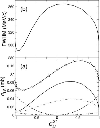
Figure 8: (a) Two-nucleon stripping cross sections and (b) the full-width at half-maximum of the residue momentum distribution when populating the ⁵²Ca(3^-, 3.9 MeV) state. These observables are shown as a function of the amplitude $C_{fd}^{31}$. The (positive) amplitude $C_{fs}^{31}$ of the second configuration is given by Eq. 33. The lower panel shows the partial cross sections with {$L,S$}, for the values {$2,1$} (dashed), {$3,0$} (solid), {$3,1$} (dotted) and {$4,1$} (dot-dashed). The total stripping cross section is shown by the solid line with open triangles).

Of interest are the extremes of the plot, with $|C_{fd}^{31}|\approx 1$. Here both the two-nucleon removal cross sections and momentum distribution widths are acutely sensitive to the small admixtures of the $[1f_{7/2},2s_{1/2}]$ configuration, but also strongly dependent on its sign. If the two amplitudes are of opposite phase then both the cross section and width decrease rapidly. Conversely, they increase rapidly if in phase. This is indicative of a sensitivity to small cross-shell admixtures in many cases.

We now contrast the impact parameter plane-projected two-nucleon joint probability distributions, for values of $C_{fd}^{31}=\pm\sqrt{2}/2$, in Fig. 9. The difference in this cross-shell case is now striking and it is clear that taking the amplitudes to be in phase (the +ve choice) enhances the two-nucleon spatial correlations, that then drives the significantly larger two-nucleon knockout cross section that is calculated and differences in the residue momentum distribution.

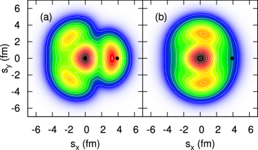
Figure 9: (Color online) Impact parameter plane-projected two-nucleon joint position probabilities, for $L=3$, $S=0$, for (a) $C_{fd}^{31}=\sqrt{2}/2$ and (b) $C_{fd}^{31}=-\sqrt{2}/2$ for the ⁵²Ca(3^-, 3.9 MeV) state populated in two-proton knockout form ⁵⁴Ti. The plot shows the probability distribution of nucleon 2 when nucleon 1 is positioned at the back circle. The color scale (white-blue-green-yellow-red-black) is the same for both plots. The source of the differences in the calculated cross sections (see Fig. 8) for these two choices of TNA is evident in the pair correlations manifest in these projected two-particle joint position probabilities Note the asymmetry at $\varphi_{12}=90^{\circ}$ (i.e. $s_{x}=0$), induced by mixing of different parity orbitals.

As is clear from Fig. 8, a precise measurement of the residue momentum distribution for this reaction would allow an estimate of the relative strengths and phases of the amplitudes of the two assumed active two-nucleon (cross-shell) configurations. The knockout cross sections themselves are also shown to depend strongly on the mixing. To date, analyses of two-nucleon knockout from exotic (asymmetric) systems have shown that the theoretical cross sections overestimate those measured experimentally by of a factor of about two, quantified as $R_{s}(2N)=\sigma_{expt}/\sigma_{theor}\approx 0.55$; see e.g. Ref. ToB06 . This suppression effect thus introduces an ambiguity in the absolute cross sections that is significant at the level of the differences being shown in Fig. 8. Such suppressions, of the cross sections predicted using the shell-model spectroscopy, may themselves be, at least in part, a manifestation of the use of TNA calculated in a truncated shell-model space and that exclude a large number of (small amplitude) cross-shell configurations. Based on the limited measurements available to date, there is no indication that the (missing) physics that drives the suppression of cross-section strength has implications for the shape of the residue momentum distribution. Additional, more accurate exclusive final state data are needed to assess these expectations further.

V Summary

We have discussed the momentum distributions of the heavy residues after two-nucleon knockout reactions using $LS$-coupling. The main factor determining the width of these momentum distributions is shown to be the transferred total orbital angular momenta $L$ of the two nucleons. We provide insight into the expected widths of momentum distributions from the removal of the nucleon pair from different configurations showing that information can be gained from and upon the strengths of the theoretical two nucleon amplitudes and the contributing $L$ they generate. The unambiguous observation of effects associated with specific pairs of nucleon orbitals may require transitions to final states that are relatively pure or simple configurations. Some illustrative examples were presented and discussed.

The conclusion of previous work - that the residue momentum distribution was simply characteristic of the final state spin - has been considered in further detail. It is true that, generally, higher spin final states will lead to wider residue momentum distributions, but that the details of the shell model two-nucleon overlap are important in understanding the details of the residue momentum distributions. Quantitative testing and confirmation of such sensitivity to the underlying structure will be essential for the exploitation of two-nucleon knockout methods and their extension for deformed nuclei.

The critical importance of configurations of different parity in enhancing pairing correlations is demonstrated by consideration of the angular correlations inherent in the two-nucleon density. Whilst discussed here in the context of two-nucleon removal reactions and enhancements of two-nucleon removal cross sections, such considerations, of large basis TNA, and the importance of small admixtures of different parity is entirely general. In the context of the suppression of shell model strength, previous studies with radioactive beams have demonstrated that the theoretical cross sections overestimate experiment by about a factor of two. It will be important to experimentally verify the influence of cross-shell excitations on structurally better-understood cases, such as for ¹²C, ¹⁶O and ⁴⁰Ca, to clarify the extent to which the necessary reductions may depend (in part) on the truncated model spaces used. It will also be important to further assess the importance of cross shell proton-excitations in studies of islands of inversion using the two-proton knockout methodology (see e.g. GAB07a ; AAB08 ; FRM10 ), where very strong reductions of two-proton knockout cross sections are observed.

Here our emphasis has been on light and medium mass projectiles. Another interesting example is the two-proton removal reaction from ²⁰⁸Pb; not only are there a large number of active orbitals, producing a plethora of states, but the majority of states are good two-proton hole configurations with minimal mixing.

The study of such reactions with odd-mass projectiles brings an added layer of complication with, typically, each final state being populated via several nucleon pair total angular momenta. The widths of the residue momentum distributions are then no longer simply related to a single final state spin. However, the underlying structure sensitivity discussed here may still yield characteristic widths for different final states in the same residue, somewhat independent of the final state spin.

- (1) P. G. Hansen, Phys. Rev. Lett. 77, 1016 (1996).
- (2) F. Barranco and E. Vigezzi, in Break-up of halo states induced by nuclear interactions, edited by R. A. Broglia and P. G. Hansen (World Scientific, 1998), p.217.
- (3) P. G. Hansen and J. A. Tostevin, Annu. Rev. Nucl. Part. Sci. 53, 219-261 (2003).
- (4) C. A. Bertulani and P.G. Hansen, Phys. Rev. C 70, 034609 (2004).
- (5) A. Gade, P. Adrich, D. Bazin, M. D. Bowen, B. A. Brown, C. M. Campbell, J. M. Cook, T. Glasmacher, P. G. Hansen, K. Hosier, S. McDaniel, D. McGlinchery, A. Obertelli, K. Siwek, L. A. Riley, J. A. Tostevin, and D. Weisshaar, Phys. Rev. C 77, 044306 (2008).
- (6) D. Bazin, B. A. Brown, C. M. Campbell, J. A. Church, D. C. Dinca, J. Enders, A. Gade, T. Glasmacher, P. G. Hansen, W. F. Mueller, H. Olliver, B. C. Perry, B. M. Sherrill, J. R.Terry, J. A. Tostevin, Phys. Rev. Lett. 91, 012501 (2003).
- (7) J. A. Tostevin, Eur. Phys. J. Spec. Top. 150, 67 (2007).
- (8) J. A. Tostevin, G. Podolyák, B.A. Brown and P.G. Hansen, Phys. Rev. C 70, 064602 (2004).
- (9) J. A. Tostevin, B.A. Brown, Phys. Rev. C 74, 064604 (2006).
- (10) E. C. Simpson and J. A. Tostevin, Phys. Rev. C 79, 024616 (2009).
- (11) E. C. Simpson, J.A. Tostevin, D. Bazin, and A. Gade, Phys. Rev. C 79, 064621 (2009).
- (12) E. C. Simpson, J. A. Tostevin, D. Bazin, B. A. Brown and A. Gade, Phys. Rev. Lett. 102, 132502 (2009).
- (13) P.G. Hansen and J.A. Tostevin, Annu. Rev. Nucl. Part. Sci. 53, 219 (2003).
- (14) C. A. Bertulani and C. De Conti, Phys. Rev. C 81, 064603 (2010).
- (15) N. C. Summers, J. S. Al-Khalili, and R. C. Johnson, Phys. Rev. C 66, 014614 (2002)
- (16) R. J. Glauber, in Lectures in Theoretical Physics, edited by W. E. Brittin and L. G. Dunham (Interscience Publishers, 1959), Vol. 1, p.315.
- (17) J. S. Al-Khalili, J.A. Tostevin and I.J. Thompson, Phys. Rev. C 54, 1843 (1996).
- (18) J. A. Tostevin, J. Phys. Conf. Ser. 49, 21 (2006).
- (19) G. F. Bertsch, R.A. Broglia and C. Riedel, Nucl. Phys. A91, 123 (1967).
- (20) W. T. Pinkston, Phys. Rev. C 29, 1123 (1984).
- (21) F. A. Janouch and R. J. Liotta, Phys. Rev. C 27, 896 (1983).
- (22) F. Catara, A. Insolia, E. Maglione and A. Vitturi , Phys. Rev. C 29, 1091 (1984).
- (23) F. Catara, A. Insolia, E. Maglione and A. Vitturi, Phys. Lett. B149, 41 (1984).
- (24) A. Insolia, R. J. Liotta and E. Maglione, J. Phys. G 15, 1249 (1989).
- (25) M. A. Tischler, A. Tonina, and G. G. Dussel, Phys. Rev. C 58, 2591 (1998).
- (26) B. A. Brown, Phys. Rev. C 58, 220 (1998).
- (27) B.A. Brown, A. Etchegoyen, N.S. Godwin, W.D.M. Rae, W.A. Richter, W.E. Ormand, E.K. Warburton, J.S. Winfield, L. Zhao, C. H. Zimmerman and H. Liu, Oxbash for Windows (MSU-NSCL report number 1289, 2004).
- (28) E. K. Warburton and B. A. Brown, Phys. Rev. C 46, 923 (1992)
- (29) B. A. Brown, P. G. Hansen, B. M. Sherrill and J. A. Tostevin, Phys. Rev. C 65, 061601 (2002).
- (30) J. A. Tostevin, P. Batham, G. Podolyák and I. J. Thompson, Nucl. Phys. A746, 166c-172c (2004).
- (31) E. C. Simpson and J. A. Tostevin (2010).
- (32) K. Yoneda, A. Obertelli, A. Gade, D. Bazin, B. A. Brown, C. M. Campbell, J. M. Cook, P. D. Cottle, A. D. Davies, D. -C.Dinca, T. Glasmacher, P. G. Hansen, T. Hoagland, K. W. Kemper, J. -L. Lecouey, W. F. Mueller, R. R. Reynolds, B. T. Roeder, J. R. Terry, J. A. Tostevin and H. Zwahlen, Phys. Rev. C 74, 021303(R) (2006).
- (33) B. H. Wildenthal, Prog. Part. Nucl. Phys, 11, 5 (1984).
- (34) B. A. Brown and W. A. Richter, Phys. Rev. C 74, 034315 (2006).
- (35) A. Gade, R.V.F. Janssens, D. Bazin, R. Broda, B. A. Brown, C. M. Campbell, M.P. Carpenter, J. M. Cook, A. N. Deacon, D.-C. Dinca, B. Fornal, S. J. Freeman, T. Glasmacher, P. G. Hansen, B. P. Kay, P. F. Mantica, W. F. Mueller, J. R. Terry, J. A. Tostevin, and S. Zhu, Phys. Rev. C 74, 021302 (2006).
- (36) A. Gade, P. Adrich, D. Bazin, M. D. Bowen, B. A. Brown, C. M. Campbell, J. M. Cook, S. Ettenauer, T. Glasmacher, K. W. Kemper, S. McDaniel, A. Obertelli, T. Otsuka, A. Ratkiewicz, K. Siwek, J. R. Terry, J. A. Tostevin, Y. Utsuno, and D. Weisshaar, Phys. Rev. Lett. 99, 072502 (2007).
- (37) P. Adrich, A. M. Amthor, D. Bazin, M. D. Bowen, B. A. Brown, C. M. Campbell, J. M. Cook, A. Gade, D. Galaviz, T. Glasmacher, S. McDaniel, D. Miller, A. Obertelli, Y. Shimbara, K. P. Siwek, J. A. Tostevin, and D. Weisshaar, Phys. Rev. C 77, 054306 (2008).
- (38) P. Fallon, E. Rodriguez-Vieitez, A.O. Macchiavelli, A. Gade, J. A. Tostevin, P.Adrich, D. Bazin, M. Bowen, C. M. Campbell, R. M. Clark, J. M. Cook, M. Cromaz, D.C. Dinca, T. Glasmacher, I. Y. Lee, S. McDaniel, W. F. Mueller, S. G. Prussin, A. Ratkiewicz, K. Siwek, J. R. Terry, D. Weisshaar, M. Wiedeking, K. Yoneda, B.A. Brown, T. Otsuka, Y. Utsuno, Phys. Rev. C 81, 041302(R) (2010).