Nonparametric inference procedure for percentiles of the random effects distribution in meta-analysis

Abstract

To investigate whether treating cancer patients with erythropoiesis-stimulating agents (ESAs) would increase the mortality risk, Bennett et al. [Journal of the American Medical Association 299 (2008) 914–924] conducted a meta-analysis with the data from 52 phase III trials comparing ESAs with placebo or standard of care. With a standard parametric random effects modeling approach, the study concluded that ESA administration was significantly associated with increased average mortality risk. In this article we present a simple nonparametric inference procedure for the distribution of the random effects. We re-analyzed the ESA mortality data with the new method. Our results about the center of the random effects distribution were markedly different from those reported by Bennett et al. Moreover, our procedure, which estimates the distribution of the random effects, as opposed to just a simple population average, suggests that the ESA may be beneficial to mortality for approximately a quarter of the study populations. This new meta-analysis technique can be implemented with study-level summary statistics. In contrast to existing methods for parametric random effects models, the validity of our proposal does not require the number of studies involved to be large. From the results of an extensive numerical study, we find that the new procedure performs well even with moderate individual study sample sizes.

, , and

t1Supported in part by NIH Grants R37 AI24643 and T32 AI007358. t2Supported in part by NIH Grant R01 HL089778. t3Supported in part by NIH Grants R37 AI24643 and U54 LM008748. t4Supported in part by NIH Grants R01 AI052817 and U54 LM008748.

1 Introduction

Conventional meta-analysis techniques have been utilized frequently to make inferences about a single parameter, for example, the center of the distribution of the random or fixed effects. Under the random effects model, the procedure for estimating the mean of the random effects proposed by DerSimonian and Laird (DL) (1986) is routinely used in practice. Their method utilizes a linear combination of study-specific point estimates with the weights depending on the within- and among-study variance estimates. This procedure is simple to implement and does not require patient-level data. Its validity, however, depends heavily on the individual study sample sizes and the number of studies [Brockwell and Gordon (2001), Bohning et al. (2002), Sidik and Jonkman (2007) and Viechtbauer (2007)]. In addition, this and other related methods for random effects models in meta-analysis do not provide inferences about the distribution function of the random effects. Estimation of this distribution function or its quantile counterpart provides valuable information for the complex risk-benefit decision on a new drug or device.

In a meta-analysis using the data from 52 phase III comparative trials (ESA vs. placebo or standard of care), Bennett et al. (2008) examined whether the erythropoiesis-stimulating agents (ESAs) for treating anemia of cancer patients would increase the patients’ risk of mortality. The point and 95% interval estimates of two-sample study-specific hazard ratio were presented in Figure 2 of Bennett et al. Bennett et al. (2008) concluded that administration of ESAs was significantly associated with increased mortality. Using the DL method, the resulting 95% confidence interval for the mean of the random hazard ratios (treated vs. untreated with ESA) across the studies was (1.01, 1.20). The lower bound of the interval is barely above $1$. Furthermore, it is known that the DL method can produce liberal confidence interval estimates, that is, the true coverage level tends to be smaller (sometimes substantially) than the nominal value [Emerson, Hoaglin and Mosteller (1993), Hardy and Thompson (1996), Brockwell and Gordon (2001, 2007) and Sidik and Jonkman (2002)]. Therefore, the interval estimates reported by Bennett et al. may be “too tight.” Moreover, from Figure 2 of Bennett et al., it appears that the study-specific hazard ratio estimates for 22 out of 52 trials are less than $1$, suggesting that even if the average hazard ratio is more than $1$, the ESA may not be harmful in all study populations. Last, since the DL method is based on a weighted average of hazard ratio estimates, the resulting interval estimates may be sensitive to outliers.

In this article we propose a simple inference procedure for the percentiles of the random effects distribution based on study-level data without assuming a parametric form of the distribution. We re-analyzed the mortality data reported in Bennett et al. (2008). The resulting 95% confidence interval for the median of the random hazard ratios was (0.94, 1.26). The 95% confidence interval for the lower quartile of the random hazard ratios was (0.70, 0.99), indicating that, in approximately a quarter of the study populations, ESA treatment may reduce mortality. In contrast to all existing methods, which can only handle inference for the center of the random effects distribution, the new proposal does not require the number of studies to be large. The new proposal is theoretically valid when the sample sizes of individual studies are large. Through an extensive numerical study, we find that the new method performs well even with moderate individual study sample sizes. On the other hand, the DL method tends to give liberal confidence interval estimators, that is, their coverage levels can be markedly smaller than the nominal value.

2 Interval estimates for percentiles of the random effects distribution

Consider a typical two-level hierarchical model. Let $\Pi^{\prime}=(\Theta,\Lambda^{\prime})$ be a row vector of random parameters, where $\Theta$ is a univariate parameter of interest and $\Lambda$ is a finite- or infinite-dimensional vector of nuisance parameters. Let $G(\cdot)$ be the continuous, completely unspecified distribution function of $\Theta.$ Given an unobservable realization $\Pi,$ a data set $X$ is generated. Let $\{\Pi_{k},X_{k}\},k=1,\ldots,K,$ be $K$ independent copies of $\{\Pi,X\}.$ The problem is how to make inferences, for instance, about the median $\mu$ of $G(\cdot)$ with $\{X_{k},k=1,\ldots,K\}.$ As an example, consider the case with $K$ $2\times 2$ tables and let $\Theta_{k}$ be the log-risk-ratio or risk difference for the $k$th table. Here, the nuisance parameter $\Lambda_{k}$ consists of the underlying event rate for the “control” group and the sample size for the $k$th study $n_{k}$.

If we can observe $\{\Theta_{k},k=1,\ldots,K\},$ a simple nonparametric estimator for $\mu$ is the sample median. Exact confidence intervals for $\mu$ can be obtained by inverting a sign test for the null hypothesis that the median is $\mu_{0}$. Under $H_{0}\dvtx\mu=\mu_{0}$, consider

$$T(\mu_{0})=\sum_{k=1}^{K}B_{k},$$ (1)

where $B_{k}=I(\Theta_{k}<\mu_{0})-I(\Theta_{k}>\mu_{0})$ and $I(\cdot)$ is the indicator function. The null distribution of $T(\mu_{0})$ can be generated by

$$T^{*}=\sum_{i=1}^{K}\Delta_{k}\qquad\mbox{where }\Delta_{k}=\cases{\hskip 8.4pt1,&\quad with probability 0.5,\cr-1,&\quad otherwise.}$$ (2)

Suppose that, given $\Pi_{k},$ $\hat{\Theta}_{k}$ is a consistent estimator for $\Theta_{k}$ based on the data $X_{k}$. To test $H_{0}$, one may replace $\Theta_{k}$ in (1) with $\hat{\Theta}_{k}.$ This results in the test statistic

$$\tilde{T}(\mu_{0})=\sum_{k=1}^{K}\hat{B}_{k}=\sum_{k=1}^{K}\{I(\hat{\Theta}_{k}<\mu_{0})-I(\hat{\Theta}_{k}>\mu_{0})\}.$$ (3)

When the sample size $n_{k}$ for each individual study is large, we can make inferences about the median by comparing the observed value of (3) to the distribution of (2).

Now, the test based on (3) does not take into account the precision of the estimator $\hat{\Theta}_{k}.$ It gives equal weight to each individual study. For the $k$th study, suppose that the variance $\hat{\sigma}_{k}^{2}$ of $\hat{\Theta}_{k}$ is large relative to the distance between $\Theta_{k}$ and $\mu_{0}.$ Then the likelihood of the unobservable $\Theta_{k}<\mu_{0}$ can be quite close to $1/2$ (like tossing a fair coin). Therefore, the noise generated from such an unstable $\hat{B}_{k}$ may well outweigh its added value to the power of the test based on $\tilde{T}(\mu_{0}).$ On the other hand, if $\hat{\sigma}^{2}_{k}$ is small and $\hat{\Theta}_{k}<\mu_{0}$, the likelihood of $\Theta_{k}<\mu_{0}$ would be closer to 1.

This motivates us to modify test statistic (3) by putting weight $w_{k}$ on $\hat{B}_{k}$. Here, $w_{k}$ is a measure of likelihood of the event $\Theta_{k}<\mu_{0},$ for example, the observed coverage level of the interval $(-\infty,\mu_{0})$ for the realized $\Theta_{k}$. When the individual study size $n_{k}$ is large, and the distribution of $\hat{\Theta}_{k}$ conditional on $\Pi_{k}$ is approximately normal with mean $\Theta_{k}$ and variance $\hat{\sigma}_{k}^{2},$ where $n_{k}\hat{\sigma}_{k}^{2}$ converges to a constant, this coverage level is approximately $\Phi((\mu_{0}-\hat{\Theta}_{k})/\hat{\sigma}_{k})$, where $\Phi$ is the distribution function of the standard normal. Let the resulting test statistic be

$$\hat{T}(\mu_{0})=\sum_{k=1}^{K}\bigl{|}\Phi\bigl{(}(\mu_{0}-\hat{\Theta}_{k})/\hat{\sigma}_{k}\bigr{)}-1/2\bigr{|}\hat{B}_{k}.$$ (4)

In the Appendix we show that, in probability, for any given $\mu,$

$$\bigl{|}\Phi\bigl{(}(\mu-\hat{\Theta}_{k})/\hat{\sigma}_{k}\bigr{)}-1/2\bigr{|}\hat{B}_{k}-B_{k}/2\rightarrow 0\qquad\mbox{as }n_{k}\rightarrow\infty.$$ (5)

It follows that, for fixed $K,$ for large $n_{k},k=1,\ldots,K,$ the distribution of $\hat{T}(\mu_{0})$ approximates that of $T(\mu_{0}).$ This approximation, however, is rather discrete; and for moderate sample sizes, the resulting confidence intervals for $\mu$ do not have adequate coverage levels in our numerical study (Section 4). An alternative way to generate an approximation to the null distribution of $\hat{T}(\mu_{0})$ is to use

$$\hat{T}^{*}(\mu_{0})=\sum_{k=1}^{K}\bigl{|}\Phi\bigl{(}(\mu_{0}-\hat{\Theta}_{k})/\hat{\sigma}_{k}\bigr{)}-1/2\bigr{|}\Delta_{k}.$$ (6)

Here, the $\Delta_{k}$’s are the only random quantities and are analogous to the random multipliers used in the wild bootstrap [Wu (1986)]. The weight from the $k$th study is multiplied by $\Delta_{k}$, which is $1$ or $-1$ with probability 0.5 and is generated by the analyst independently of the observed data. In the Appendix, we also justify the asymptotic validity of the test based on (4) and (6). Confidence intervals for $\mu$ can be obtained by inverting this test. In contrast to other methods, the new proposal does not require the number of studies ($K$) to be large. In Section 4 we show empirically that the new interval estimation procedure performs well even when the sample sizes $(n_{k})$ are not large.

The above proposal can be generalized easily to make inferences about certain percentiles of the distribution $G(\cdot)$. Specifically, let us hypothesize that the 100$p$th percentile is $\mu_{0}.$ As for the median, define $B_{k}=I(\Theta_{k}<\mu_{0})-I(\Theta_{k}>\mu_{0}),$ and obtain $\hat{B}_{k}$ by replacing $\Theta_{k}$ in $B_{k}$ with $\hat{\Theta}_{k}.$ The test statistic is given by

$$\hat{T}_{p}(\mu_{0})=\sum_{k=1}^{K}\bigl{|}\Phi\bigl{(}(\mu_{0}-\hat{\Theta}_{k})/\hat{\sigma}_{k}\bigr{)}-1/2\bigr{|}\hat{B}_{k},$$ (7)

and the null distribution is generated by

$$\hat{T}_{p}^{*}(\mu_{0})=\sum_{k=1}^{K}\bigl{|}\Phi\bigl{(}(\mu_{0}-\hat{\Theta}_{k})/\hat{\sigma}_{k}\bigr{)}-1/2\bigr{|}\Delta_{k},$$ (8)

where $\Delta_{k}=1$ with probability $p$ and $=-1$ with probability $1-p.$ Let the resulting test statistic corresponding to (3) be denoted by $\tilde{T}_{p}(\mu_{0})$. Confidence intervals for the 100$p$th percentile can then be obtained by inverting the conditional test accordingly.

3 Safety meta-analysis of erythropoiesis-stimulating agents

We re-analyzed the data reported in Bennett et al. (2008) using the new proposal. Here $K=52,$ and for the $k$th study, $\Theta_{k}$ was the log-hazard ratio and $\hat{\Theta}_{k}$ was its estimate. Since the patient-level data were not available, we approximated the standard error estimate of $\hat{\Theta}_{k}$ by one-fourth of the reported length of the 95% confidence interval (converted to the log-scale). The 95% confidence interval for the median of the distribution of the random hazard ratio $(\exp(\Theta))$ was $(0.94,1.21)$ based on the test statistic $\hat{T}(\cdot)$ and (6). The corresponding interval based on the indicator functions $\{I(\hat{\Theta}_{k}<\mu)\}$ via $\tilde{T}(\cdot)$ was $(0.90,1.26),$ which was wider than the above interval. The 95% confidence interval for the $mean$ of the random effects distribution reported in Bennett et al. (2008) using the DL method was $(1.01,1.20)$. In the next section we show that the empirical coverage levels of the DL method can be substantially lower than their nominal counterparts even when the number of studies is not that small (say, $K=40$).

The 95% intervals for the $25$th and $75$th percentiles based on (7) and (8) were (0.70, 0.99) and (1.18, 1.48), respectively. The counterparts based on $\tilde{T}_{p}(\cdot)$ were (0.49, 0.93) and (1.25, 1.72). Again, the intervals based on $\hat{T}_{p}(\cdot)$ were shorter than those with $\tilde{T}_{p}(\cdot).$ Note that the upper bound of the 95% interval for the 25th percentile was smaller than 1, which suggested that, approximately, for a quarter of the study populations, their average hazard ratios for the ESA versus the control were most likely less than one. That is, on average, the patients in these study populations may benefit from taking ESA with respect to mortality.

Further investigation to identify characteristics of these trials would be informative for identifying future cancer patients who would benefit from the ESAs through reduction of blood cell transfusions and improved quality of life. On the other hand, it is crucial to identify future patients who would have unacceptable toxicity risks.

Bennett et al. (2008) also separately evaluated cancer-related anemia with six studies (see the top portion of Figure 2 in Bennett et al.) and investigated whether ESAs would increase the risk of a venous thromboembolism event (VTE) from 38 comparative phase III trials. The results obtained using the new proposal are reported in the supplemental article [Wang et al. (2009)].

4 Numerical studies to evaluate performance of the new proposal

We conducted extensive numerical studies to examine the performance of the proposed interval estimation procedure for the percentiles of the random effects model under various practical settings. The existing random effects methods for meta-analysis have focused on making inferences about the mean of the random effects distribution. To the best of our knowledge, no other methods address the same issue as our proposed procedure does. Our numerical studies included the DL interval estimation method, the method proposed by Sidik and Jonkman (2002) (SJ), and the one based on $\tilde{T}(\cdot)$ for comparisons. We considered cases with binary or continuous responses, various symmetric or asymmetric random effects distributions, and a wide range of study sample sizes and number of studies. From the results of our numerical investigation, we find that the new proposal performs well with respect to the confidence interval coverage level and length. The DL (or SJ) method tends to be liberal, that is, the empirical coverage levels can be markedly lower than their nominal counterparts. The procedure based on the test statistic $\tilde{T}(\cdot)$ produces confidence intervals whose average lengths are uniformly wider than those with our method. For percentiles other than the median, the method based on $\tilde{T}_{p}(\cdot)$ may have under-coverage.

Specifically, in our numerical studies, we first considered meta-analysis for multiple $2\times 2$ tables under settings similar to the meta-analysis of VTE rates in Figure 3 of Bennett et al. (2008). There are 41 studies listed and the raw data are available for 40 studies. We let $\Theta_{k}=\log(P_{1k}/P_{0k})$ be the log-relative risk for the $k$th study, where $P_{1k}$ and $P_{0k}$ are the underlying event rates for the ESA and control groups, respectively. We then assumed that the random vectors $(\operatorname{logit}(P_{0k}),\operatorname{logit}(P_{1k}))^{\prime}$ were a random sample of size $K$ from a bivariate normal, whose mean $\eta$ and variance–covariance matrix $\Sigma$ were estimated by their sample counterparts via the observed rates in Figure 3 of Bennett et al. (2008). We used the conventional 0.5 continuity correction for studies with zero cells. The resulting sample means and variance–covariance matrix are $(-3.56,-2.86)^{\prime}$ and $\left({0.90\atop 0.62}\enskip{0.62\atop 1.10}\right),$ respectively. The density of $\Theta$ is given in Figure 1 [panel (a)], which appears to be quite symmetric. For each realization $\{(P_{0k},P_{1k})^{\prime},k=1,\ldots,K\},$ we generated the corresponding set of $2\times 2$ tables. We then used DL, SJ, $\hat{T}(\cdot)$ and $\tilde{T}(\cdot)$ to construct 95% confidence intervals for the median of the distribution of $\Theta.$ For each realized data set, we excluded studies with 0–0 cells (that is, no events occurred in either group), and used the 0.5 continuity correction for studies with one zero cell. The average empirical coverage levels and the median interval lengths were obtained from 2000 realized data sets.

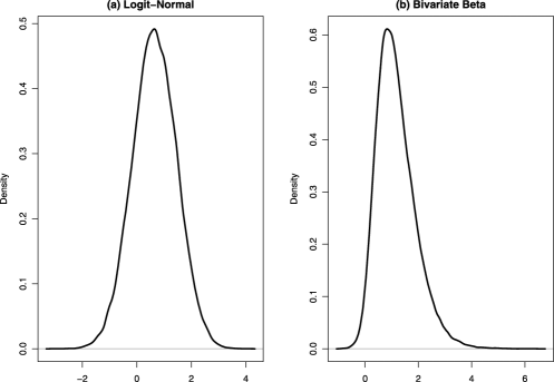
Figure 1: The true density functions for the random log-relative-risk parameter for the simulation study.

Table 1: Empirical coverage levels (ECL) and median lengths (ML) of 95% interval estimates for median based on DerSimonian–Laird (DL), Sidik and Jonkman (SJ), $\hat{T}(\cdot)$ and $\tilde{T}(\cdot)$ with a bivariate logit-normal or a bivariate beta distribution for the two underlying random event rates

Number of studies, $\bolds{K}$	DL		SJ		$\bolds{\hat{T}(\cdot)}$		$\bolds{\tilde{T}(\cdot)}$
	ECL	ML	ECL	ML	ECL	ML	ECL	ML
	Bivariate logit-normal
$40$	86%	0.62	88%	0.65	94%	0.72	95%	0.90
$30$	88%	0.71	91%	0.75	94%	0.83	95%	1.03
$20$	88%	0.85	91%	0.90	94%	1.00	95%	1.23
$10$	88%	1.18	94%	1.36	95%	1.54	97%	2.15
$6$	91%	1.57	97%	2.06	95%	2.29	97%	2.89
	Bivariate beta
$40$	87%	0.40	89%	0.42	95%	0.52	96%	0.65
$30$	88%	0.46	90%	0.48	95%	0.61	96%	0.75
$20$	90%	0.55	92%	0.59	96%	0.75	96%	0.91
$10$	91%	0.76	93%	0.89	96%	1.10	98%	1.56
$6$	88%	1.00	94%	1.30	95%	1.58	97%	2.10

Under the same setting, we repeated this process with $K=40$, $30$, $20$, $10$ and $6$. For each $K,$ the sample sizes came from the first $K$ studies listed in Figure 3 of Bennett et al. (2008). The results are summarized in Table 1 (top half). The average coverage levels for our proposed method, $\hat{T}(\cdot)$, range from 0.94 to 0.95. On the other hand, the average empirical coverage level can be as low as 0.86 for the DL method, and 0.88 for the SJ method. The median lengths of the intervals obtained via $\hat{T}(\cdot)$ are uniformly smaller than those of the procedure using $\tilde{T}(\cdot).$ In Table 2 (top half), we report the results for the $25$th and $75$th percentiles. Again our proposal behaves well, but the one with $\tilde{T}_{p}(\cdot)$ may not have the correct coverage level.

We also considered rather asymmetric random effects distributions. For example, we considered a bivariate beta distribution for $\{(P_{0k},P_{1k})^{\prime}$, $k=1,\ldots,40\}$ via three independent gamma random variables with a common unit scale parameter and shape parameters of $2$, $8$ and $10$, respectively [Olkin and Liu (2003)]. The resulting density function of the random parameter $\Theta,$ the log-relative risk, is given in Figure 1 [panel (b)]. Under the same setting as the previous simulation, the results are reported in the bottom half portions of Tables 1 and 2. Again, the new procedure performs well. The DL (or SJ) method still has coverage problems. Although the DL method produces confidence interval estimates for the mean of $G(\cdot)$, not the median, its empirical coverage for the mean was also lower than the nominal 95%. For example, when $K=40$, the coverage of DL for the mean was only 64%.

Table 2: Empirical coverage levels (ECL) and median lengths (ML) of 95% confidence intervals for the 25th and 75th percentiles based on $\hat{T}_{p}(\cdot)$ and $\tilde{T}_{p}(\cdot)$ with a bivariate logit-normal or a bivariate beta distribution for the two underlying random event rates

	25th percentile				75 percentile
Number of studies, $\bolds{K}$	$\bolds{\hat{T}_{p}(\cdot)}$		$\bolds{\tilde{T}_{p}(\cdot)}$		$\bolds{\hat{T}_{p}(\cdot)}$		$\bolds{\tilde{T}_{p}(\cdot)}$
	ECL	ML	ECL	ML	ECL	ML	ECL	ML
	Bivariate logit-normal
$40$	95%	0.86	86%	1.16	95%	0.81	92%	0.92
$35$	96%	0.91	88%	1.21	96%	0.86	90%	1.02
$30$	96%	1.00	90%	1.37	96%	0.94	91%	1.12
$25$	96%	1.12	90%	1.49	97%	1.06	92%	1.23
$20$	96%	1.24	92%	1.52	97%	1.16	92%	1.32
	Bivariate beta
$40$	96%	0.48	93%	0.55	96%	0.73	92%	0.96
$35$	96%	0.52	95%	0.61	96%	0.78	93%	1.04
$30$	95%	0.56	94%	0.64	96%	0.85	93%	1.07
$25$	96%	0.62	93%	0.65	96%	0.94	92%	1.10
$20$	96%	0.72	95%	0.80	96%	1.37	95%	1.37

Although our method assumes that the random effects distribution is continuous, we also considered cases with fixed effects models in our numerical study. For example, we let $(P_{0k},P_{1k})=(0.1,0.2),k=1,\ldots,K.$ The results are summarized in Table 3. For this case, the DL method has correct coverage level for most scenarios under which our interval estimation procedure is comparable with the DL method with respect to efficiency, which is reflected in the interval length. We also studied the performance of our method for $\Theta_{k}=P_{1k}-P_{0k},$ the risk difference for the $k$th study. The results were very similar to those for the relative risk.

Table 3: Empirical coverage levels (ECL) and median lengths (ML) of 95% interval estimates for median based on DerSimonian–Laird (DL), $\hat{T}(\cdot)$ and $\tilde{T}(\cdot)$ under a fixed effect model (the underlying event rates are 0.1 and 0.2)

Number of studies, $\bolds{K}$	DL		$\bolds{\hat{T}(\cdot)}$		$\bolds{\tilde{T}(\cdot)}$
	ECL	ML	ECL	ML	ECL	ML
$40$	92%	0.24	95%	0.27	96%	0.35
$30$	94%	0.26	95%	0.30	96%	0.39
$20$	95%	0.30	95%	0.35	97%	0.45
$10$	97%	0.47	96%	0.57	98%	0.84
$6$	96%	0.75	95%	1.03	97%	1.34

Our numerical studies with continuous responses yielded similar results. We summarize the study settings and the results in the supplemental article [Wang et al. (2009)]. We expect similar results for censored time to event observations, where hazard ratios are used for treatment effect measurements.

5 Discussion

In this article we present a simple nonparametric interval estimation procedure for percentiles of the random effects distribution. Random effects meta-analysis is frequently employed in medical research. However, the validity of the most popular method (DL) and its variations [Hardy and Thompson (1996), Biggerstaff and Tweedie (1997), Hartung (1999), Hartung and Knapp (2001a, 2001b) and DerSimonian and Kacker (2007)] is not clear when the number of studies is not large or the parametric assumption for the random effects is violated. An excellent review on meta-analysis with the random effects model is given by Sutton and Higgins (2008). In contrast to previous methods, our proposal does not require the number of studies to be large. The new proposal is valid provided the individual study sample sizes are large.

In addition, if the random effects distribution is symmetric and the $exact$ distribution of $\hat{\Theta}_{k},$ $k=1,\ldots,K,$ conditional on $\Pi_{k}$, is symmetric around the unknown fixed realized $\Theta_{k},$ it is easy to show that the resulting interval estimators based on $\hat{T}(\cdot)$ for the median (or mean) are valid without requiring the sizes of the individual studies or the number of studies to be large. For instance, under the usual two-sample location shift model with continuous response variable, let $\Theta$ be the location shift parameter of interest. Then, the two-sample rank estimator $\hat{\Theta}$ is symmetric around $\Theta$ under rather mild conditions [Lehmann (1975), page 86]. If the unspecified random effects distribution is symmetric around $\mu,$ one can use our procedure to obtain exact confidence intervals for $\mu.$ To examine the performance of the method in this setting, we conducted a simulation study, described in detail in the supplemental article [Wang et al. (2009)].

The proposed procedure can be implemented with study level summary statistics. When patient level data are available, various novel procedures have been studied for mixed effects regression models for continuous, discrete or censored event time observations [Laird and Ware (1982), Hougaard (1995), Hogan and Laird (1997), Henderson, Diggle and Dobson (2000), Lam, Lee and Leung (2002), Nelder, Lee and Pawitan (2006), Cai, Cheng and Wei (2002), Zeng and Lin (2007) and Zeng, Lin and Lin (2008)]. To the best of our knowledge, all of the existing asymptotic procedures for mixed effects models assume that the number of studies is large.

In the current practice of meta-analysis, inferences are made only for the “center” of the random effects distribution. A conclusion on the risk or benefit from an intervention based solely on an estimated center of the random effects distribution provides limited information and is usually not sufficient. If the number of studies involved is not small, we highly recommend estimating this distribution or its percentiles as proposed in this article.

Under the fixed effects model, this distribution has a single unknown mass point. The standard estimation procedure for such a fixed parameter value utilizes a weighted average of study-specific point estimates. For analyzing multiple $2\times 2$ tables, the most commonly used procedures are the Mantel–Haenszel [Mantel and Haenszel (1959)] and Peto methods [Yusuf et al. (1985)]. These methods are valid when the number of studies and each individual study sample size are large. Moreover, when the event rate is small, these standard methods may not perform well. For the fixed effects model, Tian et al. (2009) proposed a general exact interval estimation procedure that combines study-specific exact confidence intervals instead of point estimates. If the fixed effects model is approximately correct, the existing interval procedures for the common parameter value $\mu$ may be more efficient than those developed under the random effects model. The standard heterogeneity tests generally do not have the power to detect violations of the fixed effects modeling assumption. Therefore, in practice, sensitivity analyses with both random and fixed effects models are highly recommended.

Appendix: Justification for the conditional test $\hat{T}(\cdot)$ based on the approximation generated by $\hat{T}^{*}(\cdot)$

Let $D_{k}=|\Phi((\mu-\hat{\Theta}_{k})/\hat{\sigma}_{k})-1/2|\hat{B}_{k}-B_{k}/2$. We show that $D_{k}$ goes to 0, in probability, as $n_{k}\rightarrow\infty.$ Here, the probability is generated by the random element $(X_{k},\Pi_{k}).$ For any fixed positive constant $c,$ first we show that $\operatorname{pr}(|D_{k}|\geq c|\Pi_{k})\rightarrow 0$ for any given $\Pi_{k}$ with $\Theta_{k}\neq\mu.$ To this end, consider two cases. First, if $\Theta_{k}<\mu,$ then conditional on $\Pi_{k},$

$$|D_{k}|=\bigl{|}\Phi\bigl{(}(\mu-\hat{\Theta}_{k})/\hat{\sigma}_{k}\bigr{)}-1\bigr{|}=1-\Phi\bigl{(}(\mu-\Theta_{k})/\hat{\sigma}_{k}+(\Theta_{k}-\hat{\Theta}_{k})/\hat{\sigma}_{k}\bigr{)}.$$

As $n_{k}\to\infty$, $(\mu-\Theta_{k})/\hat{\sigma}_{k}\rightarrow\infty$ in probability, and $(\Theta_{k}-\hat{\Theta}_{k})/\hat{\sigma}_{k}\rightarrow N(0,1)$ in distribution. Therefore, for any $c>0$, we can find $N$ such that, when $n_{k}>N$, $\operatorname{pr}((\mu-\Theta_{k})/\hat{\sigma}_{k}+(\Theta_{k}-\hat{\Theta}_{k})/\hat{\sigma}_{k}\leq\Phi^{-1}(1-c))<c,$ which is equivalent to $\operatorname{pr}(\Phi((\mu-\hat{\Theta}_{k})/\hat{\sigma}_{k})<1-c)=\operatorname{pr}(|D_{k}|\geq c)<c.$ Therefore, $\operatorname{pr}(|D_{k}|\geq c\mid\Pi_{k})\rightarrow 0$. Similarly, if $\Theta_{k}>\mu$, we can show that $\operatorname{pr}(|D_{k}|\geq c\mid\Pi_{k})\rightarrow 0$ as $n_{k}\rightarrow\infty.$ Therefore, $\operatorname{pr}(|D_{k}|\geq c\mid\Pi_{k})\rightarrow 0$ for any $\Pi_{k}$ such that $\Theta_{k}\neq\mu.$

This, coupled with the fact that $G(\cdot)$ is continuous, implies that $\operatorname{pr}(|D_{k}|\geq c)=\mbox{E}_{\Pi_{k}}\{\operatorname{pr}(|D_{k}|\geq c\mid\Pi_{k})\}\rightarrow 0$ for any $c$ by the dominated convergence theorem. Therefore, $D_{k}\to 0$ in probability as $n_{k}\rightarrow\infty.$ It follows that $|\hat{T}(\mu)-\sum_{k=1}^{K}B_{k}/2|\to 0,$ in probability, as $\min\{n_{1},\ldots,n_{K}\}\rightarrow\infty.$

Similarly, since

$$\bigl{|}\bigl{|}\Phi\bigl{(}(\mu-\hat{\Theta}_{k})/\hat{\sigma}_{k}\bigr{)}-1/2\bigr{|}\Delta_{k}-|I(\Theta_{k}<\mu)-1/2|\Delta_{k}\bigr{|}\leq|D_{k}|,$$

one can show that $\hat{T}^{*}(\mu)-\sum_{k=1}^{K}|I(\Theta_{k}<\mu)-1/2|\Delta_{k}\to 0,$ in probability, as $\min\{n_{1},\ldots,n_{K}\}\rightarrow\infty,$ where

$$\Delta_{k}=\cases{\hskip 8.4pt1,&\quad$\mbox{with probability }p,$\cr-1,&\quad$\mbox{with probability }1-p,$}$$

for the 100$p$th percentile and is independent of the data. Therefore, for any $t$ and positive $c$,

$$\operatorname{pr}_{\{(X_{k},\Pi_{k})_{k=1,\ldots,K}\}}\Biggl{(}\Biggl{|}\operatorname{pr}\bigl{(}\hat{T}^{*}(\mu)\leq t|(X_{k},\Pi_{k})_{k=1,\ldots,K}\bigr{)}-\operatorname{pr}\Biggl{(}\sum_{k=1}^{K}\Delta_{k}/2\leq t\Biggr{)}\Biggr{|}\geq c\Biggr{)}$$

$$\qquad\leq c,$$

when $\min\{n_{1},\ldots,n_{K}\}$ is large. This, coupled with the fact that $\sum_{k=1}^{K}B_{k}/2\sim\sum_{k=1}^{K}\Delta_{k}/2$ under the null hypothesis that the 100$p$th percentile of $\Theta_{k}$ is $\mu$, implies that one can approximate the null distribution of $\hat{T}(\mu)$ by the distribution of $\hat{T}^{*}(\mu)$ conditional on the observed data.

References

- (1) Bennett, C. L., Silver, S. M., Djulbegovic, B., Samaras, A. T., Blau, C. A., Gleason, K. J., Barnato, S. E., Elverman, K. M., Courtney, D. M., McKoy, J. M., Edwards, B. J., Tigue, C. C., Raisch, D. W., Yarnold, P. R., Dorr, D. A., Kuzel, T. M., Tallman, M. S., Trifilio, S. M., West, D. P., Lai, S. Y. and Henke, M. (2008). Venous thromboembolism and mortality associated with recombinant Erythropoietin and Darbepoetin administration for the treatment of cancer-associated anemia. Journal of the American Medical Association 299 914–924.
- (2) Biggerstaff, B. J. and Tweedie, R. L. (1997). Incorporating variability in estimates of heterogeneity in the random effects model in meta-analysis. Statistics in Medicine 16 753–768.
- (3) Bohning, D., Malzahn, U., Dietz, E. and Schlattmann, P. (2002). Some general points in estimating heterogeneity variance with the DerSimonian–Laird estimator. Biostatistics 3 445–457.
- (4) Brockwell, S. E. and Gordon, I. R. (2001). A comparison of statistical methods for meta-analysis. Statistics in Medicine 20 825–840.
- (5) Brockwell, S. E. and Gordon, I. R. (2007). A simple method for inference on an overall effect in meta-analysis. Statistics in Medicine 26 4531–4543. \MR2411886
- (6) Cai, T., Cheng, S. C. and Wei, L. J. (2002). Semiparametric mixed-effects models for clustered failure time data. J. Amer. Statist. Assoc. 97 514–522. \MR1941468
- (7) DerSimonian, R. and Laird, N. M. (1986). Meta-analysis in clinical trials. Controlled Clinical Trials 7 177–188.
- (8) DerSimonian, R. and Kacker, R. (2007). Random-effects model for meta-analysis of clinical trials: An update. Contemporary Clinical Trials 28 105–114.
- (9) Emerson, J. D., Hoaglin, D. C. and Mosteller, F. (1993). A modified random-effect procedure for combining risk difference in sets of tables from clinical trials. Journal of the Italian Statistical Society 2 269–290.
- (10) Hardy, R. J. and Thompson, S. G. (1996). A likelihood approach to meta-analysis with random effects. Statistics in Medicine 15 619–629.
- (11) Hartung, J. (1999). An alternative method for meta-analysis. Biometrical Journal 41 901–916. \MR1747520
- (12) Hartung, J. and Knapp, G. (2001a). A refined method for the meta-analysis of controlled clinical trials with binary outcome. Statistics in Medicine 20 3875–3889.
- (13) Hartung, J. and Knapp, G. (2001b). On tests of the overall treatment effect in meta-analysis with normally distributed responses. Statistics in Medicine 20 1771–1782.
- (14) Henderson, R., Diggle, P. and Dobson, A. (2000). Joint modelling of longitudinal measurements and event time data. Biostatistics 1 465–480.
- (15) Hogan, J. W. and Laird, N. M. (1997). Mixture models for the joint distribution of repeated measures and event times. Statistics in Medicine 16 239–257.
- (16) Hougaard, P. (1995). Frailty models for survival data. Lifetime Data Anal. 1 255–273.
- (17) Laird, N. M. and Ware, J. H. (1982). Random effects models for longitudinal data. Biometrics 38 963–974.
- (18) Lam, K. F., Lee, Y. W. and Leung, T. L. (2002). Modeling multivariate survival data by a semiparametric random effects proportional odds model. Biometrics 58 316–323. \MR1908171
- (19) Lehmann, E.L. (1975). Nonparametrics: Statistical Methods Based on Ranks. Holden-Day, San Francisco. \MR0395032
- (20) Mantel, N. and Haenszel, W. (1959). Statistical aspects of the analysis of data from retrospective studies of disease. Journal of National Cancer Institution 22 719–748.
- (21) Nelder, J. A., Lee, Y. and Pawitan, Y. (2006). Generalized Linear Models with Random Effects: A Unified Approach via H-Likelihood. Chapman & Hall, London. \MR2259540
- (22) Olkin, I. and Liu, R. (2003). A bivariate Beta distribution. Statist. Probab. Lett. 62 407–412. \MR1973316
- (23) Sidik, K. and Jonkman, J. N. (2002). A simple confidence interval for meta-analysis. Statistics in Medicine 21 3153–3159.
- (24) Sidik, K. and Jonkman, J. N. (2007). A comparison of heterogeneity variance estimators in combining results of studies. Statistics in Medicine 26 1964–1981. \MR2364286
- (25) Sutton, A. J. and Higgins, J. P. T. (2008). Recent developments in meta-analysis. Statistics in Medicine 27 625–650. \MR2418504
- (26) Tian, L., Cai, T., Pfeffer, M. A., Piankov, N., Cremieux, P. and Wei, L. J. (2009). Exact and efficient inference procedure for meta-analysis and its application to the analysis of independent tables with all available data but without artificial continuity correction. Biostatistics 10 275–281.
- (27) Viechtbauer, W. (2007). Confidence intervals for the amount of heterogeneity in meta-analysis. Statistics in Medicine 26 37–52. \MR2312698
- (28) Wang, R., Tian, L., Cai, T. and Wei, L. J. (2009). Supplement to “Nonparametric inference procedure for percentiles of the random effects distribution in meta analysis.” DOI: 10.1214/09-AOAS280SUPP.
- (29) Wu, C. F. J. (1986). Jackknife, bootstrap, and other resampling methods in regression analysis. Ann. Statist. 14 1261–1295. \MR0868303
- (30) Yusuf, S., Peto, R., Lewis, J., Collins, R. and Sleight, P. (1985). Beta blockade during and after myocardial infarction: An overview of the randomised trials. Progress in Cardiovascular Diseases 27 335–371.
- (31) Zeng, D. and Lin, D. Y. (2007). Maximum likelihood estimation in semiparametric regression models with censored data. J. R. Statist. Soc. Ser. B Stat. Methodol. 69 507–564. \MR2370068
- (32) Zeng, D., Lin, D. Y. and Lin, X. (2008). Semiparametric transformation models with random effects for clustered failure time data. Statist. Sinica 18 355–377. \MR2384992