Constraining halo occupation properties of X-ray AGNs using
clustering
of Chandra sources in the Boötes survey region
Abstract
We present one of the most precise measurement to date of the spatial clustering of X-ray selected AGNs using a sample derived from the Chandra X-ray Observatory survey in the Boötes field. The real-space two-point correlation function over a redshift interval from to is well described by the power law, , for comoving separations Mpc. We find and consistent with no redshift trend within the sample (varying between Mpc for and Mpc for ). Further, we are able to measure the projections of the two-point correlation function both on the sky plane and in the line of sight. We use these measurements to show that the Chandra/Boötes AGNs are predominantly located at the centers of dark matter halos with the circular velocity km s-1 or , and tend to avoid satellite galaxies in halos of this or higher mass. The halo occupation properties inferred from the clustering properties of Chandra/Boötes AGNs — the mass scale of the parent dark matter halos, the lack of significant redshift evolution of the clustering length, and the low satellite fraction — are broadly consistent with the Hopkins et al. (2006) scenario of quasar activity triggered by mergers of similarly-sized galaxies.
1. Introduction
Direct observations of host galaxies of high-redshift active galactic nuclei are hard or impossible with the current instrumentation, except for highly obscured or low-luminosity objects. Hence, studies of the AGN clustering properties are a unique source of information on the AGN hosts and their environment. At low redshifts, the supermassive black holes exist at the centers of most low-redshift galaxies, and there is a tight correlation between the SMBH mass and the properties of the bulges of host galaxies (Magorrian et al., 1998; Ferrarese & Ford, 2005; Gebhardt et al., 2000). This suggests that most galaxies hosted an AGN at some point in their evolution, and that AGNs at each redshift are stochastic “markers” of a population of galaxies in which the conditions are favorable for accretion of matter onto the central SMBH. Through matching the clustering properties of AGNs to those of dark matter halos, or with those of different types of galaxies, or with those of AGNs of different types, we can determine the typical mass scale of the AGN hosts, their morphological type, and determine whether different types of AGNs are hosted in the same type of objects.
Clustering of optical quasars indeed is very similar to that of galaxies. The two-point correlation function observed at in the separation range Mpc is well described by a power law, with a slope of and a correlation length of Mpc (Ross et al., 2009; Shen et al., 2009). Further, using the SDSS and 2QZ quasar sample, Croom et al. (2005) and Ross et al. (2009) track the evolution of the optical quasar clustering amplitude over the redshift range and find only a mild evolution.
The measurements of the spatial clustering of X-ray AGNs start with the works of Mullis et al. (2004) and Yang et al. (2006). The most recent measurements of the spatial autocorrelation function of X-ray AGNs can be found in Gilli et al. (2005, 2009) and Cappelluti et al. (2010). In several recent works, the X-ray AGN clustering has beed studied through cross-correlation with galaxy catalogs (Hickox et al., 2009; Coil et al., 2009; Krumpe et al., 2010). Generally, the two-point correlation function of the X-ray AGNs was found to be similar to that of the optical quasars; however, the previous X-ray studies could not constrain the evolution of the correlation function over a sufficiently wide redshift range.
The main conclusion from previous clustering analyses is that AGNs are located in galaxy group-sized dark matter halos (, see Ross et al., 2009), with the mass scale fairly independent of the object redshift or observed luminosity. Hickox et al. (2009) also find some differences in the clustering properties and color of host galaxies for the X-ray, radio, and infrared-selected AGNs at . The difference in the AGN clustering properties and colors of their host galaxies lead Hickox et al. to conclude that these different techniques select distinct source populations and not simply different stages of rapidly changing AGN properties.
In addition to determining the mass scale of the AGN host dark matter halos, it is interesting to establish where within the halos the active galaxies are located. This question can be addressed by direct observations of individual objects only in rich galaxy clusters. Indeed, some studies (Cappi et al., 2001; Molnar et al., 2002; Martini et al., 2006) indicate an excess of X-ray AGNs in the cluster outskirts (see, however, Koulouridis & Plionis, 2010). However, the majority of quasars and AGNs are located within galaxy group-sized objects, where it is hard or impossible to independently localize the centroid of the system, especially at high redshifts. For such systems, it is possible to determine the fraction of objects in satellite galaxies through analysis of the two-point correlation function at small separations. An example of such an approach can be found in Padmanabhan et al. (2009). Based on cross-correlation of the SDSS quasar and Large Red Galaxies samples, these authors argue that a high fraction, , of the optical quasars must be located in non-central galaxies.
One of the main goals of the present work is to constrain the location of X-ray emitting AGNs within their host dark matter halos by a more direct method. The effect we are using is the strong dependence of a galaxy’s peculiar velocity on its location within the host halo. The central galaxies are predicted (and observed, at least in massive clusters, see Oegerle & Hill, 2001) to be nearly at rest with respect to the host halo, and their random motions correspond to motions of the halos as a whole. The satellite galaxies move at approximately the virial velocities within their parent halo. As a result, the satellite galaxies have much faster peculiar motions and form “finger of God” structures in the radial velocity space. The effect of high peculiar velocities of the satellite galaxies can be detected through comparison of the objects’ clustering properties as a function of projected separation, , and the line-of-sight separation, . Peculiar motions do not affect but can strongly distort because it is derived from the measured redshift.
Using peculiar motions in the previous studies of the AGN clustering was hard because of the small number of objects and insufficient accuracy of the redshift measurements111For example, the redshift uncertainties corresponded to peculiar velocities of km s-1 in the 2QZ sample (Croom et al., 2005). With such large uncertainties, Croom et al. could not extract useful information from the velocity-space distrortions although they were included in the modeling of the spatial correlation function.. Fortunately, we now can use an excellent sample for such studies. The Chandra survey of 9.3 deg2 in the Boötes region (Murray et al., 2005) provides a uniformly selected sample of X-ray selected AGNs, for a uniform subsample of which ( sources) high-quality spectra were measured with MMT/Hectospec (Kochanek et al., in preparation).
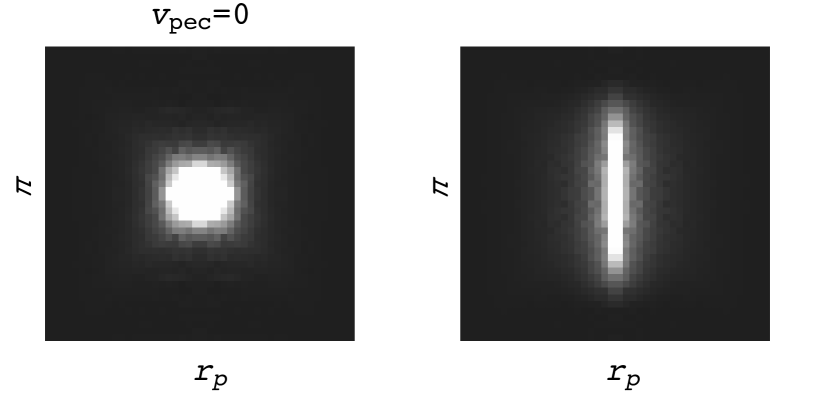
Full information on the object clustering and peculiar velocities is contained in the two-dimensional correlation function, . An example derived from the numerical simulations we use in this Paper is shown in Fig. 1. See, e.g., Zehavi et al. (2002) for an example of the detailed modeling of the function measured for the SDSS galaxies. Unfortunately, such a detailed modeling is impossible for the present high- AGN samples due to limited statistics. However, we show that useful information can still be obtained using projections of on the radial velocity direction and on the sky plane, and , respectively (formally defined in § 3.1 below). Using numerical cosmological simulations, we show that if a substantial fraction of objects lie in satellite galaxies, is expected to be significantly in excess of in the range of comoving distances Mpc (§ 4.3). The observed correlation functions do not show such an excess (§ 5.1), which we exploit to put an upper limit on the fraction of X-ray AGNs in the satellite galaxies. Finally, we explore the redshift evolution of the clustering length and compute the typical mass scale of the AGN host dark matter halos and put constraints on the AGN duty cycle.
All cosmology-dependent quantities are computed assuming a spatially flat model with parameters and (best-fit CDM paramaters obtained from the combination of CMB, supernovae, BAO, and galaxy cluster data, see Vikhlinin et al., 2009). All distances are comoving and given with explicit -scaling, where the Hubble constant is km s-1 Mpc-1. The parameter uncertainties are quoted at a confidence level of 68%.
2. AGN Sample
We use a sample of high- AGNs derived from the Chandra X-ray survey in the 9.3 deg2 Bootes field of the NOAO Deep Wide-Field Survey (Murray et al., 2005). The region was uniformly covered with a grid of overlapping 5 ksec ACIS-I pointings providing a sensitivity of erg s-1 cm-2 in the 0.5–2 keV energy band (Kenter et al., 2005). Extensive optical data exist for this field and 98% of X-ray sources have optical or infrared counterparts (Brand et al., 2006). The redshifts for X-ray sources with optical counterparts brighter than were uniformly obtained with the MMT/Hectospec instrument in the AGN and Galaxy Evolution Survey (AGES, C. S. Kochanek et al., in preparation). Further details on the X-ray and optical observations can be found in Hickox et al. (2009).

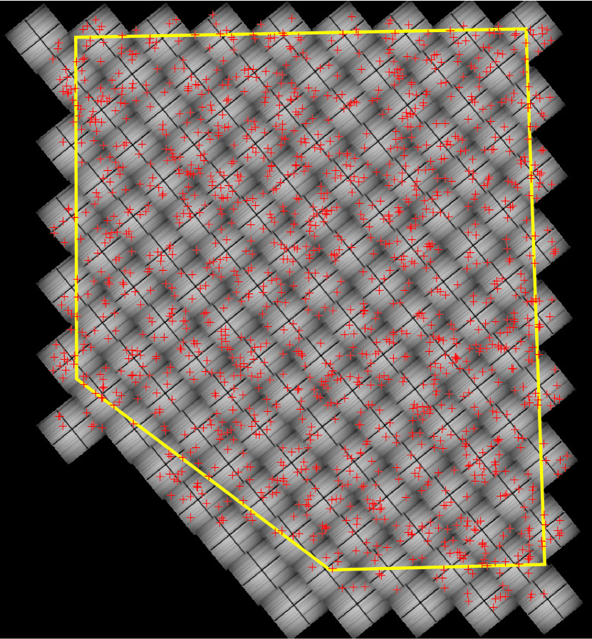
For clustering analysis, we use 1282 X-ray selected AGNs with spectroscopic redshifts. Redshift measurements effectively introduce an additional selection criterion for the sample, based on the optical magnitude of the counterparts, . This selection removes of the X-ray sources and likely introduces a high- cutoff in the redshift distribution of our sources (§ 2.2). Fortunately, the redshift measurements were done with Hectospec (Fabricant et al., 2005) in several passes, which excludes the so called “fiber collisions” problem. The locations of X-ray sources with spectroscopic redshifts are marked in Fig. 2, and their luminosity-redshift diagram is shown in Fig. 3.
To reconstruct the correlation function of sources, we need to simulate catalogs of randomly distributed sources whose distribution follows the sensitivity variations and the redshift distribution of our catalog. Below, we describe how these functions were derived from our Chandra sample.
2.1. Spatial variations of sensitivity
Chandra sensitivity for the detection of point X-ray sources is not uniform across the field of view. Sensitivity variations (, see below) are imprinted on the distribution of detected sources. The typical spatial scale of the sensitivity variations is several arcmin, which corresponds to the comoving distance of Mpc at . This is comparable to the distance scale where we measure clustering, therefore these variations must be taken into account.
The sensitivity variations are caused mainly by two effects — 1) the vignetting of the Chandra X-ray telescopes, and 2) the degradation of the Point Spread Function (PSF) away from the optical axis. The mirror vignetting is well-calibrated and its effect can be computed for a given source population. However, the effects of PSF degradation on the source detection efficiency in the low-photon regime are very complex. Therefore, it is best to measure the combined effect of the sensitivity variations empirically.
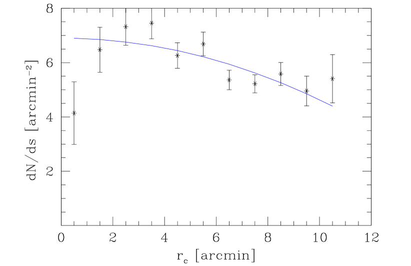
Both the mirror vignetting and PSF degradation are approximately azimuthally symmetric. Therefore, we can assume that the detection sensitivity is a function of the source offaxis angle, and measure it from the radial profile of the surface density distribution of detected X-ray sources, averaged over all the 126 fields. The results are shown in Fig. 4. For a uniform sensitivity, we would expect a constant surface density, while in reality we find that the average surface density is arcmin-2 near the optical axis, and falls to arcmin-2 at off-axis distances of 10 arcmin. The derived radial profile of the source surface density can be modeled with a second-order polynomial,
| (1) |
In addition to this gradual variation with radius, there are sharp features in the spatial sensitivity pattern related to the gaps between the ACIS-I CCDs. In particular, these gaps are responsible for the drop in the number of detected sources at in Fig. 4. These sensitivity variations can be adequately taken into account using the standard Chandra exposure maps. In doing so, we assume that the expected surface density of X-ray sources at a given location is proportional to the effective exposure at this location. This assumption is justified because the source detection in the Chandra/Boötes survey is well in the photon-limited regime (the background is unimportant) and the observed cumulative source counts are very close to around our flux limits (Hasinger et al., 1993; Vikhlinin et al., 1995).
Our final sensitivity map (Fig. 2) consists of the merged set of Chandra exposure maps computed for the individual 126 pointings, each multiplied by the radial sensitivity pattern given by eq. (1). This sensitivity map is taken into account in the derivation of the correlation function through the generation of the appropriate catalogs of random sources. The total area within the conservative boundaries of the spectroscopically surveyed region of the Bootes field is 7.30 deg2. The total effective area, taking into account the gaps between the Chandra CCDs and degradation of the detection efficiency, is 5.90 deg2.
2.2. Redshift distribution
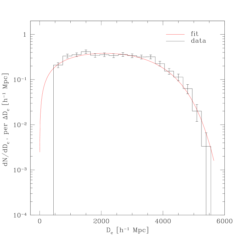
The model for the source redshift distribution, , should reflect both the intrinsic variations of the comoving number density with redshift and all selection effects of the catalog. A commonly used approach is to model the observed distribution with a high-order polynomial (see, e.g., Croom et al., 2005; Ross et al., 2009, for recent examples). This approach works well for catalogs with a large number of sources. However, for smaller catalogs, like ours, there is a danger that a high-order polynomial fit will follow statistical fluctuations in the observed , while a low-order polynomial would be unable to adequately model the strong gradients at low . Therefore, we fit the redshift distribution of AGNs in the Boötes field with a parametric model based on several physical assumptions.
The first component of the model represents the cosmological comoving volume per unit redshift, . The second component is a power law function of the minimum luminosity which corresponds to the Chandra flux limit at redshift , , where is the luminosity distance. This component represents the effect of the low- cutoff of the intrinsic luminosity function introduced by the selection which is primarily based on Chandra detections. It also can describe the evolution of the luminosity function at high . The third component is a high- cutoff modeled by a broad Gaussian, . This component can represent the high- cutoff or steepening of the intrinsic AGN luminosity function, and also can describe various observational limits implicitly built into our catalog (e.g., a lower efficiency of optical identifications and redshift measurements for the highest- X-ray sources). This simple analytic model,
| (2) |
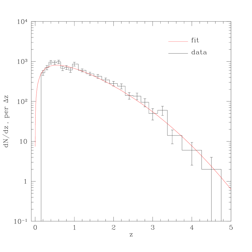
which has only two free parameters provides a strikingly good fit to the observed redshift distribution of the Boötes X-ray selected AGNs (Fig. 5). The best-fit values are and Mpc. We use the arguments outlined above only as a motivation for a good analytical description of the distribution for our sources. The functional form and derived parameters are not meant to represent the true X-ray luminosity function or its evolution.
Figure 5 also demonstrates the general characteristics of our sample. The peak in the observed distribution is near . The median redshift of the sample is . The tail in the redshift distribution extends to but the fraction of AGNs with is very small. Overall, the clustering properties of sources in our sample are most sensitive to the distribution of the X-ray AGN population near .
3. Two-point Correlation Function of Chandra/Boötes AGNs
3.1. Definitions
Because the volume is never sampled completely in astronomical surveys, the derivation of the two-point correlation function from the data uses mock catalogs of intrinsically randomly distributed objects, which faithfully reproduces all observational distortions introduced by the survey. Examples of such distortions are boundaries of the survey region, gaps in the data or spatial variations of the sensitivity, variations of the selection efficiency with redshift, etc. Given the catalog of observed sources and the mock random catalog, the two-point correlation function can be estimated (Landy & Szalay, 1993) as
| (3) |
where is the number of source pairs in the data for the given distance interval, is the corresponding number of pairs in the random catalog, is the number of pairs between the data and random catalog, and and are the numbers of objects in the data and random catalogs, respectively. Statistical uncertainties for can be estimated as
| (4) |
(Peebles, 1973); this equation includes both the Poissonian shot noise and intrinsic variance terms. To verify the accuracy of the error by eq. 4, we used the sample varience of the correlation functions measured in the mock catalogs derived from the Millenium simulation (Kitzbichler & White, 2007) for the survey geometry and object properties similar to those of the Chandra/Boötes survey. This analysis showed that eq. 4 is accurate at tsmall scales but may underestimate the uncertainties at large scales. The correction factor can be described by a smooth function which is 3%, 23%, and 42% at separations of , , and Mpc, respectively. This correction is applied to the statistical uncertainties estimated by eq. 4.
The correlation function in real space is expected to be isotropic, so is a function of the 3D separation only. When the object redshifts are used to derive the distances, the correlation function is distorted in the line-of-sight direction because of large-scale flows (the Kaiser 1987 effect) and “fingers of God” arising within the virialized dark matter halos. The correlation function should then be measured as a function of the projected separation, , and the line-of-sight separation, . Equations [3] and [4] still can be used, but the pairs must be counted for each combination .
Given the angular separation between two objects, , and redshifts, and , the comoving separations and can be computed as follows. First, one computes the radial comoving distances, and , corresponding to the object redshifts (see, e.g., Hogg, 1999). Then, following Davis & Peebles (1983) we have
| (5) |
| (6) |
One can also define a formal 3D separation,
| (7) |
but it should be kept in mind that is not equivalent to the true 3D separation, , because of the redshift space distortions.
As only the line-of-sight separations, , are affected by the object peculiar velocities, it is useful to consider the correlation function projected on the sky plane,
| (8) |
because it is not modified by the redshift-space distortions (Davis & Peebles, 1983):
| (9) |
Because of the insensitivity of to the redshift-space distortions, most of the studies which involve detailed modeling of the shape of the galaxy two-point correlation function are based on fitting the measurements (e.g., Zehavi et al., 2005; Padmanabhan et al., 2009). Using instead of is particularly straightforward in those cases when can be sufficiently accurately approximated by a power law, . It follows from eq. [8] that in this case the relation between and is simply (Peebles, 1980)
| (10) |
where
| (11) |
Therefore, the correlation length, , and the slope of the true 3D correlation function can be obtained immediately from the power-law fit to .
Below, we also use a projection of the measured 3D correlation function on the line-of-sight direction,
| (12) |
In the absence of peculiar motions, should be equivalent to . In particular, for a power-law , eq. [10] will be valid also for .
Large separations do not contribute significantly to the integrals in equations 8 and 9 but add noise, therefore in practice the integration is truncated at some finite separation. A good choice for studies of AGN samples is to truncate the integration at Mpc (see, e.g., Gilli et al., 2009). Following this and other works we investigated how the derived correlation length depends on the choice of the cutoff distance (see, e.g., Fig. 9 in Gilli et al. 2005 or Fig.3 in Allevato et al. 2011). For our sample, the convergence is reached at a cutoff radius of Mpc (for cutoffs between 20 and Mpc, the derived varies by less than 4%). Based on this analysis, we trancated the integration at comoving separations Mpc, and further reduced the sensitivity of our results to this choice by applying small corrections to the integrated functions. Assuming that the true correlation function follows a power law with index at large separations, we can calculate the effect of this truncation as
| (13) |
The correction coefficient, , is close to 1 for Mpc and gradually decreases at larger distances. For (close to our best-fit value), at Mpc, 0.87 at Mpc ( the correlation length), and 0.63 at Mpc ( the largest separation at which the projected correlation is still marginally detectable).
Using equations 10 and 13, we can define the quantities
| (14) |
| (15) |
where is determined from the power-law fit to the measured (eq. [10]). Thus defined, should be a close approximation to the true 3D correlation function . In the absence of redshift-space distortions, also should approximate . However, the peculiar motions (and in particular, the “finger of God” effect) suppress on the smallest separations and enhance it relative to on intermediate scales (see below). Therefore, can be used to determine the correlation length of our objects and hence the mass scale of their host dark matter halos. The ratio reflects the amplitude of the peculiar motions and hence can be used to constrain the fraction of objects located in the satellite dark matter subhalos.
3.2. Results
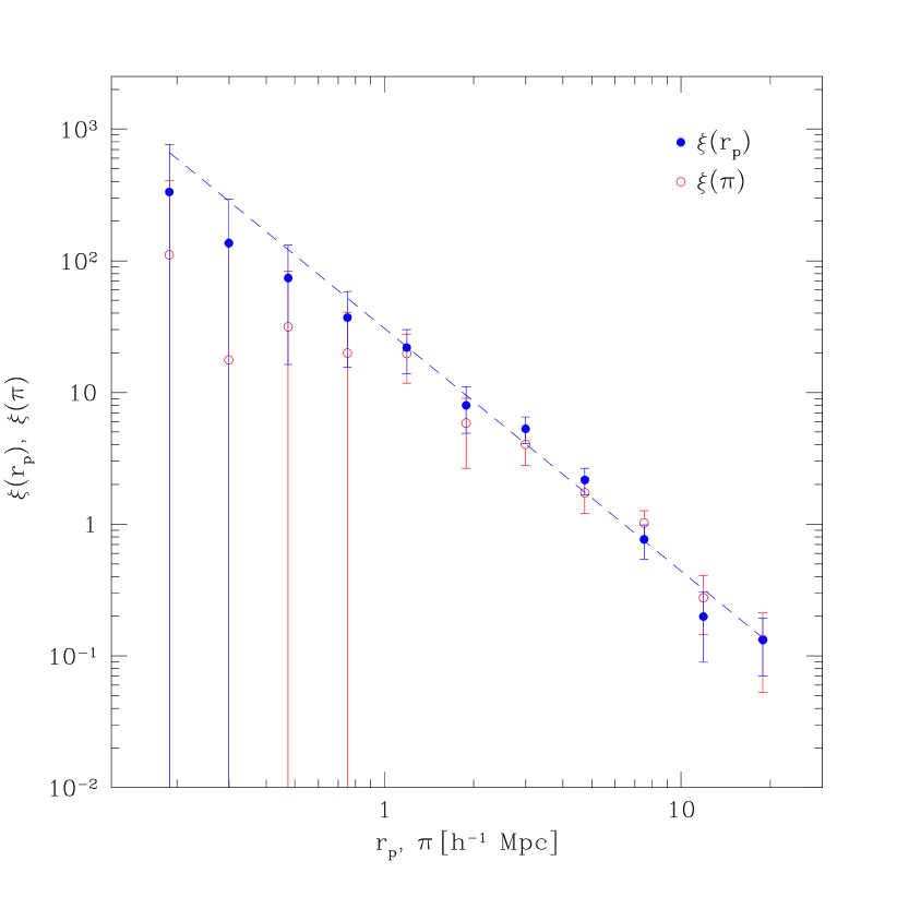
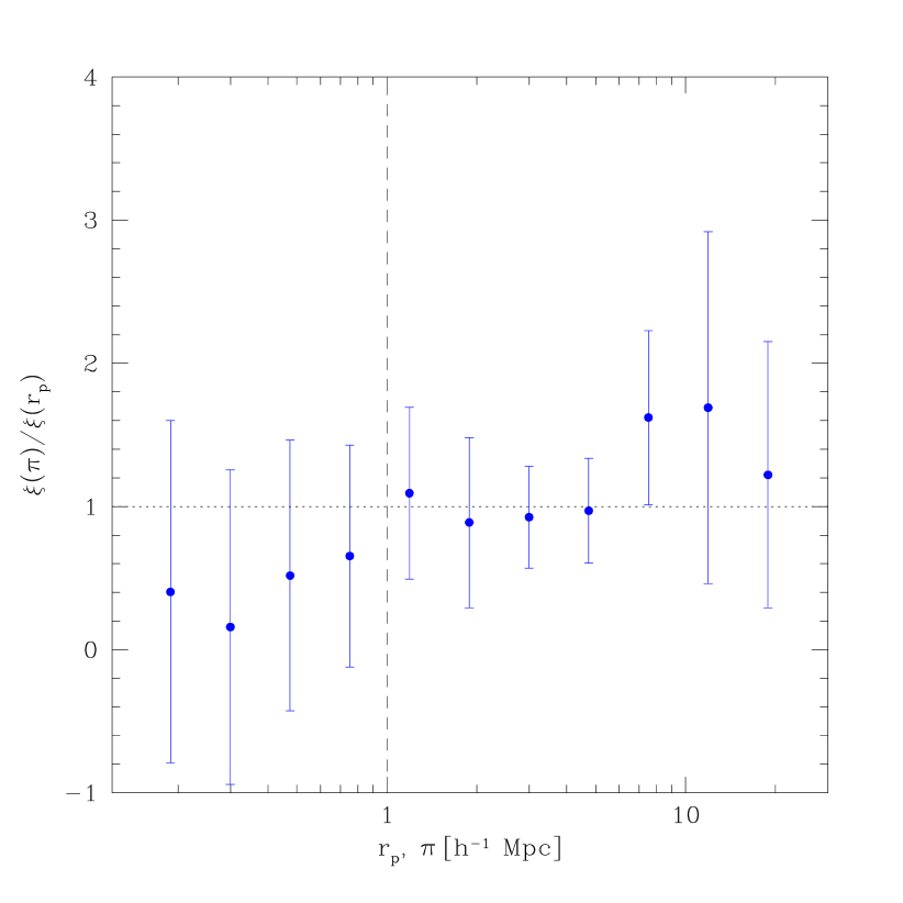
The correlation functions and derived for our complete sample are shown in Fig. 6a (filled and open circles, respectively). Technically, we derive the functions as follows. First, we estimate the two-dimensional correlation function, , on a grid of separations with equal logarithmic width for each cell, . We use the Landy & Szalay estimator (eq. 3). The random catalog is generated using the spatial sensitivity map and the model for the redshift distribution in our sample (§ 2.1 and 2.2). To minimize the additional noise, the number of objects in the random catalog is a factor of 100 larger than that for the AGN sample. The derived is then integrated in the radial and sky plane directions to obtain and (eq. 9 and 12). As discussed in § 3.1, the integration is limited to separations Mpc to minimize noise. We then fit a power law (eq. 10) to to measure the slope of the correlation function, . The correlation length measured for the full sample is Mpc. We then compute the renormalization factor (eq. 11) and correct for the truncation of the integration in and at Mpc (eq. 13). With the renormalization factors determined, we convert and into and using eq. [14–15].
As discussed above, should be close to the true 3D correlation function , while should be distorted by peculiar motions of the AGN host galaxies. Indeed, we observe a suppression in relative to at separations Mpc. Unfortunately, the corresponding radial velocity difference, , is uncomfortably close to the uncertainties in the AGES redshift measurements (Kochanek et al., in preparation). Therefore, we ignore the data at Mpc. At intermediate separations (Mpc), is expected to be enhanced by the peculiar motions (see below). No such enhancement is present in the data. In fact, the ratio is fully consistent with 1 at separations Mpc within the measurement uncertainties222The uncertainties of the ratio are computed by propagation of uncertainties in and . In principle, a region in the 2-dimentional enters into both projections. However, the analysis shows that the data in this region contribute negligibly to the “signal” and “noise” in the ratio, so our simple uncertainty calculation is adequate. (Fig. 6b). Below, we show that this can be used to put an upper limit on the fraction of AGNs that can reside in satellite galaxies orbiting within massive dark matter halos.
3.2.1 Comparison with previous measurements
Our results represent the most accurate measurement of the spatial clustering of X-ray selected AGNs to date, so a comparison with earlier observations is useful.
The first detection of angular clustering of X-ray sources was reported by Vikhlinin & Forman (1995) based on the analysis of the ROSAT PSPC data. Using the Limber equation reconstruction (Peebles, 1980), these authors estimated a correlation length of Mpc (comoving) at using raw measurements, and Mpc after correcting for the “amplification” bias caused by the poor angular resolution of the ROSAT PSPC. The latter value is in good agreement with our results.
Our results also are in good agreement with direct measurements of the spatial clustering in the ROSAT NEP survey (Cappelluti et al., 2007), Chandra surveys in Deep Fields North and South (Gilli et al., 2005), and the XMM-Newton COSMOS field (Gilli et al., 2009). The correlation length we measure in the low redshift bins (see §5.2 below) is in good agreement with Mpc found in two studies based on cross-correlations of X-ray AGNs with galaxy catalogs Hickox et al. (2009); Coil et al. (2009), although is higher than the Mpc reported in a similar work by Krumpe et al. (2010).
Correlation lengths for the X-ray AGNs have been estimated also from the Limber inversions of the angular clustering measured for the XMM-Newton and Chandra sources. A wide range of values can be found in the literature (e.g., Plionis et al., 2008, and references therein); our measurements are inconsistent with Mpc reported in some of these analyses.
4. AGN Clustering Model
In the past ten years, a very successful framework for modeling the nonlinear clustering properties of galaxies has been developed (the so called Halo Occupation Distribution (HOD) model, see Seljak, 2000; Ma & Fry, 2000; Peacock & Smith, 2000; White et al., 2001; Scoccimarro et al., 2001; Berlind & Weinberg, 2002; Berlind et al., 2003, among others). The approach is based on the idea that the distribution of dark matter can be fully described through the mass function, linear bias, and density profiles of dark matter halos. These elements are well-calibrated using -body simulations. The two additional ingredients of the model, which are less well known, are the probability distribution for a halo of mass to contain galaxies, and the distribution of galaxies within the halos. These functions can be parameterized by the functions suggested by the results of high-resolution numerical simulations (e.g., Kravtsov et al., 2004), and some parameters of the model can be in fact determined by fitting the observed correlation functions. In particular, Kravtsov et al. (2004) and Zheng et al. (2005) show that the elements of HOD can be effectively decomposed into two components, separately describing the properties of central and satellite galaxies within the dark matter halos.
The HOD model is now very well developed for fitting the shape of the two-point correlation function. This technique has been applied to modeling the projected two-point correlation functions, , for objects ranging from Lyman-break galaxies at (Conroy et al., 2006) to relatively low- quasars from SDSS (Padmanabhan et al., 2009). Recently, the HOD approach has been developed also for modeling the redshift-space distortions in the galaxy correlation functions (Tinker et al., 2006; Tinker, 2007) — just the type of information we are aiming to use in this work to constrain the locations of Bootes/Chandra AGNs within the host dark matter halos.
In principle, the HOD models for galaxy clustering are analytic, and thus are convenient for those applications in which the cosmological parameters are varied. However, some of the most essential parameters of the HOD models are calibrated using numerical simulations. If one is interested in varying the parameters of galaxy distribution at a fixed redshift in a fixed cosmological model, it is more accurate — and easier — to obtain the model correlation functions directly from numerical simulations rather than to rely on analytic approximations derived from analyzing the simulations. This is the approach we take here.
4.1. Numerical Simulations
The set of simulations we use in this work is described in Tasitsiomi et al. (2004) and Conroy et al. (2006). These are high-resolution dissipationless simulations run in a flat CDM cosmology with parameters close to the present-day “concordance” values, , , and . The simulations follow the evolution of dark matter in a Mpc box. The box contained dark matter particles with mass ; the peak resolution reached kpc.
The locations and velocities of the dark matter particles in the simulations were recorded at , 0.5, 1.0, 2.0, 3.1, 4.0, and 5.0, matching well the redshift distribution in the Bootes/Chandra AGN sample (see Fig.5). The simulation outputs were then analyzed to identify dark matter halos and subhalos using a modification of the Klypin et al. (1999) bound density maxima halo-finding algorithm (see Kravtsov et al., 2004, for details). The main steps of this procedure are identification of local density peaks, and analysis of the density, circular velocity, and velocity dispersion profiles with simultaneous removal of unbound particles. The final profiles, using only bound particles, are used to calculate the halo properties such as the circular velocity profile and the maximum circular velocity, . The completeness limit for halo identification using this procedure is particles. The corresponding limit is km s-1, and the associated mass limit is . The best-fit power law to the relation333Hereafter, we use the mass defined within an overdensity threshold of 180 with respect to the mean density of the Universe at the given redshift. The correspondence between and mass is quoted for unless the redshift is stated explicitly. derived in these simulations at is
| (16) |
where the velocities are in units of km s-1 and masses are in units of .
The identified halos were then classified into host halos whose centers are not located within any larger virialized systems, and subhalos which lie within the virial radius of a larger system (see Tasitsiomi et al., 2004, for details of this procedure). Briefly, a halo is classified as a subhalo if its center is within of the center of a more massive halo, where is the radius which corresponds to a mean spherical overdensity of 180 relative to the mean density at the given redshift. In the real Universe, centers of host halos can be identified as locations of the groups’ central galaxies, while subhalos correspond to satellite galaxies.
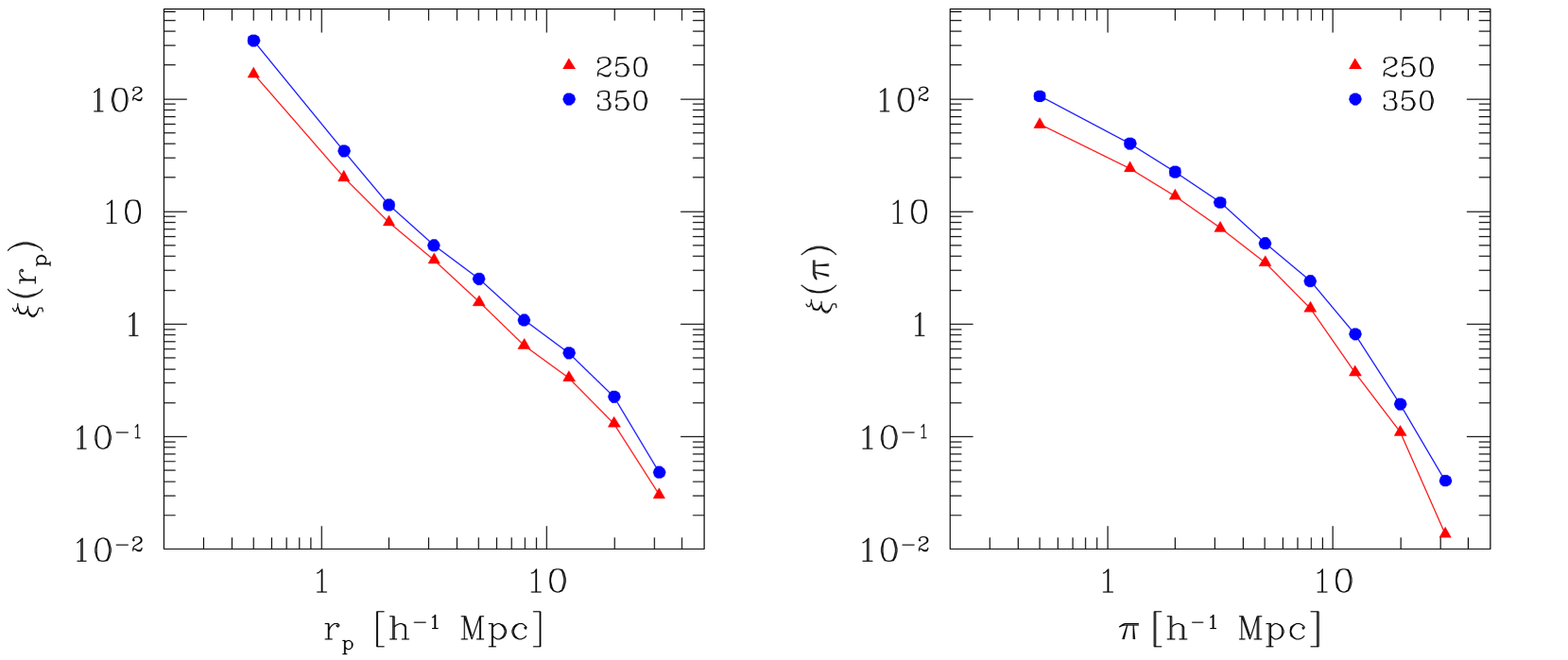
4.2. Model of the AGN population
Our data can constrain the following two basic properties of the AGN population. First, the overall clustering amplitude observed in constrains the mass scale of the AGN host dark matter halos. Note that it is the mass scale of host halos, not of individual subhalos in which the AGNs might reside, which is constrained by the amplitude. For example, a population of small subhalos with km s-1 which are located within larger halos with km s-1 has the clustering length which closely matches that for larger, parent host halos, and not that for the entire population of km s-1 halos. Therefore, the first parameter of the model we use to characterize the spatial distribution of AGNs is the minimum for the halos which can contain the X-ray AGNs. The AGN can be located either at the center of such a halo or in any of its smaller subhalos.
Note that we choose to characterize the halos using their rather than the virial mass for the reasons outlined in Kravtsov & Klypin (1999), Nagai & Kravtsov (2005), and Conroy et al. (2006). The maximum circular velocity is a more direct measure of the depth of the halo potential wells. It reflects the central properties of the halo better, and is less subject to the effects of tidal stripping, than the halo virial mass which is dominated by the matter at large radii. Therefore, we can expect that the stellar content of the halo and all baryonic processes in the center, including the AGN activity, are better correlated with than with . Nagai & Kravtsov (2005) and Conroy et al. (2006) argue further that the best indicator for the stellar mass of subhalos is their before accretion onto the host halo. Since our results are not very sensitive to the threshold for subhalos (see below), we do not make this distinction.
For a fixed threshold of the host halo , the correlation length of astronomical objects only weakly depends on whether these objects are located in the halo central galaxies or in smaller subhalos. As discussed above, the ratio should be a much more sensitive and direct indicator for the satellite fraction. We parameterize this fraction by the probability, , for objects to reside in the central galaxies of host halos; is, therefore, the probability for objects to reside in any of the smaller subhalos. The two parameters, the threshold, , and the probability , fully specify the relation between our model AGN population and the dark matter halos and subhalos identified in the numerical simulations. is primarily constrained by the correlation length of , and is mostly constrained by the ratio444Note that we assume that is independent of and we have not explored the models in which is very different for the most massive halos. Effectively, our derived constraints correspond to a mean in the velocity range , containing of halos with (Klypin et al., 2010)..
Algorithmically, we simulate the AGN locations by randomly drawing the halos and subhalos from the simulation box according to the parameters and . First, we select all bound structures (both halos and subhalos) with km s-1. This threshold is slightly higher than the resolution limit in the simulations. We verified that the final results are nearly the same when this initial threshold is varied between 50 km s-1 and 100 km s-1. We then select only those subhalos which are contained within halos with above the given value of . We then randomly put a small number of objects (10–100) within the simulation box555This is done to approximate the low space density of Chandra/Boötes AGNS.. With the probability , the object is associated with one of the selected subhalos, and with the probability it is put in the center of one of the halos. This procedure is repeated multiple times randomly selecting one of the box axes as the line of sight. Using these simulated objects, we derive a model of and for each combination of and .
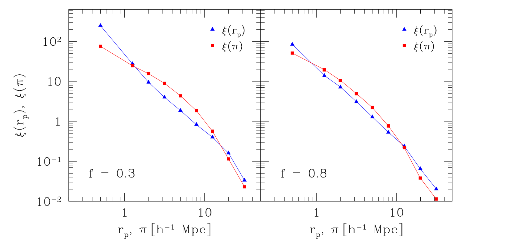
4.3. Model Correlation Functions and
The correlation functions and were derived from the simulation outputs on a grid of parameters within the range km s-1 and . Examples are shown in Fig. 7 and 8. Comparison of the two panels in Fig. 7 illustrates the effect of on the correlation functions. For smaller (more objects located in satellite galaxies, left panel), the projected correlation function shows a stronger component at Mpc in excess of a power law extrapolation from larger separations. This excess is attributed to the “1-halo” term in the analytic halo model of the correlation function. At the same time, shows a larger suppression of the correlation amplitude at Mpc with respect to at the same separations, and a stronger enhancement over at Mpc for small . This is the consequence of a stronger “finger of God” effect in the case when more objects are located in the satellite galaxies. Unfortunately, the statistical uncertainties in the real data do not allow a detailed modeling of the observed at small separations. Modeling of the at small separations is further complicated by the effect of uncertainties in the redshift measurements (§ 3.2). At large separations, of the simulation box size, the correlation functions derived from the simulations are not reliable (Kravtsov et al., 2004; Colín et al., 2006; Conroy et al., 2006). Taking all these considerations into account, we will match the observed and model correlation functions in the intermediate range of radii, Mpc.
First, we compute the correlation length, , for each combination . This is done by fitting a power law function, , to in the range Mpc. We then compute the ratio (an example is shown in Fig. 9) and fit it in the same range of separations with a modified log-normal function,
| (17) |
The index is fixed at the mean best-fit value for all combinations, . The ratio derived from the simulations shows substantial variations related to cosmic variance (this can be estimated by comparing the results for three viewing angles, see errorbars in Fig. 9). Therefore, we need to smooth the results of the fit by eq. 17. This is achieved by fitting low-order polynomials to the parameters , , and as a function of and . We found that an adequate description is achieved if the best-fit values of and are approximated as a linear function of , and is fit by a second-order polynomial. An example of the fitting function derived from this smooth map is shown in Fig. 9. Due to the size of the simulation box, the uncertainties in the smoothed model are still finite, but we verified that they are negligible compared to those in the data.
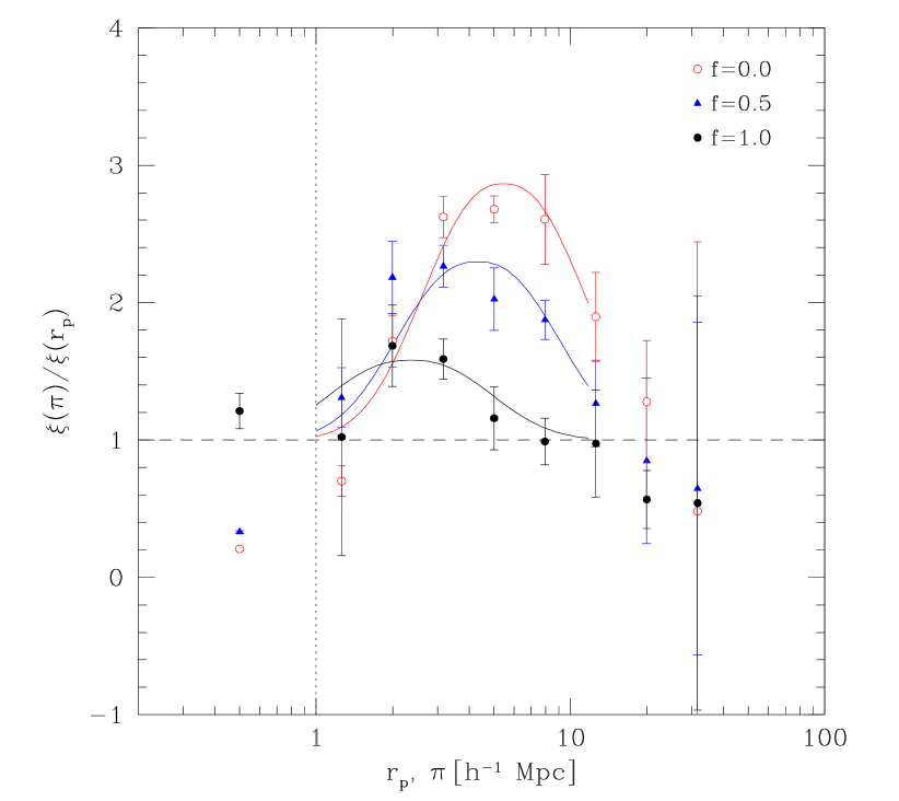
4.4. Application to the Data
In applying the correlation function model to the data we avoid including any sensitivity to the slope of the correlation function. The primary motivation is that our method assigning the AGN locations to the dark matter halos may be overly simplistic to correctly predict the details of the correlation function shape. Also, the cosmological parameters used in the simulation are slightly different from the currently accepted values, resulting in a systematic difference in the shape of the perturbation power spectrum in the simulated and real universes. This said, the models derived from simulations do provide a good fit to the data (see discussion in § 5.1 below).
Based on these considerations, our includes two components. First, we use the value of the correlation length derived from fitting the function (§ 3.2). Second, we use the ratio in the range of separations Mpc (the data at Mpc are not used because they are likely affected by the redshift measurement uncertainties, see §3.2). For halos with circular velocities km s-1 (as indicated by the amplitude of the AGN correlation function, see below), the “fingers of God” extend to Mpc, just in the middle of this range of separations. Formally, the constraints on the parameters of the AGN population model, and , are derived using a function computed as
| (18) |
where the summation in the second term is over the data points in the Mpc separation range, and the model functions are those described in § 4.3.
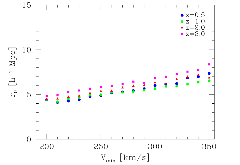
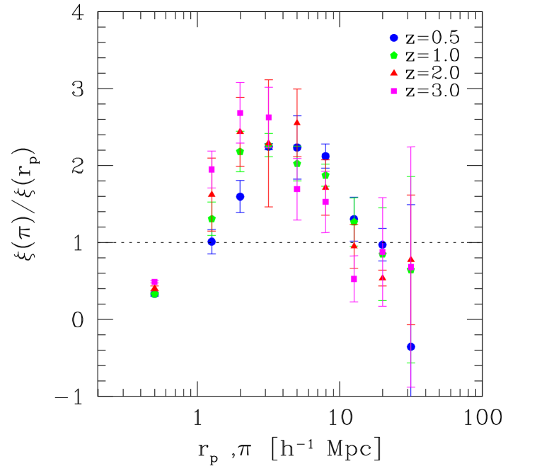
4.4.1 Redshift Trends
The procedure described above provides a correlation function model at the redshifts where the simulation outputs were saved. The Chandra/Boötes AGNs span a wide redshift range and we have to bin the data into several redshift intervals to achieve an acceptable level of accuracy for the correlation function measurements. Therefore, we need to account for any -dependent trends of the correlation function models.
Fortunately, for our choice of observables, and the ratio, the redshift trends are very weak. This is illustrated in Fig. 10. The left panel shows as a function of for a population model with (all objects are at the centers of distinct halos) for the simulation outputs at , 1, 2, and 3. Obviously, there is almost no change in for a fixed at . Any changes are much smaller than the uncertainties of our measurement even for the full sample. Therefore, we conclude that the model as a function of does not evolve over our redshift range of interest.666Note that as a function of mass does evolve with redshift, as expected. However, this evolution appears to be canceled by the evolution in the relation and the trend of with at a given redshift. The ratio also shows little, if any, evolution with redshift. The right panel in Fig. 10 shows the results for the population model with km s-1 and (50% of objects are in the satellite subhalos of km s-1 halos). Any difference between the simulation outputs is within the uncertainties (estimated from analyzing three different projections for each simulation output).
The lack of evolution in the clustering model over our redshift interval (and also the lack of detectable evolution of with , see § 5.2 below) indicates that we can safely combine the data over the entire redshift range in the sample. Furthermore, there is no need to weight the models with the redshift distribution — one simply can use the results for the simulation output at . We take this approach in fitting the parameters of the population model, and (§ 5.1). In addition, we constrain the evolution of with (§ 5.2) under the assumption that the fraction of AGNs in the subhalos does not evolve (i.e., using a fixed derived from the analysis of the entire sample).
4.4.2 Adjusting the Results to a Low- Cosmology
Finally, we note that the numerical simulations we use were run assuming a high value of the power spectrum normalization, at . This results in an incorrect prediction of the correlation amplitude for halos of a given mass, and thus slightly biases the derived parameters of the AGN population model, in particular, . Obviously, it would be best to use the simulations performed for the currently favored cosmological model with but in general, these were unavailable at the time of this investigation. In Appendix A, we describe a procedure which can be used to scale the results from the comparison with the simulation to any desired cosmology. In particular, if we use the best-fit flat CDM cosmological model derived from the joint analysis of the galaxy cluster mass function and other cosmological datasets, and (Vikhlinin et al., 2009), the masses reported below should be scaled by a factor of , the ’s decreased by 10%, and the number density of objects increased by 20%.
5. Modeling Results
5.1. and the Satellite Fraction for the Entire Sample

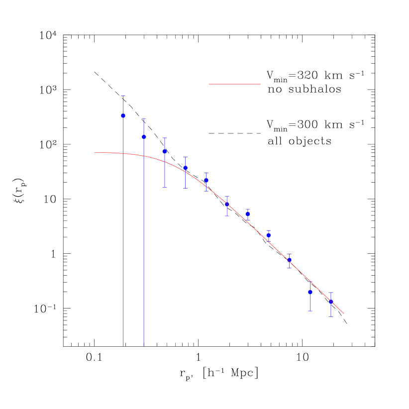
.
Figure 11 shows the combined constraints on the population model parameters, and , obtained from fitting the full sample of Chandra/Boötes AGNs. The best-fit velocity threshold is km s-1 (68% CL one-parameter uncertainty). At , this corresponds to , or after correcting for the lower- cosmology (see § 4.4.2 and Appendix A)777Hickox et al. (2009) quote a higher mass, for an X-ray AGNs sample with the mean , from which they measure Mpc. The main source of the difference, as explained in Conroy et al. (2008, see their p.1195), is a more accurate model for the matter power spectrum at galactic scales deployed in modern simulations such as those we use here.. We thus conclude, in agreement with the earlier studies (Gilli et al., 2009; Hickox et al., 2009), that the X-ray AGNs at high redshifts reside in small galaxy groups with masses of a factor of a few above the present-day mass of the Milky Way.
As expected from the striking agreement of the observed and projected correlation function, the best fit is , i.e. all AGNs are located at the centers of distinct dark matter halos. The 90% CL upper limit on the satellite fraction is . This is significantly lower than the fraction of suitable subhalos in the simulation box. For example, within the 1486 halos with km s-1 there are 683 Milky Way-type subhalos (km s-1), and many more smaller galaxies. If all these galaxies had a uniform probablity to host an X-ray AGN, we would expect .
If we consider only the objects with km s-1, 11% of them are satellites in more massive halos, which is comparable to the upper limit for derived from our model. However, we still can exclude a uniform probability for hosting an AGN in this case, because the km s-1 subhalos by definition are members of more massive halos, and thus have higher peculiar velocities than most of the satellites in our model. To illustrate this point, we computed the project correlation functions for all halos and subhalos with km s-1 (Fig. 12). This population has nearly the same correlation length as our best-fit model with . In the function there is a strong “1-halo” component at Mpc. We do not observe such a component in the AGN autocorrelation function, even though the quality of data at small scales is clearly insufficient for distinguishing the models. However, the km s-1 dark matter subhalos are mainly satellites in much more massive halos (median for their host halo is 530 km s-1). They have high peculiar velocities and show a strong excess in over at separations Mpc, not present in the data.
Therefore, we can conclude that the X-ray AGNs at tend to avoid massive galaxies in the outskirts of yet more massive groups and clusters, or satellite galaxies in the km s-1 galaxy groups. Instead, the AGNs are preferentially located at the centers of distinct dark matter halos.
5.1.1 Comparison with Previous AGN HOD Studies
Our conclusion on the preferential location of AGNs in the halo central galaxies contradicts the results of Padmanabhan et al. (2009, P09 hereafter) who observe the presence of the 1-halo term in the cross-correlation function of optically-selected quasars and Luminous Red Galaxies (LRGs), and use this to conclude that a large fraction of the AGNs is hosted by satellite galaxies.
There are obvious differences in the AGN populations studied in P09 and our work. A striking mismatch in the derived host halo masses — estimated in P09 is a factor of lower than our minimum mass — indicates that we indeed may be dealing with different object populations. However, we also note a significant difference in the underlying methods. While our results follow from the AGN auto-correlation function, the P09 approach is based on cross-correlation of the AGNs with LRGs, the tracers typically located in the halos a factor of more massive than the AGN hosts (see, e.g., Table A1 in P09).
Recently, Miyaji et al. (2011, M11 hereafter) published the halo occupation analysis for a sample of X-ray selected AGNs. Their AGN sample is at lower redshifts () but closely matches ours in terms of the estimated host halo mass. Similarly to P09, M11 detect a 1-halo term in the cross-correlation function of AGNs and LRGs, qualitatively indicating that some fraction of the AGNs may be located in the satellite galaxies. However, even if the 1-halo term is detected, the best-fit AGN HOD models of M11 imply that the AGN incidence rate in the satellite galaxies decreases with increasing halo mass, approximately in line with our conclusions above.
In summary, we can only speculate whether any differences in our conclusions with those of P09 and M11 are due to not identical AGN samples (optical vs. X-ray selection, or a substantial mismatch in the typical X-ray luminosities in the M11 and our samples), or different analysis methods (velocity space auto-correlation function of AGNs vs. their spatial cross-correlation with more massive tracers). A clear answer can be provided by detection of, or strong upper limits on, the 1-halo term in AGN auto-correlation function. Unfortunately, the present data quality is insufficient for this purpose.
| Redshift range | ||||||||
|---|---|---|---|---|---|---|---|---|
| (2) | (3) | (4) | (5) | (6) | (7) | (8) | (9) | |
| 0.374 | 42.58 | |||||||
| 0.738 | 43.34 | |||||||
| 1.279 | 43.85 |
Note. — Column (3) — mean X-ray luminosity in the 0.5–2 keV band (rest-frame). Column (4) — best-fit correlation length assuming a fixed slope of , in units of comoving Mpc. Column (5) — threshold maximum circular velocity of the host dark matter halos, in units of km s-1 (§5.2). Column (6) — the halo virial mass corresponding to , in units of . Column (7) — comoving number density of X-ray sources at , in units of Mpc-3. Column (8) — comoving number density of dark matter halos with at , in units of Mpc-3. Column (9) — probability for the Chandra/Boötes AGNs to be in active state computed as the ratio of number density of AGNs and the dark matter halos with .
5.2. as a Function of Redshift
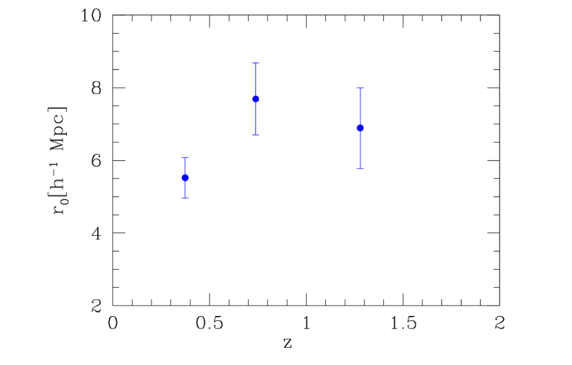
Splitting our Chandra/Boötes AGN sample into 4 subsamples, objects in each, we can measure the correlation length, , as a function of redshift if we hold the slope of the correlation function fixed at the best-fit value obtained for the entire sample, . The in the highest redshift bin, , is poorly constrained, while in the other three samples we obtain reasonably accurate values, given in Table 1 and shown in Fig. 13. There is almost no change in over the redshift interval , with all the measurements being consistent with the average Mpc derived for the entire sample.
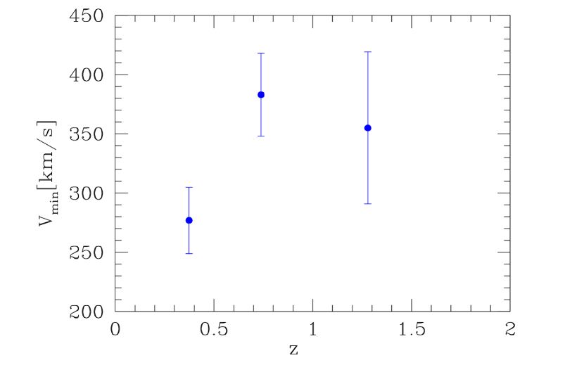
Assuming further a fixed at each , as indicated by modeling of the redshift-space distortions in the entire sample, we can convert the best-fit values of at each redshift to the threshold circular velocity for the parent dark matter halos. The results are shown in Fig. 14. We find no detectable trend of or the corresponding mass threshold, (see Table 1), with redshift, either. This appears somewhat counterintuitive because in a flux-limited sample, such as ours, the objects at higher redshift have higher intrinsic luminosities, and we might expect them to be located in more massive dark matter halos. We note, however, that the studies of optically selected QSOs also indicate a weak or no trend of clustering length with the object luminosity (Croom et al., 2005; Shen et al., 2009). Clustering analysis of the SDSS quasars (Ross et al., 2009) shows mild or no evolution of the real-space correlation length at .
5.3. Constraints on AGN Duty Cycle
Having estimated the mass scale and therefore the space density of Chandra/Boötes AGNs, we can formally compute their duty cycle following the approach of Martini & Weinberg (2001). Under the simplifying assumption that the halo lifetime is approximately independent of mass, the probability for the AGN to be active is simply
| (19) |
where is obtained from the fit (eq. 2) for the median redshift for the given subsample. The limiting X-ray luminosity is ill-defined for our sample because the X-ray detections extend to very low limits in terms of the number of detected X-ray photons (, see Kenter et al., 2005), and in this regime, a wide range of possible intrinsic intensities corresponds to the given number of photons (Kenter & Murray, 2003). However, as a guide for the typical luminosity scale one can use the median reported in Table 1. With these caveats, the probabilities given by eq. 19 and reported in column (9) of Table 1 correspond to the probability for the dark matter halos with to host an AGN with the instantaneous soft-band X-ray luminosity of order or above. These generally decline with mean luminosity and/or redshift. Interestingly, our results indicate that AGNs are quite common at low redshifts — approximately of dark matter halos with km s-1 (or mass ) host an AGN with a soft-band X-ray luminosity of erg s-1 or above.
6. Discussion and conclusions
We measured the clustering properties of X-ray selected AGNs using a sample of 1282 sources with spectroscopic redshifts from the 9.3 deg2 Chandra survey in the Boötes region — one of the most accurate such measurement to date. In agreement with previous studies of X-ray and optically selected AGNs, we find that the real-space correlation function can be approximated in the radial range comoving Mpc by a power law with a slope of . The correlation length is Mpc, showing only weak trends with redshift at (or with X-ray luminosity).
Matching the observed clustering properties of the Chandra/Boötes AGNs to those of dark matter halos in the high-resolution cosmological simulations, we find that the X-ray AGNs reside in halos with the maximum rotational velocity km s-1, or with total masses , also with no detectable redshift trend. The lack of a redshift or luminosity dependence of the AGN clustering is inconsistent with the scenarios in which the AGN luminosities in the active state are similar fractions of the Eddington luminosity. However, it can be explained in the scenario in which the AGN activity is triggered by major mergers of gas-rich galaxies, and the instantaneous luminosity passes through many levels after each trigger (Hopkins et al., 2006).
Our results reveal another interesting aspect of the AGN clustering which was predicted in Hopkins et al. (2008). The redshift measurements in our sample are sufficiently accurate to detect peculiar motions of objects in excess of km s-1. The comparison of the two-point correlation functions projected on the line of sight and on the sky plane reveals no signatures of the redshift-space distortions, which allows us to put limits on the fraction of AGNs located in the satellite subhalos within the host dark matter halos. We find that the X-ray AGNs are predominantly located in the central galaxies of the host dark matter halos and tend to avoid satellite galaxies. Quantitatively, we limit the fraction of AGNs in non-central galaxies to be at the 90% CL. We also exclude the model in which the probability for a galaxy with km s-1 to host an AGN is the same for central galaxies and satellite galaxies in more massive halos (§ 5.1). The central locations of the quasar host galaxies are expected in the trigger model because mergers of equally-sized galaxies preferentially occur at the centers of dark matter halos (Hopkins et al., 2008).
Finally, we compared the number densities of the Chandra/Boötes AGNs to that of the dark matter halos with the mass corresponding to the AGN clustering amplitude. We find that the fraction of halos with active X-ray AGNs decreases with increasing — and, correspondingly, with — probably reflecting a lower probability for an object to have a higher instantaneous luminosity. At the lowest redshifts in our sample, Chandra probes such low luminosity that X-ray AGNs become quite common. At , the Chandra-detected sources are located in more than 10% of the dark matter halos with km s-1 or .
References
- Allevato et al. (2011) Allevato, V., et al. 2011, arXiv:1105.0520
- Angulo & White (2010) Angulo, R. E. & White, S. D. M. 2010, MNRAS, 405, 143
- Bardeen et al. (1986) Bardeen, J. M., Bond, J. R., Kaiser, N., & Szalay, A. S. 1986, ApJ, 304, 15
- Berlind & Weinberg (2002) Berlind, A. A. & Weinberg, D. H. 2002, ApJ, 575, 587
- Berlind et al. (2003) Berlind, A. A., et al. 2003, ApJ, 593, 1
- Bond & Efstathiou (1984) Bond, J. R. & Efstathiou, G. 1984, ApJ, 285, L45
- Brand et al. (2006) Brand, K., et al. 2006, ApJ, 641, 140
- Cappelluti et al. (2010) Cappelluti, N., Ajello, M., Burlon, D., Krumpe, M., Miyaji, T., Bonoli, S., & Greiner, J. 2010, ApJ, 716, L209
- Cappelluti et al. (2007) Cappelluti, N., Böhringer, H., Schuecker, P., Pierpaoli, E., Mullis, C. R., Gioia, I. M., & Henry, J. P. 2007, A&A, 465, 35
- Cappi et al. (2001) Cappi, M., et al. 2001, ApJ, 548, 624
- Coil et al. (2009) Coil, A. L., et al. 2009, ApJ, 701, 1484
- Colín et al. (2006) Colín, P., Valenzuela, O., & Klypin, A. 2006, ApJ, 644, 687
- Conroy et al. (2008) Conroy, C., Shapley, A. E., Tinker, J. L., Santos, M. R., & Lemson, G. 2008, ApJ, 679, 1192
- Conroy et al. (2006) Conroy, C., Wechsler, R. H., & Kravtsov, A. V. 2006, ApJ, 647, 201
- Croom et al. (2005) Croom, S. M., et al. 2005, MNRAS, 356, 415
- Davis & Peebles (1983) Davis, M. & Peebles, P. J. E. 1983, ApJ, 267, 465
- Eisenstein & Hu (1998) Eisenstein, D. J. & Hu, W. 1998, ApJ, 496, 605
- Fabricant et al. (2005) Fabricant, D., et al. 2005, PASP, 117, 1411
- Ferrarese & Ford (2005) Ferrarese, L. & Ford, H. 2005, Space Sci. Rev., 116, 523
- Gebhardt et al. (2000) Gebhardt, K., et al. 2000, ApJ, 539, L13
- Gilli et al. (2005) Gilli, R., et al. 2005, A&A, 430, 811
- Gilli et al. (2009) Gilli, R., et al. 2009, A&A, 494, 33
- Hasinger et al. (1993) Hasinger, G., Burg, R., Giacconi, R., Hartner, G., Schmidt, M., Trumper, J., & Zamorani, G. 1993, A&A, 275, 1
- Hickox et al. (2009) Hickox, R. C., et al. 2009, ApJ, 696, 891
- Hogg (1999) Hogg, D. W. 1999, ArXiv Astrophysics e-prints
- Hopkins et al. (2006) Hopkins, P. F., Hernquist, L., Cox, T. J., Di Matteo, T., Robertson, B., & Springel, V. 2006, ApJS, 163, 1
- Hopkins et al. (2008) Hopkins, P. F., Hernquist, L., Cox, T. J., & Kereš, D. 2008, ApJS, 175, 356
- Hu & Kravtsov (2003) Hu, W. & Kravtsov, A. V. 2003, ApJ, 584, 702
- Jenkins et al. (2001) Jenkins, A., Frenk, C. S., White, S. D. M., Colberg, J. M., Cole, S., Evrard, A. E., Couchman, H. M. P., & Yoshida, N. 2001, MNRAS, 321, 372
- Kaiser (1984) Kaiser, N. 1984, ApJ, 284, L9
- Kaiser (1987) Kaiser, N. 1987, MNRAS, 227, 1
- Kenter et al. (2005) Kenter, A., et al. 2005, ApJS, 161, 9
- Kenter & Murray (2003) Kenter, A. T. & Murray, S. S. 2003, ApJ, 584, 1016
- Kitzbichler & White (2007) Kitzbichler, M. G. & White, S. D. M. 2007, MNRAS, 376, 2
- Klypin et al. (1999) Klypin, A., Gottlöber, S., Kravtsov, A. V., & Khokhlov, A. M. 1999, ApJ, 516, 530
- Klypin et al. (2010) Klypin, A., Trujillo-Gomez, S., & Primack, J. 2010, arXiv:1002.3660
- Koulouridis & Plionis (2010) Koulouridis, E. & Plionis, M. 2010, ApJ, 714, L181
- Kravtsov et al. (2004) Kravtsov, A. V., Berlind, A. A., Wechsler, R. H., Klypin, A. A., Gottlöber, S., Allgood, B., & Primack, J. R. 2004, ApJ, 609, 35
- Kravtsov & Klypin (1999) Kravtsov, A. V. & Klypin, A. A. 1999, ApJ, 520, 437
- Krumpe et al. (2010) Krumpe, M., Miyaji, T., & Coil, A. L. 2010, ApJ, 713, 558
- Landy & Szalay (1993) Landy, S. D. & Szalay, A. S. 1993, ApJ, 412, 64
- Ma & Fry (2000) Ma, C. & Fry, J. N. 2000, ApJ, 543, 503
- Magorrian et al. (1998) Magorrian, J., et al. 1998, AJ, 115, 2285
- Martini et al. (2006) Martini, P., Kelson, D. D., Kim, E., Mulchaey, J. S., & Athey, A. A. 2006, ApJ, 644, 116
- Martini & Weinberg (2001) Martini, P. & Weinberg, D. H. 2001, ApJ, 547, 12
- Miyaji et al. (2011) Miyaji, T., Krumpe, M., Coil, A. L., & Aceves, H. 2011, ApJ, 726, 83
- Mo & White (1996) Mo, H. J. & White, S. D. M. 1996, MNRAS, 282, 347
- Molnar et al. (2002) Molnar, S. M., Hughes, J. P., Donahue, M., & Joy, M. 2002, ApJ, 573, L91
- Mullis et al. (2004) Mullis, C. R., Henry, J. P., Gioia, I. M., Böhringer, H., Briel, U. G., Voges, W., & Huchra, J. P. 2004, ApJ, 617, 192
- Murray et al. (2005) Murray, S. S., et al. 2005, ApJS, 161, 1
- Nagai & Kravtsov (2005) Nagai, D. & Kravtsov, A. V. 2005, ApJ, 618, 557
- Oegerle & Hill (2001) Oegerle, W. R. & Hill, J. M. 2001, AJ, 122, 2858
- Padmanabhan et al. (2009) Padmanabhan, N., White, M., Norberg, P., & Porciani, C. 2009, MNRAS, 397, 1862
- Peacock & Smith (2000) Peacock, J. A. & Smith, R. E. 2000, MNRAS, 318, 1144
- Peebles (1980) Peebles, P., The Large Scale Structure of the Universe (Princeton University Press, 1980)
- Peebles (1973) Peebles, P. J. E. 1973, ApJ, 185, 41
- Plionis et al. (2008) Plionis, M., Rovilos, M., Basilakos, S., Georgantopoulos, I., & Bauer, F. 2008, ApJ, 674, L5
- Ross et al. (2009) Ross, N. P., et al. 2009, ApJ, 697, 1634
- Scoccimarro et al. (2001) Scoccimarro, R., Sheth, R. K., Hui, L., & Jain, B. 2001, ApJ, 546, 20
- Seljak (2000) Seljak, U. 2000, MNRAS, 318, 203
- Shen et al. (2009) Shen, Y., et al. 2009, ApJ, 697, 1656
- Sheth & Tormen (1999) Sheth, R. K. & Tormen, G. 1999, MNRAS, 308, 119
- Tasitsiomi et al. (2004) Tasitsiomi, A., Kravtsov, A. V., Wechsler, R. H., & Primack, J. R. 2004, ApJ, 614, 533
- Tinker (2007) Tinker, J. L. 2007, MNRAS, 374, 477
- Tinker et al. (2006) Tinker, J. L., Weinberg, D. H., & Zheng, Z. 2006, MNRAS, 368, 85
- Vikhlinin & Forman (1995) Vikhlinin, A. & Forman, W. 1995, ApJ, 455, L109
- Vikhlinin et al. (1995) Vikhlinin, A., Forman, W., Jones, C., & Murray, S. 1995, ApJ, 451, 553
- Vikhlinin et al. (2009) Vikhlinin, A., et al. 2009, ApJ, 692, 1060
- White et al. (2001) White, M., Hernquist, L., & Springel, V. 2001, ApJ, 550, L129
- Yang et al. (2006) Yang, Y., Mushotzky, R. F., Barger, A. J., & Cowie, L. L. 2006, ApJ, 645, 68
- Zehavi et al. (2002) Zehavi, I., et al. 2002, ApJ, 571, 172
- Zehavi et al. (2005) Zehavi, I., et al. 2005, ApJ, 621, 22
- Zheng et al. (2005) Zheng, Z., et al. 2005, ApJ, 633, 791
Appendix A Cosmology-dependent scalings of the model correlation function
Using the simulation outputs directly has many advantages over the analytic HOD model in testing different models of populating the dark matter halos with astronomical sources. However, there is an important disadvantage. The simulations are performed for a certain combination of the cosmological parameters, which may or may not match the currently favored cosmological model. For example, the numerical simulations we use in this work were performed assuming a high value of the power spectrum normalization, at . This results in a slightly incorrect prediction of the correlation amplitude for halos of a given mass, and thus slightly biases the derived parameters of the AGN population model.
Fortunately, as we discuss below, the simulation-based models can be easily adjusted to the “correct” cosmology by simply rescaling the halo masses by a small factor. A more elaborate procedure is described by Angulo & White (2010) who show that even the raw simulation outputs can be rescaled to the correct cosmology.
A.1. Basics
The correlation function of objects with mass at a given redshift, , can be written as
| (A1) |
where is the bias factor for halos with mass , and is the correlation function of all dark matter particles. Since we consider the correlation function measurements at the separations bracketing Mpc, we can assume that with sufficient accuracy, , where , is the linear perturbations growth factor for the given cosmology.
A.2. Scaling for
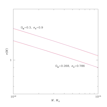
The scales corresponding to the galaxy-sized objects are sufficiently small that the slope of the matter power spectrum and hence the mass dependence in is insensitive to the underlying cosmology (Bardeen et al., 1986). In a fairly broad range of parameters around the “concordance” cosmological model, we find that computed with the full transfer function (e.g., Eisenstein & Hu, 1998) can be approximated as in the mass range . The amplitude, , of this power law approximation scales with cosmology as
| (A2) |
In this equation, the factor represents the correction for the different power spectrum shapes in different cosmologies (it is mostly a function of the product , see Bond & Efstathiou, 1984). We neglected such a factor in because we consider the cosmological models in which the perturbations are normalized by , the fluctuation amplitude at approximately the midpoint of the observed range. However, the scale corresponding to galaxy-sized objects for which has to be computed, is sufficiently far from Mpc so that the correction can be important. For example, we find that for the flat CDM cosmologies with and (more power in the high- case).
A.3. Scaling for
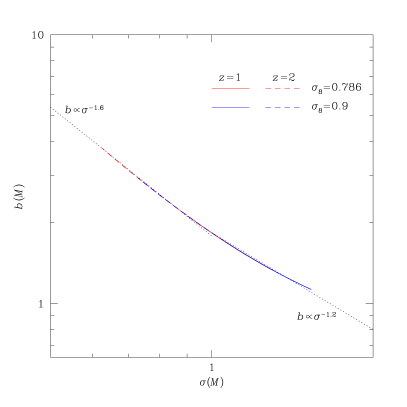
The key notion for our computation is that the halos with are “rare” objects at ( or less) with high bias factors strongly dependent on . The bias as a function of can be computed using the Sheth & Tormen (1999) approximation:
| (A3) |
with parameters and (adopted from Hu & Kravtsov, 2003, see their page 704), and is the threshold for spherical collapse in a matter-dominated universe. The bias computed from this equation for the two cosmologies and two different redshifts is shown in the right panel of Fig. 15. For the mass range , the bias can be approximated as at and at .
A.4. Scaling of Mass Derived from the Two-Point Correlation Functions
Since is a weak function of mass, the linear bias is also a weak function of , in our mass range. However, scales linearly with , and the bias also shows a strong dependence on this parameter, . For the correlation function of halos, we have . We, therefore, arrive at a somewhat counterintuitive conclusion — the amplitude of the correlation function of galaxy-sized objects at high is lower for models with high values of because of a strong dependence of the linear bias on the underlying amplitude of the density perturbations, .
When we determine the mass scale of objects from their correlation function, we effectively solve the equation
| (A4) |
where is a constant provided by the data. Inserting the scalings derived above, we can rewrite this as
| (A5) |
where we assume that is approximated as a power law of , (e.g., for our mass range and ). From here we have,
| (A6) |
If we scale the object masses by this equation, the halo clustering properties in the two different cosmologies will be very similar.
As an example, consider the scaling between the cosmology used in the simulations, , , , and the galaxy cluster-normalized best-fit model from Vikhlinin et al. (2009), , , . At , the median redshift of our Chandra/Boötes X-ray sample of AGNs, and for and 0.3, respectively. The shape factors, , are 1 and 1.03 for and 0.3, respectively. Inserting into eq. A6, we find that the masses which would be derived in the , cosmology are a factor of 1.45 lower than those derived using the correlation function models obtained directly from the simulation outputs.
A.5. Scaling for the Number Density of Objects
A related question is how to scale the number density of objects with the given clustering properties. In many situations, it should be possible to use a mass function model (e.g., the one from Sheth & Tormen, 1999) for such a scaling. However, for galaxy-sized objects it is possible to derive a simple scaling for the number density.
Jenkins et al. (2001) show that the mass function of halos can be written in a standard form,
| (A7) |
where is a constant, is the linear perturbations amplitude on scale , and is a “universal” function. For the Sheth & Tormen (1999) model,
| (A8) |
where the parameters and are the same as in the expression for the linear bias (eq. [A3]). For , as is the case for our galaxy-sized objects, the Sheth & Tormen is a slowly varying function of which can be approximated as
| (A9) |
Inserting this into eq. [A7] and taking into account that (see above), we have for the number density of objects above a mass threshold ,
| (A10) |
where . Now we can take into account that the limiting mass is found from the condition A4 (so that the clustering properties match those observed). If bias is approximated as a power law of , (Fig. 15),
| (A11) |
Equations A10, A11, and A6 provide the scaling for the number density of isolated halos whose clustering properties match the observations. Assuming that the relative number density of satellite and main halos is not very sensitive to the underlying cosmology, the same scaling can be applied to any other type of halos.
In summary, we suggest the following procedure. One takes the simulation outputs and adjusts the mass threshold, so that the correlation function amplitude derived for the halos with mass above this threshold matches that observed. One then measures the number density, , of such halos in the simulation box. To convert these quantities to the desired cosmology, one uses eq. A6 to scale and equations A10, A11, and A6 for the number density. For example, we found for the Chandra/Boötes AGNs km s-1, which corresponds to . This corresponds to at . To adjust these results from the to cosmology, we need to scale by a factor of 0.69, and increase the number density by a factor of 1.2 (the factor is partially compensated for by the change in ).