Task Release Control for Decision Making Queues

Abstract

We consider the optimal duration allocation in a decision making queue. Decision making tasks arrive at a given rate to a human operator. The correctness of the decision made by human evolves as a sigmoidal function of the duration allocated to the task. Each task in the queue loses its value continuously. We elucidate on this trade-off and determine optimal policies for the human operator. We show the optimal policy requires the human to drop some tasks. We present a receding horizon optimization strategy, and compare it with the greedy policy.

I Introduction

The advent of cheap camera sensors, has prompted the extensive deployment of camera sensor networks for surveillance [5, 9]. Typically, the feeds of these cameras are send to a central location, where a human operator looks at these feeds and decides on the existence of certain features. The correctness of the decision on a particular feed depends on the time-duration the human operator allocates to it. Thus, for a busy human operator, the optimal time-duration allocation is critically important.

Recently, there has been significant interest in understanding the physics of human decision making [3]. Several mathematical models for human decision making have been proposed [3, 13]. These models suggest that the correctness of the decision of a human operator in a binary decision making scenario evolves as a sigmoidal function of the time-duration allocated for decision. Thus, the probability of the correct decision by a human operator remains small till a critical time, and then jumps to a larger value. When a human operator has to serve a queue of decision making tasks, then the tasks (e.g., feeds from camera) waiting in the queue lose value continuously. This trade-off between the correctness of the decision and the loss in the value of the pending tasks is of critical importance for the performance of the human operator. In this paper, we address this trade-off, and determine optimal duration allocation policies for the human operator serving a decision making queue. Alternatively, we determine the task release rate that yields the desired accuracy for each task.

There has been a significant interest in the study of the performance of a human operator serving a queue. Schmidt [18] model the human as a server and numerically study a queueing model to determine the performance of a human air traffic controller. Maximally stabilizing task release policies for a human in the loop queue has been studied by Savla et al [14, 15, 16]. Bertuccelli et al [1] and Savla et al [17] study the human supervisory control for the unmanned aerial vehicle operations. Donohue et al [8] study an optimal duration allocation problem is a time constrained static queue.

The optimal control of queueing systems [19] is a classical problem in queueing theory. Stidham et al [12] study the optimal service policies for a M/G/1 queue. They formulate a semi-Markov decision process, and describe the qualitative features of the solution. Certain assumptions in [12] are relaxed by George et al [10]. Hernádez-Lerma et al [11] study an optimal adaptive service rate control policy for a M/G/1 queue with an unknown arrival rate.

We study the problem of optimal time-duration allocation in a queue of binary decision making tasks with a human operator. We refer to such queues as decision making queues. We consider three particular problems. First, we consider a time constrained static queue, where the human operator has to perform a given number of tasks with in a prescribed time. Second, we consider a static queue with latency penalty. Here, the human operator has to perform a given number of tasks. The operator incurs a penalty due to the delay in processing of each task. This penalty can be thought of as the loss in the value of the task over time. Last, we consider a dynamic queue of the decision making tasks. The tasks arrive at a fixed rate and the operator incurs a penalty for the delay in processing of each task. In all the three problems, there is a trade-off between the reward obtained by processing a task, and the penalty incurred due to resulting delay in processing other tasks. We address this particular trade-off. Major contributions of this work are:

1. We determine a closed form optimal duration allocation policy for the time constrained static decision making queue and the static decision making queue with penalty.

2. We provide a simple procedure to determine an optimal duration allocation policy for the dynamic decision making queue.

3. We rigorously establish that the optimal duration allocation policy may drop some tasks, i.e, not process the tasks at all.

The remainder of the paper is organized in the following way. We discuss some preliminary concepts in Section II. We present the problem setup in Section III. We present the optimal allocation policy for time constrained static queue in Section IV. The static queue with latency penalty is considered in Section V. We present the optimal allocation policy for the dynamic queue with latency penalty in Section VI. We elucidate on these problems further through some examples in Section VII. Our conclusions are presented in Section VIII.

II Preliminaries

II-A Speed-accuracy trade-off in human decision making

Consider the scenario where the human has to decide on one of the two alternatives $H_{0}$ and $H_{1}$, based on the collected evidence. The evolution of the probability of correct decision has been studied in cognitive psychology literature [2, 13, 3].

The probability of deciding on hypothesis $H_{1}$, given that hypothesis $H_{1}$ is true, at a given time $t\in\mathbb{R}_{\geq 0}$ is given by

$$\mathbb{P}(\text{say }H_{1}|H_{1},t)=\frac{p_{0}}{1+e^{-(at-b)}},$$

where $p_{0}\in[0,1]$, $a,b\in\mathbb{R}$ are some parameters which depend on the human operator [2, 13].

Conditioned on the hypothesis $H_{1}$, the evolution of the evidence for decision is modeled as a drift-diffusion process [3]. Given a drift rate $\beta>0$, and diffusion rate $\sigma$, with a decision threshold $\eta$, the conditional probability of the correct decision is

$$\mathbb{P}(\text{say }H_{1}|H_{1},t)=\frac{1}{\sqrt{2\pi\sigma^{2}t}}\int_{\eta}^{\infty}e^{\frac{-(\Lambda-\beta t)^{2}}{2\sigma^{2}t}}d\Lambda,$$

where $\Lambda\equiv\mathcal{N}(\beta t,\sigma^{2}t)$ is the evidence at time $t$.

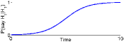
(a) Pew’s model

(b) Drift diffusion model

Figure 1: The sigmoidal evolution of the probabilities of correct decision

II-B Sigmoidal functions

A smooth function $f:\mathbb{R}_{\geq 0}\rightarrow\mathbb{R}_{\geq 0}$ defined by

$$f(t)=f_{\text{cvx}}(t)\mathcal{I}(t<t_{\text{inf}})+f_{\text{cnv}}(t)\mathcal{I}(t\geq t_{\text{inf}}),$$

where $f_{\text{cvx}}$ and $f_{\text{cnv}}$ are monotonically increasing convex and concave functions, respectively, and $t_{\text{inf}}$ is the inflection point. Derivative of sigmoidal function is unimodal with maximum at $t_{\text{inf}}$. Further, $f^{\prime}(0)\geq 0$ and $\lim_{t\to\infty}f^{\prime}(t)=0.$ Also, $\lim_{t\to\infty}f^{\prime\prime}(t)=0.$ A typical graph of the first and second derivative of a sigmoidal function is shown in Figure 2. Note that the evolution of the conditional probabilities of correct decision are sigmoidal functions in Pew’s as well as drift-diffusion model.

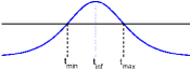
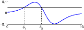
Figure 2: (a) First derivative of the sigmoidal function and penalty rate. A particular value of the derivative may be attained at two different times. The total benefit decreases till $t_{\min}$, increases from $t_{\min}$ to $t_{\max}$, and then decreases again. (b) Second derivative of the sigmoidal function. A particular positive value of the second derivative may be attained at two different times.

II-C Receding horizon optimization

Consider the following infinite horizon dynamic optimization problem.

$$\begin{split}\text{maximize}&\quad\sum_{\ell=1}^{\infty}\psi(x(\ell),u(\ell))\\ \text{subject to}&\quad x(\ell+1)=\phi(x(\ell),u(\ell)),\end{split}$$ (1)

where $x(\ell),u(\ell)\in\mathbb{R}$ are the state and control input at time $\ell\in\mathbb{N}$, respectively, $\psi:\mathbb{R}\times\mathbb{R}\rightarrow\mathbb{R}$ is the stage cost, and $\phi:\mathbb{R}\times\mathbb{R}\rightarrow\mathbb{R}$ defines the nonlinear evolution of the system.

The receding horizon optimization [6] approximates the optimization problem (1) as the following finite horizon optimization problem at each stage $\theta\in\mathbb{N}$:

$$\begin{split}\text{maximize}&\quad\sum_{\ell=\theta}^{\theta+N}\psi(x(\ell),u(\ell))\\ \text{subject to}&\quad x(\ell+1)=\phi(x(\ell),u(\ell)),\end{split}$$ (2)

where $N\in\mathbb{N}$ is a finite horizon length. The receding horizon optimization is summarized as following

Algorithm 1 Receding horizon optimization

1:  at time $\theta\in\mathbb{N}$, observe state $x(\theta)$

2:  Solve optimal control problem (2) and compute the optimal control inputs $u^{*}(\theta),\ldots,u^{*}(\theta+T)$

3:  Apply $u^{*}(\theta)$, and set $\theta=\theta+1$

4:  Go to step 1:

III Problem setup

We consider the problem of optimal time duration allocation for a human operator. The decision making tasks arrive at a given rate and are processed by a human operator (see Figure 3.) The human receives a unit reward for the correct decision, while there is no penalty for a wrong decision. For a decision made at time $t$, the expected reward is

$$\mathbb{E}[\boldsymbol{1}_{\text{say }H_{1}|H_{1},t}]=\mathbb{P}(\text{say }H_{1}|H_{1},t)=f(t),$$ (3)

where $f:\mathbb{R}_{\geq 0}\rightarrow[0,1]$ is a sigmoidal function.

We consider three particular problems. First, we consider a time constrained static queue, i.e., the human operator has to perform $N\in\mathbb{N}$ identical decision making tasks with in time $T\in\mathbb{R}_{>0}$. Second, we consider a static queue with penalty, i.e., the human operator has to perform $N\in\mathbb{N}$ identical decision making tasks, but each task lose value at a constant rate per unit delay in its processing. Last, we consider a dynamic queue of identical decision making tasks where each task lose value at a constant rate per unit delay in its processing. For such a decision making queue, we are interested in the optimal time-duration allocation to each task. Alternatively, we are interested in the task release rate that will result in the desired accuracy for each task. We intend to design a decision support system that tells the human operator the optimal time-duration allocation for each task.

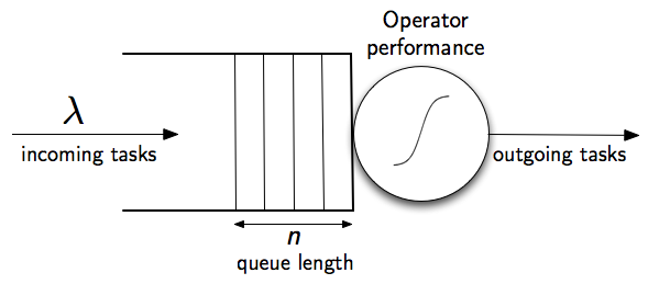
Figure 3: Problem setup. The decision making tasks arrive at a rate $\lambda$. These tasks are served by a human operator with sigmoidal performance. Each task loses value while waiting in the queue.

IV Time constrained static queue

IV-A Problem description

Consider that the human operator has to perform $N\in\mathbb{N}$ identical tasks with in time $T\in\mathbb{R}_{>0}$. Let the human operator allocates duration $t_{\ell}$ to the task $\ell\in\{1,\dots,N\}$. The following optimization problem encapsulates the objective of the human operator:

$$\begin{split}\underset{\boldsymbol{t}}{\text{maximize}}&\quad\sum_{\ell=1}^{N}f(t_{\ell})\\ \text{subject to}&\quad\sum_{\ell=1}^{N}t_{\ell}\leq T\\ &\quad\boldsymbol{t}\succeq 0,\end{split}$$ (4)

where $\boldsymbol{t}=\{t_{1},\dots,t_{N}\}$ is the duration allocation vector.

IV-B Optimal policy

We define the Lagrangian $L:\mathbb{R}^{N}_{>0}\times\mathbb{R}_{\geq 0}\times\mathbb{R}^{N}_{\geq 0}\rightarrow\mathbb{R}$ for the constrained optimization problem (4) by

$$L(\boldsymbol{t},\alpha,\boldsymbol{\mu})=\sum_{\ell=1}^{N}f(t_{\ell})+\alpha(T-\sum_{\ell=1}^{N}t_{\ell})+\boldsymbol{\mu}^{\text{T}}\boldsymbol{t}.$$

We also define the dual cost function $h:\mathbb{R}_{\geq 0}\times\mathbb{R}^{N}_{\geq 0}\rightarrow\mathbb{R}$ by

$$h(\alpha,\boldsymbol{\mu})=\underset{\boldsymbol{t}\in\mathbb{R}^{N}_{\geq 0}}{\max}L(\boldsymbol{t},\alpha,\boldsymbol{\mu}).$$ (5)

The dual problem to the primal optimization problem (4) is

$$\begin{split}\text{minimize}&\quad h(\alpha,\boldsymbol{\mu})\\ \text{subject to}&\quad\alpha\geq 0,\;\boldsymbol{\mu}\succeq 0.\end{split}$$ (6)

Lemma 1 (Constraint qualification)

For the primal problem (4) and the dual problem (6), the constraint qualification holds.

Proof:

Let $\boldsymbol{t}^{*}$ be an optimal solution to the primal problem (4). Without loss of generality assume that $t^{*}_{1}>0$, i.e., $t^{*}_{1}\geq 0$ is not an active constraint. The gradients of the other constraints are $\boldsymbol{e}_{j}$, $j\in\{2,\ldots,N\}$ and $\boldsymbol{1}_{N}$, where $\boldsymbol{e}_{j}$ is the ${j}^{\text{th}}$ standard Cartesian unit vector, and $\boldsymbol{1}_{N}$ is the $N$-tuple with all ones. It immediately follows that these gradients are linearly independent. Thus, the constraint qualification [7] holds. ∎

Theorem 2 (Time constrained static queue)

For the optimization problem (4), the optimal duration allocation vector $\boldsymbol{t}^{*}$ is an $N$-tuple with $m^{*}$ entries equal to $T/m^{*}$ and all other entries zero, where

$$m^{*}=\underset{m\in\{1,\dots,N\}}{\operatorname{argmax}}mf(T/m).$$

Proof:

We apply the Karush-Kuhn-Tucker necessary conditions [4] for an optimal solution $\boldsymbol{t}^{*},\alpha^{*},\boldsymbol{\mu}^{*}$.
Linear dependence of gradients

$$\frac{\partial L}{\partial t^{*}_{\ell}}(\boldsymbol{t}^{*},\alpha^{*},\boldsymbol{\mu}^{*})=f^{\prime}(t^{*}_{\ell})-\alpha^{*}+\mu^{*}_{\ell}=0,\\ \forall\ell\in\{1,\dots,N\}.$$ (7)

Feasibility of the solution

$$T-\boldsymbol{1}_{N}^{\text{T}}\boldsymbol{t}^{*} \geq 0.$$ (8)

$$\boldsymbol{t}^{*} \succeq 0.$$ (9)

Complementarity conditions

$$\alpha^{*}(T-\boldsymbol{1}_{N}^{\text{T}}\boldsymbol{t}^{*}) =0.$$ (10)

$$\mu_{\ell}^{*}t^{*}_{\ell} =0,\;\forall\ell\in\{1,\dots,N\}.$$ (11)

Non-negativity of the multipliers

$$\alpha^{*}\geq 0,\quad\boldsymbol{\mu}^{*}\succeq 0.$$ (12)

Since $f$ is a strictly increasing function, the constraint (8) should be active, and thus, from complementarity condition (10) $\alpha^{*}>0$. Further, from equation (11), if $t^{*}_{\ell}\neq 0$, then $\mu_{\ell}^{*}=0$. Assume that $t^{*}_{\ell}\neq 0$, then, for each $\ell\in\{1,\dots,N\}$, the equation (7) yields

$$f^{\prime}(t^{*}_{\ell})=\alpha^{*}.$$ (13)

If the equation (13) has no solution, then the Lagrangian is decreasing function of $t^{*}_{\ell}$, and the optimal duration allocation is zero. But $t^{*}_{\ell}\neq 0$, by assumption. Thus, there exists a solution of equation (13). Since, the derivative of a sigmoidal function is uni-modal, there exists two solutions of equation (13). We refer to these values of $t^{*}_{\ell}$ as $t^{-}$ and $t^{+}$, with the understanding that $t^{+}\geq t^{-}$. From Figure 2, it follows that a local minima exists at $t^{-}$, while a local maxima exists at $t^{+}$. Further note that the Lagrangian is a decoupled function of $t_{\ell},\;\ell\in\{1,\dots,N\}$. Thus, the optimal $\boldsymbol{t}^{*}$ will contain no $t^{-}$ entry. Moreover, each entry will be either zero or $t^{+}$. Let $m^{*}\leq N$ entries of optimal $\boldsymbol{t}^{*}$ be non-zero. Any allocation with $m$ identical non-zero entries, and remaining zero entries yields a reward $mf(T/m)$. Therefore, the optimal non-zero entries are as stated in the theorem. ∎

Remark 3 (Notes on concavity I)

If the performance function $f$ is a concave function, the optimal policy for the time constrained queue is to allocate equal time to each task. $\square$

V Static queue with latency penalty

V-A Problem description

Consider that the human operator has to perform $N\in\mathbb{N}$ identical tasks. Let the human operator assigns time $t_{\ell}$ to the task $\ell\in\{1,\dots,N\}$. The operator receives an expected reward $f(t_{\ell})$ for an assignment $t_{\ell}$ to the task $\ell$, while she incurs a latency cost $c$ per unit time for the delay in processing of each task. The following optimization problem encapsulates the objective of the human operator:

$$\underset{\boldsymbol{t}\succeq 0}{\text{maximize}}\quad\frac{1}{N}\sum_{\ell=1}^{N}\big{(}f(t_{\ell})-ct_{\ell}(N-\ell+1)\big{)},\\$$ (14)

where $\boldsymbol{t}=\{t_{1},\dots,t_{N}\}$ is the duration allocation vector.

V-B Optimal policy

Theorem 4 (Static queue with latency penalty)

For the optimization problem (14), the optimal allocation at stage $\ell\in\{1,\dots,N\}$ is

$$t^{*}_{\ell} :=\underset{\beta\in\{0,t^{{\dagger}}_{\ell}\}}{\operatorname{argmax}}\big{(}f(\beta)-c(N\!-\ell\!+1)\beta\big{)},$$

where

$$t^{{\dagger}}_{\ell}:=\begin{cases}0,&\quad\text{if }f^{\prime}(t_{\text{inf}})<c(N\!-\!\ell\!+\!1),\\ \max\{t\in\mathbb{R}_{>0}\;|\;f^{\prime}(t)=\!\!&\!\!c(N\!-\ell\!+1)\},\quad\text{otherwise.}\end{cases}$$

Proof:

The proof is similar to the proof of Theorem 2. If $f^{\prime}(t_{\text{inf}})<c(N\!-\!\ell\!+\!1)$, then the objective is a decreasing function of $t_{\ell}$, and the optimal allocation is zero. Otherwise, the local maximum lies at the intersection of penalty rate $c(N-\ell+1)$ with the decreasing portion of the $f^{\prime}$ (see Figure 2). The optimal allocation $t^{*}_{\ell}$ is determined by comparing value of the objective function at the local maxima and the boundary. ∎

Remark 5 (Notes on concavity II)

The optimal duration allocation for the static queue with latency penalty decreases to a critical value $t_{\text{crit}}>t_{\text{inf}}$ with increasing penalty rate, then jumps down to zero. Instead, if the performance function $f$ is concave, then the optimal duration allocation decreases continuously to zero with increasing penalty rate. $\square$

VI Dynamic queue with latency penalty

VI-A Problem description

Consider that the human operator has to serve a queue of identical decision making tasks. Assume that the tasks arrive as a Poisson’s process with rate $\lambda>0$. We define the processing of job $\ell\in\mathbb{N}$ as the stage $\ell$. Let the operator assign deterministic time $t_{\ell}$ at stage $\ell$. The operator receives an expected reward $f(t_{\ell})$ for a duration allocation $t_{\ell}$ at stage $\ell$, while she incurs a latency cost $c$ per unit time for the delay in processing each task. We denote the queue length at stage $\ell$ by $n_{\ell}$. The objective of the operator is to maximize her infinite horizon expected reward. The following optimization problem encapsulates the objective of the human operator:

$$\begin{split}{\text{maximize}}&\quad\lim_{L\to\infty}\frac{1}{L}\sum_{\ell=1}^{L}\Big{(}f(t_{\ell})-c\mathbb{E}[n_{\ell}]t_{\ell}-\frac{c\lambda t_{\ell}^{2}}{2}\Big{)}\\ \text{subject to}&\quad\mathbb{E}[n_{\ell+1}]=\max\{0,\mathbb{E}[n_{\ell}]-1+\lambda t_{\ell}\}\\ &\quad t_{\ell}\geq 0,\forall\ell\in\mathbb{N},\end{split}$$ (15)

where the term $c\lambda t_{\ell}^{2}/2$ is the expected penalty due to the tasks arriving during stage $\ell$.

VI-B Optimal policy

Finite horizon optimization

We wish to approximately solve the infinite horizon optimization problem (15) using receding horizon optimization as in Algorithm 1. To do so, we pose the following finite horizon optimization problem:

$$\begin{split}\underset{\boldsymbol{t}\succeq 0}{\text{maximize}}&\quad\frac{1}{N}\sum_{\ell=1}^{N}\Big{(}f(t_{\ell})-c\mathbb{E}[n_{\ell}]t_{\ell}-\frac{c\lambda t_{\ell}^{2}}{2}\Big{)}\\ \text{subject to}&\quad\mathbb{E}[n_{\ell+1}]=\max\{0,\mathbb{E}[n_{\ell}]-1+\lambda t_{\ell}\},\end{split}$$ (16)

where $\boldsymbol{t}=\{t_{1},\dots,t_{N}\}$ is the duration allocation vector.

Without loss of generality, we assume that the queue length is always non-zero. If the queue is empty at some time, then the operator will wait till the arrival of new task. There is no explicit penalty for the operator to be idle. Under this assumption we have

$$\mathbb{E}[n_{\ell}]=n_{1}-\ell+1+\lambda\sum_{j=1}^{\ell-1}t_{j}.$$

Some algebraic manipulations show that the objective function of the optimization problem (16) is equivalent to the function $J:\mathbb{R}_{\geq 0}^{N}\rightarrow\mathbb{R}$ defined by

$$J(\boldsymbol{t}):=\frac{1}{N}\sum_{\ell=1}^{N}\Big{(}f(t_{\ell})-c(n_{1}-\ell+1)t_{\ell}-c\lambda t_{\ell}\sum_{j=1}^{N}t_{j}+\frac{c\lambda t_{\ell}^{2}}{2}\Big{)},$$

where $c$ is the penalty rate, $\lambda$ is the arrival rate, and $n_{1}$ is the initial queue length. Thus, the optimization problem (16) is equivalent to

$$\underset{\boldsymbol{t}\succeq 0}{\text{maximize}}\quad J(\boldsymbol{t}).$$ (17)

We define $f^{\prime}_{\text{inv}}:[0,f^{\prime}(t_{\text{inf}})]\rightarrow\mathbb{R}_{\geq 0}$ by

$$f^{\prime}_{\text{inv}}(y)=\max\{t\in\mathbb{R}_{\geq 0}\;|\;f(t)=y\}.$$

Note that the definition of $f^{\prime}_{\text{inv}}$ is consistent with Figure 2.

For the optimization problem (16), assume that the optimal policy allocates a strictly positive time only to the tasks in the set $\mathcal{T}_{\textup{processed}}\subseteq\{1,\dots,N\}$, which we call the set of processed tasks. (Accordingly, the policy allocates zero time to the tasks in $\{1,\dots,N\}\setminus\mathcal{T}_{\textup{processed}}$). Without loss of generality, assume

$$\mathcal{T}_{\textup{processed}}:=\{\eta_{1},\ldots,\eta_{m}\},$$

where $\eta_{1}<\cdots<\eta_{m}$ and $m\leq N$. A duration allocation vector $\boldsymbol{t}$ is said to be consistent with $\mathcal{T}_{\textup{processed}}$ if only the tasks in $\mathcal{T}_{\textup{processed}}$ are allocated non-zero duration.

Lemma 6 (Properties of maximum point)

For the optimization problem (17), and a set of processed tasks $\mathcal{T}_{\textup{processed}}$, the following statements hold:

1. A global maximum point $\boldsymbol{t}^{*}$ satisfy $t^{*}_{\eta_{j}}\geq t^{*}_{\eta_{k}}$, for $j\geq k$, $j,k\in\{1,\dots,m\}$.

2. A local maximum point $\boldsymbol{t}^{{\dagger}}$ consistent with $\mathcal{T}_{\textup{processed}}$ satisfies

   $$f^{\prime}(t_{\eta_{k}}^{{\dagger}})=c(n_{1}-\eta_{k}+1)+c\lambda\sum_{i=1}^{m}t^{{\dagger}}_{\eta_{i}},\forall k\in\{1,\dots,m\}.$$ (18)

3. The system on equations (18), can be reduced to

   $$f^{\prime}(t_{\eta_{1}}^{\dagger})=\mathcal{P}(t_{\eta_{1}}^{\dagger}),\text{ and }t^{\dagger}_{\eta_{k}}=f^{\prime}_{\text{inv}}(f^{\prime}(t_{\eta_{1}}^{\dagger})-c(\eta_{k}-\eta_{1})),$$

   for each $k\in\{2,\dots,m\}$, where $\mathcal{P}:\mathbb{R}_{>0}\rightarrow\mathbb{R}\operatorname{\cup}\{+\infty\}$ is defined by

   $$\mathcal{P}(t)=\begin{cases}p(t),\quad&\text{if }f^{\prime}(t)\geq c(\eta_{m}-\eta_{1}),\\ +\infty,&\text{otherwise,}\end{cases}$$

   where
   $\displaystyle p(t)\!=\!c\Big{(}\!n_{1}-\eta_{1}+1+\lambda t+\lambda\!\sum_{k=2}^{m}\!f^{\prime}_{\text{inv}}\!\big{(}f^{\prime}(t)-c(\eta_{k}-\eta_{1})\!\big{)}\!\Big{)}$.

4. A local maximum point $\boldsymbol{t}^{{\dagger}}$ consistent with $\mathcal{T}_{\textup{processed}}$ satisfies

   $$f^{\prime\prime}(t_{\eta_{k}})\leq c\lambda,\text{ for each }k\in\{1,\dots,m\}.$$

Proof:

We start by proving the first statement. Assume $t_{\eta_{j}}^{*}<t_{\eta_{k}}^{*}$ and define the allocation vector $\bar{\boldsymbol{t}}$ consistent with $\mathcal{T}_{\textup{processed}}$ by

$$\bar{t}_{\eta_{i}}=\begin{cases}t^{*}_{\eta_{i}},&\text{if }i\in\{1,\dots,m\}\setminus\{j,k\},\\ t^{*}_{\eta_{j}},&\text{if }i=k,\\ t^{*}_{\eta_{k}},&\text{if }i=j.\end{cases}$$

It is easy to see that

$$J(\boldsymbol{t}^{*})-J(\bar{\boldsymbol{t}})=(\eta_{j}-\eta_{k})(t_{\eta_{j}}^{*}-t_{\eta_{k}}^{*})<0.$$

This inequality contradicts the assumption that $\boldsymbol{t}^{*}$ is a solution of the optimization problem (17).

To prove the second statement, note that a local maximum is achieved at the boundary of the feasible region or at the set where the Jacobian of $J$ is zero. At the boundary of the feasible region $\mathbb{R}^{N}_{\geq 0}$, some of the allocations are zero. Given the $m$ non-zero allocations, the Jacobian of the function $J$ projected on the space spanned by the non-zero allocations must be zero. The expressions in the theorem are obtained by setting the Jacobian to zero.

To prove the third statement, we subtract, the expression in equation (18) for $k=j$ from the expression for $k=1$ to get

$$f^{\prime}(t_{\eta_{j}})=f^{\prime}(t_{\eta_{1}})-c(\eta_{j}-\eta_{1}).$$ (19)

There exists a solution of equation (19) if and only if $f^{\prime}(t_{\eta_{1}})\geq c(\eta_{j}-\eta_{1})$. If $f^{\prime}(t_{\eta_{1}})<c(\eta_{j}-\eta_{1})+f^{\prime}(0)$, then there exists only one solution. Otherwise, there exist two solutions. It can be seen that if there exist two solutions $t^{\pm}_{j}$, $t_{j}^{-}<t_{j}^{+}$, then $t_{j}^{-}<t_{\eta_{1}}<t_{j}^{+}$. From i), only possible allocation is $t_{j}^{+}$. Notice that $t_{j}^{+}=f^{\prime}_{\text{inv}}(f^{\prime}(t_{\eta_{1}})-c(\eta_{j}-\eta_{1}))$. This yields feasible time allocation to each task $\eta_{j},j\in\{2,\ldots,m\}$ parametrized by the time allocation to the task $\eta_{1}$. A typical allocation is shown in Figure 4. We further note that the effective penalty rate for the task $\eta_{1}$ is $c(n_{1}-\eta_{1}+1)+c\lambda\sum_{j=1}^{m}t_{\eta_{j}}$. Using the expression of $t_{\eta_{j}},j\in\{2,\ldots,m\}$, parametrized by $t_{\eta_{1}}$, we obtain the expression for $\mathcal{P}$.

To prove the last statement, we observe that the Hessian of the function $J$ is

$$\frac{\partial^{2}J}{\partial\boldsymbol{t}^{2}}=\text{diag}(f^{\prime\prime}(t_{\eta_{1}}),\ldots,f^{\prime\prime}(t_{\eta_{m}}))-c\lambda\boldsymbol{1}_{m}\boldsymbol{1}_{m}^{T},$$

where $\text{diag}(\cdot)$ represents a diagonal matrix with the argument as diagonal entries. For a local maximum to exist at non-zero duration allocations $\{t_{\eta_{1}},\dots,t_{\eta_{m}}\}$, the Hessian must be negative semidefinite. Thus, a necessary condition for Hessian to be negative semidefinite is that diagonal entries are non-positive. ∎

We refer to the function $\mathcal{P}$ by the effective penalty rate for the first processed task. A typical graph of $\mathcal{P}$ is shown in Figure 4. Given $\mathcal{T}_{\textup{processed}}$, a feasible allocation to the task $\eta_{1}$ is such that $f(t_{\eta_{1}})-c(\eta_{j}-\eta_{1})>0$, for each $j\in\{2,\dots,m\}$. For a given $\mathcal{T}_{\textup{processed}}$, we define the minimum feasible duration allocated to task $\eta_{1}$ (see Figure 4) by

$$\tau_{1}\!:=\!\begin{cases}\!\min\{t\!\in\!\mathbb{R}_{\!\geq\!0\!}\!\;|\;\!f^{\prime}\!(t)\!=\!c(\!\eta_{m}\!-\!\eta_{1}\!)\!\},&\!\text{if }\!f^{\prime}\!(\!t_{\text{inf}}\!)\!\geq\!c(\!\eta_{m}\!-\!\eta_{1}\!),\\ 0,&\!\text{otherwise.}\end{cases}$$

Let $f^{\prime\prime}_{\text{max}}$ be the maximum value of $f^{\prime\prime}$. We now define the points at which the function $f^{\prime\prime}-c\lambda$ changes its sign (see Figure 2):

$$\delta_{1} :=\begin{cases}\min\{t\in\mathbb{R}_{\geq 0}\;|\;f^{\prime\prime}(t)=c\lambda\},&\text{if }c\lambda\in[f^{\prime\prime}(0),f^{\prime\prime}_{\text{max}}],\\ 0,&\text{otherwise,}\end{cases}$$

$$\delta_{2} :=\begin{cases}\max\{t\in\mathbb{R}_{\geq 0}\;|\;f^{\prime\prime}(t)=c\lambda\},&\text{if }c\lambda\leq f^{\prime\prime}_{\text{max}},\\ 0,&\text{otherwise.}\end{cases}$$

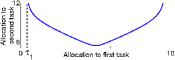
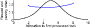
Figure 4: (a) Feasible allocations to second task parametrized by allocation to first task. (b) The penalty rate and the reward rate due to the allocation to the first task.

Theorem 7 (Dynamic queue with latency penalty)

For the optimization problem (17), consider a set of processed tasks $\mathcal{T}_{\textup{processed}}$. The following statements hold:

1. there exists a local maximum point consistent with $\mathcal{T}_{\textup{processed}}$, if

   $$f^{\prime}(\delta_{2}) \geq\mathcal{P}(\delta_{2});$$ (20)

2. there exists a local maximum point consistent with $\mathcal{T}_{\textup{processed}}$, if

   $$f^{\prime}(\tau_{1}) \leq\mathcal{P}(\tau_{1}),\;f^{\prime}(\delta_{1})\geq\mathcal{P}(\delta_{1}),\;\text{and }\delta_{1}\geq\tau_{1};$$ (21)

3. if both conditions (20) and (21) are false, then there exist no local maximum point consistent with $\mathcal{T}_{\textup{processed}}$.

Proof:

A critical allocation to task $\eta_{1}$ is located at the intersection of the graph of the reward rate function $f^{\prime}(t_{\eta_{1}})$ to the penalty functions $\mathcal{P}(t_{\eta_{1}})$. From Lemma 6, a necessary condition for existence of local maximum at a critical point is $f^{\prime\prime}(t_{\eta_{1}})\leq c\lambda$ . Further, for $t_{\eta_{1}}\in{]0,\delta_{1}]}\operatorname{\cup}{[\delta_{2},\infty[}$, $f^{\prime\prime}(t_{\eta_{1}})\leq c\lambda$. It can be seen that if condition (20) holds, then the reward function $f^{\prime}(t_{\eta_{1}})$ and the effective penalty function $\mathcal{P}(t_{\eta_{1}})$ intersect in the region ${[\delta_{2},\infty[}$. Similarly, condition (21) ensure the intersection of the graph of the reward function $f^{\prime}(t_{\eta_{1}})$ with the effective penalty function $\mathcal{P}(t_{\eta_{1}})$ in the region ${]0,\delta_{1}]}$. ∎

We now provide a procedure to provide solution to the optimization problem (16). Given a sequence of zero and non-zero allocations $\xi\in\{0,+\}^{N}$, we denote the corresponding critical allocation for maximum by $\boldsymbol{t}(\xi)$. The details of the procedure are shown in Algorithm 2.

Algorithm 2 Optimal allocation for decision making queue

1:  given $n_{1}$, $N$, $c$, $\lambda$

2:  $k:=0$; $\mathcal{A}:=\phi$;

3:  for each string $\xi\in\{0,+\}^{N}$

4:   set $\mathcal{T}_{\textup{processed}}:=\{i\in\{1,\dots,N\}\;|\;\xi_{i}=+\}$

5:   if condition (20) or (21)

6:   then determine critical allocations for maximum $t_{\eta_{1}}^{{\dagger}}$ via bisection algorithm

7:      determine allocations $t_{\eta_{j}}^{{\dagger}},j\in\{2,\ldots,m\}$

8:      determine expected queue lengths$\mathbb{E}[n_{\ell}],\ell\in\{1,\dots,N\}$

9:       if $\mathbb{E}[n_{\ell}]>0,\forall\ell\in\{1,\dots,N\}$

10:       then $\mathcal{A}=\mathcal{A}\operatorname{\cup}\{\boldsymbol{t}^{{\dagger}}(\xi)\}$

11:  optimal allocation $\boldsymbol{t}^{*}=\text{argmax}_{\boldsymbol{t}\in\mathcal{A}}J(\boldsymbol{t})$

Remark 8 (Notes on concavity III)

With the increasing penalty rate as well as the increasing arrival rate, the time duration allocation decreases to a critical value $t_{\text{crit}}>t_{\text{inf}}$ and then jumps down to zero, for the dynamic queue with latency penalty. Instead, if the performance function $f$ is concave, then the duration allocation decreases continuously to zero with increasing penalty rate as well as increasing arrival rate. $\square$

VII Numerical examples

We now elucidate on the optimal policies for the three problems through some numerical examples. We consider three examples. In the first and second example, we demonstrate application of Theorem 2 and 4, respectively. In the third example, the Algorithm 2 is utilized in a receding horizon fashion.

Example 9

If the human operator has to serve $N=10$ tasks in time $T=30$ secs, and the human receives an expected reward $f(t)=1/(1+\exp(5-t))$ for an allocation of duration $t$ secs to a task, then the optimal policy for the human is to drop six tasks, and allocate $7.5$ secs to any four tasks. An optimal allocation is shown in Figure 5(a). $\square$

Example 10

If the human operator has to serve $N=10$ tasks and the human receives an expected reward $f(t)=1/(1+\exp(5-t))$ for an allocation of duration $t$ secs to a task, while she incurs a penalty $c=0.02$ per sec for each pending task, then the optimal policy for the human is shown in Figure 5(b) . Note that the optimal duration allocation increases with decreasing number of pending tasks. $\square$

(a) Time constrained static queue

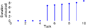
(b) Static queue wt. latency penalty

Figure 5: Optimal allocations

Example 11

If the human operator has to serve a queue of tasks with Poisson arrival at rate $\lambda=0.5$ per sec and the human receives an expected reward $f(t)=1/(1+\exp(5-t))$ for an allocation of duration $t$ secs to a task, while she incurs a penalty $c=0.01$ per sec for each task in queue. We solved an optimization problem with horizon length $N=10$ at each stage to determine the receding horizon optimization solution. A receding horizon policy for the expected evolution of the queue, at different arrival rates, is shown in Figure 6. A receding horizon duration allocation policy for a sample evolution of the queue, at different arrival rates, is shown in Figure 7. The duration allocations for a greedy policy, i.e., an optimization with horizon length $N=1$ at each stage, are shown in Figure 8. The optimal expected benefit $J(\boldsymbol{t})$ for the optimal and the greedy policy is shown in Figure 9. It can be seen that the maximum benefit is obtained at an arrival rate at which one expects only one task in the queue at each time. As expected, the performance of the greedy policy and the optimal policy is almost the same at this arrival rate. $\square$

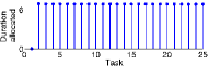
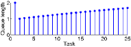
(a) Low arrival rate

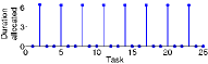
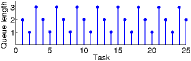
(b) Moderate arrival rate

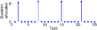
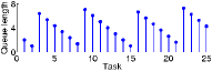
(c) High arrival rate

Figure 6: Receding horizon policy for expected evolution of the dynamic queue with latency penalty. An optimization problem with horizon length $N=10$ is solved at each stage.

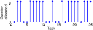
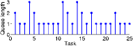
(a) Low arrival rate

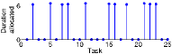
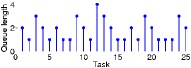
(b) Moderate arrival rate

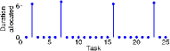
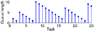
(c) High arrival rate

Figure 7: Receding horizon policy for a sample evolution of the dynamic queue with latency penalty. An optimization problem with horizon length $N=10$ is solved at each stage.

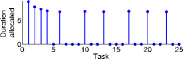
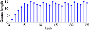
Figure 8: Greedy policy for the expected evolution of the dynamic queue with latency penalty. An optimization problem with horizon length $N=1$ is solved at each stage.

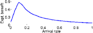
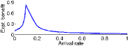
Figure 9: Expected benefit over a finite horizon for the receding horizon and greedy policies

Remark 12 (Optimal arrival rate)

It can be seen that the total expected benefit is maximum when there is always only one task in the queue. If there is more than one task in the queue, then the operator is incurring more penalty for the same reward. Thus, the optimal arrival is the one at which a task arrival is expected at the time when the previous task loses all its value, i.e., at $\tau^{*}=\max\{t\in\mathbb{R}_{\geq 0}\;|\;f^{\prime}(t)=2c\}$. In general, there would be performance goals for the operator, and higher task arrival rate for the queue could be designed. Such a problem can be analyzed by putting a saturation on the sigmoidal performance function, and thus obtaining a new sigmoidal performance function. $\square$

VIII Conclusions

We presented an analysis on the decision making queues. Three particular problems were discussed. First, a time constrained decision making queue with no arrival was considered. We showed that the optimal policy may drop some tasks and assign equal time to the remaining tasks. Second, a decision making queue with no arrival and a latency penalty was considered. It was observed that the optimal policy may still drop some tasks. Further, the duration allocation to the tasks increased with the decreasing queue length. Last, a decision making queue with latency penalty was considered. A receding horizon policy was developed to determine the optimal duration allocation. It was observed that the optimal policy may drop some tasks.

The decision support system designed in this paper assumes that the arrival rate of the tasks as well as the parameters in the performance function are known. An interesting open problem is to estimate the parameters of the performance function, and come up with policies which perform an online estimation of the arrival rate, and accordingly determine the optimal allocation policy.

References

- [1] L. F. Bertuccelli, N. Pellegrino, and M. L. Cummings. Choice modeling of relook tasks for UAV search missions. In American Control Conference, pages 2410–2415, Baltimore, MD, June 2010.
- [2] K. L. Boettcher and R. R. Tenney. Distributed decisionmaking with constrained decision makers. a case study. IEEE Transactions on Systems, Man & Cybernetics, 16(6):813–823, 1986.
- [3] R. Bogacz, E. Brown, J. Moehlis, P. Holmes, and J. D. Cohen. The physics of optimal decision making: A formal analysis of performance in two-alternative forced choice tasks. Psychological Review, 113(4):700–765, 2006.
- [4] S. Boyd and L. Vandenberghe. Convex Optimization. Cambridge University Press, 2004.
- [5] W. M. Bulkeley. Chicago’s camera network is everywhere. The Wall Street Journal, Nov 17 2009.
- [6] E. F. Camacho and C. Bordons. Model Predictive Control. Springer, 2004.
- [7] U. Diwekar. Introduction to Applied Optimization. Springer, 2008.
- [8] M. Donohue and C. Langbort. Tasking human agents: A sigmoidal utility maximization approach for target identification in mixed teams of humans and UAVs. In AIAA Conf. on Guidance, Navigation and Control, Chicago, IL, August 2009.
- [9] C. Drew. Military taps social networking skills. The New York Times, June, 7 2010.
- [10] J. M. George and J. M. Harrison. Dynamic control of a queue with adjustable service rate. Operations Research, 49(5):720–731, 2001.
- [11] O. Hernández-Lerma and S. I. Marcus. Adaptive control of service in queueing systems. Systems & Control Letters, 3(5):283–289, 1983.
- [12] S. Stidham Jr. and R. R. Weber. Monotonic and insensitive optimal policies for control of queues with undiscounted costs. Operations Research, 37(4):611–625, 1989.
- [13] R. W. Pew. The speed-accuracy operating characteristic. Acta Psychologica, 30:16–26, 1969.
- [14] K. Savla and E. Frazzoli. A dynamical queue approach to intelligent task management for human operators. Proceedings of the IEEE, 2010. submitted.
- [15] K. Savla and E. Frazzoli. Maximally stabilizing task release control policy for a dynamical queue. In American Control Conference, pages 2404–2409, Baltimore, MD, June 2010.
- [16] K. Savla and E. Frazzoli. Maximally stabilizing task release control policy for a dynamical queue. IEEE Transactions on Automatic Control, 55(11), 2010. to appear.
- [17] K. Savla, T. Temple, and E. Frazzoli. Human-in-the-loop vehicle routing policies for dynamic environments. In IEEE Conf. on Decision and Control, pages 1145–1150, Cancún, México, December 2008.
- [18] D. K. Schmidt. A queuing analysis of the air traffic controller’s work load. IEEE Transactions on Systems, Man & Cybernetics, 8(6):492–498, 1978.
- [19] L. I. Sennott. Stochastic Dynamic Programming and the Control of Queueing Systems. Wiley, 1999.