Time Series Classification by Class-Specific Mahalanobis Distance Measures

Abstract

To classify time series by nearest neighbors, we need to specify or learn one or several distance measures. We consider variations of the Mahalanobis distance measures which rely on the inverse covariance matrix of the data. Unfortunately — for time series data — the covariance matrix has often low rank. To alleviate this problem we can either use a pseudoinverse, covariance shrinking or limit the matrix to its diagonal. We review these alternatives and benchmark them against competitive methods such as the related Large Margin Nearest Neighbor Classification (LMNN) and the Dynamic Time Warping (DTW) distance. As we expected, we find that the DTW is superior, but the Mahalanobis distance measures are one to two orders of magnitude faster. To get best results with Mahalanobis distance measures, we recommend learning one distance measure per class using either covariance shrinking or the diagonal approach.

1 Introduction

Time series are sequences of values measured over time. Examples include financial data, such as stock prices, or medical data, such as blood sugar levels. Classifying time series is an important class of problems which is applicable to music classification (Weihs et al, 2007), medical diagnostic (Sternickel, 2002) or bioinformatics (Legrand et al, 2008).

Nearest Neighbor (NN) methods classify time series efficiently and accurately (Ding et al, 2008). In the 1-NN method, we let the unclassified instance be in the same class as its nearest classified neighbor.

We need to specify a distance measure: the Euclidean and Dynamic Time Warping (Sakoe and Chiba, 1978a) distances are popular choices. However, we can also learn a distance measure based on some training data (Yang and Jin, 2006; Weinberger and Saul, 2009). Given the training data set made of classes of time series instances, we can either learn a single (global) distance measure, or learn one distance measure per class (Csatári and Prekopcsák, 2010; Paredes and Vidal, 2000, 2006). That is, to compute the distance between a test element and an instance of class $j$, we use a distance measure specific to class $j$.

Consider a family of time series $\textbf{x}^{(1)},\textbf{x}^{(2)},\ldots,\textbf{x}^{(N)}$ of lengths $n$. Because the Euclidean distance is popular for NN classification, it is tempting to consider generalized ellipsoid distance measures (Ishikawa et al, 1998), that is, distance measures of the form

$$D_{M}(\mathbf{x},\mathbf{y})=(\mathbf{x}-\mathbf{y})^{\top}M(\mathbf{x}-\mathbf{y})$$

where $M$ is a positive semi-definite matrix and $\mathbf{x},\mathbf{y}$ are two time series of lengths $n$. When the matrix $M$ is the identity matrix, we recover the (squared) Euclidean distance. We get the Mahalanobis distance measure when we use the matrix $M$ minimizing the sum of distances between the time series in $S$: $\sum_{\mathbf{x},\mathbf{y}\in S}D_{M}(\mathbf{x},\mathbf{y})$ (see § 3). Unfortunately, in the context of time series, solving for such an optimal matrix often involves inverting a low-rank matrix.

Our main contribution is to survey and compare techniques to solve this mathematical difficulty:

• We may require $M$ to be a diagonal matrix.

• We can use a pseudoinverse.

• We can apply covariance shrinkage.

Moreover, we can either learn one such distance measure for the entire data set, or one distance measure per class. To our knowledge, there was no attempt to compare these alternatives in the context of time series. After comparing these alternatives, we present two main findings:

• We get significantly poorer classification accuracy when using pseudoinverses. Indeed, the pseudoinverse approach generates twice the error rate of the covariance shrinkage or diagonal-matrix approach.

• We find that the class-specific Mahalanobis distance measures are preferable to the global Mahalanobis distance measure. That is, it is best to learn one distance measure per class instead of learning one overall distance measure.

We also compare our results with other well established techniques such as Large Margin Nearest Neighbor Classification (LMNN) and the Dynamic Time Warping (DTW) distance. We find that even though the DTW has superior classification accuracy, it is one to two orders of magnitude slower than Mahalanobis distance measures.

2 Related Works

Consider two time series $\mathbf{x}$ and $\mathbf{y}$ of lengths $n$. The $i^{\mathrm{th}}$ data point of time series $\mathbf{x}$ is written $x_{i}$. Two of the most common distances between time series are the Manhattan and Euclidean distances. They are special cases ($p=1$ and $p=2$) of the Minkowski distance: $\sqrt[p]{\sum_{i=1}^{n}|x_{i}-y_{i}|^{p}}$. Several other distance measures are used for time series classification. Ding et al (2008) presented an extensive comparison of these distance measures and concluded that DTW is among the best measures and that the accuracy of the Euclidean distance converges to DTW as the size of the training set increases.

In a general Machine Learning setting, Paredes and Vidal (2000, 2006) compared Euclidean distance with the conventional and class-specific Mahalanobis distance measures. One of our contribution is to validate these generic results on time series: instead of tens of features, we have hundreds or even thousands of values which makes the problem mathematically more challenging: the ranks of our covariance matrices are often tiny compared to their sizes.

More generally, distance metric learning has an extensive literature (Wettschereck et al, 1997; Hastie and Tibshirani, 1996; Chai et al, 2010; Short and Fukunaga, 1980). We refer the reader to Weinberger and Saul (2009) for a review.

There are many extensions and alternatives to NN classification. For example, Jahromi et al (2009) use instance weights to improve classification. Meanwhile, Zhan et al (2009) learn a distance measure per instance. More generally, the problem of classifying time series has a long history in statistics (R.H. and Shumway, 1982; Fisher, 1936; Hastie and Tibshirani, 1996).

2.1 Dynamic Time Warping Distance

The Dynamic Time Warping distance (DTW) is a generalization of the Minkowski distance which allows the data to be realigned (Itakura, 1975; Sakoe and Chiba, 1978b). To compute the DTW between $\mathbf{x}$ and $\mathbf{y}$, you must find a many-to-many matching between the data points in $\mathbf{x}$ and the data points in $\mathbf{y}$. That is each data point from one series must be matched with at least one data point with the other series. One such matching is the trivial one, which maps the first data point from $\mathbf{x}$ to the first data point in $\mathbf{y}$, the second data point in $\mathbf{x}$ to the second data point in $\mathbf{y}$, and so on. A matching can be written as a list of pairs of indexes with one index in the first time series and one index in the other. For example, the trivial matching is just $\Gamma=\{(1,1),(2,2),\ldots,(n,n)\}$. The Minkowski distance corresponding to a matching is defined as $\sqrt[p]{\sum_{(i,j)\in\Gamma}|x_{i}-y_{j}|^{p}}$. Typically, $p$ is either 1 or 2: for our purposes we choose $p=2$.

For a given $p$, the DTW is defined as the minimal Minkowski distance over all allowed matchings $\Gamma$. That is $\mathrm{DTW}(\mathbf{x},\mathbf{y})=\min_{\Gamma}\sqrt[p]{\sum_{(i,j)\in\Gamma}|x_{i}-y_{j}|^{p}}$. We can solve for $\Gamma$ using dynamic programming. It is required for matchings to be monotonic: if both $(i,j)$ and $(i+1,j^{\prime})$ are in $\Gamma$ then $j^{\prime}\geq j$, that is, we cannot warp back in time: if the first index increases, the second index cannot decrease. Because of monotonicity, the DTW is not invariant under permutation of the coordinates. The DTW between $(0,1,0,2)$ and $(0,1,1,2)$ is one with $\Gamma_{1}=\{(1,1),(2,2),(3,3),(4,4)\}$ whereas the DTW between $(0,0,1,2)$ and $(0,1,1,2)$ is zero with $\Gamma_{2}=\{(1,1),(2,1),(3,2),(3,3),(4,4)\}$. Yet they only differ by the permutation of the second and third data points.

Unlike many other distance measures, such as the Euclidean distance, the DTW can handle sequences of different lengths. However, according to Ratanamahatana and Keogh (2005) “comparing sequences of different lengths and reinterpolating them to equal length produce no statistically significant difference in accuracy or precision/recall.” In other words, when comparing time series having different lengths, we may linearly interpolate them to have the same length without loss of classification accuracy.

As an extension, some matches might be forbidden if the data points are too far apart (Itakura, 1975; Sakoe and Chiba, 1978b). Yu et al (2011) has proposed learning this warping constraint from the data. Gaudin and Nicoloyannis (2006) proposed a weighted version of the DTW called Adaptable Time Warping. Instead of computing $\sum_{(i,j)\in\Gamma}|x_{i}-y_{j}|^{p}$, it computes $\sum_{(i,j)\in\Gamma}M_{i,j}|x_{i}-y_{j}|^{p}$ where $M$ is some matrix. Unfortunately, finding the optimal matrix $M$ can be a challenge. Jeong et al (2011) investigated another form of weighted DTW where you seek to minimize the cost $\sqrt[p]{\sum_{(i,j)\in\Gamma}w_{|i-j|}|x_{i}-y_{j}|^{p}}$ where $\mathbf{w}$ is some weight vector. Many other variations on the DTW have been proposed, e.g., Chouakria and Nagabhushan (2007).

One disadvantage is that the DTW fails to satisfy the triangle inequality ($\mathrm{DTW}(\mathbf{x},\mathbf{y})+\mathrm{DTW}(\mathbf{y},\mathbf{z})\geq\mathrm{DTW}(\mathbf{x},\mathbf{z})$), hence the DTW is not a metric (Lemire, 2009).

2.2 Large Margin Nearest Neighbor (LMNN)

A conventional distance-learning approach is to find an optimal generalized ellipsoid distance measure with respect to a specific loss function. The LMNN algorithm proposed by Weinberger and Saul (2009) takes a different approach. It seeks to force nearest neighbors to belong to the same class and it separates instances from different classes by a large margin. LMNN can be formulated as a semi-definite programming problem (Vandenberghe and Boyd, 1996).

Specifically, we begin with a generalized ellipsoid distance measure $D_{M}(\mathbf{x},\mathbf{y})=(\mathbf{x}-\mathbf{y})^{\top}M(\mathbf{x}-\mathbf{y})$. We must solve for the matrix $M$ given some data set of classified time series $\mathbf{x}^{(1)},\mathbf{x}^{(2)},\ldots,\mathbf{x}^{(N)}$. We require $M$ to be positive semi-definite, so that the distance measure $D_{M}$ is a pseudo-metric: it is symmetric, non-negative and it satisfies the triangle inequality ($\sqrt{D_{M}(\mathbf{x},\mathbf{y})}+\sqrt{D_{M}(\mathbf{y},\mathbf{z})}\geq\sqrt{D_{M}(\mathbf{x},\mathbf{z})}$).

Prior to computing $M$, we create two $N\times N$ matrices $y$ and $\eta$. We set $y_{ij}$ equal to one whenever $\mathbf{x}^{(i)}$ and $\mathbf{x}^{(j)}$ are in the same class, otherwise $y_{ij}=0$. For all time series $\mathbf{x}^{(i)}$, we find $k$ nearest neighbors under the Euclidean distance that are in the same class. (For 1-NN classification, we set $k=1$.) Whenever $\mathbf{x}^{(j)}$ is a nearest neighbor of $\mathbf{x}^{(i)}$, we set $\eta_{ij}=1$, otherwise $\eta_{ij}=0$. Both matrices are computed once.

Weinberger and Saul (2009) find the positive semi-definite matrix $M$ by minimizing

$$\sum_{ij}\eta_{ij}D_{M}(\mathbf{x}^{(i)},\mathbf{x}^{(j)})+c\sum_{ijl}\eta_{ij}(1-y_{il})\varepsilon_{ijl}$$

where the sums are over the range of indices $\{1,2,\ldots,N\}$, subject to the constraints that the $\varepsilon_{ijl}$’s are non-negative and that

$$D_{M}(\mathbf{x}^{(i)},\mathbf{x}^{(l)})-D_{M}(\mathbf{x}^{(i)},\mathbf{x}^{(j)})\geq 1-\varepsilon_{ijl}.$$

The fixed parameter $c$ is set by cross validation. Weinberger and Saul (2009) called the variables $\varepsilon_{ijl}$ slacked variables: they must be determined along with the matrix $M$. Though this problem can be solved using a generic solver, Weinberger and Saul (2009) found that they could get substantially better speed with a custom solver: we use their software in § 5.

3 Mahalanobis distance measures

Given a time series $\mathbf{x}^{(k)}$, we write its $i^{\mathrm{th}}$ data point as $x^{(k)}_{i}$. We compute the (sample) covariance matrix $C=(c_{ij})$ of a family of time series $\mathbf{x}^{(1)},\mathbf{x}^{(2)},\ldots,\mathbf{x}^{(N)}$ of lengths $n$ by $c_{ij}=\frac{1}{N-1}\sum_{k=1}^{N}(x_{i}^{(k)}-\bar{x_{i}})(x_{j}^{(k)}-\bar{x_{j}})$ where $N$ is the number of instances and where $\bar{x}_{i}$ is the average of the $i^{\mathrm{th}}$ data point of the time series ($\bar{x}_{i}=\frac{1}{N}\sum_{k=1}^{N}x_{i}^{(k)}$).

The Mahalanobis distance measure (Mahalanobis, 1936) is a special case of the generalized ellipsoid distance measure $D_{M}(\mathbf{x},\mathbf{y})=(\mathbf{x}-\mathbf{y})^{\top}M(\mathbf{x}-\mathbf{y})$ where $M$ is proportional to the inverse of the covariance matrix $M\propto C^{-1}$. Though the Mahalanobis distance measure is often defined by setting $M$ to the inverse of the covariance matrix ($M=C^{-1}$), we find it convenient to normalize it when possible so that the determinant of the matrix $M$ is one: $M=(\det(C))^{\frac{1}{n}}C^{-1}$ where $n$ is the length of the time series. The Mahalanobis distance measure minimizes the sum of distances between time series $\sum_{\mathbf{x},\mathbf{y}}D_{M}(\mathbf{x},\mathbf{y})$ subject to a regularization constraint on the determinant ($\det(M)=1$). In this sense, it is optimal.

When the covariance is non-singular ($\det(C)\neq 0$) then the covariance is positive definite, and so is the matrix $M$: it follows that the square root of the generalized ellipsoid distance measure is a metric. That is, we have $D_{M}(\mathbf{x},\mathbf{y})=0\Leftrightarrow\mathbf{x}=\mathbf{y}$, it is symmetric, non-negative and it satisfies the triangle inequality ($\sqrt{D_{M}(\mathbf{x},\mathbf{y})}+\sqrt{D_{M}(\mathbf{y},\mathbf{z})}\geq\sqrt{D_{M}(\mathbf{x},\mathbf{z})}$). Unfortunately, the covariance matrix fails to be invertible when the number of instances ($N$) is smaller than the number of data points ($n$). In § 4, we review some other solutions to address this problem.

4 Computing Mahalanobis distance measures for time series classification

The covariance matrix may be singular when the number of instances ($N$) is smaller or about the same as the number of data points ($n$) in the time series. This is a common problem with time series: whereas individual time series might have thousands of data points, there may only be a few labeled time series in each class.

4.1 Diagonal Mahalanobis distance measures

The most straight-forward solution is to limit the covariance matrix $C$ to its diagonal — thus producing a weighted Euclidean distance measure. Indeed, if we require that the matrix $M$ be zero outside the diagonal, then restricting the covariance $C$ to its diagonal (that is, setting $M^{-1}\propto\mathrm{diag}(C)$) minimizes the sum of distances between time series. As long as the variance of each data point in our training sets is different from zero — a condition satisfied in practice in our experiments, the problem is well posed and the result is a positive-definite matrix. Hence, the generalized ellipsoid distance measure $D_{M}(\mathbf{x},\mathbf{y})=(\mathbf{x}-\mathbf{y})^{\top}M(\mathbf{x}-\mathbf{y})$ is a metric. We normalize $M$ so that its determinant is one. In such a diagonal case, the number of parameters to learn grows only linearly with the number of data points in the time series. In contrast, the number of elements in the full covariance matrix grows quadratically. One consequence is that the diagonal version of the Mahalanobis distance measure is computed much faster ($O(n)$ vs. $O(n^{2})$).

Our version of the diagonal Mahalanobis distance measure is closely related to the standardized Euclidean distance defined as the Euclidean distance between the components divided by their standard deviation: the square of the standardized Euclidean distance between x and y is $\sum_{i=1}^{n}((x_{i}-y_{i})/\sigma_{i})^{2}$ where $\sigma_{i}$ is the standard deviation of the $i^{\mathrm{th}}$ component. However we must multiply the square of the standardized Euclidean distance by the Geometric mean of the variances ($\sqrt[n]{\prod_{i=1}^{n}\sigma_{i}^{2}}$) to get our diagonal Mahalanobis distance measure. This normalization is a consequence of our requirement that the determinant of the matrix $M$ be one: $\det(M)=1$. It is significant because we may simultaneously use several distance measures in the class-specific NN classification.

Unfortunately, the diagonal Mahalanobis distance measure fails to use the information off the diagonal in the covariance matrix. See Fig. 1 for the covariance matrix of a class of time series. It is clear from the figure that the covariance matrix has significant values off the diagonal. There are even block-like patterns in the matrix corresponding to specific time intervals.

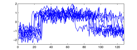
(a) Sample of time series

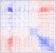
(b) Sample covariance

Figure 1: Ten samples of the Cylinder class from the CBF data set (Saito, 1994) and its sample covariance. Each time series has 128 data points. Higher absolute values in the matrix are presented using darker colors.

4.2 Moore-Penrose pseudoinverse and covariance shrinkage

Could it be that non-diagonal Mahalanobis distance measures could be superior or at least competitive with the diagonal Mahalanobis distance? It is tempting to use banded matrices, but the restriction of a positive definite matrix to a band may fail to be positive definite. Block-diagonal matrices (Matton et al, 2010) can preserve positive definiteness, but learning which blocks to use in the context of time series might be difficult. Instead, we propose two approaches: one is based on the widely used Moore-Penrose pseudoinverse, and the other is covariance shrinkage. See Figure 2 for the three different covariance estimates of the same class: sample covariance, shrinked covariance and diagonal covariance.

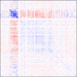
(a) Sample covariance

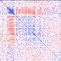
(b) Shrinked covariance

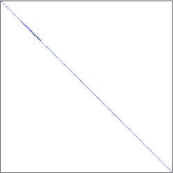
(c) Diagonal covariance

Figure 2: The covariance estimates of the Funnel class in the CBF data set. Large absolute values are in darker colors. Both the shrinked and diagonal covariances are positive definite whereas the sample covariance matrix is singular.

The approach based on the pseudoinverse is based on the singular value decomposition (SVD). We write the SVD as $C=U\Sigma V^{\top}$ where $\Sigma$ is a diagonal matrix with eigenvalues $\gamma_{1},\gamma_{2},\ldots$ and $U$ and $V$ are orthogonal matrices. The Moore-Penrose pseudoinverse is given by $V\Sigma^{+}U^{\top}$ where $\Sigma^{+}$ is the diagonal matrix made of the eigenvalues $1/\gamma_{1},1/\gamma_{2},\ldots$ with the convention that $1/0=0$. The pseudo-determinant is the product of the non-zero eigenvalues of $\Sigma$. We set $M$ equal to the pseudoinverse of the covariance matrix — normalized so that it has a pseudo-determinant of one. This solution is equivalent to projecting the time series data on the subspace corresponding to the non-zero eigenvalues of $\Sigma$. That is, the matrix $M$ is singular. Since the matrix $M$ is still a positive semi-definite matrix, the square root of the generalized ellipsoid distance measure remains a pseudometric: it is symmetric, non-negative and it satisfies the triangle inequality. But it is no longer a metric since it is possible to find distinct $\mathbf{x},\mathbf{y}$ such that $D_{M}(\mathbf{x},\mathbf{y})=0$.

Covariance shrinkage is an estimation method for problems with small number of instances and large number of attributes (Stein, 1956). It has better theoretical and practical properties for such data sets as the estimated covariance matrix is guaranteed to be non-singular. The covariance matrix $C$ is positive semi-definite but can be singular. To prevent $C$ from being singular, we replace it with an estimation of the form

$$C^{\star}=\lambda T+(1-\lambda)C$$

for some suitably chosen target matrix $T$: if $T$ is a positive definite matrix and $\lambda\in(0,1]$, we have that $\lambda T+(1-\lambda)C$ must be positive definite. Moreover, the smallest eigenvalue of $\lambda T+(1-\lambda)C$ must be at least as large as $\lambda$ times the smallest eigenvalue of $T$. We have used the target recommended by Schäfer and Strimmer (2005) which is the diagonal of the unrestricted covariance estimate, $T=\mathrm{diag}(C)$. It is positive definite in our examples. For $\lambda$, we use the estimation proposed by Schäfer and Strimmer (2005) (see Appendix A for details). We then set $M^{-1}\propto C^{\star}$, normalizing so that $\det(M)=1$. Unlike the pseudoinverse approach, covariance shrinkage generates a generalized ellipsoid distance measure which is a metric.

4.3 Global and class-specific distance measures

Given a training data set of time series, we can learn a single Mahalanobis distance measure from all time series, irrespective of their class labels (henceforth global Mahalanobis distance measure). We have a single matrix $M$. In this case the 1-NN classification algorithm works as follow: given a candidate time series $\mathbf{x}$ we seek $\mathbf{y}$ from the training set such that $D_{M}(\mathbf{x},\mathbf{y})$ is minimal. We then classify $\mathbf{x}$ in the same class as $\mathbf{y}$.

Otherwise, we may learn one Mahalanobis distance measure per class of time series. In this class-specific approach, the covariance matrix is computed solely from the time series of one class. Hence, for each class, we get one distance measure: class $i$ gets distance measure $D_{M_{i}}$. We have one matrix ($M_{i}$) per class ($i$). Given $\mathbf{y}$ from the training set, let $c(\mathbf{y})$ be the class of $\mathbf{y}$. Given a candidate time series $\mathbf{x}$, we classify it by finding $\mathbf{y}$ such that its distance to $\mathbf{x}$, $D_{M_{c(\mathbf{y})}}(\mathbf{x},\mathbf{y})$, is minimal. Hence, we not only compare the candidate time series $\mathbf{x}$ with time series from different classes, but we also use different distance measures.

Thus, finally, we consider six types of Mahalanobis distance measures for 1-NN classification: two localities (global or class-specific) and three estimators (pseudoinverse, shrinkage, or diagonal).

5 Experiments

The main goal of our experiments is to evaluate Mahalanobis distance measures and the class-specific approach on time series. More specifically, we ask the following questions.

• Of all the possible applications of the Mahalanobis distance measures (pseudoinverses, shrinkage or diagonal; class-specific or global), which one offers the best 1-NN classification accuracy? (§ 5.2)

• How do Mahalanobis distance measures compare with state-of-the-art alternatives such as DTW or LMNN? (§ 5.3)

• One of the simplest and most common distance measures, the Euclidean distance, is sometimes difficult to surpass for 1-NN classification of time series. To assess this effect, we ask how the relative accuracy of the Mahalanobis distance measure changes as we increase the number of instances per class in the training set. (§ 5.4)

We begin all tests with a training data set comprising several classes of time series. When applicable, distance measures are learned from this data set. We then attempt to classify some test data using 1-NN. We define the classification error to be the percentage of misclassified instances whereas the accuracy is the percentage of properly classified instances.

The code for the experiments is available online (Prekopcsák, 2011) with instructions on how the results can be reproduced. For LMNN, we use the source code provided by Weinberger and Saul (2008) for the experiments with default parameters. For the DTW, we find the best monotonic matching $\Gamma$ minimizing ${\sum_{(i,j)\in\Gamma}|x_{i}-y_{j}|^{2}}$. The computational cost of the DTW is sometimes a challenge (Salvador and Chan, 2007). To alleviate this problem, several strategies have been proposed including lower bounds and R^⋆-tree indexes (Ratanamahatana and Keogh, 2005; Lemire, 2009; Ouyang and Zhang, 2010). For our purposes, we use a quadratic-time dynamic programming algorithm. In contrast, the Euclidean and diagonal Mahalanobis distance measures only require linear time. We ran the experiments on a MacBook Pro laptop with a 2.3 GHz Intel Core i5 processor and 8 GB of RAM. All code ran on Matlab R2011a.

5.1 Data sets

We use the UCR time series classification benchmark (Keogh et al, 2006) for our experiments as it includes diverse time series data sets from many domains. It has predefined training-test splits for the experiments (see Table 1), so the results can be compared across different papers. Most of the data sets are z-normalized: that is, the time series have zero mean and a variance of one. We removed the two data that are not z-normalized by default (Beef and Coffee). Indeed, z-normalization improves substantially the classification accuracy — irrespective of the chosen distance measure. Thus, for fair results, we should z-normalize them, but this may create confusion with previously reported numbers. We also removed the Wafer data set as all distance measures classify it nearly perfectly. The remaining 17 data sets were used for the comparison of different methods.

Table 1: Number of classes, number of instances in both the training and testing sets, and the length of the time series in each data set.

Data set	classes	training set	testing set	length ($n$)
50 words	50	450	455	270
Adiac	37	390	391	176
CBF	3	30	900	128
ECG	2	100	100	96
Fish	7	175	175	463
Face (all)	14	560	1 690	131
Face (four)	4	24	88	350
Gun-Point	2	50	150	150
Lighting-2	2	60	61	637
Lighting-7	7	70	73	319
OSU Leaf	6	200	242	427
OliveOil	4	30	30	570
Swedish Leaf	15	500	625	128
Trace	4	100	100	275
Two Patterns	4	1 000	4 000	128
Synthetic Control	6	300	300	60
Yoga	2	300	3 000	426

5.2 Best Mahalanobis distance measure for 1-NN accuracy

We compare the various Mahalanobis distance measures in Table 2. We have left out the Moore-Penrose pseudoinverse, because its error rates were twice as high on average compared to the other variants. What is immediately apparent is that the class-specific measures give better classification results.

The diagonal Mahalanobis has a smaller classification error and is considerably faster (3.7 min compared to 5.5 min on the whole data set), but the shrinkage estimate yields significantly better results for several data sets (e.g. Adiac and Fish). Thus, out of the six variations, we recommend the class-specific covariance-shrinkage estimate and the class-specific diagonal Mahalanobis distance measures.

Table 2: Classification error for the various Mahalanobis distance measures.

Data set	Shrinkage		Diagonal
	global	class-specific	global	class-specific
50 words	0.34	0.71	0.34	0.32
Adiac	0.33	0.30	0.37	0.36
CBF	0.34	0.06	0.16	0.05
ECG	0.12	0.10	0.10	0.08
Fish	0.31	0.15	0.19	0.18
Face (all)	0.32	0.27	0.32	0.25
Face (four)	0.27	0.16	0.16	0.17
Gun-Point	0.12	0.14	0.10	0.11
Lighting-2	0.31	0.30	0.25	0.25
Lighting-7	0.55	0.32	0.36	0.23
OSU Leaf	0.68	0.69	0.46	0.46
OliveOil	0.17	0.20	0.17	0.13
Swedish Leaf	0.24	0.15	0.21	0.18
Trace	0.40	0.12	0.21	0.07
Two Patterns	0.12	0.12	0.12	0.12
Synthetic Control	0.23	0.08	0.13	0.09
Yoga	0.26	0.22	0.17	0.17
# of best errors	0	5	5	10

5.3 Comparing competitive distance measures

How do the class-specific Mahalanobis distance measures behave in comparison with competitive distance measures? Computationally, the diagonal Mahalanobis is inexpensive compared to schemes such as the DTW or LMNN. Regarding the 1-NN classification error rate, we give the results in Table 3. As expected (Ding et al, 2008), no distance measure is better on all data sets. However, because the diagonal Mahalanobis distance measure is closely related to the Euclidean distance, we compare their classification accuracy. In two data sets, the Euclidean distance outperformed the class-specific Mahalanobis distance measures and only by small differences (0.09 versus 0.10–0.12). Meanwhile, the class-specific diagonal Mahalanobis distance measures outperformed the Euclidean distance 12 times, and sometimes by large margins (0.07 versus 0.24 and 0.05 versus 0.15). The LMNN is also competitive: its classification error is sometimes half that of the Euclidean distance.

The DTW has the lowest error rates and provides best results for half of the data sets, but it is much slower than Mahalanobis distance measures. It takes 3.7 min (diagonal) and 5.5 min (covariance shrinkage) to compute the Mahalanobis results on the whole data set. As expected, the diagonal Mahalanobis is nearly as fast as the Euclidean distance (3.5 min). The LMNN takes 18 min and the DTW runs for 18 hours. The DTW is at least two orders of magnitude slower than the diagonal Mahalanobis on all 17 data sets.

Table 3: Classification errors for some competitive schemes. For all distance measures, we use 1-NN classification. For the 50 words data set, the LMNN computation fails because it has a class with only one instance. For this table, we used the class-specific Mahalanobis distance measure.

Data set	Euclidean	DTW	Mahalanobis		LMNN
			shrink.	diag.
50 words	0.37	0.31	0.71	0.32	–
Adiac	0.39	0.40	0.30	0.36	0.23
CBF	0.15	0.00	0.06	0.05	0.15
ECG	0.12	0.23	0.10	0.08	0.10
Fish	0.22	0.17	0.15	0.18	0.13
Face (all)	0.29	0.19	0.27	0.25	0.16
Face (four)	0.22	0.17	0.16	0.17	0.16
Gun-Point	0.09	0.09	0.14	0.11	0.05
Lighting-2	0.25	0.13	0.30	0.25	0.41
Lighting-7	0.42	0.27	0.32	0.23	0.51
OSU Leaf	0.48	0.41	0.69	0.46	0.57
OliveOil	0.13	0.13	0.20	0.13	0.13
Swedish Leaf	0.21	0.21	0.15	0.18	0.21
Trace	0.24	0.00	0.12	0.07	0.20
Two Patterns	0.09	0.00	0.12	0.12	0.05
Synthetic Control	0.12	0.01	0.08	0.09	0.03
Yoga	0.17	0.16	0.22	0.17	0.18
# of best errors	1	9	2	3	6

5.4 Effect of the number of instances per class

Whereas Table 3 shows that the Mahalanobis distance measures are far superior to the Euclidean distance on some data sets, this result is linked to the number of instances per class. For example, on the Wafer data set (which we removed), there are many instances per class (500), and correspondingly, all distance measures give a negligible classification error.

Thus, we considered three different synthetic time-series data-set generators with varying numbers of instances per class:

• Cylinder-Bell-Funnel (CBF) (Saito, 1994),

• Control Charts (CC) (Pham and Chan, 1998) and

• Waveform (Breiman, 1998).

The CC data is made of 6 classes containing time series made of 60 data points; CBF is made of 3 classes and its time series have 128 data points; Waveform has 3 classes and its time series are made of 21 data points. All time series are z-normalized (zero mean and a variance of one). The CBF data set from Tables 2 and 3 was generated from the same data-set model, except that we vary the number of time series (see Appendix B).

Test sets have 1 000 instances per class whereas training sets have between 10 to 1 000 instances. We repeated each test ten times, with different training sets. Fig. 3 shows that whereas the class-specific diagonal Mahalanobis distance measures are superior to the Euclidean distance when there are few instances, this benefit is less significant as the number of instances increases. Indeed, the classification accuracy of the Euclidean distance grows closer to perfection and it becomes more difficult for alternatives to be far superior.

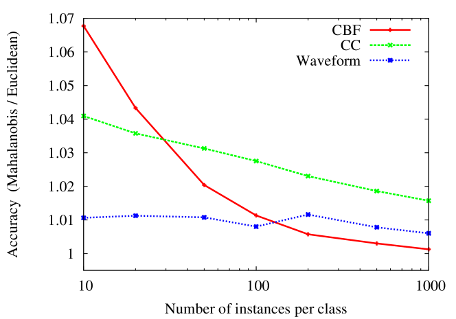
Figure 3: Ratios of the 1-NN classification accuracies using the class-specific diagonal Mahalanobis and Euclidean distance measures

6 Conclusion

The Mahalanobis distance measures have received little attention for time series classification and we are not surprised given their poor performance as a 1-NN classifier when used in a straight-forward manner. However, by learning one Mahalanobis distance measure per class we get a competitive classifier when using either covariance shrinkage or a diagonal approach. Moreover, the diagonal Mahalanobis distance measure is particularly appealing computationally: we only need to compute the variances of the components. Meanwhile, we get good results with the LMNN on time series data, though it is more expensive. The DTW is superior, but it is one to two orders of magnitude slower.

Appendix A Choice of the parameter $\lambda$ in covariance shrinkage

Covariance shrinkage (see § 4) requires the choice of a parameter $\lambda\in(0,1]$, which should be sufficiently large so that $\lambda T+(1-\lambda)C$ is numerically invertible. We choose $T$ to be the diagonal of the covariance matrix $C$ ($T=\mathrm{diag}(C)$).

To give the formula for $\lambda$ proposed by Schäfer and Strimmer (2005), we need to introduce some technical notation. Given a family of time series $\mathbf{x}^{(1)},\mathbf{x}^{(2)},\ldots,\mathbf{x}^{(N)}$, we write the average of the $i^{\mathrm{th}}$ component as $\bar{z}_{i}=\sum_{k=1}^{N}\mathbf{x}^{(k)}_{i}$. We write

$$w_{kij}=(\mathbf{x}^{(k)}_{i}-\bar{z}_{i})(\mathbf{x}^{(k)}_{j}-\bar{z}_{j})$$

and $w_{ij}=\frac{1}{N}\sum_{k=1}^{N}w_{kij}$. Moreover, we write

$$\widehat{\mathrm{Var}}(c_{ij})=\frac{N}{(N-1)^{3}}\sum_{k=1}^{N}(w_{kij}-w_{ij})^{2}.$$

Finally, we have

$$\lambda^{\star}=\frac{\sum_{i\neq j}\widehat{\mathrm{Var}}(c_{ij})}{\sum_{i\neq j}c_{ij}^{2}}$$

where $c_{ij}$ are the components of the (sample) covariance matrix $C$ (see § 3). We set $\lambda$ to $\lambda^{\star}$ when $\lambda^{\star}\leq 1$. Otherwise, we set $\lambda=1$.

We experimented informally with different values of $\lambda$ (using the data sets from from § 5) and found that the choice preconised by Schäfer and Strimmer (2005) was reasonable. That is, we did not find a case where a different value of $\lambda$ gave much better classification accuracy.

Appendix B The Cylinder-Bell-Funnel (CBF) data model

Consider the original CBF data model (Saito, 1994). We can use it to generate time series of three possible classes. In the case where we have only 10 time series for each class in the training data set and a large number of time series in the test set (1000), we find that, over ten tests, the average 1-NN classification error rate is 0.20 ($\sigma=0.04$) for the Euclidean distance and 0.15 ($\sigma=0.03$) for the diagonal Mahalanobis distance measure. These results are difficult to reconcile with Table 3 where we used a similar number of CBF time series provided by Keogh et al (2006) and where we report error rates of 0.15 and 0.05. Indeed, the difference in error rate for the diagonal Mahalanobis distance measure exceeds 3 standard deviations.

After inspection, we found that the CBF data model used by Keogh et al (2006) differs from the original presentation by Saito (1994). They both generate time series using random functions of the form: $c(i)=(6+\eta)\cdot\chi_{[a,b]}(i)+\varepsilon(i)$, $b(i)=(6+\eta)\cdot\chi_{[a,b]}(i)\cdot(i-a)/(b-a)+\varepsilon(i)$ and $f(i)=(6+\eta)\cdot\chi_{[a,b]}(i)\cdot(b-i)/(b-a)+\varepsilon(i)$ where $i=1,\ldots,128$ and $\chi_{[a,b]}$ is the characteristic function. They both use standard normal variates for $\eta$ and $\varepsilon(i)$, and uniformly distributed $a$ integer values in $[16,32]$. However, whereas Saito (1994) states that $b-a$ obeys an integer-valued uniform distribution on $[32,96]$, we found that Keogh et al (2006) generated their CBF data so that $b-32$ is an integer-valued uniform distribution on $[32,96]$.

If we adopt the Keogh et al (2006) variation, the classification error rates go down: 0.16 ($\sigma=0.03$) for the Euclidean distance and 0.10 ($\sigma=0.04$) for the diagonal Mahalanobis distance measure. These results are nearly within a standard deviation of the results presented in Table 3 for CBF.