Coherent Radiation by a Spherical Medium of Resonant Atoms

Abstract

Radiation by the atoms of a resonant medium is a cooperative process in which the medium participates as a whole. In two previous papers PG00 ; GP00 , we treated this problem for the case of a medium having slab geometry, which, under plane wave excitation, supports coherent waves that propagate in one dimension. We extend the treatment here to the three-dimensional problem, focusing principally on the case of spherical geometry. By regarding the radiation field as a superposition of electric and magnetic multipole fields of different orders, we express it in terms of suitably defined scalar fields. The latter fields possess a sequence of exponentially decaying eigenmodes corresponding to each multipole order. We consider several examples of spherically symmetric initial excitations of a sphere. Small uniformly excited spheres, we find, tend to radiate superradiantly, while the radiation from a large sphere with an initially excited inner core exhibits temporal oscillations that result from the participation of a large number of coherently excited amplitudes in different modes. The frequency spectrum of the emitted radiation possesses a rich structure, including a frequency gap for large spheres and sharply defined and closely spaced peaks caused by the small frequency shifts and even smaller decay rates characteristic of the majority of eigenmodes.

I INTRODUCTION

A quantum of light emitted within a finite medium made of identical atoms cannot easily escape. It may suffer a large and undeterminable number of coherent absorption and reemission processes before reaching the boundary of the medium, and even there is subject to the hazard of internal reflection. The emission of a quantum by a single atom within such a medium, in other words, is inevitably a process in which the entire medium partakes coherently. When more than one atom is excited initially, they tend to radiate cooperatively and that sort of coherent emission process is often referred to as superradiance Dicke54 ; AC70 ; BL76 ; GH76 ; GH82 ; PG85 . The time dependence of the energy emitted by the medium in all these cases may differ considerably from the exponential decay characteristic of the isolated atom, and its frequency spectrum may differ substantially from the familiar Lorentzian form. In the present paper we address ourselves to the analysis of these effects for the important case in which the medium is spherical in shape and all the inhomogeneities that destroy coherence are assumed negligible.

The medium we envisage consists of identical atoms, all with the same electric dipole resonance at a (renormalized) frequency $\omega_{0}$. Since they are never more than weakly excited, the atoms may be replaced, in effect, by harmonic oscillators of the same frequency. We assume them to be distributed densely enough that many are present in each cubic wavelength $(2\pi c/\omega_{0})^{3}$, and smoothly enough to permit treating the medium as a continuum. We have called this idealized model of a resonant and isotropically polarizable medium polarium, and have discussed a number of its behaviors in two previous papers, I PG00 and II GP00 . In those papers, we discussed the emission and propagation of radiation in the essentially one-dimensional context of parallel slab geometry. The plane waves that are radiated, we showed, can be regarded as a superposition of contributions from a sequence of mutually orthogonal polarization modes that decay exponentially and have easily calculated properties.

The modal decomposition of the polarization in the one-dimensional medium revealed in I a complex structure for the time dependence of its decay. An oscillatory exchange of energy takes place, in effect, between the coherently coupled radiation and polarization fields. The radiated spectrum consequently exhibits an elaborate structure of narrow peaks and dips corresponding to mutually interefering resonant amplitudes contributed by the various modes. A gap is also present in the spectrum, corresponding to a band of frequencies in which the implicit dispersion law of the medium suppresses propagation. Not surprisingly, these features are also found to play an important role in the discussion of reflection and transmission of an externally incident plane wave by a slab shaped medium that we undertook in II. By changing the angle of incidence and the polarization direction of the incident wave, we could tune and alter the spectral dependences of the reflection and transmission coefficients in predictable ways.

One of our early tasks in analyzing the problem in spherical geometry will be to find the appropriate set of exponentially decaying polarization modes. These must obey conditions that assure the transverse character of the radiated fields. In I, transversality was easily secured by dealing only with fields uniform over planes perpendicular to the axis of propagation. In II, where plane waves could be obliquely incident upon the slab shaped medium, a more careful treatment of the separated Cartesian field components was required since induced surface charges and currents complicate the boundary conditions.

For the spherical geometry we find it particularly convenient to introduce two familiar angular momentum projection operators to separate the full vector field problem into its electric and magnetic multipole parts. Each of these parts can be further resolved into a succession of spherical harmonic components. The magnetic multipole fields separated in this way automatically obey the required transversality conditions. The electric multipole fields, on the other hand, still require some consideration of surface charges and currents in order to secure transversality. The most convenient feature of the angular momentum decomposition is that it involves only scalar functions which are in effect the radial components of the electric and magnetic fields. We may express these components in terms of mode functions that decay exponentially with time in each spherical harmonic order.

We begin in Sec. II with the elementary example of radiation from a small uniformly excited sphere. This problem, which can be solved directly without the use of angular momentum operators, provides physical insights into the coherent radiation problem, which are useful in treating the problem of larger spheres. In Sec. III, we present the equations of motion for the radiation field and polarization. The complications of maintaining a transverse displacement field everywhere are handled here by means of the two angular momentum projection operators. Their use leads to equations of motion for the electric and magnetic fields and for their polarization sources. The magnetic multipole radiation, which is analytically simpler to treat, is discussed in Sec. IV, while a full treatment of the electric multipole radiation is begun in Sec. V. The magnetic multipole radiation field obeys simple outgoing-wave boundary conditions in each angular momentum order. We derive the eigenvalue equation that results from these boundary conditions and briefly discuss certain important properties of the exponentially decaying eigenmodes. The electric multipole radiation problem requires somewhat more involved outgoing-wave boundary conditions that can be most simply treated by considering the differential equations obeyed by the electric and displacement fields inside and outside the medium. When the medium excitation is restricted to initial polarizations that are oriented along a fixed direction and have a radially symmetric but otherwise arbitrary amplitude, the spherical medium, regardless of its radius, radiates as a pure electric dipole, as we show in Sec. V. In the same section, the associated electric-dipole eigenvalue problem is developed in the more general context of electric multipoles of arbitrary order, and the eigenvalue equation is analytically solved for the eigenvalues in several important limiting cases. In Sec. VI, we establish the orthogonality of electric multipole modes of an arbitrary order. In Sec. VII we discuss the temporal and spectral characteristics of the electric dipole radiation from an interesting example of a spherical system, one in which a uniformly excited spherical core is surrounded by an initially unexcited spherical shell. Finally, in Sec. VIII, some concluding remarks about the problem of coherent transport of resonant excitations treated here are presented.

II AN ELEMENTARY EXAMPLE: RADIATION FROM A SMALL UNIFORMLY EXCITED SPHERE

It will be useful to begin our analysis by discussing the radiation by a spherical medium of radius $R$ much smaller than the reduced wavelength $1/k_{0}=c/\omega_{0}$, i.e., $\beta\equiv k_{0}R<<1$. The problem is simple enough to afford elementary access. It will furnish a valuable example for later reference.

The atoms of the medium we call polarium are assumed to be distributed with a uniform density $n_{0}$. The transition matrix elements of their electric dipole moment vectors $\vec{\mu}$ are assumed to be randomly oriented so that the medium is isotropic, and its induced electric polarization is always parallel to the inducing field. Then, as we have shown in deriving Eq. (9) of I, the positive frequency part of the polarization field $\vec{P}^{(+)}(\vec{r},t)$ for such a medium is driven by the positive frequency part of the electric field $\vec{E}^{(+)}(\vec{r},t)$ through the relation

$$\left({\partial\over\partial t}+i\omega_{0}\right)\vec{P}^{(+)}(\vec{r},t)={in_{0}|\vec{\mu}|^{2}\over 3\hbar}\vec{E}^{(+)}(\vec{r},t).$$ (1)

In the absence of the electric field, the polarization varies in time at any point as $\exp(-i\omega_{0}t)$.

By expressing $\vec{E}^{(+)}$ and $\vec{P}^{(+)}$ in terms of their slowly-varying envelopes $\vec{\cal E}$ and $\vec{\cal P}$:

$$\vec{E}^{(+)}(\vec{r},t)=\vec{\cal E}(\vec{r},t)e^{-i\omega_{0}t},\ \ \vec{P}^{(+)}(\vec{r},t)=\vec{\cal P}(\vec{r},t)e^{-i\omega_{0}t},$$ (2)

we may rewrite Eq. (1) as

$${\partial\over\partial t}{\cal P}(\vec{r},t)={in_{0}|\vec{\mu}|^{2}\over 3\hbar}{\cal E}(\vec{r},t).$$ (3)

We shall assume that the polarization is spatially uniform and given by $\hat{z}P(t)\exp(-i\omega_{0}t)$, where $\hat{z}$ is a unit vector along the $z-$axis. In that case, the fields generated by the uniform polarization, although rapidly oscillating in time, have the familiar electrostatic spatial dependence within the near field zone. Thus the electric field within the sphere is uniform and parallel to the polarization. The magnetic field within the medium is of relative order $k_{0}R<<1$, and is thus negligible in this, the long wavelength limit.

Such a uniformly polarized small sphere decays superradiantly, as we shall see presently. If $\lambda_{0}$ is the exponential decay constant for this mode, then the electric field within the medium, which we denote by $\vec{E}^{<}$, and the polarization $P_{0}\exp(-\lambda_{0}t)$ are formally related, according to Eq. (3), by

$$\vec{E}^{<}=\hat{z}{3i\hbar\lambda\over n_{0}|\vec{\mu}|^{2}}P_{0}e^{-\lambda_{0}t}e^{-i\omega_{0}t}.$$ (4)

Outside the medium, the electric field $\vec{E}^{>}$ is that of a point dipole $\vec{p}_{0}$, equal in value to the dipole moment of the sphere,

$$\vec{p}_{0}=\hat{z}P_{0}{4\pi\over 3}R^{3},$$ (5)

and located at its center. In the near field zone, the electric field thus assumes the familiar elecrostatic spatial dependence

$$\vec{E}^{>}={3(\vec{p}_{0}\cdot\hat{r})\hat{r}-\vec{p}_{0}\over 4\pi r^{3}}e^{-\lambda_{0}t}e^{-i\omega_{0}t}.$$ (6)

The eigenvalue $\lambda_{0}$ is determined by requiring that in the long-wavelength limit the electric field in the interior of a uniformly polarized small sphere be minus a third of its polarization, $\vec{E}^{<}=-(1/3)\vec{P}$. In view of Eq. (4), this requirement yields the following expression for $\lambda_{0}$:

$$\lambda_{0}=i{n_{0}|\vec{\mu}|^{2}\over 9\hbar}.$$ (7)

Because the eigenvalue (7) is purely imaginary, it represents merely a frequency shift for the field and polarization. The sphere does not radiate in the limit $\beta\to 0$. For small but finite $\beta$, the sphere does, in fact, radiate. To calculate the decay rate ${\rm Re}\lambda_{0}$, we resort to an analysis based on the rate at which a uniformly polarized sphere, with its polarization oscillating at frequency $\omega_{0}$, radiates energy. A small sphere of this kind radiates as an oscillating point dipole Jackson1 at the time-averaged rate footnote1

$$W={c|\vec{p}_{0}|^{2}k_{0}^{4}\over 3\pi}.$$ (8)

Equivalently, the rate at which energy is lost from the dipoles of the spherical medium must be equal to the rate at which work is done by them on the field. The rate of work done by the $i$th dipole of dipole moment $\vec{p}_{i}$, when averaged over the fundamental period of oscillation, is just $-2{\rm Re}\,\dot{\vec{p}_{i}^{*}}\cdot\vec{E}$, where $\dot{\vec{p}_{i}}$ is the time derivative of the dipole moment. Therefore the rate at which work is done by the sphere is $-2{\rm Re}\,\dot{\vec{P}^{*}}\cdot\vec{E}(4\pi R^{3}/3)$. Since the polarization and field both oscillate at a frequency close to $\omega_{0}$, the preceding expression is essentially the same as

$$W={8\pi R^{3}\over 3}\omega_{0}{\rm Im}\,\vec{P}^{*}\cdot\vec{E}.$$ (9)

When the relation (1) between the field and polarization is used to eliminate $\vec{E}$ from Eq. (9), the resulting expression for $W$ is

$$W={8\pi R^{3}\omega_{0}}{{\rm Re}\,\lambda_{0}\over(n_{0}|\vec{\mu}|^{2}/\hbar)}|\vec{P}|^{2}.$$ (10)

An explicit expression for the decay rate ${\rm Re}\,\lambda_{0}$ is now obtained by equating Eqs. (8)) and (10) and using Eq. (5),

$${\rm Re}\,\lambda_{0}={2\over 27}{n_{0}|\vec{\mu}|^{2}\over\hbar}\beta^{3}.$$ (11)

The rate (11) at which a small uniformly polarized sphere decays radiatively may be expressed as the product of the number of atoms, $N=n_{0}(4\pi R^{3}/3)$, and the Wigner-Weisskopf intrinsic decay rate of each atom, $\tau^{-1}=|\vec{\mu}|^{2}k_{0}^{3}/(18\pi\hbar)$:

$${\rm Re}\,\lambda_{0}={N}\tau^{-1}.$$ (12)

Each dipole in an assembly of $N$ identically prepared and coherently coupled atomic dipoles emits radiation at a rate that is $N$ times the rate with which it would spontaneously radiate when isolated from the others. Such enhanced decay rates are characteristic of superradiant emission, a process that is often considered in the context of much stronger excitation of the radiating medium, e.g., when all of the atoms are fully excited in the initial state. In these more general examples the emission process can only be described adequately by means of nonlinear equations. The present problem, by contrast, is considerably simpler due to its linearity in the fields and polarization. Because of the coherent initial preparation of the atomic dipoles, the essential coherence always remains present in the emission process.

It is worth recalling here that Hartmann and collaborators FHM72 ; FH74 have made an important criticism of Dicke’s elementary theory of superradiance in many-atom systems. They have pointed out that the electric dipole moments induced in different atoms will interact strongly via the familiar dipole-dipole interactions and lead to spatially dependent shifts of atomic energy levels. These differing level shifts can bring about relative dephasing of different parts of the oscillating polarization distribution and thus some breakdown of the cooperative character of superradiant emission. We see no evidence of this suppression in the radiative rate given by Eq. (12). Indeed, the way in which we have treated the interaction of each atom with the field implicitly includes the effects of all dipole-dipole interactions. Their total effect does not inhibit superradiance, at least for the linear problem of radiation from a small uniformly polarized sphere.

III FORMULATION OF THE GENERAL PROBLEM

We now turn to the general problem of radiation by an arbitrary excitation of a spherical medium of arbitrary radius. The resonant interaction of the polarium medium with the electromagnetic field is described by Eq. (1) and the Maxwell wave equation

$$-\vec{\nabla}\times(\vec{\nabla}\times\vec{E}^{(+)})-{1\over c^{2}}{\partial^{2}\over\partial t^{2}}\vec{E}^{(+)}={1\over c^{2}}{\partial^{2}\over\partial t^{2}}\vec{P}^{(+)}.$$ (13)

Because of the identity

$$-\vec{\nabla}\times(\vec{\nabla}\times\vec{E}^{(+)})=\nabla^{2}\vec{E}^{(+)}-\vec{\nabla}(\vec{\nabla}\cdot\vec{E}^{(+)}),$$ (14)

Eq. (14) contains an explicit gradient term, $\vec{\nabla}(\vec{\nabla}\cdot\vec{E}^{(+)})$, which enforces the transversality of the total displacement field, $\vec{D}=\vec{E}+\vec{P}$. We shall see later that this term greatly influences the character of the radiation and most particularly when the spheres are small compared to the wavelength of radiation.

The spherical geometry of the radiation problem is best approached by decomposing the radiation field into its electric multipole (EM) and magnetic multipole (MM) components, and introducing appropriate scalar functions to describe them. A simple way to exhibit this decomposition without introducing the full panoply of vector spherical harmonics is to use two operators Jackson1 ; PG85 that are simply related to the quantum-mechanical angular-momentum operator, $\vec{L}=-i\vec{r}\times\vec{\nabla}$. Let us consider the action of the operators $\vec{L}\cdot$ and $\vec{L}\cdot\vec{\nabla}\times$ on Eqs. (1) and (13). Because both these operators annihilate the gradient term inside the double curl when identity (14) is used and because they commute with the Laplacian, Eq. (13) simplifies to an inhomogeneous scalar wave equation of the general form

$$\left(\nabla^{2}-{1\over c^{2}}{\partial^{2}\over\partial t^{2}}\right)\eta(\vec{r},t)={1\over c^{2}}{\partial^{2}\over\partial t^{2}}\phi(\vec{r},t),$$ (15)

where the symbols, $\phi$ and $\eta$, denote the functions

$$\phi=\vec{L}\cdot\vec{P}^{(+)}\ {\rm and}\ \eta=\vec{L}\cdot\vec{E}^{(+)})$$ (16)

or alternatively

$$\phi=\vec{L}\cdot\vec{\nabla}\times\vec{P}^{(+)}\ {\rm and}\ \eta=\vec{L}\cdot\vec{\nabla}\times\vec{E}^{(+)}).$$ (17)

That $\vec{L}\cdot\vec{E}^{(+)}$ and $\vec{L}\cdot\vec{\nabla}\times\vec{E}^{(+)}$ describe the radial components of the magnetic and electric fields and thus the MM and EM fields, respectively, is immediately evident when the vector triple products are rearranged, and the Faraday and Maxwell-Ampère laws are introduced as follows:

$$\vec{L}\cdot\vec{E}^{(+)}\sim (\vec{r}\times\vec{\nabla})\cdot\vec{E}^{(+)}=\vec{r}\cdot(\vec{\nabla}\times\vec{E}^{(+)})$$

$$\sim\vec{r}\cdot{\partial\over\partial t}\vec{B}^{(+)}\sim\vec{r}\cdot\vec{B}^{(+)}$$

$$\vec{L}\cdot\vec{\nabla}\times\vec{E}^{(+)}\sim \vec{L}\cdot\vec{B}^{(+)}\sim\vec{r}\cdot(\vec{\nabla}\times\vec{B}^{(+)})$$

$$\sim\vec{r}\cdot{\partial\over\partial t}\vec{E}^{(+)}\sim\vec{r}\cdot\vec{E}^{(+)}.$$ (18)

The final step in each of the two relations in Eq. (III) has employed the assumption of quasi-monochromaticity, which permits replacing time differentiations of the positive-frequency parts of the electromagnetic field by the multiplicative factor $-i\omega_{0}$. The validity of this assumption is assured by the resonant character of the radiative interactions in the medium.

By contrast with Eq. (13), Eq. (1) is formally unchanged when the spatial operator $\vec{L}\cdot$ is applied,

$$\left({\partial\over\partial t}+i\omega_{0}\right)\phi(\vec{r},t)={in_{0}|\vec{\mu}|^{2}\over 3\hbar}\eta(\vec{r},t),$$ (19)

where $\phi$ and $\eta$ are given by Eq. (16). Under the $\vec{L}\cdot\vec{\nabla}\times$ operation, however, the sharp drop-off at the surface of the otherwise uniform medium density contributes to the right-hand side of Eq. (19) a surface singularity Jackson2 , which is generated by oscillating surface charges. Such surface polarization charges and currents must be present for EM radiation for which both the electric field and polarization have nonvanishing radial components. A self-consistent approach that treats these surface singularities correctly but implicitly is based on matching on the surface the appropriate components of the electromagnetic field inside the medium to those outside.

The $\vec{L}\cdot$ operation commutes with the density which has only a radial step-function form. Eq. (19) is thus valid both in the interior and on the surface of the medium. That is to say, for MM radiation, the electric field and polarization are both purely transverse, and no surface charges are present.

For the problem of radiation from an initially excited medium with no externally incident fields, Eq. (III) admits the familiar sort of retarded integral solution for $\eta$:

$$\eta(\vec{r},t)= - {1\over c^{2}}\int{\partial^{2}\over\partial t^{\prime 2}}\phi(\vec{r}^{\,\prime},t^{\prime}){\delta\left(t-t^{\prime}-{|\vec{r}-\vec{r}^{\,\prime}|\over c}\right)\over 4\pi|\vec{r}-\vec{r}^{\,\prime}|}d\vec{r}^{\,\prime}dt^{\prime}$$

$$= - {1\over c^{2}}\int{{\partial^{2}\over\partial t^{2}}\phi\left(\vec{r}^{\,\prime},t-{|\vec{r}-\vec{r}^{\,\prime}|\over c}\right)\over 4\pi|\vec{r}-\vec{r}^{\,\prime}|}d\vec{r}^{\,\prime}.$$ (20)

By expressing $\eta$ and $\phi$ in terms of their slowly-varying envelopes ${\cal E}$ and ${\cal P}$:

$$\eta(\vec{r},t)={\cal E}(\vec{r},t)e^{-i\omega_{0}t},\ \ \phi(\vec{r},t)={\cal P}(\vec{r},t)e^{-i\omega_{0}t},$$ (21)

and dropping the time derivatives of ${\cal P}$, which may be assumed small, we may reduce Eq. (III) to the form

$${\cal E}(\vec{r},t)=k_{0}^{2}\int{\cal P}\left(\vec{r}^{\,\prime},t-{|\vec{r}-\vec{r}^{\,\prime}|\over c}\right){e^{ik_{0}|\vec{r}-\vec{r}^{\,\prime}|}\over 4\pi|\vec{r}-\vec{r}^{\,\prime}|}d\vec{r}^{\,\prime}.$$ (22)

Because Eq. (19) fails to include radiating surface currents, the description provided by Eqs. (19)) and (22) is not complete for EM radiation. But these equations do, however, describe properly MM radiation which has no surface sources for a spherical radiator.

IV MAGNETIC MULTIPOLE RADIATION AND THE ASSOCIATED EIGENVALUE PROBLEM

The use of the envelopes (21) in Eq. (19) leads to the equation of motion for the polarization multipoles,

$${\partial\over\partial t}{\cal P}(\vec{r},t)=i{|\vec{\mu}|^{2}\over 3\hbar}n_{0}{\cal E}(\vec{r},t).$$ (23)

By eliminating the field multipoles ${\cal E}$ between Eqs. (22) and (23), we secure the integral equation for the polarization multipole fields

$${\partial\over\partial t}{\cal P}(\vec{r},t)=i{|\vec{\mu}|^{2}n_{0}k_{0}^{2}\over 3\hbar}\int {e^{ik_{0}|\vec{r}-\vec{r}^{\,\prime}|}\over 4\pi|\vec{r}-\vec{r}^{\,\prime}|}$$

$$\times{\cal P}\left(\vec{r}^{\,\prime},t-{|\vec{r}-\vec{r}^{\,\prime}|\over c}\right)d\vec{r}^{\,\prime}.$$ (24)

The integrand on the right side of Eq. (IV) requires evaluating the envelope function ${\cal P}$ at the retarded time $t-|\vec{r}-\vec{r}^{\,\prime}|/c$, but if its temporal variation is sufficiently slow it remains accurate to neglect the retardation in ${\cal P}$ and write

$${\partial\over\partial t}{\cal P}(\vec{r},t)=i{|\vec{\mu}|^{2}n_{0}k_{0}^{2}\over 3\hbar}\int{e^{ik_{0}|\vec{r}-\vec{r}^{\,\prime}|}\over 4\pi|\vec{r}-\vec{r}^{\,\prime}|}{\cal P}\left(\vec{r}^{\,\prime},t\right)d\vec{r}^{\,\prime}.$$ (25)

The more important effects of retardation are still retained in the exponential function in the integrand. This approach, we have called the rapid-transit approximation in I, assumes only that the slowly varying amplitude ${\cal P}$ does not change appreciably during the passage time of a wave through the medium. The approximation is not essential to our treatment of the problem, but it greatly simplifies the analysis, and we shall therefore employ it in exploring the behavior of the system.

Let us consider an expansion of ${\cal P}(\vec{r},t)$ in spherical harmonics, defined according to the convention employed in Ref. Jackson2 ,

$${\cal P}(\vec{r},t)=\sum_{\ell,m}P_{\ell m}(r,t)Y_{\ell m}(\vec{\Omega}).$$ (26)

Substitution of this form into Eq. (25), followed by a use of the identity

$${e^{ik_{0}|\vec{r}-\vec{r}^{\,\prime}|}\over 4\pi|\vec{r}-\vec{r}^{\,\prime}|}=ik_{0}\sum_{\ell,m}j_{\ell}(k_{0}r^{<})h_{\ell}^{(1)}(k_{0}r^{>})Y_{\ell m}(\vec{\Omega})Y^{*}_{\ell m}(\vec{\Omega}^{\prime}),$$ (27)

and integration over the solid angles $\vec{\Omega}^{\prime}$ of the vector $\vec{r}^{\,\prime}$, together with a use of the orthonormality and linear independence of the various spherical harmonics yields the result

$${\partial\over\partial t}{\cal P}_{\ell m}(r,t)=- {n_{0}|\vec{\mu}|^{2}k_{0}^{3}\over 3\hbar}\int_{0}^{R}{\cal P}_{\ell m}(r^{\prime},t)$$

$$\times j_{\ell}(k_{0}r^{<})h_{\ell}^{(1)}(k_{0}r^{>})r^{\prime 2}dr^{\prime}.$$ (28)

Here $j_{\ell}$ and $h_{\ell}^{(1)}$ are spherical Bessel and Hankel functions of the first kind, and $r^{<}(r^{>})$ is the smaller (larger) of the two radial distances $r,r^{\prime}$. That each multipole order separates from all others is a consequence of the spherical geometry. All multipoles that are initially unexcited thus remain unexcited at all later times.

We now look for solutions of Eq. (IV) that have a purely exponential time dependence,

$${\cal P}_{\ell m}(r,t)={\cal P}_{\ell m\lambda}(r)e^{-\lambda t}.$$ (29)

For such solutions, Eq. (IV) reduces to the homogeneous Fredholm integral equation:

$$\lambda{\cal P}_{\ell m\lambda}(r)={n_{0}|\vec{\mu}|^{2}k_{0}^{3}\over 3\hbar}\int_{0}^{R} {\cal P}_{\ell m\lambda}(r^{\prime})$$

$$\times j_{\ell}(k_{0}r^{<})h_{\ell}^{(1)}(k_{0}r^{>})r^{\prime 2}dr^{\prime}.$$ (30)

This equation contains the radiative boundary condition at the spherical surface $r=R$

$${\cal P}_{\ell m\lambda}(r)\ {\buildrel r\to R\over{\longrightarrow}}\ h_{\ell}^{(1)}(k_{0}r)$$ (31)

together with the condition that ${\cal P}_{\ell m\lambda}$ remains finite at $r=0$. These conditions restrict the form of the polarization function ${\cal P}_{\ell m\lambda}(r)$ and the values of the decay constant $\lambda$.

The possible values of $\lambda$, the eigenvalues, form a discrete, infinite set of complex numbers. By invoking the symmetry of the kernel of the integral equation (IV) under the interchange $r\leftrightarrow r^{\prime}$, we can establish, as in I, both the positivity of the real part of each eigenvalue and the orthogonality of the eigenfunctions,

$$\int_{0}^{R}{\cal P}_{\ell m\lambda}(r){\cal P}_{\ell m\lambda^{\prime}}(r)r^{2}dr\sim\delta_{\lambda\lambda^{\prime}}.$$ (32)

Equation (32) can be used to define a normalization integral and to secure an orthonormal set of eigenfunctions, Further properties of the eigenvalues and eigenfunctions follow from the bilinear expansion of the kernel in terms of the orthonormal eignfunctions, as we showed in the context of the one-dimensional problem PG00 .

To solve explicitly for the eigenvalues $\lambda$ and eigenfunctions ${\cal P}_{\ell m\lambda}(r)$, we employ the fact that the kernel $j_{\ell}(k_{0}r^{<})h_{\ell}^{(1)}(k_{0}r^{>})$ is a Green’s function,

$$\left\{{d^{2}\over dr^{2}}+{2\over r}{d\over dr}+\left[k_{0}^{2}-{\ell(\ell+1)\over r^{2}}\right]\right\} j_{\ell}(k_{0}r^{<})h_{\ell}^{(1)}(k_{0}r^{>})$$

$$={i\over k_{0}r^{2}}\delta(r-r^{\prime}).$$ (33)

This enables us to convert Eq. (IV) into a differential form,

$$\left\{{d^{2}\over dr^{2}}+{2\over r}{d\over dr}+\left[\gamma_{\lambda}^{2}-{\ell(\ell+1)\over r^{2}}\right]\right\}{\cal P}_{\ell m\lambda}(r)=0,$$ (34)

where

$$\gamma_{\lambda}=k_{0}\sqrt{1-{in_{0}|\vec{\mu}|^{2}/(3\hbar)\over\lambda}}$$ (35)

may be regarded as the propagation constant for the mode inside the medium.

The most general solution of this equation that remains finite at $r=0$ has the form

$${\cal P}_{\ell m\lambda}(r)=Aj_{\ell}(\gamma_{\lambda}r).$$ (36)

The radiative boundary condition (31) at $r=R$ is equivalent to the following equality involving logarithmic derivatives:

$${{d\over dR}{\cal P}_{\ell m\lambda}(R)\over{\cal P}_{\ell m\lambda}(R)}={{d\over dR}h^{(1)}_{\ell}(k_{0}R)\over h^{(1)}_{\ell}(k_{0}R)},$$ (37)

which immediately leads to the eigenvalue equation

$${\gamma_{\lambda}j_{\ell}^{\prime}(\gamma_{\lambda}R)\over j_{\ell}(\gamma_{\lambda}R)}={k_{0}h_{\ell}^{(1)^{\prime}}(k_{0}R)\over h_{\ell}^{(1)}(k_{0}R)},$$ (38)

where the prime superscript denotes first derivatives of the respective functions with respect to their arguments.

V EXCITATIONS OF SPHERICALLY SYMMETRIC AMPLITUDE AND ELECTRIC DIPOLE RADIATION

If the initial polarization present in the medium has complete spherical symmetry, it must point everywhere in the radial direction with an amplitude that has no angular dependence. Such polarizations, being purely longitudinal, cannot radiate at all. The radiation of transverse waves requires that the spherical symmetry be broken.

We consider radiation by initial polarizations of the spherical medium that have a uniform direction throughout the sphere but spherically symmetric amplitudes. If we take this direction to be the $z$ axis identified by the unit vector $\hat{z}$, we may write

$$\vec{P}^{(+)}(\vec{r},t=0)=\hat{z}p(r).$$ (39)

Since $\hat{z}$ commutes with $\vec{L}$ which annihilates any spherically symmetric function, the scalar product $\vec{L}\cdot\vec{P}^{(+)}$ vanishes initially and, according to Eq. (25), at all subsequent times as well. Because of Eq. (23), $\vec{L}\cdot\vec{E}^{(+)}$ therefore also vanishes at all times. The initial excitation (39) thus cannot radiate MM fields.

The operation of $\vec{L}\cdot\vec{\nabla}\times$ on Eq. (39), on the other hand, produces a nontrivial result. Because of the density discontinuity at the boundary, this operation involves a surface singularity, as we noted earlier. It leads, furthermore, to a finite result within the medium, that may be shown after simple algebra to involve the derivative of the amplitude $p(r)$,

$$\vec{L}\cdot\vec{\nabla}\times\vec{P}^{(+)}(\vec{r},0)=2i\sqrt{4\pi\over 3}p^{\prime}(r)Y_{10}(\vec{\Omega}).$$ (40)

An excitation of the form (39) thus radiates only an electric dipole contribution of the $(\ell=1,m=0)$ order. All other multipoles remain unexcited.

It is interesting to compare our coherently excited initial state with an entangled single-excitation state of an extended medium of identical two-level atoms envisioned by Scully and collaborators SS091 ; SS092 as either having been prepared by a swept-wave excitation or being intially in the symmetric Dicke state. While the entangled atomic quantum states differ from our coherent initial excitation in essential ways, they all share the important attribute of initial coherence, as easily confirmed by the nonzero off-diagonal matrix elements of the density operator for the single-excitation state. We claim that it is this spatially extended initial coherence, not entanglement per se, that is fundamentally responsible for cooperative radiation processes such as superradiance and sub-radiance. The absence of sub-radiant emission for the swept-excitation state is a result of a coherent phasing of the emitted photon that yields an enhanced emission rate in the forward direction. Both for our problem and the symmetric Dicke state, however, modes in which the atoms cooperate to trap coherent excitation and release it only weakly are also possible when $\beta>>1$. But unlike the single-excitation state analysis, which is based on a scalar-field approximation SS091 ; M09 , our exact vector-field treatment accounts fully for the polarization and angular distribution of the emitted radiation.

V.1 Solution Procedure

We first develop a general approach to the electric multipole radiation problem, and then apply it to the special case of elctric dipole radiation we have just discussed. Instead of formulating the problem in terms of an integral equation, as we did for the MM radiation, we begin with the differential equations that describe the radiation fields inside and outside the spherical medium. In the rapid-transit approximation, which we use, the retardation of the slowly varying amplitudes is negligible, and that reduces Eq. (22) to the simple form

$${\cal E}(\vec{r},t)=k_{0}^{2}\int{\cal P}\left(\vec{r}^{\prime},t\right){e^{ik_{0}|\vec{r}-\vec{r}^{\,\prime}|}\over 4\pi|\vec{r}-\vec{r}^{\,\prime}|}d\vec{r}^{\,\prime}.$$ (41)

The integral equation (41) can be turned into a differential equation by operating on both sides of it with the operator $(\nabla^{2}+k_{0}^{2})$,

$$(\nabla^{2}+k_{0}^{2}){\cal E}(\vec{r},t)=-k_{0}^{2}{\cal P}(\vec{r},t).$$ (42)

We look for solutions of Eqs. (23) and (42) within the medium that are expansions in spherical harmonics of the form

$${\cal P}^{<}(\vec{r},t)= \sum_{\ell,m}{\cal P}^{<}_{\ell m}(r,t)Y_{\ell m}(\vec{\Omega}),$$

$${\cal E}^{<}(\vec{r},t)= \sum_{\ell,m}{\cal E}^{<}_{\ell m}(r,t)Y_{\ell m}(\vec{\Omega}).$$ (43)

The superscript $<$ on the variables ${\cal P}$ and ${\cal E}$ is here used to identify the polarization and field inside the medium. On writing the Laplacian as

$$\nabla^{2}={\partial^{2}\over\partial r^{2}}+{2\over r}{\partial\over\partial r}-{L^{2}\over r^{2}}$$ (44)

and noting that the spherical harmonics $Y_{\ell m}$ are mutually orthogonal eigenfunctions of the $L^{2}$ operator with eigenvalues $\ell(\ell+1)$, Eq. (42) separates into individual equations, one for each spherical harmonic,

$$\left\{{\partial^{2}\over\partial r^{2}}+{2\over r}{\partial\over\partial r}+\left[k_{0}^{2}-{\ell(\ell+1)\over r^{2}}\right]\right\} {\cal E}_{\ell m}^{<}(r,t)$$

$$=-k_{0}^{2}{\cal P}_{\ell m}^{<}(r,t).$$ (45)

The evolution of the polarization within the medium, described by Eq. (23), also separates similarly,

$${\partial\over\partial t}{\cal P}_{\ell m}^{<}(r,t)=i{n_{0}^{2}|\vec{\mu}|^{2}\over 3\hbar}{\cal E}_{\ell m}^{<}(r,t).$$ (46)

Outside the medium, i.e., for $r>R$, the polarization vanishes identically, and the EM field obeys the free-space wave equation obtained by setting ${\cal P}_{\ell m}^{<}$ equal to 0 in Eq. (V.1). Denoting the exterior field by the superscript $>$, we may thus write for $r>R$

$$\left\{{\partial^{2}\over\partial r^{2}}+{2\over r}{\partial\over\partial r}+\left[k_{0}^{2}-{\ell(\ell+1)\over r^{2}}\right]\right\}{\cal E}_{\ell m}^{>}(r,t)=0.$$ (47)

Our radiation problem thus separates both inside and outside the medium into radiation by the individual multipoles.

The interior field and polarization are coupled to the exterior field by the continuity of the normal component of the displacement field $\vec{D}_{\ell m}$ and of the tangential components of the electric field $\vec{E}_{\ell m}$ at the boundary, $r=R$,

$$\vec{r}\cdot{\vec{D}}^{<}_{\ell m\lambda}|_{r=R}=\vec{r}\cdot{\vec{D}}^{>}_{\ell m\lambda}|_{r=R}$$ (48)

and

$$\vec{r}\times{\vec{E}}_{\ell m\lambda}^{<}|_{r=R}=\vec{r}\times{\vec{E}}_{\ell m\lambda}^{>}|_{r=R}.$$ (49)

V.2 The Eigenvalue Problem

Because of the separability of the space and time variables in Eqs. (V.1)-(47), they admit exponentially time-dependent solutions that maintain their shape and are of the form

$${\cal E}_{\ell m}(r,t)={\cal E}_{\ell m\lambda}(r)e^{-\lambda t}.$$ (50)

For such solutions, Eq. (44) defines the constitutive relation between the polarization and the field

$${\cal P}_{\ell m\lambda}=-i{n_{0}|\vec{\mu}|^{2}\over 3\hbar\lambda}{\cal E}_{\ell m\lambda}^{<}(r).$$ (51)

When combined with Eq. (V.1), this relation leads to the equation for ${\cal E}_{\ell m\lambda}^{<}$:

$$\left\{{\partial^{2}\over\partial r^{2}}+{2\over r}{\partial\over\partial r}+\left[\gamma_{\lambda}^{2}-{\ell(\ell+1)\over r^{2}}\right]\right\}{\cal E}_{\ell m\lambda}^{<}(r)=0.$$ (52)

A general solution of Eq. (52) that is also finite at $r=0$ must, as we have seen earlier, take the form

$${\cal E}_{\ell m\lambda}^{<}(r)=Aj_{\ell}(\gamma_{\lambda}r)$$ (53)

within the medium. Outside the medium, the fields consist of purely radiative, out-going waves. They are described by a solution of Eq. (47) of form

$${\cal E}_{\ell m\lambda}^{>}(r)=Bh^{(1)}_{\ell}(k_{0}r).$$ (54)

From these field forms, we obtain, as we now show, the electric, magnetic, and displacement fields throughout space.

Returning to the definition of $\eta$ in Eq. (17), of which ${\cal E}$ is the slowly varying envelope, we note that the full electric field $\vec{E}_{\ell m\lambda}$ and the radial component ${\cal E}_{\ell m\lambda}Y_{\ell m}$ of its envelope are related as follows:

$$\vec{L}\cdot\vec{\nabla}\times\vec{E}_{\ell m\lambda}={\cal E}_{\ell m\lambda}(r)Y_{\ell m}(\vec{\Omega})e^{-\lambda t}e^{-i\omega_{0}t}.$$ (55)

From Faraday’s law, which, in the slowly-varying envelope approximation, takes the form, $\vec{\nabla}\times\vec{E}_{\ell m\lambda}\approx ik_{0}\vec{B}_{\ell m\lambda}$, we have

$$\vec{L}\cdot\vec{B}_{\ell m\lambda}={1\over ik_{0}}{\cal E}_{\ell m\lambda}(r)Y_{\ell m}(\vec{\Omega})e^{-\lambda t}e^{-i\omega_{0}t},$$

an equation that has the simple solution Jackson1

$$\vec{B}_{\ell m\lambda}={1\over ik_{0}\ell(\ell+1)}{\cal E}_{\ell m\lambda}(r)\vec{L}Y_{\ell m}(\vec{\Omega})e^{-\lambda t}e^{-i\omega_{0}t},$$ (56)

consistent with the requirement that $\vec{B}$ has no radial component for pure EM radiation. If we now use the Maxwell-Ampère law in which the time derivative $(\partial\vec{D}/\partial t)$ is approximately set equal to $-i\omega_{0}\vec{D}$, we obtain the corresponding displacement vector

$$\vec{D}_{\ell m\lambda} \approx-{1\over ik_{0}}\vec{\nabla}\times{\vec{B}}_{\ell m\lambda}$$

$$={1\over k_{0}^{2}\ell(\ell+1)}\left[\vec{\nabla}\times{\cal E}_{\ell m\lambda}(r)\vec{L}Y_{\ell m}(\vec{\Omega})\right]e^{-(\lambda+i\omega_{0})t}.$$ (57)

Equation (V.2) also describes the electric field in the free space outside the medium. Finally, the electric field $\vec{E}^{<}_{\ell m\lambda}$ within the medium is obtained by means of Eq. (51), which yields

$$\vec{E}^{<}_{\ell m\lambda}=\vec{D}^{<}_{\ell m\lambda}-\vec{P}_{\ell m\lambda}=\vec{D}^{<}_{\ell m\lambda}+{in_{0}|\vec{\mu}|^{2}\over 3\hbar\lambda}\vec{E}^{<}_{\ell m\lambda}.$$

This equation is easily solved for $\vec{E}^{<}_{\ell m\lambda}$,

$$\vec{E}^{<}_{\ell m\lambda}={k_{0}^{2}\over\gamma_{\lambda}^{2}}\vec{D}^{<}_{\ell m\lambda},$$ (58)

an expression in which use has been made of the definition (35) for $\gamma_{\lambda}$. The ratio $(\gamma_{\lambda}/k_{0})^{2}$, the electrical permittivity of the medium for the propagation of the $(\ell m\lambda)$ mode, naturally connects the electric and displacement fields within the medium.

We are now in a position to apply our boundary conditions (48) and (49). Taking the scalar product of Eq. (V.2) with $\vec{r}$ and noting that

$$\vec{r}\cdot(\vec{\nabla}\times\vec{F})=(\vec{r}\times\vec{\nabla})\cdot\vec{F}=i\vec{L}\cdot\vec{F}$$

for an arbitrary vector field $\vec{F}$ and that $\vec{L}$ commutes with any function of the radial coordinate $r$, we find the relation

$$\vec{r}\cdot\vec{D}_{\ell m\lambda}={i\over k_{0}^{2}}{\cal E}_{\ell m\lambda}(r)\left[{L^{2}Y_{\ell m}(\vec{\Omega})\over\ell(\ell+1)}\right]={i\over k_{0}^{2}}{\cal E}_{\ell m\lambda}(r)Y_{\ell m}(\vec{\Omega}).$$ (59)

In view of this relation, the condition (48) amounts simply to the continuity, at the boundary $r=R$, of the electric field amplitude ${\cal E}_{\ell m\lambda}$ given by Eqs. (53) and (54),

$$Aj_{\ell}(\gamma_{\lambda}R)=Bh^{(1)}_{\ell}(k_{0}R).$$ (60)

The expression for the tangential components of $\vec{E}_{\ell m\lambda}$ is more involved. By taking the vector product of Eq. (V.2) with $\vec{r}$ and using the rule $\vec{A}\times(\vec{B}\times\vec{C})=(\vec{A}\cdot\vec{C})\vec{B}-(\vec{A}\cdot\vec{B})\vec{C}$ while allowing for the correct spatial derivatives to be taken, we have

$$\vec{r}\times\vec{D}_{\ell m\lambda}={1\over k_{0}^{2}\ell(\ell+1)} \left[r_{i}\vec{\nabla}{\cal E}_{\ell m\lambda}(r)L_{i}Y_{\ell m}\right.$$

$$- r\left.{\partial\over\partial r}{\cal E}_{\ell m\lambda}(r)\vec{L}Y_{\ell m}\right],$$

in which it is understood that the repeated vector-component index $i$ is summed over its three values. Noting now that $f\vec{\nabla}g=\vec{\nabla}(fg)-g\vec{\nabla}f$ and that $r_{i}L_{i}=\vec{r}\cdot\vec{L}=0$, we have the expression for $\vec{r}\times\vec{D}_{\ell m\lambda}$ in terms of the amplitude ${\cal E}_{\ell m\lambda}$

$$\vec{r}\times\vec{D}_{\ell m\lambda}=-{1\over k_{0}^{2}\ell(\ell+1)}\left[{\cal E}_{\ell m\lambda}+r{\cal E}_{\ell m\lambda}^{\prime}(r)\right]\vec{L}Y_{\ell m}.$$ (61)

But since $\vec{E}^{>}_{\ell m\lambda}=\vec{D}^{>}_{\ell m\lambda}$ and from Eq. (58) $\vec{E}^{<}_{\ell m\lambda}={k_{0}^{2}\over\gamma_{\lambda}^{2}}\vec{D}^{<}_{\ell m\lambda}$, the boundary condition (49) may be written as the matching condition

$${1\over\gamma_{\lambda}^{2}}\left[{\cal E}_{\ell m\lambda}^{<}+R{\cal E}_{\ell m\lambda}^{<\,\prime}(R)\right]={1\over k_{0}^{2}}\left[{\cal E}_{\ell m\lambda}^{>}+R{\cal E}_{\ell m\lambda}^{>\,\prime}(R)\right].$$ (62)

When Eqs. (53) and (54) are substituted into this relation, we secure the second condition that our solutions must obey,

$${A\over\gamma_{\lambda}^{2}}\left[j_{\ell}(\gamma_{\lambda}R)\right. +\left.\gamma_{\lambda}Rj_{\ell}^{\prime}(\gamma_{\lambda}R)\right]$$

$$={B\over k_{0}^{2}}\left[h_{\ell}^{(1)}(k_{0}R)+k_{0}Rh_{\ell}^{(1)\,\prime}(k_{0}R)\right].$$ (63)

The two conditions (60) and (V.2) must be met simultaneously, and we have, by taking their ratio, the eigenvalue equation

$${(xj_{\ell}(x))^{\prime}\over x^{2}j_{\ell}(x)}={(\beta h_{\ell}^{(1)}(\beta))^{\prime}\over\beta^{2}h_{\ell}^{(1)}(\beta)},$$ (64)

where

$$\beta=k_{0}R\ \ {\rm and}\ \ x\equiv\gamma_{\lambda}R=\beta\sqrt{1-i{n_{0}|\vec{\mu}|^{2}\over 3\hbar\lambda}}.$$ (65)

This eigenvalue relation applies to radiation from an electric multipole of arbitrary order $(\ell,m)$. For our special initial condition (39), we need, however, only consider the azimuthally symmetric, electric dipole radiation with $\ell=1,m=0$.

V.2.1 Electric Dipole Radiation

Since

$$(xj_{1}(x))^{\prime}=\sin x+{\cos x\over x}-{\sin x\over x^{2}}$$

and

$$(\beta h^{(1)}_{1}(\beta))^{\prime}=\left(-i+{1\over\beta}+{i\over\beta^{2}}\right)e^{i\beta},$$ (66)

Eq. (64) reduces to the form

$${\sin x\over\sin x-x\cos x}-{1\over x^{2}}={i\over\beta}-{i\over\beta(\beta^{2}+i\beta)},$$

from which, by a simple transposition and division of both sides of the equation by $\sin x$, the following transcendental form for the eigenvalue condition results:

$$x\cot x=1-{\beta x^{2}\over\beta+ix^{2}\left(1-{\displaystyle 1\over\beta^{2}+i\beta}\right)}.$$ (67)

Although still complicated in appearance, the form (67) for the eigenvalue equation permits an asymptotic analysis of the roots $x=\gamma_{\lambda}R$ – and hence of the eigenvalues $\lambda$ – in the limits of large and small radius, $\beta>>1$ and $\beta<<1$.

V.2.2 Electric Dipole Radiation from Small Spheres, $\beta<<1$

The superradiant mode that we discussed in Sec. II is but one of a sequence of exponentially decaying radiation modes that one can discuss for a small sphere. As we shall see presently, all of the other modes, however, radiate quite weakly by comparison.

The superradiant mode has a propagation constant $x=\gamma_{\lambda}R$ that is of order $\beta$, as we shall see shortly. For $\beta<<1$, we may expand the left hand side of the eigenvalue equation (67) in powers of $\beta$, retaining only terms of the most significant order separately in the real and imaginary parts on the left hand side to obtain the approximate equation

$$x\cot x\approx{1\over(1-x^{2}/\beta^{2})}-i{x^{2}\beta\over(1-x^{2}/\beta^{2})^{2}}.$$

If we now expand the left hand side in powers of $x$ and keep only the two most significant terms, we may further approximate the eigenvalue relation for small $|x|$ as

$$x^{2}\approx-2\beta^{2}+i{3x^{2}\beta^{3}\over(1-x^{2}/\beta^{2})},$$

an equation that may be solved by an iterative procedure. To the lowest significant order in its real and imaginary parts, the solution assumes the expression

$$x^{2}\approx-2\beta^{2}-2i\beta^{3}.$$ (68)

By employing the relation (65) between $x$ and the eigenvalue $\lambda$, we then obtain

$$\lambda\approx{2n_{0}|\vec{\mu}|^{2}\beta^{3}\over 27\hbar}+i{n_{0}|\vec{\mu}|^{2}\over 9\hbar}.$$ (69)

This expression for the complex decay constant of the fundamental mode coincides with that obtained in Sec. II by means of physical considerations.

For all other eigenmodes, $x$ is of order 1 or larger, so we can neglect the term $\beta$ in comparison with $ix^{2}$ in the denominator of the right hand side of the eigenvalue equation (67) and obtain the approximate expression,

$$x\cot x=1-i{\beta^{2}(i+\beta)\over 1-i\beta-\beta^{2}}.$$

By expanding the denominator for small $\beta$ and keeping only terms of the most significant order separately in the real and imaginary parts of the resulting right hand side of the preceding equation, we may approximate it as

$$x\cot x=1+i\beta^{5}.$$ (70)

Solutions of Eq. (70) of form

$$x_{n}=\left(n-{1\over 2}\right)\pi+\epsilon_{n},\ \ \ \ \ n=1,2,...,$$ (71)

where $|\epsilon_{n}|<<1$, may be found, as we see by substituting Eq. (71) into Eq. (70). To the lowest order in $\epsilon_{n}$, the following expression for the allowed values of $x$ thus results:

$$x_{n}=\left(n-{1\over 2}\right)\pi-i{\beta^{5}\over\left(n-{1\over 2}\right)\pi}.$$ (72)

From the relation (65) between $x$ and $\lambda$ for any mode, we may now solve for the latter. On keeping only terms to the lowest order in $\beta$ separately for the real and imaginary parts, we obtain the $n$th eigenvalue

$$\lambda_{n}= {2\over 3}{n_{0}|\vec{\mu}|^{2}\over\hbar}{\beta^{5}\over(n-1/2)^{4}\pi^{4}}$$

$$-i{n_{0}|\vec{\mu}|^{2}\over 3\hbar}{\beta^{2}\over(n-1/2)^{2}\pi^{2}},\ \ \ n=1,2,\ldots$$ (73)

Both the frequency shift and decay rate for each of these modes are suppressed by a factor O$(\beta^{2})$ relative to those for the superradiant mode. The dramatic decrease of the decay rates with increasing mode index shows that the excitations of these modes remain trapped for long periods.

Even when $\beta$ is of order 1, the behavior of the eigenvalues, $\lambda_{n}$, is qualitatively similar to that for $\beta<<1$ we have just considered. We demonstrate this by plotting the real and imaginary parts of the first 20 eigenvalues for $\beta=1$ in Figs. 1(a) and 1(b). The existence of only a single superradiant mode is quite clear. The next four most strongly decaying modes have decay rates that are roughly 50, 500, 2000, and 6000 times smaller. Their frequency detunings from atomic resonance, which are of the opposite sign relative to that for the single superradiant mode, decrease more modestly, however, so their successive differences are quite small. These features of the weakly decaying modes are responsible, as we shall see later, for a slow oscillatory decay of efficiently trapped excitation from a small sphere which is initially excited from its center out to only a small fraction of its total radius.

Figure 1: (a) Decay rates and (b) frequency detuning (from resonance) for the 20 fastest decaying modes, for $\beta=1$, in units of $n_{0}\mu^{2}\beta/(3\hbar)$.

V.2.3 Electric Dipole Radiation from Large Spheres, $\beta>>1$

When the radius of the sphere greatly exceeds the wavelength, $\beta>>1$, we may ignore $(\beta^{2}+i\beta)^{-1}$ when compared to 1, and Eq. (67) simplifies somewhat to the expression

$$x\cot x=1-{\beta x^{2}\over\beta+ix^{2}}.$$ (74)

If the inequality $|x|^{2}>>\beta$ also holds, then the eigenvalue equation simplifies still further to the form

$$x\cot x\approx 1+i\beta\approx i\beta.$$ (75)

This equation is formally identical to the eigenvalue equation for the odd modes in the one-dimensional problem of resonant propagation inside a slab that we discussed in I, provided the slab thickness $L$ is taken to be the sphere diameter $2R$. This isomorphism between the spherical and slab geometries in the limit of large medium extensions holds only for those modes that have propagation constants $\gamma_{\lambda}$ that in magnitude greatly exceed the curvature $1/R$ of the spherical surface, consistent with the mathematical requirements $|x|^{2}>>\beta$ and $\beta>>1$.

Because of the infinitely many branches of the cotangent function, the eigenvalue equation (74) has infinitely many solutions. However, only those solutions for which $|x|$ is comparable to $\beta$ correspond to field eigenmodes that, being spatially phase matched to the radiation field, are strongly coupled to it, and thus radiate efficiently. The eigenvalues of the other, relatively weakly radiating modes are analogous to those we have already considered for the one-dimensional problem in I, and need no further attention.

When $|x|\sim\beta$, then $|x^{2}|\sim\beta^{2}>>\beta$ and the right hand side of Eq. (74) may be approximated to the lowest order in its real and imaginary parts by the expression $i\beta+(1-\beta^{2}/x^{2})$. Now dividing both sides of Eq. (74) by $x\sim\beta$, we may reduce it to the following approximate form:

$$\cot x\approx i+{2\over\beta}\left(1-{\beta\over x}\right),$$ (76)

where we have only retained the most significant power of the small quantity $(1-\beta/x)$ in the real and imaginary parts separately. By substituting $x=-iy$ and $\cot x=i\coth y$ in Eq. (76), we see that $\coth y$ differs little from 1, which implies that $y$ must have a large real part and $\coth y\approx 1+2\exp(-2y)$. With this approximation, Eq. (76) can be solved for its multiple roots. They may each be labeled by an integer $n$, with the value

$$x_{n}=-iy_{n}\approx(n+1/4)\pi-(i/2)\ln\beta.$$ (77)

For consistency with the assumption $|x|\sim\beta$, we require that $n\pi\sim\beta$. The eigenvalues $\lambda_{n}$ now follow from their relation (65) with $x_{n}$,

$$\lambda_{n} \approx {in_{0}|\vec{\mu}|^{2}/(3\hbar)\over 1-[(n+1/4)^{2}\pi^{2}/\beta^{2}]+i[(n+1/4)\pi/\beta^{2}]\ln\beta}$$ (78)

$$\approx {in_{0}|\vec{\mu}|^{2}\beta/(6\hbar)\over(\beta-n\pi)+i(1/2)\ln\beta},$$

where the last approximate equality follows from dropping the 1/4 when compared to $n$, and then setting $n\pi\approx\beta$ and $(\beta^{2}-n^{2}\pi^{2})\approx 2(\beta-n\pi)$. The real and imaginary parts of the eigenvalues $\lambda_{n}$ thus have a simple resonant character, similar in form to the frequency dependence of the imaginary and real parts, respectively, of the susceptibility of a resonant dielectric medium.

In Figs. 2(a) and 2(b), we display for $\beta=1000$ the real and imaginary parts of the eigenvalues in the resonant domain, $n\pi\sim\beta$. These have been obtained both by a highly accurate numerical treatment of the exact eigenvalue equation (67) and by means of the analytical approximation (78). The analytical approximation is evidently quite accurate for such a large value of $\beta$.

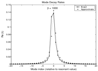
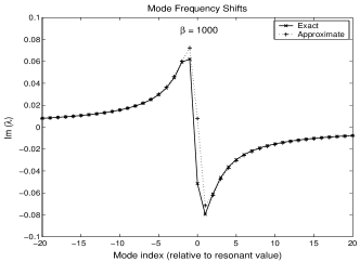
Figure 2: (a) Decay rates and (b) frequency detuning (from resonance) for the 40 fastest decaying modes, for $\beta=1000$, in units of $n_{0}\mu^{2}\beta/(3\hbar)$.

For further discussions of EM radiation from large spheres we undertake the development of the orthogonality properties of the EM eigenmodes. They are somewhat less self-evident than the analogous properties of the MM eigenmodes we considered in Sec. IV.

VI Orthogonality Properties of the Electric Multipole Modes

For the $n$th mode of the $(\ell m)$ order, which we shall call simply the $(\ell mn)$ mode, the magnetic field $\vec{B}^{(EM)}_{\ell mn}$ is given by Eq. (56), and the electric field $\vec{E}^{(EM)}_{\ell mn}$ essentially by its curl,

$$\vec{B}^{(EM)}_{\ell mn}={1\over ik_{0}\ell(\ell+1)}{\cal E}_{\ell mn}(r)\vec{L}Y_{\ell m}(\vec{\Omega}),$$ (79)

$$\vec{E}^{(EM)}_{\ell mn}={ik_{0}\over\gamma_{\ell n}^{2}}\vec{\nabla}\times\vec{B}^{(EM)}_{\ell mn}.$$ (80)

Let us first consider the orthogonality integral for the electric fields of two modes $p,p^{\prime}$ in two different multipole orders $(\ell,m)$ and $(\ell^{\prime},m^{\prime})$, with $\ell\neq\ell^{\prime}$:

$$\int_{r<R}\vec{E}^{(EM)}_{\ell mn}\cdot\vec{E}^{(EM)}_{\ell^{\prime}m^{\prime}n^{\prime}}d\vec{r}.$$

Use of Eq. (80) to replace the electric field $\vec{E}^{(EM)}_{\ell mn}$ in terms of the corresponding magnetic field $\vec{B}^{(EM)}_{\ell mn}$ and the identity

$$\vec{\nabla}\cdot(\vec{A}\times\vec{B})=\vec{B}\cdot\vec{\nabla}\times\vec{A}-\vec{A}\cdot\vec{\nabla}\times\vec{B},$$ (81)

followed by the use of Gauss’s theorem to reduce a total divergence term to a surface integral over the sphere, yields the result

$$\int_{r<R} \vec{E}^{(EM)}_{\ell mn}\cdot\vec{E}^{(EM)}_{\ell^{\prime}m^{\prime}n^{\prime}}d\vec{r}$$

$$={ik_{0}\over\gamma_{\ell n}^{2}}\int_{r=R}\vec{B}^{(EM)}_{\ell mn}\times\vec{E}^{(EM)}_{\ell^{\prime}m^{\prime}n^{\prime}}\cdot\hat{r}d^{2}S$$

$$-{k_{0}^{2}\over\gamma_{\ell n}^{2}}\int_{r<R}\vec{B}^{(EM)}_{\ell mn}\cdot\vec{B}^{(EM)}_{\ell^{\prime}m^{\prime}n^{\prime}}d\vec{r}.$$ (82)

Here Faraday’s law was employed in the last term to express the curl of $\vec{E}^{(EM)}_{\ell^{\prime}m^{\prime}n^{\prime}}$ in terms of the magnetic field $\vec{B}^{(EM)}_{\ell^{\prime}m^{\prime}n^{\prime}}$ of the $(\ell^{\prime}m^{\prime}n^{\prime})$ mode. That the last term in Eq. (VI) vanishes unless $\ell=\ell^{\prime}$ and $m=-m^{\prime}$ follows from the orthogonality of the different vector spherical harmonics $\vec{L}Y_{\ell m}$ in terms of which the magnetic fields of the two modes may be expressed by means of Eq. (79). By a similar but more detailed argument involving the identity Jackson1

$$i\vec{\nabla}\times\vec{L}=\vec{r}\nabla^{2}-\vec{\nabla}\left(1+r{\partial\over\partial r}\right),$$

we may reduce the surface integral in Eq. (VI) to a form involving $\int d^{2}\Omega\,\vec{L}Y_{\ell m}\cdot\vec{L}Y_{\ell^{\prime},m^{\prime}}$, which too vanishes unless $\ell=\ell^{\prime}$ and $m=-m^{\prime}$. This proves the orthogonality of the vector electric fields for modes with different $\ell$ and $m$ values.

A different approach is needed to establish orthogonality rules for modes with the same $\ell$ value. We begin with the field equations that $\vec{E}^{(EM)}_{\ell mn}$ and $\vec{E}^{(EM)}_{\ell m^{\prime}n^{\prime}}$ obey,

$$-ik_{0}\vec{\nabla}\times\vec{B}^{(EM)}_{\ell mn}+\gamma_{\ell n}^{2}\vec{E}^{(EM)}_{\ell mn}=0,$$ (83)

$$-ik_{0}\vec{\nabla}\times\vec{B}^{(EM)}_{\ell m^{\prime}n^{\prime}}+\gamma_{\ell n^{\prime}}^{2}\vec{E}^{(EM)}_{\ell m^{\prime}n^{\prime}}=0.$$ (84)

Taking the scalar product of Eq. (83) with $\vec{E}^{(EM)}_{\ell m^{\prime}n^{\prime}}$ and subtracting the result from that obtained on taking the scalar product of Eq. (84) with $\vec{E}^{(EM)}_{\ell mn}$, and integrating the difference over the spherical sample we secure the result

$$(\gamma_{\ell n}^{2}-\gamma_{\ell n^{\prime}}^{2})\int_{r<R}\vec{E}^{(EM)}_{\ell mn}\cdot\vec{E}^{(EM)}_{\ell m^{\prime}n^{\prime}}d\vec{r}$$

$$=ik_{0}\int_{r<R}\left[\vec{E}^{(EM)}_{\ell m^{\prime}n^{\prime}}\cdot\vec{\nabla}\times\vec{B}^{(EM)}_{\ell mn}\right.$$

$$\qquad\qquad-\left.\vec{E}^{(EM)}_{\ell mn}\cdot\vec{\nabla}\times\vec{B}^{(EM)}_{\ell m^{\prime}n^{\prime}}\right]d\vec{r}.$$ (85)

We now use the identity (81) to reexpress each term on the right hand side of Eq. (VI) in terms of a complete divergence, which reduces to a surface integral according to Gauss’s law, and a curl term, which from Faraday’s law can be written as a volume integral of $\vec{B}^{(EM)}_{\ell mn}\cdot\vec{B}^{(EM)}_{\ell m^{\prime}n^{\prime}}$. We see in this way that Eq. (VI) simplifies to a single surface integral, the two volume integrals canceling each other out,

$$(\gamma_{\ell n}^{2}-\gamma_{\ell n^{\prime}}^{2})\int_{r<R}\vec{E}^{(EM)}_{\ell mn}\cdot\vec{E}^{(EM)}_{\ell m^{\prime}n^{\prime}}d\vec{r}$$

$$=ik_{0}\int_{r=R}\left[(\hat{r}\times\vec{E}^{(EM)}_{\ell mn})\cdot\vec{B}^{(EM)}_{\ell m^{\prime}n^{\prime}}\right.$$

$$\qquad\qquad-\left.(\hat{r}\times\vec{E}^{(EM)}_{\ell m^{\prime}n^{\prime}})\cdot\vec{B}^{(EM)}_{\ell mn}\right]d^{2}S.$$ (86)

The surface integral involves only the tangential components of both the electric and magnetic fields, which are all continuous across the spherical boundary. The surface integral can, as such, be expressed equally well in terms of the same components of the free-space fields in the immediate exterior of the sphere. However, since in each multipole order $(\ell m)$ the exterior fields are all expressed in terms of the outgoing wave solutions $h_{\ell}^{(1)}(k_{0}r)Y_{\ell m}(\vec{\Omega})$ and their derivatives, independent of the mode indices $n,n^{\prime}$, the surface integral on the right hand side of Eq. (VI) vanishes identically. It follows then from Eq. (VI) that if $\gamma_{\ell n}\neq\gamma_{\ell n^{\prime}}$, then the orthogonality integral vanishes,

$$\int_{r<R}\vec{E}^{(EM)}_{\ell mn}\cdot\vec{E}^{(EM)}_{\ell m^{\prime}n^{\prime}}d\vec{r}\sim\delta_{nn^{\prime}}.$$ (87)

Combining all of the specific orthogonality relations we have discussed so far in this section, we may write down the overall orthogonality relation

$$\int_{r<R}\vec{E}^{(EM)}_{\ell mn}\cdot\vec{E}^{(EM)}_{\ell^{\prime}m^{\prime}n^{\prime}}d\vec{r}\sim\delta_{\ell\ell^{\prime}}\delta_{m,-m^{\prime}}\delta_{nn^{\prime}}.$$ (88)

This orthogonality relation (88) may also be directly established by using Eq. (79) and (80) to express its left hand side in terms of the mode functions ${\cal E}_{\ell mn}\sim j_{\ell}(\gamma_{\ell n}r)$, simplifying the resulting integral by means of angular momentum operator identities, and then exploiting the eigenvalue relation (64) that each mode must obey.

It is worth noting that the requirement $m=-m^{\prime}$, rather than $m=m^{\prime}$, for the nonvanishing of the expression (88) is a reminder of the symmetric but non-Hermitian character of the propagation kernel for the electromagnetic field. This nonhermiticity was already noted in II in the context of one-dimensional propagation when an incident wave with transverse magnetic polarization was obliquely incident on a slab.

VI.1 Expansion of an Arbitrary EM Field in the Corresponding Modes

The orthogonality integral (88) makes it possible to expand an arbitrary electromagnetic field in a particular EM order $(\ell,m)$ in terms of the EM modes, given by Eqs. (79) and (80), of the same order. Let $\vec{\nabla}\times[f(r)\vec{L}Y_{\ell m}]$ be an arbitrary field in this order expressed as the mode sum

$$\vec{\nabla}\times\left[f(r)\vec{L}Y_{\ell m}\right]=\sum_{n=1}^{\infty}f_{n}\vec{\nabla}\times\left[j_{\ell}(\gamma_{\ell n}r)\vec{L}Y_{\ell m}\right].$$ (89)

The coefficients $f_{n}$ are obtained by multiplying both sides of Eq. (89) by the mode function $\vec{\nabla}\times[j_{\ell}(\gamma_{\ell n^{\prime}}r)\vec{L}Y_{\ell,-m}]$, integrating over the spherical sample, and utilizing the orthogonality relation (88),

$$f_{n}={(j_{\ell}(\gamma_{\ell n}r),f(r))\over(j_{\ell}(\gamma_{\ell n}r),j_{\ell}(\gamma_{\ell n}r))},$$ (90)

where the symbol $(f,g)$ defines an inner product,

$$(f,g)\equiv\int_{r<R}d\vec{r}\left\{\vec{\nabla}\times[f(r)\vec{L}Y_{\ell,-m}]\right\}\cdot\left\{\vec{\nabla}\times[g(r)\vec{L}Y_{\ell m}]\right\}.$$ (91)

Whenever either $f$ or $g$ is a mode amplitude function $j_{\ell}(\gamma_{\ell n}r)$, the inner product (91) can be simplified greatly. To see this, we make use of formula (81) in Eq. (91) to transform its integrand to a term involving $\vec{\nabla}\times(\vec{\nabla}\times[g(r)\vec{L}Y_{\ell m}])$, which, when $g$ is a mode function, is simply $\gamma_{\ell n}^{2}g(r)\vec{L}\,Y_{\ell m}$, along with a pure divergence term, a term that from Gauss’s theorem is equal to a surface integral. Thus, when $g$ is a mode function, Eq. (91) takes a simpler form,

$$(f,g)=\gamma_{\ell n}^{2} \int_{r<R}f(r)g(r)\vec{L}Y_{\ell,-m}\cdot\vec{L}Y_{\ell m}d\vec{r}$$

$$+ \int f(r)\vec{L}Y_{\ell,-m}\times[\vec{\nabla}\times(g\vec{L}Y_{\ell m})]\cdot\hat{r}\,d^{2}S.$$

Use of the solid-angle integral identity

$$\int d^{2}\Omega\vec{L}Y_{\ell,-m}\cdot\vec{L}Y_{\ell m}=(-1)^{m+1}\ell(\ell+1)$$

and the fact Jackson1 that the surface integral in the preceding equation is simply $(-1)^{m+1}\ell(\ell+1)Rf(R)(d/dR)[Rg(R)]$ reduces the inner product (91) to the form

$$(f,g)=(-1)^{m+1} \ell(\ell+1)\left\{Rf(R){d\over dR}\left[Rg(R)\right]\right.$$

$$\left.+\gamma_{\ell n}^{2}\int_{0}^{R}f(r)g(r)r^{2}dr\right\}.$$ (92)

This form of the inner product can also be used as the starting point of a simple, direct proof of the orthogonality of different modes in a given multipole order.

VII Radiation from a Large Sphere with a Uniformly Excited Spherical Inner Core

Coherent radiation from a large resonant sphere will, in general, involve a large number of modes of both multipole types and their infinitely many orders. A particularly simple situation occurs, however, when an inner concentric spherical region of the sphere is uniformly excited initially, as shown in Fig. 3. This is a special case of a polarization with radially symmetric amplitude and uniform direction, which emits pure electric dipole radiation in the $(1,0)$ order.

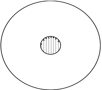
Figure 3: Spherical medium of radius $R$ with an excited concentric core of radius $r_{0}=fR$, $f\leq 1$.

Let us assume then an initial polarization of form

$$\vec{P}(\vec{r},0)=\begin{cases}\hat{z}P_{0}&{\rm for\ }r<r_{0}\\ 0&{\rm for\ }r_{0}<r<R.\end{cases}$$ (93)

The electric field that this polarization initially radiates has a simple expression in the rapid transit approximation PG00 in which retardation of slowly varying amplitudes is ignored and the second time derivatives in Eq. (16) are replaced by $-\omega^{2}$. In this approximation, the initial electric field $\vec{E}^{(+)}(\vec{r},0)$ may be expressed as an integral of the scalar product of the tensor propagator

$${\bf G}(\vec{r}-\vec{r}^{\,\prime})=\left({\bf 1}+{1\over k_{0}^{2}}\vec{\nabla}\vec{\nabla}\right){e^{ik_{0}|\vec{r}-\vec{r}^{\,\prime}|}\over 4\pi|\vec{r}-\vec{r}^{\,\prime}|}$$ (94)

and the initial polarization (93) over the spherical sample, which reduces to the form

$$\vec{E}(\vec{r},0)\approx P_{0}\left(k_{0}^{2}\hat{z}+{\partial\over\partial z}\vec{\nabla}\right)\int_{r^{\prime}<r_{0}}{e^{ik_{0}|\vec{r}-\vec{r}^{\,\prime}|}\over 4\pi|\vec{r}-\vec{r}^{\,\prime}|}d\vec{r}^{\,\prime}.$$ (95)

The initial field amplitude $d(r,0)$ is the radial function that multiplies the spherical harmonic $Y_{10}(\vec{\Omega})$ in the quantity $\vec{L}\cdot\vec{\nabla}\times\vec{E}(\vec{r},0)$. Taking the curl of the left hand side of Eq. (95) eliminates the pure gradient term,

$$\vec{\nabla}\times\vec{E}(\vec{r},0)=k_{0}^{2}P_{0}\vec{\nabla}\int_{r^{\prime}<r_{0}}{e^{ik_{0}|\vec{r}-\vec{r}^{\,\prime}|}\over 4\pi|\vec{r}-\vec{r}^{\,\prime}|}d\vec{r}^{\,\prime}\times\hat{z}.$$ (96)

By using the identity (27) to replace the integrand in Eq. (96) by a spherical harmonic sum and then integrating it over the angular coordinates, we see that the integral in Eq. (96) is a purely radial function,

$$f(r)=ik_{0}\int_{0}^{r_{0}}j_{0}(k_{0}r^{<})h_{0}^{(1)}(k_{0}r^{>})r^{\prime 2}dr^{\prime}.$$ (97)

We thus have the result

$$\vec{\nabla}\times\vec{E}(\vec{r},0)=k_{0}^{2}P_{0}\vec{\nabla}f(r)\times\hat{z}={df\over dr}{\vec{r}\over r}\times\hat{z}.$$

Operating on both sides of this equation by $\vec{L}\cdot$, noting that any function of $r$ commutes with $\vec{L}$, and using the result

$$\vec{L}\cdot(\vec{r}\times\hat{z}) ={1\over i}(\vec{r}\times\vec{\nabla})\cdot(\vec{r}\times\hat{z})$$

$$={1\over i}[\vec{r}\cdot(\hat{z}\cdot\vec{\nabla})\vec{r}-(\vec{r}\cdot\hat{z})(\vec{\nabla}\cdot\vec{r})]$$

$$=2i\vec{r}\cdot z=2ir\cos\theta=2i\sqrt{4\pi\over 3}rY_{10}(\vec{\Omega}),$$

we obtain

$$\vec{L}\cdot\vec{\nabla}\times\vec{E}(\vec{r},0)=d(r,0)Y_{10}(\vec{\Omega}),$$ (98)

where the initial field amplitude $d(r,0)$ takes the explicit form

$$d(r,0)=-2k_{0}^{3}\sqrt{4\pi\over 3}P_{0}{d\over dr}\int_{0}^{r_{0}}j_{0}(k_{0}r^{<})h_{0}^{(1)}(k_{0}r^{>})r^{\prime 2}dr^{\prime}.$$ (99)

The radial integral can also be performed in closed form by means of the indefinite-integral identities Schiff ,

$$\int j_{0}(x)x^{2}dx=x^{2}j_{1}(x),\ \ \ \int h_{0}^{(1)}(x)x^{2}dx=x^{2}h_{1}^{(1)}(x),$$ (100)

and its derivative taken by means of the identities

$${d\over dx}j_{0}(x)=-j_{1}(x),\ \ \ {d\over dx}h_{0}^{(1)}(x)=-h_{1}^{(1)}(x).$$ (101)

The following final form of the amplitude is obtained in this way:

$$d(r,0)=2k_{0}^{3}r_{0}^{2}\sqrt{4\pi\over 3}P_{0}j_{1}(k_{0}r_{0}^{<})h_{1}^{(1)}(k_{0}r_{0}^{>}),$$ (102)

where $r_{0}^{<}$ and $r_{0}^{>}$ are defined to be the smaller and the larger of the two radial distances $r$ and $r_{0}$, respectively.

The same steps that took us from Eq. (55) to Eq. (V.2) can be employed to write down the displacement field envelope $\vec{D}(\vec{r},t)$ in terms of the amplitude $d(r,t)$ of electric dipole radiation $(\ell=1)$,

$$\vec{D}(\vec{r},t)\approx{1\over 2k_{0}^{2}}\vec{\nabla}\times[d(r,t)\vec{L}Y_{10}(\vec{\Omega})].$$ (103)

Inside the medium, the amplitude $d(r,t)$ may be expanded in terms of the mode functions $j_{1}(\gamma_{n}r)\exp(-\lambda_{n}t)$,

$$d(r,t)=\sum_{n=1}^{\infty}d_{n}j_{1}(\gamma_{n}r)\exp(-\lambda_{n}t).$$ (104)

Orthogonality of the mode functions under the inner product (VI.1) enables us to solve for the coefficients,

$$d_{p}={(d(r,0),j_{1}(\gamma_{n}r))\over(j_{1}(\gamma_{n}r),j_{1}(\gamma_{n}r))}.$$ (105)

The inner products in Eq. (105) contain integrals involving bilinear expressions of spherical Bessel and Hankel functions of the same order 1, which, as we show in Appendix A, can be evaluated in terms of simple trigonometric functions. The inner product in the numerator assumes the form,

$$(d(r,0),j_{1}(\gamma_{n}r))=-4ik_{0}^{2}r_{0}^{2}\sqrt{4\pi\over 3}P_{0}{\gamma_{n}^{2}\over k_{0}^{2}-\gamma_{n}^{2}}j_{1}(\gamma_{n}r_{0}),$$

while that in the denominator greatly simplifies in the limit of large $|\gamma_{n}|R$,

$$(j_{1}(\gamma_{n}r),j_{1}(\gamma_{n}r))\approx-R,$$

so the amplitude $d_{n}$ may be expressed as

$$d_{n}\approx 4i{k_{0}^{2}r_{0}^{2}\over R}\sqrt{4\pi\over 3}P_{0}{\gamma_{n}^{2}\over k_{0}^{2}-\gamma_{n}^{2}}j_{1}(\gamma_{n}r_{0}).$$ (106)

The electric field envelope $\vec{E}(\vec{r},t)$ has a similar form as the electric displacement field $\vec{D}(\vec{r},t)$,

$$\vec{E}(\vec{r},t)\approx{1\over 2k_{0}^{2}}\vec{\nabla}\times[e(r,t)\vec{L}Y_{10}(\vec{\Omega})],$$ (107)

with the amplitude $e(r,t)$ having a similar mode decomposition as $d(r,t)$,

$$e(r,t)=\sum_{n=1}^{\infty}n_{p}j_{1}(\gamma_{n}r)\exp(-\lambda_{n}t).$$ (108)

The mode coefficient $e_{n}$ for the electric field is obtained from $d_{n}$, the analogous coefficient for the displacement field, by dividing the latter by the dielectric constant $\gamma_{n}^{2}/k_{0}^{2}$ for the $n$th mode,

$$e_{n}={d_{n}\over(\gamma_{n}/k_{0})^{2}}\approx 4i{k_{0}^{2}r_{0}^{2}\over R}\sqrt{4\pi\over 3}P_{0}{k_{0}^{2}\over k_{0}^{2}-\gamma_{n}^{2}}j_{1}(\gamma_{n}r_{0}).$$ (109)

The resonant character of the excitation of the modes is unmistakable in the denominator of the right hand side of Eq. (109) – only modes with propagation constants $\gamma_{n}$ that are closely matched to the free space wave vector $k_{0}$ are preferentially excited. Also, because $j_{1}(\gamma_{n}r_{0})$ falls off rapidly with $\gamma_{n}$ for $|\gamma_{n}|r_{0}>>1$, only modes with propagation constants of order $1/r_{0}$ or smaller in magnitude are significantly excited in the preparation of the initial core excitation.

VII.1 Frequency Spectrum of Radiation

The initial polarization (93) radiates light into the various electric-field eigenmodes with amplitudes $e_{n}$. Apart from overall angular and distance dependences, the spectral amplitude of radiation, $a(R,{\delta\omega})$, at detuning ${\delta\omega}$ is given by the Fourier transform of the electric field amplitude $e(R,t)$ at the surface of the sphere,

$$a({\delta\omega})=\int_{0}^{\infty}e(R,t)e^{i{\delta\omega}t}dt=\sum_{n=1}^{\infty}{e_{n}j_{1}(\gamma_{n}R)\over\lambda_{n}-i{\delta\omega}}.$$ (110)

By substituting for $e_{n}$ from Eq. (109) and using the relation (35) between $\gamma_{\lambda}$ and $\lambda$ in Eq. (109), we may express the spectral amplitude as

$$a({\delta\omega})=4{k_{0}^{2}r_{0}^{2}\over R}\sqrt{4\pi\over 3}P_{0}{\beta^{2}\over{\delta\omega}}\sum_{n}{j_{1}(\gamma_{n}r_{0})j_{1}(\gamma_{n}R)\over\gamma_{n}^{2}R^{2}-\beta^{2}_{\delta\omega}},$$ (111)

where $\beta_{\delta\omega}$ is $R$ times the propagation constant for a plane wave of frequency $(\omega_{0}+{\delta\omega})$ traversing the medium,

$$\beta_{\delta\omega}=\beta\sqrt{1-{n_{0}|\vec{\mu}|^{2}/(3\hbar)\over{\delta\omega}}}.$$ (112)

The power spectrum of radiation is obtained from $a({\delta\omega})$ by taking its squared modulus.

The mode sum of Eq. (111) may be evaluated numerically. However, because of its resonant character which implies significant contribution from only those modes that have propagation constant close to the plane-wave propagation constant $\beta_{\delta\omega}$, accurate analytical approximations are also possible. First of all, for large spheres, $\beta>>1$, since all of the mode propagation constants $\gamma_{n}$ are largely real with relatively small imaginary parts, there is little radiation at frequency detunings that lie in the range $(0,n_{0}|\vec{\mu}|^{2}/(3\hbar))$ for which $\beta_{\delta\omega}$ is purely imaginary. Due to a strong resonant interaction of light with matter, radiation simply cannot propagate far in this frequency range. There is thus a gap in the spectrum in this range, a feature of resonant radiation that was already noted in the one-dimensional problem PG00 .

Outside this gap, the propagation constant $\beta_{\delta\omega}$ is either large or small compared to the radius parameter $\beta$, and the following excellent analytical approximations can be verified for the propagation constants $\gamma_{n}$ of the significantly contributing modes, those for which $|\gamma_{n}|R\approx\beta_{\delta\omega}$:

$$x_{n}= \gamma_{n}R$$

$$\approx \begin{cases}\left(n-{1\over 2}\right)\pi-i{\displaystyle{\beta\over\left(n-{1\over 2}\right)\pi}}&{\rm for\ }{\delta\omega}<0\\ n\pi-i{\displaystyle{n\pi\over\beta}}&{\rm for\ }{\delta\omega}>n_{0}|\vec{\mu}|^{2}/(3\hbar).\end{cases}$$ (113)

When these expressions are substituted in the resonant denominators of the terms in the mode sum (111) and in the large-argument approximation for $j_{1}(\gamma_{n}R)$, namely $-\cos(\gamma_{n}R)/(\gamma_{n}R)$, and $\gamma_{n}R$ is replaced by $\beta_{\delta\omega}$ in terms that vary slowly from one mode to the next, the following analytical forms result for the spectral amplitude:

$$a({\delta\omega})\approx -4{k_{0}^{2}r_{0}^{2}\over R}\sqrt{4\pi\over 3}P_{0}{\beta^{2}j_{1}(\beta_{\delta\omega}f)\over{\delta\omega}\beta_{\delta\omega}}$$

$$\times\begin{cases}-i\beta{\displaystyle\sum_{n=1}^{\infty}{(-1)^{n}\over(n-1/2)\pi\,[(n-1/2)^{2}\pi^{2}-\gamma_{\delta\omega}^{2}]}}&{\rm for\ }{\delta\omega}<0\\ {\displaystyle\sum_{n=1}^{\infty}{(-1)^{n}\over n^{2}\pi^{2}-\gamma_{\delta\omega}^{2}}}&{\rm for\ }{\delta\omega}>n_{0}|\vec{\mu}|^{2}/(3\hbar),\end{cases}$$ (114)

where $f=r_{0}/R$ denotes the fraction of the spherical radius initially excited and $\gamma_{\delta\omega}$ an effective propagation constant that takes slightly different forms below and above the gap,

$$\gamma_{\delta\omega}=\begin{cases}\sqrt{\beta_{\delta\omega}^{2}+2i\beta}&{\rm for\ }{\delta\omega}<0\\ \beta_{\delta\omega}(1+i/\beta)&{\rm for\ }{\delta\omega}>n_{0}|\vec{\mu}|^{2}/(3\hbar).\end{cases}$$ (115)

An overall factor that differs from 1 by terms of order $1/\beta$ has been dropped from Eq. (VII.1) which is bound to be accurate for large values of $\beta$ only. Both sums in Eq. (VII.1) may be evaluated in closed form. The second sum is well known GR65 . The evaluation of the first sum by means of contour integration is presented in Appendix B. The following closed-form expressions are then obtained for the spectral amplitude below and above the frequency gap:

$$a({\delta\omega}) \approx 4{k_{0}^{2}r_{0}^{2}\over R}\sqrt{4\pi\over 3}P_{0}{\beta^{2}j_{1}(\beta_{\delta\omega}f)\over{\delta\omega}\beta_{\delta\omega}}$$

$$\times\begin{cases}-{\displaystyle{i\beta\over 2\gamma_{\delta\omega}^{2}}\left(1-{1\over\cos\gamma_{\delta\omega}}\right)}&{\rm for\ }{\delta\omega}<0\\ {\displaystyle{1\over 2\gamma_{\delta\omega}}\left({1\over\sin\gamma_{\delta\omega}}-{1\over\gamma_{\delta\omega}}\right)}&{\rm for\ }{\delta\omega}>{n_{0}|\vec{\mu}|^{2}\over 3\hbar}.\end{cases}$$ (116)

The squared modulus $S({\delta\omega})=|a({\delta\omega})|^{2}$ represents the power spectral density of radiation.

We plot in Figs. 4 the power spectrum $S({\delta\omega})$ for a variety of values of $\beta$ and the fractional excited radius $f\equiv r_{0}/R$. For small spherical samples with linear dimensions comparable to the wavelength of light, as for $\beta=1$, coherent radiation initially proceeds by the fast decaying superradiant mode we discussed in Sec. II, but the relatively slowly decaying modes that we discussed in Sec. V.B.1 continue to radiate for long periods of time. Because of the simple proportionality of the decay rate to the width of the spectrum radiated by a mode, the superradiant mode furnishes a broad spectral background on which are coherently superposed sharper line spectra corresponding to the slowly decaying modes. Each spectral peak corresponding to a mode is centered at a frequency detuning equal to the imaginary part of the decay constant of that mode. We display the power spectrum of emitted radiation for four different values of the fractional excited core radius, $f$, namely 0.1, 0.5, 0.75, and 1, in Figs. 4(a)-(d). Since the more localized initial excitations are made up of a larger number of weakly decaying modes, all superposed coherently with the fundamental supperradiant mode, the overall power spectrum consists of a broad peak and a fine structure of ever narrower peaks that accumulate below zero detuning, as seen most dramatically in Fig. 4(d). An initial excitation of the full sphere corresponds, by contrast, to only a small admixture of the weakly decaying modes, that are visible in Fig. 4(a) as small peaks on the broad background provided by the superradiant mode. When considered in sequence, these four subplots also illustrate how even for small values of $\beta$ a frequency gap develops over the interval $[0,n_{0}\mu^{2}/(3\hbar)]$ as the initial excitation of the sphere is more and more tightly confined close to its center. The broad background contribution of the superradiant mode gets progressively smaller, yielding little power at any positive frequency detuning including this gap.

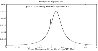
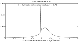
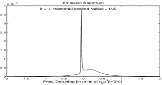
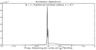
Figure 4: The frequency spectrum of the power radiated by the medium, in arbitrary units, as a function of the frequency detuning, in units of $n_{0}|\vec{\mu}|^{2}\beta/(3\hbar)$, for $\beta=1$, with (a) $f=1$ (uniform initial excitation); (b) $f=0.75$; (c) $f=0.5$; and (d) $f=0.1$

For larger spheres too, a similar fine structure is obtained in the spectrum, but the emergence of a well defined frequency gap we discussed earlier is unmistakable with $\beta$ increasing in value from 10 to 100, as we see in Figs. 5 and 6. The more localized the initial excitation the more prominent the peaks to the left of the gap. This is a result of the fact that the peaks with negative detuning correspond to modes that have propagation constants that are large compared to $k_{0}$ and which are therefore needed to make up an excitation that is localized on the sub-wavelength scale corresponding to $\beta f<<1$. The analytical approximation (VII.1), shown by a dashed curve on each plot, is already accurate for $\beta=10$, and is nearly indistinguishable from the numerically exact results for $\beta=100$. For $\beta=10$ the most superradiant mode has a decay rate that, according to expression (78), is a factor $\ln\beta=2.3$ times smaller than $n_{0}\mu^{2}\beta/(3\hbar)$. This accounts for the considerably narrower background provided by this mode to the emission spectrum in Fig. 5(a) than that present in Fig. 4(a) for $\beta=1$, even though that mode dominates the other modes when the sphere is uniformly excited. For much larger values of $\beta$, as in Figs. 6, the superradiant modes, which are of order $(\ln\beta)/\pi$ in number, each correspond to a spatially nonuniform excitation given by Eq. (53) with $\gamma_{\lambda}R\sim\beta$. A uniformly excited core, regardless of its fractional radius, $f$, is thus comprised of large numbers of superradiant and weakly decaying modes, which always yield a rich spectrum of narrow peaks that accumulate on either side of the frequency gap.

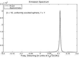
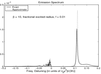
Figure 5: Same as Fig. 4(a), except (a) $\beta=10$, $f=1$ and (b) $\beta=10$, $f=0.01$.

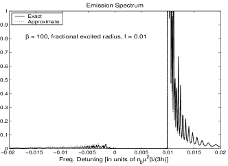
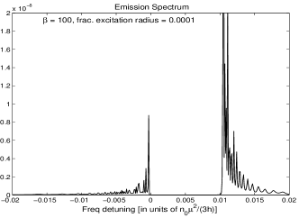
Figure 6: Same as Figs. 5(a), except (a) $\beta=100$, $f=0.01$ and (b) $\beta=100$, $f=0.0001$.

VII.2 Time Dependence of the Radiated Power

The power $dW/dt$ radiated by the resonantly excited sphere is given by integrating the normal component of the Poynting vector over the surface of the sphere. For $\beta>>1$, this integral may be reduced to a rather simple final form, as we show in Appendix C,

$${dW\over dt}=-{c\beta^{4}\over k_{0}^{4}(1+\beta^{2})}|d(R,t)|^{2},$$ (117)

where $d(R,t)$ is the amplitude function that determines the electric displacement field at the spherical surface, $r=R$, via relation (104).

VII.2.1 Radiation from a Large Sphere, $\beta>>1$, with a Small Excited Core, $f<<1$

The early stages of radiation are dominated by the fast-decaying, superradiant modes, while the excitation residing in the more weakly radiating modes is slow to escape the medium. The latter are accompanied by an oscillatory exchange of energy between the atoms and the radiation field, as we shall see presently. Similar attributes of cooperative emission from extended media have also been seen for a symmetric Dicke one-photon excitation SS091 ; M09 .

If we use in expression (106) the approximate eigenvalue formulas (77) and (78), valid for the superradiant modes of a large sphere, and then evaluate the sum (104), we are assured of good accuracy for the times when those modes are the ones actively radiating. Since the superradiant modes have propagation constants that do not differ much from the free-space one, $k_{0}$, we first approximate $(k_{0}^{2}-\gamma_{n}^{2})$ by 2$k_{0}(k_{0}-\gamma_{n})$, $\gamma_{n}^{2}$ by $k_{0}^{2}$, and then substitute formulas (77) and (78) in the expression (106). We assume here a small initially excited core, $r_{0}<<R$, so we may replace $j_{1}(\gamma_{n}r_{0})$ by $j_{1}(\beta f)$, while the large-argument approximation for $j_{1}(\gamma_{n}R)$ coupled with expression (77) reduces it to the form

$$j_{1}(\gamma_{n}R)\approx-{\cos\gamma_{n}R\over\gamma_{n}R}\approx(-1)^{n+1}{e^{i\pi/4}\over\sqrt{\beta}},$$ (118)

where we used $\beta>>1$ to ignore a term of relative order $1/\beta$ and replaced $\gamma_{n}R$ in the denominator simply by $\beta$. With these approximations and upon extending the sum (104) to also include all negative integral values of the index $n$, which adds spurious terms to the sum that we later subtract out approximately, we may express the field amplitude $d(R,t)$ at the surface of the sphere as

$$d(R,t)= -ie^{i\pi/4}\sqrt{4\pi\over 3}{f^{2}\beta^{2}}j_{1}(\beta f)P_{0}$$

$$\times\sum_{n=-\infty}^{\infty}{(-1)^{n}e^{\displaystyle{i\alpha t/[n\pi-\beta-(i/2)\ln\beta]}}\over[n\pi-\beta-(i/2)\ln\beta]},$$ (119)

This sum may be evaluated exactly by the method of contour integrals in the complex plane, as shown in Appendix D, and the following asymptotic expansion in powers of $1/\beta$ is obtained:

$$d(R,t)= 2e^{i\pi/4}\sqrt{4\pi\over 3}{f^{2}\beta^{2}}j_{1}(\beta f)P_{0}{e^{i\beta}\over\sqrt{\beta}}$$

$$\times\sum_{n=0}^{\infty}\left({e^{2i\beta}\over\beta}\right)^{n}J_{0}(2\sqrt{(2n+1)\alpha t}),$$ (120)

where $J_{0}$ denotes Bessel function of the first kind of order 0. For large values of $\beta$, the first term alone suffices to furnish an accurate result for $d(R,t)$ and thus for the radiated power (111),

$${dW\over dt}\approx-{16\pi\over 3}\omega_{0}k_{0}r_{0}^{4}[j_{1}(\beta f)]^{2}|P_{0}|^{2}J_{0}^{2}(2\sqrt{\alpha t}).$$ (121)

The oscillatory time dependence (121) of the radiated power represents an exchange of energy between the field and the polarization of the radiating medium. Such oscillatory energy exchange is characteristic of any radiation problem in which many modes of comparable decay rates that are detuned by different amounts from the resonance frequency participate coherently. A squared Bessel function time dependence related to Eq. (121) was first derived by Burnham and Chiao BC69 in the one-dimensional context of radiation from a semi-infinite medium that is coherently generated in the wake of a sweeping $\delta-$function excitation pulse.

An expression for the radiated power that is somewhat more accurate than Eq. (121) is given by subtracting out the spurious terms, those with $n$ running from 0 to $-\infty$, that we included in the sum (VII.2.1) in order to derive the Bessel-function result (VII.2.1). Because of their non-resonant character, the sum of these spurious terms can be evaluated approximately, as we show in Appendix E, and subtracted from Eq. (VII.2.1). This procedure yields the following two-term result for the radiated power:

$${dW\over dt}\approx -{16\pi\over 3}\omega_{0}k_{0}r_{0}^{4}[j_{1}(\beta f)]^{2}|P_{0}|^{2}\Bigg{[}J_{0}^{2}(2\sqrt{\alpha t})$$

$$-{1\over 2\sqrt{\beta}}J_{0}(2\sqrt{\alpha t})\sin(\beta+\alpha t/\beta)e^{-\displaystyle{{\alpha t\over 2\beta^{2}}\ln\beta}}\Bigg{]}.$$ (122)

In Figs. 7-9, we plot the power radiated by a spherical medium for the same values of the radius parameter $\beta$ for which the radiated spectrum was considered in Figs. 4-6. For a uniformly excited sphere ($f=1$) with $\beta=1$, the fundamental superradiant mode is nearly the only one excited, which implies a purely exponential decay of the radiated power, as seen in Fig. 7(a). When the medium is initially excited from the center out to only a tenth of the radius, as in Fig. 7(b), a significant number of weakly decaying modes of comparable magnitude are present as well. The initial precipitous drop in power results from the decay of the superradiant mode, but the subsequent emission has an oscillatory time dependence due to radiation emitted coherently by the weakly decaying modes. The oscillations are slow with a long quasi-period, due to rather small differences in the frequency detunings of these modes, as we noted earlier.

Figure 7: The power radiated by the medium, in arbitrary units, as a function of time, in units of $[n_{0}|\vec{\mu}|^{2}\beta/(3\hbar)]^{-1}$, for $\beta=1$ with (a) $f=1.0$ and (b) $f=0.1$.

As we increase the value of $\beta$, we find inevitably the emergence of an oscillatory time dependence for power that for early times is described approximately by the Bessel function result (VII.2.1). This is particularly accurate for the larger value, 100, of $\beta$ when the fractional excited core radius, $f$, is small, as seen in Figs. 9(b). The approximate result (VII.2.1) ceases, however, to agree with the numerically exact behavior at long times due to the fact that the former wrongly presupposes that the superradiant modes continue to dominate the radiation for all times. In reality, the weakly decaying modes continue to radiate for long times, well after the superradiant modes have radiated away nearly all of their excitation. The differences between the frequencies of neighboring modes, that determine the detailed character of the temporal oscillations, are dissimilar for the two varieties of modes, accounting for the failure of the approximate result (VII.2.1) to describe the long-time behavior of the radiated power. It is worth noting that times greatly exceeding those plotted would be necessary to see the stretched exponential decay of polarization energy predicted in the one-dimensional problem of localized excitation PG00 .

Figure 8: Same as Figs. 7(a) and (b), except (a) $\beta=10$, $f=1.0$ and (b) $\beta=10$, $f=0.01$.

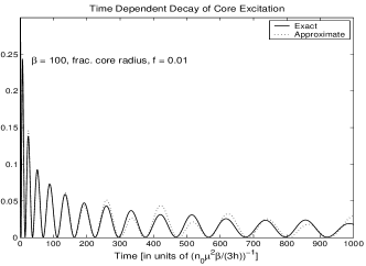
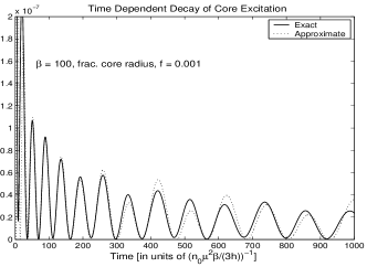
Figure 9: Same as Figs. 7(a) and (b), except (a) $\beta=100$, $f=0.01$ and (b) $\beta=100$, $f=0.001$.

VIII Concluding Remarks

Coherent radiation from a sphere of polarizable atoms with a single resonant excitation energy level can exhibit a rich variety of spectral and temporal characteristics. A fully excited sphere with uniform polarization radiates much like a single atom, when its radius is small compared to the wavelength of emission. When coherently excited, a large sphere, by contrast, almost always radiates a superposition of strongly decaying, or superradiant, and weakly decaying, or subradiant, modes. These exponentially decaying modes may be classified as magnetic and electric multipole modes of various angular momentum orders. A particularly simple, yet sufficiently general, case of our problem is that of radiation from a uniformly excited concentric spherical core within an otherwise unexcited spherical medium. We have demonstrated that such an excitation radiates as a pure electric dipole, regardless of the size of the medium or its excited core. This specific case has been studied in detail in the present paper.

The characteristic differences between the frequency detunings and decay rates of the modes give rise to radiation that has a wealth of sharp peaks and valleys in its spectrum. It also has a frequency range in which radiation cannot propagate far because of its strong resonant interaction within the medium, and is thus unable to escape it. We derived an analytical approximation of this spectrum that involves simple trigonometric functions and is highly accurate for large values of $\beta$. The time dependence is correspondingly quite involved, with a complicated oscillatory behavior that persists for long times. For times that are not too long, a simple analytical result based on the inclusion of superradiant modes alone furnishes a good approximation to the exact time dependence. Many of these characteristics of emission, previously noted in our treatment of the one-dimensional coherent radiation problem as well, are likely to survive the change of geometry, provided geometrical length scales remain large compared to the characteristic wavelengths of emission. A well localized excitation deep in the interior of an extended medium of arbitrary geometry will, for example, remain trapped for long periods of time, releasing energy only slowly, unless incoherent processes intervene.

Appendix A Evaluation of the Inner Products in Eq. (99)

When expression (102) for $d(r,0)$ is substituted into the inner product formula (86), we obtain

$$(d(r,0), j_{1}(\gamma_{n}r))=-4k_{0}^{3}r_{0}^{2}\sqrt{4\pi\over 3}P_{0}$$

$$\times\Big{\{}Rj_{1}(k_{0}r_{0})h^{(1)}_{1}(k_{0}R)[Rj_{1}(\gamma_{n}R)]^{\prime}$$

$$\qquad+\gamma_{n}^{2}\int_{0}^{R}r^{2}h^{(1)}_{1}(k_{0}r^{>})j_{1}(k_{0}r^{<})j_{1}(\gamma_{n}r)dr\Big{\}},$$ (123)

where a prime superscript denotes a derivative with respect to the radial coordinate, here $R$. Since $r^{>}$ is the larger of $r,r_{0}$ and $r^{<}$ the smaller, to evaluate the integral in Eq. (A1), we write it as a sum of two integrals

$$h_{1}^{(1)}(k_{0}r_{0}) \int_{0}^{r_{0}}r^{2}j_{1}(k_{0}r)j_{1}(\gamma_{n}r)dr$$

$$+j_{1}(k_{0}r_{0})\int_{r_{0}}^{R}r^{2}h^{(1)}_{1}(k_{0}r^{)}j_{1}(\gamma_{n}r)dr.$$ (124)

Indefinite integrals of the form $\int z_{\ell}(\alpha r)w_{\ell}(\beta r)r^{2}dr$, where $z_{\ell}$ and $w_{\ell}$ are any two spherical Bessel functions of order $\ell$, can be computed analytically. To see how, we first recognize that Bessel functions obey appropriate Bessel differential equations,

$$[rz_{\ell}(\alpha r)]^{\prime\prime}+[\alpha^{2}-\ell(\ell+1)/r^{2}][rz_{\ell}(\alpha r)]=0,$$ (125)

$$[rw_{\ell}(\beta r)]^{\prime\prime}+[\beta^{2}-\ell(\ell+1)/r^{2}][rw_{\ell}(\beta r)]=0.$$ (126)

By multiplying Eq. (125) by $rw_{\ell}(\beta r)$ and Eq. (126) by $rz_{\ell}(\alpha r)$, then subtracting one resulting equation from the other, and finally integrating both sides over $r$ followed by a simple rearrangement of terms, we obtain

$$\int r^{2}z_{\ell}(\alpha r)w_{\ell}(\beta r)r^{2}dr= {1\over(\alpha^{2}-\beta^{2})}$$

$$\times\int dr[rz_{\ell}(rw_{\ell})^{\prime\prime}-rw_{\ell}(rz_{\ell})^{\prime\prime}].$$ (127)

Since the integrand of the right hand side of Eq. (A) is the derivative of $[rz_{\ell}(rw_{\ell})^{\prime}-rw_{\ell}(rz_{\ell})^{\prime}]$, its integral is trivially evaluated, and Eq. (A) reduces to the form

$$\int r^{2}z_{\ell}(\alpha r)w_{\ell}(\beta r)r^{2}dr={1\over(\alpha^{2}-\beta^{2})}[rz_{\ell}(rw_{\ell})^{\prime}-rw_{\ell}(rz_{\ell})^{\prime}].$$ (128)

The indefinite-integral formula (128) may now be used to compute the two definite integrals in expression (A), and thus the integral in Eq. (A) for which the following expression results:

$$\int_{0}^{R} r^{2}h^{(1)}_{1}(k_{0}r^{>})j_{1}(k_{0}r^{<})j_{1}(\gamma_{n}r)dr$$ (129)

$$= {1\over(k_{0}^{2}-\gamma_{n}^{2})}\Big{\{}j_{1}(k_{0}r_{0})\left[Rh_{1}^{(1)}(k_{0}R)(Rj_{1}(\gamma_{n}R))^{\prime}-Rj_{1}(\gamma_{n}R)(Rh_{1}^{(1)}(k_{0}R))^{\prime}\right]$$

$$+ j_{1}(\gamma_{n}r_{0})\left[r_{0}j_{1}(k_{0}r_{0})(r_{0}h^{(1)}_{1}(k_{0}r_{0}))^{\prime}-r_{0}h^{(1)}_{1}(k_{0}r_{0})(r_{0}j_{1}(k_{0}r_{0}))^{\prime}\right]\Big{\}}.$$

Use of a Wronskian identity turns the terms within the second pair of brackets in Eq. (129) into $i/k_{0}$, while the terms within the first pair of brackets can be combined in view of the eigenvalue relation (64). These simplifications reduce Eq. (129) to the form

$$\int_{0}^{R} r^{2}h^{(1)}_{1}(k_{0}r^{>})j_{1}(k_{0}r^{<})j_{1}(\gamma_{n}r)dr={1\over(k_{0}^{2}-\gamma_{n}^{2})}$$ (130)

$$\times\Big{\{} j_{1}(k_{0}r_{0})Rh_{1}^{(1)}(k_{0}R)[Rj_{1}(\gamma_{n}R)]^{\prime}(1-k_{0}^{2}/\gamma_{n}^{2})$$

$$+ (i/k_{0})j_{1}(\gamma_{n}r_{0})\Big{\}}.$$

When the integral (130) is substituted into the right hand side of Eq. (A), the inner product attains its final form

$$(d(r,0),j_{1}(\gamma_{n}r))=-4ik_{0}^{2}r_{0}^{2}\sqrt{4\pi\over 3}P_{0}{\gamma_{n}^{2}\over(k_{0}^{2}-\gamma_{n}^{2})}j_{1}(k_{0}r_{0}).$$ (131)

The inner product $(j_{1}(\gamma_{n}r),j_{1}(\gamma_{n}r))$ involves, as definition (86) indicates, the integral

$$\int_{0}^{R}drj_{1}^{2}(\gamma_{n}r)dr,$$

which can be evaluated exactly in closed form by means of the indefinite-integral identity Schiff

$$\int x^{2}j_{1}^{2}(x)dx={x^{3}\over 2}[j_{1}^{2}(x)-j_{0}^{2}(x)j_{2}^{2}(x)].$$

This yields the following exact result for the inner product:

$$(j_{1}(\gamma_{n}r),j_{1}(\gamma_{n}r))={-2\over\gamma_{n}} \Big{\{}xj_{1}(x)[xj_{1}(x)]^{\prime}$$

$$+{x^{3}\over 2}[j_{1}^{2}(x)-j_{0}^{2}(x)j_{2}^{2}(x)]\Big{\}},$$ (132)

where $x=\gamma_{n}R$. By substituting the explicit trigonometric forms for the spherical Bessel functions of orders 0,1,2,

$$j_{0}(x) ={\sin x\over x},\ \ j_{1}(x)={\sin x\over x^{2}}-{\cos x\over x},$$

$$j_{2}(x) =\left({3\over x^{3}}-{1\over x}\right)\sin x-{3\over x^{2}}\cos x,$$

and performing simple algebraic manipulations, we may reduce Eq. (A) to the form

$$(j_{1}(\gamma_{n}r),j_{1}(\gamma_{n}r))={-1\over\gamma_{n}} \left[x-\left(1-{4\over x^{2}}\right)\sin x\,\cos x\right.$$

$$-\left.{2\over x}\cos x-{2\over x^{3}}\sin x\right].$$ (133)

For large $|x|=|\gamma_{n}|R$, only the first term in the square brackets in Eq. (A) is important,

$$(j_{1}(\gamma_{n}r),j_{1}(\gamma_{n}r))\approx-R,\ \ \ \ |\gamma_{n}|R>>1,$$ (134)

which is the expression used in arriving at Eq. (106).

Appendix B Evaluation of the First Sum in Eq. (VII.1)

Consider the contour integral

$$I(\alpha)\equiv\oint_{C}{dz\over z(z-\alpha)\cos z},$$ (135)

where the contour $C$ may be taken to be a circle of radius $N\pi$ in the complex-$z$ plane. Take $N$ to be a positive integer and $\alpha$ to be a finite complex number. In the limit $N\to\infty$, the integral (135) must vanish, since the integrand goes to zero faster than $1/N^{2}$ while $dz$ grows only linearly with $N$. But, by the residue theorem, the integral on the RHS is simply $2\pi i$ times the sum of residues of the integrand at all of its poles in the finite complex plane. In the limit $N\to\infty$, the integrand has only simple poles at 0, $\alpha$, and $(n-1/2)\pi$, $n=0,\pm 1,\pm 2,\ldots$, where the residues are easily evaluated, and the following sum formula results:

$$0=2\pi i\left\{{-1\over\alpha}+{1\over\alpha\,\cos\alpha}-\sum_{n=-\infty}^{\infty}{1\over(n-1/2)\pi[(n-1/2)\pi-\alpha]\sin(n-1/2)\pi}\right\}.$$ (136)

Note that $\sin(n-1/2)\pi=(-1)^{n-1}$. The infinite sum may be re-expressed as a one-sided sum by relabeling $n$ by $(1-n^{\prime})$ in the part of the sum that is over $n=-\infty$ to 0 and then dropping the prime from $n^{\prime}$, as shown below:

$$\sum_{n=-\infty}^{\infty}{(-1)^{n}\over(n-1/2)[(n-1/2)\pi-\alpha]} = \sum_{n=1}^{\infty}{(-1)^{n}\over(n-1/2)[(n-1/2)\pi-\alpha]}+\sum_{n^{\prime}=1}^{\infty}{(-1)^{1-n^{\prime}}\over(1/2-n^{\prime})[(1/2-n^{\prime})\pi-\alpha]}$$

$$= \sum_{n=1}^{\infty}{(-1)^{n}\over(n-1/2)}\left[{1\over(n-1/2)\pi-\alpha}-{1\over(n-1/2)\pi+\alpha}\right]$$

$$= 2\alpha\sum_{n=1}^{\infty}{(-1)^{n}\over(n-1/2)[(n-1/2)^{2}\pi^{2}-\alpha^{2}]}.$$

When this result is substituted into Eq. (136), we obtain a closed-form expression for the sum needed in Eq. (VII.1), namely

$$\sum_{n=1}^{\infty}{(-1)^{n}\over(n-1/2)\pi[(n-1/2)^{2}\pi^{2}-\alpha^{2}]}={1\over 2\alpha^{2}}\left(1-{1\over\cos\alpha}\right).$$ (137)

Appendix C Cycle-Averaged Radiated Power

When averaged over the fundamental oscillation period, $2\pi/\omega_{0}$, the Poynting vector takes the form

$$\vec{S}(\vec{r},t)=2c\ {\rm Re}\left[\vec{E}(\vec{r},t)\times\vec{B}^{*}(\vec{r},t)\right].$$ (138)

The integral of the normal component of $\vec{S}$ over the surface of the sphere, $r=R$, gives the total cycle-averaged power, $-dW/dt$, radiated by the sphere at time t,

$$-{dW\over dt}=R\int d^{2}\Omega\,\vec{r}\cdot\vec{S}|_{r=R}.$$ (139)

The electric field $\vec{E}$ is given by the expression (107)), while the magnetic field $\vec{B}$, which obeys the Maxwell equation

$$\vec{D}={i\over k_{0}}\vec{\nabla}\times\vec{B},$$

may be read off from Eq. (103) for $\vec{D}$,

$$\vec{B}(\vec{r},t)={1\over 2ik_{0}}d(r,t)\vec{L}Y_{10}.$$ (140)

Using Eq. (138) and a simple vector triple product rearrangement, we may write $\vec{r}\cdot\vec{S}$ as

$$\vec{r}\cdot\vec{S}=2c\,{\rm Re}(\vec{r}\times\vec{E})\cdot\vec{B}^{*}.$$ (141)

In view of the form (107) for $\vec{E}$, the vector identity

$$\vec{r}\times(\vec{\nabla}\times\vec{A})=\vec{\nabla}(\vec{r}\cdot\vec{A})-\vec{A}-r{\partial\over\partial r}\vec{A},$$

and the operator identity $\vec{r}\cdot\vec{L}=0$, it follows that

$$\vec{r}\times\vec{E}=-{1\over 2k_{0}^{2}}{\partial\over\partial r}[re(r,t)]\vec{L}Y_{10}(\vec{\Omega}).$$ (142)

With the help of Eqs. (142) and (140) and noting that $\vec{L}^{*}=-\vec{L}$, we may reduce Eq. (141) to the form

$$\vec{r}\cdot\vec{S}={\rm Re}\left[{ic\over 2k_{0}^{3}}d^{*}(r,t)[re(r,t)]^{\prime}\vec{L}Y_{10}(\vec{\Omega})\cdot\vec{L}Y_{10}(\vec{\Omega})\right].$$ (143)

Integrating Eq. (143) over all solid angles with the help of a normalization integral for spherical harmonics,

$$\int d^{2}\Omega\ \vec{L}Y_{10}\cdot\vec{L}Y_{10}=-2,$$

produces the following result for cycle-averaged power (139) at the spherical surface, $r=R$:

$$-{dW\over dt}=-2R\,{\rm Re}\left[{ic\over 2k_{0}^{3}}d^{*}(R,t)[R\ e(R,t)]^{\prime}\right].$$ (144)

If we now use expansions (104) and (108) and make use of the first equality in Eq. (109), we may write Eq. (144) as the double mode sum

$$-{dW\over dt}=-2R\,{\rm Re}\left\{{ic\over 2k_{0}^{3}}\sum_{m}\sum_{n}\right. d_{m}^{*}d_{n}j_{1}^{*}(\gamma_{m}R){[Rj_{1}(\gamma_{n}R)]^{\prime}\over(\gamma_{n}^{2}/k_{0}^{2})}$$

$$\left.\times e^{-\lambda^{*}t}e^{-\lambda_{q}t}\right\}.$$ (145)

Use of the eigenvalue equation (64) and the easily derived equality

$${{d\over d\beta}[\beta h^{(1)}_{1}(\beta)]\over h^{(1)}_{1}(\beta)}={\beta^{2}\over 1-i\beta}-1,$$

helps us express the power $-dW/dt$ in the simple form

$$-{dW\over dt} = {c\beta^{4}\over k_{0}^{4}(1+\beta^{2})}|\sum_{n}d_{n}j_{1}(\gamma_{n}R)\exp(-\lambda_{n}t)|^{2}$$ (146)

$$= {c\beta^{2}\over k_{0}^{4}}|d(r,t)|^{2},$$

valid when $\beta>>1$.

Appendix D Evaluation of the Sum in Eq. (VII.2.1)

Sums of this form are most simply evaluated by integrating the associated function

$$f(z)={\pi\over\sin\pi z}{\displaystyle{e^{i\alpha t/(\pi z-u)}\over(\pi z-u)}},$$ (147)

where $u=\beta+(i/2)\ln\beta$, over a closed contour at infinity that encloses all of the simple poles at all integers, $z=n$, $n=0,\pm 1,\pm 2,...$, and the essential singularity at $z=u/\pi$ of the function $f(z)$. The integral over the contour vanishes, since the integrand $f(z)$ decays to 0 sufficiently rapidly as $|z|\to\infty$. From the residue theorem of analytic function theory, then, the sum of the residues at the poles and at the essential singularity must also vanish. Since the residue at the pole $z=n$ is just

$$(-1)^{n}{\displaystyle{e^{i\alpha t/(n\pi-u)}\over(n\pi-u)}},$$

the following sum formula results:

$$\sum_{n=-\infty}^{\infty}(-1)^{n}{\displaystyle{e^{i\alpha t/(n\pi-u)}\over(n\pi-u)}}=-\frac{\rm Residue}{z=u}\left[{\pi\over\sin\pi z}{\displaystyle{e^{i\alpha t/(z-u)}\over(z-u)}}\right].$$ (148)

The residue at the essential singularity may be computed by expanding the exponential in $f(z)$ in a power series and using the standard formula for the residue at a pole of arbitrary order in each power-series term. This procedure leads to the following sum formula:

$$\sum_{n=-\infty}^{\infty}(-1)^{n}{\displaystyle{e^{i\alpha t/(n\pi-u)}\over(n\pi-u)}}=-\sum_{n=0}^{\infty}{(i\alpha t)^{n}\over(n!)^{2}}{d^{n}\over du^{n}}\left({1\over\sin u}\right).$$ (149)

The result (149), although exact, is not particularly useful since it trades one sum for another. However, when $\beta>>1$, it can be expanded in a series of terms which decrease in magnitude as increasing positive powers of $1/\beta$. To do so, note that we may write

$${1\over\sin u}={-2i\exp(iu)\over 1-\exp(2iu)}=-2i\sum_{m=0}^{\infty}\exp[i(2m+1)u],$$

and therefore

$${d^{n}\over du^{n}}{1\over\sin u}=-2i\sum_{m=0}^{\infty}i^{n}(2m+1)^{n}\exp[i(2m+1)u].$$ (150)

Substitution of the result (150) into Eq. (149), followed by an interchange of the order of the $m$ and $n$ sums on the right-hand side (RHS), leads to the following asymptotic sum formula:

$$\sum_{n=-\infty}^{\infty}(-1)^{n}{\displaystyle{e^{i\alpha t/(n\pi-u)}\over(n\pi-u)}}=2i \sum_{m=0}^{\infty}{\exp[i(2m+1)\beta]\over\beta^{m+1/2}}$$

$$\times\sum_{n=0}^{\infty}{[-(2m+1)\alpha t]^{n}\over(n!)^{2}},$$ (151)

where the value, $\exp(\pm iu)=\exp(\pm i\beta)(\beta)^{\mp 1/2}$, was used to replace $u$ in terms of $\beta$. Since the $n$-sum on the RHS of Eq. (D) is simply a power-series expansion of the Bessel function $J_{0}(2\sqrt{(2m+1)\alpha t})$, Eq. (D) reduces to a simpler form,

$$\sum_{n=-\infty}^{\infty}(-1)^{n}{\displaystyle{e^{i\alpha t/(n\pi-u)}\over(n\pi-u)}}=2i \sum_{m=0}^{\infty}{\exp[i(2m+1)\beta]\over\beta^{m+1/2}}$$

$$\times J_{0}(2\sqrt{(2m+1)\alpha t}).$$ (152)

Appendix E Approximate Evaluation of a Certain Sum

When a function $g(n)$ changes slowly from one integer value of $n$ to the next, the sum $\sum_{n=-\infty}^{0}(-1)^{n}g(n)$ may be evaluated by noting that the sum of each successive pair of terms since they have opposite signs is approximately the same as the first derivative $g^{\prime}(n)$. We may thus write

$$\sum_{n=-\infty}^{0}(-1)^{n}g(n)\approx\sum_{m=-\infty}^{0}g^{\prime}(2m),$$ (153)

where the sum is now only over even non-positive integers $n$: $n=2m$, $m=0,-1,-2,..$. Since the sum on the right hand side of Eq. (153) may be regarded, again approximately, as an integral over $m$, we may write it as

$$\sum_{n=-\infty}^{0}(-1)^{n}g(n)\approx\int_{-\infty}^{0}dm\,g^{\prime}(2m)={1\over 2}\int_{-\infty}^{0}dn\,g^{\prime}(n).$$ (154)

Since the integrand is a total derivative with respect to the integration variable $n$, its integral is trivial, and Eq. (154) reduces to the simple form

$$\sum_{n=-\infty}^{0}(-1)^{n}g(n)\approx{1\over 2}g(0),$$ (155)

since $g(-\infty)=0$ as a necessary consequence of the convergence of the original sum.

Use of this general result immediately proves the following sum formula:

$$\sum_{n=-\infty}^{0}(-1)^{n}{\displaystyle{e^{i\alpha t/(n\pi-u)}\over(n\pi-u)}}\approx-{1\over 2}{\displaystyle{e^{-i\alpha t/u}\over u}}.$$ (156)

Noting that $u=\beta+(i/2)\ln\beta$ and $1/u\approx 1/\beta-(i/2)(\ln\beta)/\beta^{2}$, valid for large $\beta$, the preceding result is approximately the same as

$$\sum_{n=-\infty}^{0}(-1)^{n}{\displaystyle{e^{i\alpha t/(n\pi-u)}\over(n\pi-u)}}\approx-{1\over 2}{\displaystyle{e^{-i\alpha t/\beta}e^{-\alpha t\ln\beta/(2\beta^{2})}\over\beta}}.$$ (157)

Subtracting this result from the first term of Eq. (D), which for large $\beta$ gives the sum over all integer values of $p$ for the same summand, taking the squared modulus of the resulting difference, and then keeping only the two most significant powers of $1/\sqrt{\beta}$ yield the result (121) for the corresponding sum over only positive integral values of $n$.

References

(1) S. Prasad and R. Glauber, Phys. Rev. A 61, 063814 (2000).
(2) R. Glauber and S. Prasad, Phys. Rev. A 61, 063815 (2000).
(3) R. Dicke, Phys. Rev. 93, 99 (1954).
(4) F. T. Arecchi and E. Courtens, Phys. Rev. A 2, 1730 (1970).
(5) R. Bonifacio and L. Lugiato, Phys. Rev. A 11, 1507 (1975).
(6) R. Glauber and F. Haake, Phys. Rev. A 13, 357 (1976).
(7) M. Gross and S. Haroche, Phys. Rep. 93, 301 (1982).
(8) S. Prasad and R. Glauber, Phys. Rev. A 31, 1583 (1985).
(10) Differences by a factor 2 in the definitions of the complex
polarization amplitudes and by a factor because of our use of
rationalized, rather than ordinary, Gaussian units
must be accounted for in order to use the radiation rate given in
Ref. Jackson1 .
(11) R. Friedberg, S. Hartmann, and J. Manassah, Phys. Lett. 40A,
365 (1972).
(12) R. Friedberg and S. Hartmann, Phys. Rev. A 10, 1728 (1974).