QMUL-PH-10-15

Recently a reformulation of the MHV diagram method in ${\cal N}=4$ supersymmetric Yang-Mills theory in momentum twistor space was presented and was shown to be equivalent to the perturbative expansion of the expectation value of a supersymmetric Wilson loop in momentum twistor space. In this note we present related explicit Feynman rules in dual momentum space, which should have the interpretation of Wilson loop diagrams in dual momentum space. We show that these novel rules are completely equivalent to ordinary spacetime MHV rules and can be naturally viewed as their graph dual representation.

1 Introduction

Witten’s seminal work [1] identified novel twistor space structures previously hidden in scattering amplitudes, linking these to a twistor string theory formulation of ${\cal N}=4$ super Yang-Mills (SYM) theory. Subsequent work [2] showed that tree-level amplitudes could be derived perturbatively from a novel diagrammatic expansion obtained by joining MHV amplitudes (appropriately continued off shell) together with scalar propagators, based on the geometric twistor picture of amplitudes as sets of intersecting lines. It was then demonstrated in [3, 4] that the MHV diagram approach extends to the quantum level, by showing that it gives the correct one-loop MHV amplitudes in ${\cal N}=4$ SYM. Quantum MHV diagrams were later successfully applied to reproducing one-loop MHV amplitudes in ${\cal N}=1$ SYM [5, 6], and to deriving the cut-constructible part of the infinite sequence of one-loop MHV amplitudes in pure Yang-Mills theory [7]. A general proof of the equivalence of MHV diagrams to conventional Feynman rules was later presented in [4] for generic one-loop amplitudes in SYM, and for the cut-constructible part of Yang-Mills amplitudes. It was shown in [8, 9] that MHV rules can be obtained from a special change of variables performed on the lightcone Yang-Mills action. In [10, 11] twistor space actions of gauge theories were constructed and the MHV rules derived from a particular gauge fixing of these actions.

A rather different, dual, prescription to calculate ${\cal N}=4$ amplitudes was found in [12] based on the AdS/CFT correspondence, where the calculation of amplitudes was mapped to that of a Wilson loop with a lightlike polygonal contour. Somewhat surprisingly, this was found to yield correct results also in the weakly-coupled theory at one loop [13, 14], as well as two loops [15, 16, 17, 18]. An important difference between the Wilson loop approach and unitarity-based methods is that they lead to rather different classes of integral functions. Furthermore, the number of different integral topologies stops growing at a different number of external particles $n$. For example, at two loops there are no new integrals after nine points [19] while for amplitudes this number is twelve [20, 21]. However, so far this Wilson loop approach is limited to MHV amplitudes, and a generalisation to non-MHV amplitudes is not known.

More recently, interesting developments have emerged from the discovery of the important role played by dual superconformal symmetry in the study of the ${\cal N}=4$ theory [24, 25]. It is then natural to study the role played by dual, or momentum twistors [26], which led to elegant reformulations of the ${\cal N}=4$ theory amplitudes in momentum twistor space (see [21] and references therein, for example). This work has led to a recent proposal [27] that the MHV diagram method can be formulated in momentum twistor space, with the momentum twistor MHV rules generating compact expressions for integrands of loop amplitudes, which have manifest dual superconformal symmetry – up to the choice of a reference twistor. Connected with this, in [22] it was proposed that the expectation value of supersymmetric Wilson loops in momentum twistor space generate all planar amplitudes in the ${\cal N}=4$ theory. This work suggests the existence of a formulation of a Wilson loop approach to all ${\rm N}^{k}$MHV amplitudes directly in dual momentum space.

Ultimately the goal would be to find a derivation of the amplitude/Wilson-loop duality [12, 13, 14] and an extension to all amplitudes in ${\cal N}=4$ SYM. As mentioned above, the two sides of this correspondence lead to rather different integral representations. What we present in this paper is a set of diagrammatic rules directly in dual momentum space inspired by the momentum twistor Wilson loop formulation of Mason and Skinner [22]. The answers obtained by these rules are completely equivalent to the results obtained by supersymmetric MHV rules (as used in [28, 29, 3]), divided by the MHV tree-level superamplitude. This suggests the existence of a dual momentum space formulation of the Wilson loop approach to all ${\rm N}^{k}$MHV amplitudes.

The rest of the paper is organised as follows. In Section 2 we introduce our diagrammatic rules, while in Section 3 we demonstrate full equivalence with MHV diagrams at tree level. In Sections 4 and 5 we consider one-loop and higher-loop diagrams and find agreement with known results. In Section 6 we conclude with a brief discussion of our results and future research directions.

2 Feynman rules

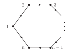
Figure 1: Null polygon in dual momentum superspace.

Here we present the basic Feynman rules for the proposed Wilson loop formulation of ${\cal N}=4$ amplitudes. We first consider a polygonal configuration given by $n$ points $(x_{i},\theta_{i})$ in ${\cal N}=4$ dual superspace [25], as shown in Figure 1. Adjacent points $i$ and $i+1$ are null separated, and we introduce dual momentum superspace coordinates,

$$x_{i}-x_{i+1}=p_{i}=\lambda_{i}\tilde{\lambda}_{i}~{},\qquad\theta_{i}-\theta_{i+1}=\lambda_{i}\eta_{i}~{},$$ (2.1)

with the conventions

$$x_{ab}=x_{a}-x_{b}~{},\qquad\theta_{ab}=\theta_{a}-\theta_{b}~{}.$$ (2.2)

We define the spinor $|\ell_{ab}\rangle_{\alpha}$ as

$$|\ell_{ab}\rangle\equiv|x_{ab}|\iota]~{},$$ (2.3)

where $|\iota]^{\dot{\alpha}}$ is an arbitrary reference spinor, as used in the MHV rules [2].

In Figure 2 we have summarized our diagrammatic rules in dual superspace or dual MHV rules for the calculation of tree and loop-level superamplitudes in ${\cal N}=4$ SYM. Note that the result is the superamplitude divided by the MHV tree-level superamplitude. We will illustrate these rules in detail in examples presented in later sections and will give here only some general comments.

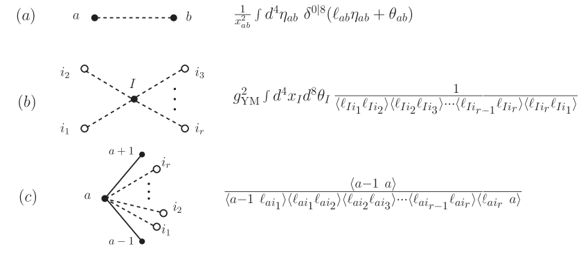
Figure 2: Feynman rules. (a) Propagator. (b) Internal vertices. (c) External vertices.

The propagator Figure 2(a) connects any pair of white dots from internal vertices, depicted in Figure 2(b), or external vertices, shown in Figure 2(c). A calculation of an $L$-loop superamplitude ${\cal A}_{{\rm N}^{k}{\rm MHV}}^{L\textrm{-loop}}$ would involve $k+L+1$ conventional spacetime MHV vertices. In the dual momentum picture, each internal vertex contributes a factor $g_{\rm YM}^{2}$ and fermionic degree $-8$, while each propagator contributes fermionic degree 4. Hence, in order to calculate ${\cal A}_{{\rm N}^{k}{\rm MHV}}^{L\textrm{-loop}}$, we need to sum over all possible diagrams with

$$\#({\rm internal\ vertices})=L~{},\qquad\#({\rm propagators})=k+2L~{}.$$ (2.4)

Before we move on to concrete tree and loop-level examples, we would like to make some general comments on the possible origin of these rules. The propagator resembles a standard scalar propagator, except for the presence of a fermionic integration. The internal vertices are most naturally interpreted as insertions arising from an MHV-type Lagrangian in dual momentum space, and finally, we expect the external vertices to arise from the expansion of an appropriate Wilson loop. In this respect we notice that two interesting proposals for Wilson loops in dual momentum space have recently appeared [22, 23], and it would be natural to expect that our rules are closely related to these. Finally, we note that our diagrammatic approach is, at least geometrically, a direct translation of the momentum twistor Wilson loop approach of [22], which makes the relation to supersymmetric MHV rules manifest.

3 Tree amplitudes

We begin by considering diagrams without internal vertices. As we shall see below, these turn out to generate the tree amplitudes of the ${\cal N}=4$ theory, divided by the tree MHV amplitude.

MHV tree amplitudes

In this case the number of propagators and internal vertices is zero. It can be viewed as a limiting case of the external vertex in Figure 2(c) with all dashed legs removed, to which we can assign the value $1$. This matches the MHV tree amplitude divided by itself.

NMHV tree amplitudes

The next simplest diagram without internal vertices is one with a single propagator linking two external vertices, labelled by $i$ and $j$ in Figure 3(a) below.

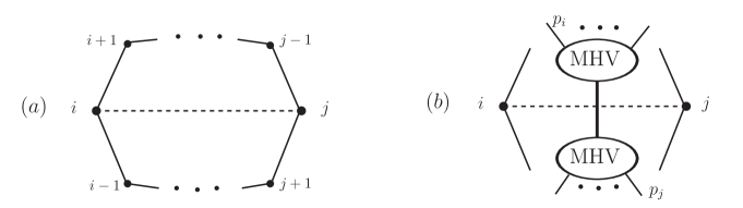
Figure 3: (a) Dual MHV diagrams contributing to NMHV tree amplitudes. (b) Here we show the conventional MHV diagrams together with the dual diagrams.

Applying our rules we obtain the expression

$${\langle i\!-\!1~{}i\rangle\over\langle i\!-\!1~{}\ell_{ij}\rangle\langle\ell_{ij}~{}i\rangle}{\langle j\!-\!1~{}j\rangle\over\langle j\!-\!1~{}\ell_{ij}\rangle\langle\ell_{ij}~{}j\rangle}{1\over x_{ij}^{2}}\int d^{4}\eta_{ij}~{}\delta^{0|8}(\ell_{ij}\eta_{ij}+\theta_{ij})~{}.$$ (3.1)

This is precisely the expression of the corresponding MHV diagram depicted in Figure 3(b), where we also show the dual momenta $x_{i}$ and $x_{j}$ in order to illustrate the graph duality between the two diagrams. Note that this term above is nothing but the superconformally invariant $R$-function [25] $R_{*;ij}=[*,i\!-\!1,i,j\!-\!1,j]$ in the notation of [30, 27] with reference twistor $Z_{*}=(0,\iota,0)$.

$\textrm{N}^{2}$MHV tree amplitudes

The next simplest dual MHV diagrams without internal vertices are depicted in Figure 4.

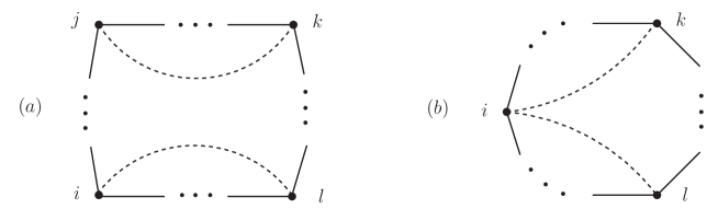
Figure 4: Dual MHV diagrams contributing to $\textrm{N}^{2}$MHV tree amplitudes. The corresponding ordinary MHV diagrams are depicted in Figure 5 below.

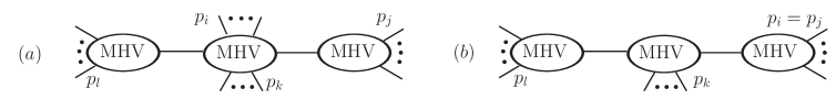
Figure 5: Conventional MHV diagrams for $\textrm{N}^{2}$MHV tree amplitudes.

These two kinds of diagrams will turn out to generate the ${\rm N}^{2}$MHV tree amplitude. The first one, given in Figure 4(a), gives

$${\langle i\!-\!1~{}i\rangle\over\langle i\!-\!1~{}\ell_{il}\rangle\langle\ell_{il}~{}i\rangle}{\langle l\!-\!1~{}l\rangle\over\langle l\!-\!1~{}\ell_{il}\rangle\langle\ell_{il}~{}l\rangle}{1\over x_{il}^{2}}\int d^{4}\eta_{il}~{}\delta^{0|8}(\ell_{il}\eta_{il}+\theta_{il})$$

$$\times{\langle j\!-\!1~{}j\rangle\over\langle j\!-\!1~{}\ell_{jk}\rangle\langle\ell_{jk}~{}j\rangle}{\langle k\!-\!1~{}k\rangle\over\langle k\!-\!1~{}\ell_{jk}\rangle\langle\ell_{jk}~{}k\rangle}{1\over x_{jk}^{2}}\int d^{4}\eta_{jk}~{}\delta^{0|8}(\ell_{jk}\eta_{jk}+\theta_{jk}).$$ (3.2)

The two lines in the expression above are independent as Figure 4(a) shows. This reproduces the result of conventional MHV diagram in Figure 5(a), divided by tree amplitude. The result is simply the product of two $R$-functions,

$$[*,j\!-\!1,j,k\!-\!1,k]\ [*,l\!-\!1,l,i\!-\!1,i].$$ (3.3)

The second type of diagrams contributing to the tree ${\rm N}^{2}$MHV amplitude is given in Figure 4(b), which corresponds to the special case $i=j$ of Figure 4(a). This gives

$${\langle i\!-\!1~{}i\rangle\over\langle i\!-\!1~{}\ell_{il}\rangle\langle\ell_{il}~{}\ell_{ik}\rangle\langle\ell_{ik}~{}i\rangle}{\langle k\!-\!1~{}k\rangle\over\langle k\!-\!1~{}\ell_{ik}\rangle\langle\ell_{ik}~{}k\rangle}{\langle l\!-\!1~{}l\rangle\over\langle l\!-\!1~{}\ell_{il}\rangle\langle\ell_{il}~{}l\rangle}$$

$$\times{1\over x_{il}^{2}}\int d^{4}\eta_{il}~{}\delta^{0|8}(\ell_{il}\eta_{il}+\theta_{il}){1\over x_{ik}^{2}}\int d^{4}\eta_{ik}~{}\delta^{0|8}(\ell_{ik}\eta_{ik}+\theta_{ik})\ .$$ (3.4)

It is readily seen that this is the same as the expression one obtains from the corresponding MHV diagram, in Figure 5(b). In the notation of [27], this diagram gives

$$[*,i\!-\!1,i,k\!-\!1,k]\ [*,\widehat{k\!-\!1},k,l\!-\!1,l],$$ (3.5)

where the hat refers to the shifting of the momentum twistor $\widehat{k\!-\!1}=(k\!-\!1,k)\cap(*,i\!-\!1,i)$. It is shown in [27] that the twistor expression (3.5) for this tree ${\rm N}^{2}$MHV amplitude matches that obtained from the MHV diagram approach, although this comparison is somewhat more involved than the one here.

Note that the multi-leg vertices (Figure 2(c) with $r\!>\!1$) make an appearance here with a vertex with $r\!=\!2$ being used, and that these vertices automatically take account of the special case that in the twistor picture requires the somewhat mysterious introduction of hatted twistor rules. We expect this to be a generic feature, i.e. that the “shifted twistors” of the rules of [27] will in general be automatic consequences of the Feynman rules proposed here.

Finally, we notice that there is a special class of dual MHV diagrams that apparently contributes to tree-level ${\rm N}^{2}$MHV superamplitudes, that is obtained by joining two external vertices with $r=2$ with two propagators, such as taking both $i=j$ and $k=l$ in Figure 4(a). Such a diagram, depicted in Figure 6, corresponds to a conventional MHV diagram with three vertices where the middle one would be bivalent, with its two legs connected to the adjacent MHV vertices. Due to the absence of conventional two-point MHV vertices, we expect such diagrams to vanish in the dual formulation, as we now check.

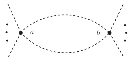
Figure 6: A dual MHV diagram potentially contributing to $\textrm{N}^{2}$MHV amplitudes which is not present in the conventional MHV diagram expansion. Its explicit contribution vanishes.

Denoting by $x_{a}$ and $x_{b}$ the positions of the external vertices in dual momentum space, we find this diagram to be equal to

$${\langle a\!-\!1~{}a\rangle\over\langle a\!-\!1~{}l_{ab}\rangle\langle l_{ab}~{}l_{ab}\rangle\langle l_{ab}~{}a\rangle}\,{\langle b\!-\!1~{}b\rangle\over\langle b\!-\!1~{}l_{ab}\rangle\langle l_{ab}~{}l_{ab}\rangle\langle l_{ab}~{}b\rangle}\,$$

$$\int\!d^{4}\eta_{ab}\,{\delta^{0|8}(\eta_{ab}l_{ab}+\theta_{ab})\over x_{ab}^{2}}\int\!d^{4}\eta_{ab}^{\prime}\,{\delta^{0|8}(\eta_{ab}^{\prime}l_{ab}+\theta_{ab})\over x_{ab}^{2}}\ .$$ (3.6)

The prefactor in (3) contains a double pole $1/\langle l_{ab}l_{ab}\rangle^{2}$. However, one has in general

$$\int\!d^{4}\eta d^{4}\eta^{\prime}\,\delta^{0|8}(\eta l+\theta)\delta^{0|8}(\eta^{\prime}l^{\prime}+\theta)\ =\ {1\over 16}\langle ll^{\prime}\rangle^{4}\prod_{A=1}^{4}\langle\theta^{A}\theta^{A}\rangle\ ,$$ (3.7)

and therefore the second line of (3) provides a factor of $\langle l_{ab}l_{ab}\rangle^{4}$. This compensates the double pole from the prefactor, and makes this class of diagrams vanish.

Generic tree amplitudes

It is clear from the examples discussed above that there is a direct correspondence between dual MHV diagrams without internal vertices, and tree-level MHV diagrams contributing to generic ${\rm N^{\it k}}$MHV amplitudes. This also covers all special cases where dual momenta coincide (c.f. Figure 4(b) above). This is the same diagrammatic duality discussed in Section 4.3 of [27], in the context of momentum twistor space.

4 One-loop amplitudes

In this section we start to consider loop amplitudes which requires us to include also internal vertices, represented in Figure 2(b), in the dual MHV diagrams. At one loop we thus have to consider dual MHV diagrams with one internal vertex.

One loop MHV amplitudes

The simplest Wilson loop with one internal vertex is given in Figure 7 below. Note that the dual superspace position $(x_{I},\theta_{I})$ of the internal vertex has to be integrated over. This diagram is equal to

$$g_{\rm YM}^{2}\int d^{4}x_{I}d^{8}\theta_{I}{1\over\langle\ell_{iI}\ell_{Ij}\rangle\langle\ell_{Ij}\ell_{iI}\rangle}\ {\langle i\!-\!1~{}i\rangle\over\langle i\!-\!1~{}\ell_{iI}\rangle\langle\ell_{iI}~{}i\rangle}{\langle j\!-\!1~{}j\rangle\over\langle j\!-\!1~{}\ell_{Ij}\rangle\langle\ell_{Ij}~{}j\rangle}$$

$${1\over x_{iI}^{2}}\int d^{4}\eta_{iI}~{}\delta^{0|8}(\ell_{iI}\eta_{iI}+\theta_{iI}){1\over x_{Ij}^{2}}\int d^{4}\eta_{Ij}~{}\delta^{0|8}(\ell_{Ij}\eta_{Ij}+\theta_{Ij})~{},$$ (4.1)

where the integration over the fermionic variables gives the factor $\langle\ell_{iI}\ell_{Ij}\rangle^{4}$. This yields exactly the result obtained from the one-loop MHV diagram in Figure 7(b) (divided by the tree amplitude).

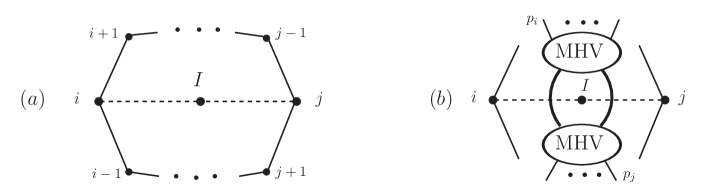
Figure 7: One-loop MHV amplitudes.

Generic one-loop amplitudes

Rather than reviewing the next simplest case, the one-loop NMHV amplitude, we consider instead the general structure of one-loop amplitudes in this formulation. The corresponding general structure in momentum twistor space has been discussed in Section 5.4 of [27]. By virtue of the tree-level results already obtained above, one may restrict the attention to diagrams containing one internal $n$-point vertex at $x_{I}$, whose legs connect to $m$ distinct points $x_{j_{r}}$ ($r=1,...,m$). The vertex generates a factor

$$g_{\rm YM}^{2}\int d^{4}x_{I}d^{8}\theta_{I}{1\over\langle\ell_{Ij_{1}}\ell_{Ij_{2}}\rangle\langle\ell_{Ij_{2}}\ell_{Ij_{3}}\rangle\cdots\langle\ell_{Ij_{m\!-\!1}}\ell_{Ij_{m}}\rangle\langle\ell_{Ij_{m}}\ell_{Ij_{1}}\rangle}~{}.$$ (4.2)

After performing the $\eta$ integrations coming from the propagators, each propagator connecting the internal vertex to the point $x_{j_{r}}$ generates a term,

$${1\over x_{Ij_{r}}^{2}}\delta^{0|4}(\langle\ell_{Ij_{r}}|\theta_{Ij_{r}}\rangle)~{}.$$ (4.3)

Finally, each external point $x_{j_{r}}$ with a propagator linked to it generates a term

$${\langle j_{r}\!-\!1\ j_{r}\rangle\over\langle j_{r}\!-\!1\ \ell_{Ij_{r}}\rangle\langle\ell_{Ij_{r}}\ j_{r}\rangle}.$$ (4.4)

Combining these three terms for all legs of the internal vertex one obtains the expression

$$g_{\rm YM}^{2}\prod_{r=1}^{m}\frac{\langle j_{r}\!-\!1\,j_{r}\rangle\ \delta^{0|4}(\langle\ell_{Ij_{r}}|\theta_{Ij_{r}}\rangle)}{x_{Ij_{r}}^{2}\,\langle j_{r}\!-\!1\,\ell_{Ij_{r}}\rangle\,\langle\ell_{Ij_{r}}\,j_{r}\rangle\,\langle\ell_{Ij_{r}}\,\ell_{Ij_{r\!+\!1}}\rangle}\,.$$ (4.5)

This is precisely the expression (5.22) of [27], obtained from the usual MHV rules and corresponds directly to the product of $R$ invariants that arises from applying the momentum twistor MHV rules discussed there. By this argument we see that the dual MHV rules proposed here correctly generate generic one-loop amplitudes as formulated by standard MHV diagrams.

5 Two loops

In this section we construct the integrand of the two-loop MHV amplitude from dual MHV rules. We will see that this integrand is the same as the standard integrand produced using spacetime MHV rules after dividing by the tree-level MHV amplitude. There are two main topologies of diagrams to consider, namely the double-bubble and the bubble-triangle topology, as shown in Figure 8. Special cases of such topologies arise when some of the external dual momenta coalesce.

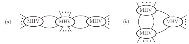
Figure 8: Two-loop MHV diagrams. (a) is the double-bubble, and (b) is the bubble-triangle.

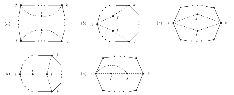
Figure 9: Two-loop MHV amplitudes. These graphs have two internal vertices and four propagators. Diagrams in the first line correspond to double-bubble MHV diagrams, and diagrams in the second line correspond to the bubble-triangle MHV diagrams.

In our description, we draw all possible diagrams that have two internal vertices and four propagators. The non-vanishing diagrams are shown in Figure 9. We consider them in turn.

Using the rules described in Section 2, we arrive at the following integrand for Figure 9(a):

$$g_{\rm YM}^{2}\int d^{4}x_{I}d^{8}\theta_{I}{1\over\langle\ell_{Ii}\ell_{Il}\rangle^{2}}\,g_{\rm YM}^{2}\int d^{4}x_{J}d^{8}\theta_{J}{1\over\langle\ell_{Jj}\ell_{Jk}\rangle^{2}}$$

$${1\over x_{iI}^{2}}\int d^{4}\eta_{iI}~{}\delta^{0|8}(\ell_{iI}\eta_{iI}+\theta_{iI}){1\over x_{Il}^{2}}\int d^{4}\eta_{Il}~{}\delta^{0|8}(\ell_{Il}\eta_{Il}+\theta_{Il})$$

$${1\over x_{jJ}^{2}}\int d^{4}\eta_{jJ}~{}\delta^{0|8}(\ell_{jJ}\eta_{jJ}+\theta_{jJ}){1\over x_{Jk}^{2}}\int d^{4}\eta_{Jk}~{}\delta^{0|8}(\ell_{Jk}\eta_{Jk}+\theta_{Jk})$$

$${\langle i\!-\!1\,i\rangle\over\langle i\!-\!1\,\ell_{Ii}\rangle\langle\ell_{Ii}\,i\rangle}\,{\langle j\!-\!1\,j\rangle\over\langle j\!-\!1\,\ell_{jJ}\rangle\langle\ell_{jJ}\,j\rangle}\,{\langle k\!-\!1\,k\rangle\over\langle k\!-\!1\,\ell_{Jk}\rangle\langle\ell_{Jk}\,k\rangle}\,{\langle l\!-\!1\,l\rangle\over\langle l\!-\!1\,\ell_{lI}\rangle\langle\ell_{lI}\,l\rangle}\ .$$ (5.1)

The first line in (5) corresponds to the insertion of two internal two-point vertices, the second and third line to four propagators connecting the two-point vertices with four external vertices, appearing in the last line, located at dual points $x_{i}$, $x_{j}$, and $x_{k}$, $x_{m}$. The fermionic integrations can be performed immediately, and give $\langle\ell_{iI}\ell_{lI}\rangle^{4}\langle\ell_{jJ}\ell_{kJ}\rangle^{4}$. After this, (5) is immediately found to coincide with the integrand of the corresponding spacetime two-loop MHV diagram.

Next we consider the class of diagrams where $x_{i}=x_{j}$, corresponding to Figure 9(b). These are given by

$$g_{\rm YM}^{2}\int d^{4}x_{I}d^{8}\theta_{I}{1\over\langle\ell_{Ii}\ell_{Il}\rangle^{2}}\,g_{\rm YM}^{2}\int d^{4}x_{J}d^{8}\theta_{J}{1\over\langle\ell_{Ji}\ell_{Jk}\rangle^{2}}$$

$${1\over x_{iI}^{2}}\int d^{4}\eta_{iI}~{}\delta^{0|8}(\ell_{iI}\eta_{iI}+\theta_{iI}){1\over x_{Il}^{2}}\int d^{4}\eta_{Il}~{}\delta^{0|8}(\ell_{Il}\eta_{Il}+\theta_{Il})$$

$${1\over x_{iJ}^{2}}\int d^{4}\eta_{iJ}~{}\delta^{0|8}(\ell_{iJ}\eta_{iJ}+\theta_{iJ}){1\over x_{Jk}^{2}}\int d^{4}\eta_{Jk}~{}\delta^{0|8}(\ell_{Jk}\eta_{Jk}+\theta_{Jk})$$

$${\langle i\!-\!1\,i\rangle\over\langle i\!-\!1\,\ell_{Ii}\rangle\langle\ell_{Ii}\,\ell_{iJ}\rangle\langle\ell_{iJ}\,i\rangle}\,{\langle k\!-\!1\,k\rangle\over\langle k\!-\!1\,\ell_{kJ}\rangle\langle\ell_{kJ}\,k\rangle}\,{\langle l\!-\!1\,l\rangle\over\langle l\!-\!1\,\ell_{lI}\rangle\langle\ell_{lI}\,l\rangle}\ .$$ (5.2)

Compared to (5), we notice the appearance in the fourth line of (5) of an external vertex with $r=2$ – see Figure 2(c). Once again fermionic integrations are trivial to perform and give $\langle\ell_{iI}\ell_{lI}\rangle^{4}\langle\ell_{iJ}\ell_{kJ}\rangle^{4}$, and one then recognises instantly that (5) is equal to the corresponding spacetime MHV diagram.

There is an additional case with the same double-bubble topology, where the middle MHV vertex has no external legs – it is only attached to two adjacent MHV vertices forming the two loops of the diagram. This correspond to Figure 9(c), and is also immediately seen to reproduce the corresponding spacetime MHV result.

The last diagram topology to consider is the triangle-bubble. In the most general of diagrams, one has an internal three-point and an internal two-point vertex, connected together by propagators and connected to external vertices given in Figure 2(c) (with $r\!=\!1$, in the notation of the Figure). The diagram is depicted in Figure 9(d) and equals

$$g_{\rm YM}^{2}\int d^{4}x_{I}d^{8}\theta_{I}{1\over\langle\ell_{Ii}\ell_{IJ}\rangle^{2}}\,g_{\rm YM}^{2}\int d^{4}x_{J}d^{8}\theta_{J}{1\over\langle\ell_{IJ}\ell_{Jj}\rangle\langle\ell_{Jj}\ell_{Jk}\rangle\ell_{Jk}\ell_{IJ}\rangle}$$

$${1\over x_{iI}^{2}}\int d^{4}\eta_{iI}~{}\delta^{0|8}(\ell_{iI}\eta_{iI}+\theta_{iI}){1\over x_{IJ}^{2}}\int d^{4}\eta_{IJ}~{}\delta^{0|8}(\ell_{IJ}\eta_{IJ}+\theta_{IJ})$$

$${1\over x_{Jj}^{2}}\int d^{4}\eta_{Jj}~{}\delta^{0|8}(\ell_{Jj}\eta_{Jj}+\theta_{Jj}){1\over x_{kJ}^{2}}\int d^{4}\eta_{kJ}~{}\delta^{0|8}(\ell_{kJ}\eta_{kJ}+\theta_{kJ})$$

$${\langle i\!-\!1\,i\rangle\over\langle i\!-\!1\,\ell_{Ii}\rangle\langle\ell_{Ii}\,i\rangle}\,{\langle j\!-\!1\,j\rangle\over\langle j\!-\!1\,\ell_{jJ}\rangle\langle\ell_{jJ}\,j\rangle}\,{\langle k\!-\!1\,k\rangle\over\langle k\!-\!1\,\ell_{kJ}\rangle\langle\ell_{kJ}\,k\rangle}\ .$$ (5.3)

A special case occurs when $i=j$ as shown in Figure 9(e), which is also immediately seen to reproduce the corresponding spacetime MHV result.

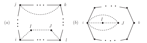
Figure 10: These diagrams give zero contribution.

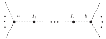
Figure 11: The diagram which contains a chain of two-point vertices ($r>1$) also gives a vanishing contribution.

There are other graphs, shown in Figure 10, but they all give vanishing contribution. For example, when there is a structure of a chain of internal two-point vertices, as in Figure 11, the result is zero. Indeed, considering only the fermionic part, we have

$$\int d^{8}\theta_{I_{1}}\cdots\theta_{I_{r}}d^{4}\eta_{aI_{1}}\cdots d^{4}\eta_{I_{r}b}~{}\delta^{0|8}(\ell_{aI_{1}}\eta_{aI_{1}}+\theta_{aI_{1}})\cdots\delta^{0|8}(\ell_{I_{r}b}\eta_{I_{r}b}+\theta_{I_{r}b})$$ (5.4)

$$= \int d^{4}\eta_{aI_{1}}\cdots d^{4}\eta_{I_{r}b}~{}\delta^{0|8}(\ell_{aI_{1}}\eta_{aI_{1}}+\cdots+\ell_{I_{r}b}\eta_{I_{r}b}+\theta_{ab})~{},$$

and unless $r=1$ the integration always gives zero. This is what happens for Figure 10(a). Figure 10(b) contains the structure made by joining two internal two-point vertices with two propagators, which also vanishes as discussed in section 3.

6 Discussion

The proposal given here provides a MHV diagram formulation of all ${\cal N}=4$ amplitudes in dual momentum space, which is dual to the conventional MHV diagram approach [2]. This is the dual momentum version (i.e. dual space-time version) of the momentum twistor space Wilson loop approach of [22]. Whilst one may appeal to that formulation to argue that the Feynman rules given here must necessarily arise from the ${\cal N}=4$ theory, there is presumably a direct argument for this. The internal vertices of Figure 2(b) appear to be of MHV origin, and together with the kinetic terms giving the propagator of Figure 2(a) may be related to the ${\cal N}=4$ formulation of [8, 9]. As discussed in Section 2, the external vertices of Figure 2(c) should then arise from the definition of a Wilson loop, perhaps along the lines of the twistor space argument presented in [22]. It would also be interesting to relate the rules here to some lightcone limit of correlation functions, along the lines of recent work [31, 32, 33] (see also [23]).

There are some interesting features of the Feynman rules in Figure 2 that may throw light on these. We note that the external vertices are inserted at points in dual momentum space, with the simplest insertion corresponding to adding one soft function, and $n$-point insertions corresponding to a multiple soft function with $n$ legs becoming soft. Multiplying by soft functions is the natural way to add particles in the Yangian symmetric [34] formalism of [21, 35], and this may bear further examination. These multiple field insertions in the external vertices are relevant when some dual momentum regions coalesce, and the corresponding rules are very simple modifications of those for less exceptional cases. Their origin should come from the expansion of a dual momentum Wilson loop. The fact that the rules presented here appear to automatically take account of shifted twistors in [22] also supports this.

Finally, we notice that collinear and multi-particle singularities of the dual MHV diagrams correspond to dual momenta becoming lightlike separated, and may therefore be obtained by a lightcone operator product expansion. It would also be interesting to relate this to recent work of [36].

References

- [1] E. Witten, Perturbative gauge theory as a string theory in twistor space, Commun. Math. Phys. 252 (2004) 189 [arXiv:hep-th/0312171].
- [2] F. Cachazo, P. Svrcek and E. Witten, MHV vertices and tree amplitudes in gauge theory, JHEP 0409 (2004) 006 [arXiv:hep-th/0403047].
- [3] A. Brandhuber, B. J. Spence and G. Travaglini, One-loop gauge theory amplitudes in N = 4 super Yang-Mills from MHV vertices, Nucl. Phys. B 706 (2005) 150 [arXiv:hep-th/0407214].
- [4] A. Brandhuber, B. Spence and G. Travaglini, From trees to loops and back, JHEP 0601 (2006) 142 [arXiv:hep-th/0510253].
- [5] J. Bedford, A. Brandhuber, B. J. Spence and G. Travaglini, A twistor approach to one-loop amplitudes in N = 1 supersymmetric Yang-Mills theory, Nucl. Phys. B 706 (2005) 100 [arXiv:hep-th/0410280].
- [6] C. Quigley and M. Rozali, One-loop MHV amplitudes in supersymmetric gauge theories, JHEP 0501, 053 (2005) [arXiv:hep-th/0410278].
- [7] J. Bedford, A. Brandhuber, B. J. Spence and G. Travaglini, Non-supersymmetric loop amplitudes and MHV vertices, Nucl. Phys. B 712 (2005) 59 [arXiv:hep-th/0412108].
- [8] A. Gorsky and A. Rosly, From Yang-Mills Lagrangian to MHV diagrams, JHEP 0601 (2006) 101 [arXiv:hep-th/0510111].
- [9] P. Mansfield, The Lagrangian origin of MHV rules, JHEP 0603 (2006) 037 [arXiv:hep-th/0511264].
- [10] R. Boels, L. Mason and D. Skinner, Supersymmetric gauge theories in twistor space, JHEP 0702, 014 (2007) [arXiv:hep-th/0604040].
- [11] R. Boels, L. Mason and D. Skinner, From Twistor Actions to MHV Diagrams, Phys. Lett. B 648, 90 (2007) [arXiv:hep-th/0702035].
- [12] L. F. Alday and J. Maldacena, Gluon scattering amplitudes at strong coupling, JHEP 0706 (2007) 064 [arXiv:0705.0303 [hep-th]].
- [13] G. P. Korchemsky, J. M. Drummond and E. Sokatchev, Conformal properties of four-gluon planar amplitudes and Wilson loops, Nucl. Phys. B 795, 385 (2008) [arXiv:0707.0243 [hep-th]].
- [14] A. Brandhuber, P. Heslop and G. Travaglini, MHV Amplitudes in N=4 Super Yang-Mills and Wilson Loops, Nucl. Phys. B 794, 231 (2008) [arXiv:0707.1153 [hep-th]].
- [15] J. M. Drummond, J. Henn, G. P. Korchemsky and E. Sokatchev, On planar gluon amplitudes/Wilson loops duality, Nucl. Phys. B 795, 52 (2008) [arXiv:0709.2368 [hep-th]].
- [16] J. M. Drummond, J. Henn, G. P. Korchemsky and E. Sokatchev, Conformal Ward identities for Wilson loops and a test of the duality with gluon amplitudes, Nucl. Phys. B 826, 337 (2010) [arXiv:0712.1223 [hep-th]].
- [17] Z. Bern, L. J. Dixon, D. A. Kosower, R. Roiban, M. Spradlin, C. Vergu and A. Volovich, The Two-Loop Six-Gluon MHV Amplitude in Maximally Supersymmetric Yang-Mills Theory, Phys. Rev. D 78, 045007 (2008) [arXiv:0803.1465 [hep-th]].
- [18] J. M. Drummond, J. Henn, G. P. Korchemsky and E. Sokatchev, Hexagon Wilson loop = six-gluon MHV amplitude, Nucl. Phys. B 815, 142 (2009) [arXiv:0803.1466 [hep-th]].
- [19] C. Anastasiou, A. Brandhuber, P. Heslop, V. V. Khoze, B. Spence and G. Travaglini, Two-Loop Polygon Wilson Loops in N=4 SYM, JHEP 0905, 115 (2009) [arXiv:0902.2245 [hep-th]].
- [20] C. Vergu, The two-loop MHV amplitudes in N=4 supersymmetric Yang-Mills theory, arXiv:0908.2394 [hep-th].
- [21] N. Arkani-Hamed, J. L. Bourjaily, F. Cachazo, S. Caron-Huot and J. Trnka, The All-Loop Integrand For Scattering Amplitudes in Planar N=4 SYM, arXiv:1008.2958 [hep-th].
- [22] L. Mason and D. Skinner, The Complete Planar S-matrix of N=4 SYM as a Wilson Loop in Twistor Space, arXiv:1009.2225 [hep-th].
- [23] S. Caron-Huot, Notes on the scattering amplitude / Wilson loop duality, arXiv:1010.1167 [hep-th].
- [24] J. M. Drummond, J. Henn, V. A. Smirnov and E. Sokatchev, Magic identities for conformal four-point integrals, JHEP 0701, 064 (2007) [arXiv:hep-th/0607160].
- [25] J. M. Drummond, J. Henn, G. P. Korchemsky and E. Sokatchev, Dual superconformal symmetry of scattering amplitudes in N=4 super-Yang-Mills theory, Nucl. Phys. B 828, 317 (2010) [arXiv:0807.1095 [hep-th]].
- [26] A. Hodges, Eliminating spurious poles from gauge-theoretic amplitudes, arXiv:0905.1473 [hep-th].
- [27] M. Bullimore, L. Mason and D. Skinner, MHV Diagrams in Momentum Twistor Space, arXiv:1009.1854 [hep-th].
- [28] G. Georgiou and V. V. Khoze, Tree amplitudes in gauge theory as scalar MHV diagrams, JHEP 0405 (2004) 070 [arXiv:hep-th/0404072].
- [29] G. Georgiou, E. W. N. Glover and V. V. Khoze, Non-MHV Tree Amplitudes in Gauge Theory, JHEP 0407 (2004) 048 [arXiv:hep-th/0407027].
- [30] L. Mason and D. Skinner, Dual Superconformal Invariance, Momentum Twistors and Grassmannians, JHEP 0911 (2009) 045, 0909.0250 [hep-th]].
- [31] L. F. Alday, B. Eden, G. P. Korchemsky, J. Maldacena and E. Sokatchev, From correlation functions to Wilson loops, arXiv:1007.3243 [hep-th].
- [32] B. Eden, G. P. Korchemsky and E. Sokatchev, From correlation functions to scattering amplitudes, arXiv:1007.3246 [hep-th].
- [33] B. Eden, G. P. Korchemsky and E. Sokatchev, More on the duality correlators/amplitudes, arXiv:1009.2488 [hep-th].
- [34] J. M. Drummond, J. M. Henn and J. Plefka, Yangian symmetry of scattering amplitudes in N=4 super Yang-Mills theory, JHEP 0905 (2009) 046 [arXiv:0902.2987 [hep-th]].
- [35] N. Arkani-Hamed, F. Cachazo, C. Cheung and J. Kaplan, A Duality For The S Matrix, JHEP 1003 (2010) 020 [arXiv:0907.5418 [hep-th]].
- [36] L. F. Alday, D. Gaiotto, J. Maldacena, A. Sever and P. Vieira, An Operator Product Expansion for Polygonal null Wilson Loops, arXiv:1006.2788 [hep-th].