Geometry and Statistics of Ehrenfest dynamics

Abstract

Quantum dynamics (e.g., the Schrödinger equation) and classical dynamics (e.g., Hamilton equations) can both be formulated in equal geometric terms: a Poisson bracket defined on a manifold. The difference between both worlds is due to the presence of extra structure in the quantum case, that leads to the appearance of the probabilistic nature of the measurements and the indetermination and superposition principles. In this paper we first show that the quantum-classical dynamics prescribed by the Ehrenfest equations can also be formulated within this general framework, what has been used in the literature to construct propagation schemes for Ehrenfest dynamics. Then, the existence of a well defined Poisson bracket allows to arrive to a Liouville equation for a statistical ensemble of Ehrenfest systems. The study of a generic toy model shows that the evolution produced by Ehrenfest dynamics is ergodic and therefore the only constants of motion are functions of the Hamiltonian. The emergence of the canonical ensemble characterized by the Boltzmann’s distribution follows after an appropriate application of the principle of equal a priori probabilities to this case. This work provides the basis for extending stochastic methods to Ehrenfest dynamics.

I Introduction

There is little doubt that the solution of Schrödinger equation for a combined system of electrons and nuclei enables us to predict most of the chemistry and molecular physics that surrounds us, including bio-physical processes of great complexity. Yet there is also little doubt that this task is not possible in general, and approximations need to be made; one of the most important and successful being the classical approximation for a number of the particles. Mixed quantum-classical dynamical (MQCD) models are therefore necessary and widely used.

The so-called “Ehrenfest equations” (EE) result from a straightforward application of the classical limit to a portion of the particles of a full quantum system, and constitute the most evident MQCD model, as well as a first step in the intricated problem of mixing quantum and classical dynamics. For example, it can be noted that much of the field of molecular dynamics (MD) – whether ab initio or not – is based on equations that can be obtained from further approximations to the Ehrenfest model: for instance, written in the adiabatic basis, the Ehrenfest dynamics collapse into Born Oppenheimer MD if we assume the non-adiabatic couplings to be negligible.

It is not the purpose of this work, however, to dwell into the justification or validity conditions of the EE (see for example Refs. Marx and Hutter, 2009; Gerber et al., 1982; Gerber and Ratner, 1988; Bornemann et al., 1996, 1995 for rigurous analyses). Nor is it to investigate the unsettled problem of which is the best manner of mixing quantum and classical degrees of freedom. The Ehrenfest model has a proven application niche, and for this reason we are interested in investigating some of its theoretical foundations, in a manner and with an aim that we describe in the following. 

Classical mechanics (CM) can be formulated in several mathematical frameworks, each corresponding to a different level of abstraction (Newton’s equations, the Hamiltonian formalism, the Poisson brackets, etc.). Perhaps its more abstract and general formulation is geometrical, in terms of Poisson manifolds. Similarly, quantum mechanics (QM) can be formulated in different ways, some of which resemble its classical counterpart. For example, the observables (self-adjoint linear operators) are endowed with a Poisson algebra almost equal to the one that characterizes the dynamical variables in CM. Moreover, Schrödinger equation can be recast into Hamiltonian equations form Heslot (1985) by transforming the complex Hilbert space into a real one of double dimension; the observables are also transformed into dynamical functions in this new phase space, in analogy with the classical case. Finally, a Poisson bracket formulation has also been established for QM, which permits to classify both the classical and the quantum dynamics under the same heading.

This variety of formulations does not emerge from academic caprice; the successive abstractions simplify further developments of the theory, such as the step from microscopic dynamics to statistical dynamics: the derivation of Liouville’s equation (or von Neumann’s equation in the quantum case), at the heart of statistical dynamics, is based on the properties of the Poisson algebra.

The issue regarding what is the correct equilibrium distribution of a mixed quantum-classical system is seen as a very relevant one. Parandekar and Tully (2006); Käb (2006); Bastida et al. (2006); Käb (2002); Tully (1998); Müller and Stock (1997); Mauri et al. (1993); Terashima et al. (2001) An attempt to its derivation can be found in Ref. Mauri et al., 1993, where they arrive to the same distribution that we will advocate below, although it is done using the Nosé-Hoover technique,Nosé (1984, 1991) which is only a mathematical scheme to produce the equilibrium, and which the very authors of Ref. Mauri et al., 1993 agree that it is not clear how to apply to a mixed quantum-classical dynamics. In Ref. Parandekar and Tully, 2006 they provide some analytical results about this distribution, but not in the case in which the system of interest is described by the EE; instead (and as in Refs. Käb, 2006; Bastida et al., 2006), they assume that the system is fully quantum, and that it is coupled to an infinite classical bath via an Ehrenfest-like interaction.

It is therefore necessary to base Ehrenfest dynamics – or any other MQCD model – on firm theoretical ground. In particular, we are interested in establishing a clear path to statistical mechanics for Ehrenfest systems, which in our opinion should be done by first embedding this dynamics into the same theoretical framework used in the pure classical or quantum cases (i.e., Poisson brackets, symplectic forms, etc). Then the study of their statistics will follow the usual steps for purely classical or purely quantum ensembles. In this respect, it should be noted that other approaches to MQCD (not based on Ehrenfest equations) exist,Kisil (1996); Prezhdo and Kisil (1997); Kapral and Ciccotti (1999) and to their corresponding statistics; Nielsen et al. (2001); Kapral (2001) however it has been found that the formulation of well defined quantum-classical brackets (i.e., satisfying the Jacobi identity and Leibniz derivation rule) is a difficult issue. Kisil (2005); Agostini et al. (2007); Kisil (2010); Agostini et al. (2010) On the contrary, as shown below, and as a result of the fact that the evolution of a quantum system can be formulated in terms of Hamilton equations similar to those of a classical system,Bornemann et al. (1996); Schmitt and Brickmann (1996) we will not have difficulties in a rigorous formulation of the Ehrenfest dynamics in terms of Poisson brackets.

The roadmap of this project is the following: In Section II we recall the definition of the Ehrenfest model. In Section III we summarize quickly the formulation of CM in terms of Poisson brackets. Then we summarize, in Section IV, the analogous description of QM in terms of geometrical objects which can be found, for example, in Refs. Kibble, 1979; Heslot, 1985; Abbati et al., 1984; Cirelli et al., 1991; Brody and Hughston, 2001; Ashtekar and Schilling, 1998; Cariñena et al., 2006, 2007; Clemente-Gallardo and Marmo, 2008. These works demonstrate how Schrödinger equation can be written as a set of (apparently classical) Hamiltonian equations. Also, by using a suitable definition of observables as functions on the (real) set of physical states, Schrödinger equation can be written in terms of a canonical Poisson bracket. QM appears in this way as “classical”, although the existence of extra algebraic structure encodes the probabilistic interpretation of measurements, and the superposition and indetermination principles Kibble (1979); Abbati et al. (1984); Cirelli et al. (1991); Brody and Hughston (2001); Ashtekar and Schilling (1998) . For the case of Ehrenfest dynamics, we can now combine it (Section V) with CM, whose Poisson bracket formulation is very well known. The procedure is very simple: we consider as a global phase space the Cartesian product of the electronic and the nuclear phase spaces and define a global Poisson bracket simply as the sum of the classical and the quantum ones. It is completely straightforward to prove that such a Poisson bracket is well defined and that it provides the correct dynamical equations (EE).

From a formal point of view, the resulting dynamics is more similar to a classical system than to a quantum one, although when considering a pure quantum system the dynamics is the usual Schrödinger one. This is not surprising since the coupling of the classical and quantum systems makes the total system nonlinear in its evolution, and this is one of the most remarkable differences between a classical and a quantum system in any formulation.

Once the dynamical description as a Poisson system is at our disposal, it is a very simple task (Section VI) to construct the corresponding statistical description following the lines of Refs. Balescu, 1997 and Balescu, 1975. The formal similarity with the CM case ensures the correctness of the procedure and allows us to derive a Liouville equation. The choice of the equilibrium distribution is based, as usual, in the principle of equal a priori probablities implicitely used by Gibbs and clearly formulated by Tolman Tolman (1938).

Finally, in the conclusions (Section VII), we propose to extend, within our formalism, stochastic methods to Ehrenfest dynamics.

II The Ehrenfest model

The Ehrenfest Equations have the following general form:

$$\dot{\vec{R}}_{J}(t) = \langle\psi(t)|\frac{\partial\hat{H}}{\partial\vec{P}_{J}}(\vec{R}(t),\vec{P}(t),t)|\psi(t)\rangle,$$ (1)

$$\dot{\vec{P}}_{J}(t) = -\langle\psi(t)|\frac{\partial\hat{H}}{\partial\vec{R}_{J}}(\vec{R}(t),\vec{P}(t),t)|\psi(t)\rangle,$$ (2)

$$i\hbar\frac{{\rm d}}{{\rm d}t}|\psi(t)\rangle = \hat{H}(\vec{R}(t),\vec{P}(t),t)|\psi(t)\rangle,$$ (3)

where $(\vec{R},\vec{P})$ denote collectively the set of canonical position and momenta coordinates of a set of classical particles, whereas $\psi$ is the wavefunction of the quantum part of the system. See Ref  Andrade et al., 2009 for the issue of the Hellmann-Feynman theorem in this context – i.e., whether one should take the derivative inside or outside the expectation value.

This and other MQCD models appear in different contexts; in many situations, the division into quantum and classical particles is made after the electrons have been integrated out, and is used to quantize a few of the nuclear degrees of freedom. However, a very obvious case to use EE is when we want to treat electrons quantum mechanically, and nuclei classically. In order to fix ideas, let us use this case as an example: the Hamiltonian for the full quantum system is:

$$\hat{H}= -\hbar^{2}\sum_{J}\frac{1}{2M_{J}}\nabla_{J}^{2}-\hbar^{2}\sum_{j}\frac{1}{2}\nabla_{j}^{2}+\frac{1}{4\pi\epsilon_{0}}\sum_{J<K}\frac{Z_{J}Z_{K}}{|\vec{R}_{J}-\vec{R}_{K}|}$$

$$-\frac{1}{4\pi\epsilon_{0}}\sum_{j<k}\frac{1}{|\vec{r}_{j}-\vec{r}_{k}|}-\frac{1}{4\pi\epsilon_{0}}\sum_{J,j}\frac{Z_{J}}{|\vec{R}_{J}-\vec{r}_{j}|}$$

$$= -\hbar^{2}\sum_{J}\frac{1}{2M_{J}}\nabla_{J}^{2}-\hbar^{2}\sum_{j}\frac{1}{2}\nabla_{j}^{2}+V_{n-e}(\vec{r},\vec{R})$$

$$= -\hbar^{2}\sum_{J}\frac{1}{2M_{J}}\nabla_{J}^{2}+H_{e}(\vec{r},\vec{R}),$$ (4)

where all sums must be understood as running over the whole natural set for each index. $M_{J}$ is the mass of the J-th nucleus in units of the electron mass, and $Z_{J}$ is the charge of the J-th nucleus in units of (minus) the electron charge. Also note that we have defined the nuclei-electrons potential $V_{n-e}(\vec{r},\vec{R})$ and the electronic Hamiltonian $H_{e}(\vec{r},\vec{R})$ operators.

The EE may then be reached in the following way:Marx and Hutter (2009); Gerber et al. (1982); Gerber and Ratner (1988); Bornemann et al. (1996, 1995) first, the full wave function is split into a product of nuclear and electronic wave functions, which leads to the time dependent self-consistent field model, in which the two subsystems are quantum and coupled. Afterwards, a classical limit procedure is applied to the nuclear subsystem, and the EE emerge naturally. In terms of the nuclei positions $\vec{R}_{J}$ and of the element of the Hilbert space $|\psi\rangle\in\mathcal{H}$ which encodes the state of the electrons of the system, the Ehrenfest dynamics is then given by

$$M_{J}\ddot{\vec{R}}_{J} =-\langle\psi|\nabla_{J}H_{e}(\vec{r},\vec{R})|\psi\rangle,$$ (5)

$$i\hbar\frac{d}{dt}|\psi\rangle =H_{e}(\vec{r},\vec{R})|\psi\rangle.$$ (6)

These equations can be given a Hamiltonian-type description by introducing a Hamiltonian function of the form:

$$H(\vec{R},\vec{P})=\sum_{J}\frac{\vec{P}_{J}^{2}}{2M_{J}}+\langle\psi|H_{e}(\vec{r},\vec{R})|\psi\rangle.$$ (7)

Then, by fixing a relation of the form $\vec{P}_{J}=M\dot{\vec{R}}_{J}$, we obtain a structure similar to Hamilton equations:

$$\dot{\vec{R}}_{J} =\frac{\vec{P}_{J}}{M_{J}},$$ (8)

$$\dot{\vec{P}}_{J} =-\langle\psi|\nabla_{J}H_{e}(\vec{r},\vec{R})|\psi\rangle,$$ (9)

$$i\hbar\frac{d}{dt}|\psi\rangle =H_{e}(\vec{r},\vec{R})|\psi\rangle.$$ (10)

But in spite of the formal similarities, these equations do not correspond yet to Hamilton equations, since they lack a global phase space formulation (encompassing both the nuclear and the electronic degrees of freedom) and a Poisson bracket.

III Classical mechanics in terms of Poisson brackets

Let us begin by recalling very quickly the Hamiltonian formulation of classical dynamics. We address the interested reader to a classical text, such as Ref. Abraham and Marsden, 1978, for a more detailed presentation.

Let us consider a classical system with phase space $M_{C}$, which, for the sake of simplicity, we can identify with $\mathbb{R}^{2n}$, where $n$ is the number of degrees of freedom (strictly speaking, $M_{C}$ is a general $2n$-dimensional manifold, homeomorphic to $\mathbb{R}^{2n}$ only locally). The $2n$ dimensions correspond with the $n$ position coordinates that specify the configuration of the system, and the $n$ corresponding momenta (mathematically, however, the division into “position” and “momenta” coordinates is a consequence of Darboux theorem – see below).

In what regards the observables, classical mechanics uses the set of differentiable functions

$$f:M_{C}\to\mathbb{R},$$ (11)

assigning the result of the measurement to every point in $M_{C}$. On this set of functions $C^{\infty}(M_{C})$ we introduce an operation, known as Poisson bracket, which allows us to study the effect of symmetry transformations and also the dynamical evolution. The precise definition is as follows:

Definition 1

A Poisson bracket, $\{\cdot,\cdot\}$, is a bilinear operation

$$\{\cdot,\cdot\}:C^{\infty}(M_{C})\times C^{\infty}(M_{C})\to C^{\infty}(M_{C}),$$ (12)

which:

• It is antisymmetric,

  $$\{f,g\}=-\{g,f\},\qquad\forall f,g\in C^{\infty}(M_{C}).$$

• It satisfies the Jacobi identity, i.e., $\forall f,g,h\in C^{\infty}(M_{C})$:

  $$\{f,\{g,h\}\}+\{h,\{f,g\}\}+\{g,\{h,f\}\}=0.$$

• It satisfies the Leibniz rule ,i.e., $\forall f,g,h\in C^{\infty}(M_{C})$:

  $$\{f,gh\}=\{f,g\}h+g\{f,h\}.$$

A Poisson bracket allows us also to introduce the concept of Hamiltonian vector field:

Definition 2

Given a function $f\in C^{\infty}(M_{C})$ and a Poisson bracket $\{\cdot,\cdot\}$, a vector field, $X_{f}$, is said to be its Hamiltonian vector field if

$$X_{f}(g)=\{f,g\},\qquad\forall g\in C^{\infty}(M_{C}).$$

Definition 3

We shall call a Hamiltonian system to a triple $(M_{C},\{\cdot,\cdot\},H)$, where $\{\cdot,\cdot\}$ is a Poisson bracket on $M_{C}$, and dynamics is introduced via the function $H\in C^{\infty}(M_{C})$, that we call the Hamiltonian.

If the Poisson bracket is non degenerate (it has no Casimir functions), a theorem due to Darboux ensures that there exists a set of coordinates $(\vec{R},\vec{P})$ for which the bracket has the “standard” form (at least locally, in a neighbourhood of every point):

$$\{f_{1},f_{2}\}=\sum_{k=1}^{n}\frac{\partial f_{1}}{\partial P_{k}}\frac{\partial f_{2}}{\partial R^{k}}-\frac{\partial f_{1}}{\partial R^{k}}\frac{\partial f_{2}}{\partial P_{k}}.$$ (13)

These coordinates are called Darboux coordinates. They are specially useful when studying the dynamics and invariant measures of a Hamiltonian systemAbraham and Marsden (1978). In the rest of the paper we shall be working with this kind of coordinates.

Then, given $f\in C^{\infty}(\mathbb{R}^{2n})$, we can write the corresponding Hamiltonian vector field $X_{f}$ as

$$X_{f}=\sum_{k=1}^{n}\frac{\partial f(R,P)}{\partial P_{k}}\frac{\partial}{\partial R^{k}}-\frac{\partial f(R,P)}{\partial R^{k}}\frac{\partial}{\partial P_{k}}.$$ (14)

Now one can consider two different formulations of the dynamics:

• One which defines the corresponding Hamiltonian vector field $X_{H}$ obtained as above

  $$X_{H}(g)=\{H,g\},\qquad\forall g\in C^{\infty}(M_{C}).$$

  The integral curves of the vector field $X_{H}$ define the solution of the dynamics.

• An analogous formulation can be given in terms of the observables. If we consider now the set of functions of the system, i.e., the set of classical observables, the dynamics is written as the Poisson bracket of the Hamiltonian function $H$ with any other function of the system, i.e.,

  $$\frac{df}{dt}=\{H,f\},\qquad\forall f\in C^{\infty}(M_{C}).$$ (15)

Both approaches are equivalent: the differential equations that determine the integral curves of the Hamiltonian vector field are given by Eq. 15, for the functions “position” and “momenta” of each particle (i.e., $\vec{R}$ and $\vec{P}$). These equations are nothing else but Hamilton equations:

$$\begin{cases}\dot{R}^{j}=\displaystyle\frac{\partial H}{\partial P_{j}},\\ \dot{P}_{j}=\displaystyle-\frac{\partial H}{\partial R^{j}}\end{cases}$$ (16)

IV Summary of geometric quantum mechanics

The aim of this section is to provide a description of a quantum mechanical system by using the geometric tools which are used to describe classical mechanical systems. It is just a very quick summary of the framework which has been developed in the last 30 years and which can be found in Refs. Kibble, 1979; Heslot, 1985; Abbati et al., 1984; Cirelli et al., 1991; Brody and Hughston, 2001; Ashtekar and Schilling, 1998; Cariñena et al., 2006, 2007; Clemente-Gallardo and Marmo, 2008 and references therein. For the sake of simplicity, we shall focus only on the finite dimensional case. The Hilbert space $\mathcal{H}$ becomes then isomorphic to $\mathbb{C}^{n}$ for $n$ a natural number.

IV.1 The states

Consider a basis $\{|\psi_{k}\rangle\}$ for ${\cal H}$. Each state $|\psi\rangle\in{\cal H}$ can be written in that basis with complex components (or coordinates, in more differential geometric terms) $\{z_{k}\}$:

$${\cal H}\ni|\psi\rangle=\sum_{k}z_{k}|\psi_{k}\rangle.$$

We can just take the vector space inherent to the Hilbert space, and turn it into a real vector space $M_{Q}$, by splitting each coordinate in its real and imaginary part:

$$\mathbb{C}^{n}\sim\mathcal{H}\ni z_{k}=q_{k}+ip_{k}\mapsto(q_{k},p_{k})\in\mathbb{R}^{2n}\equiv M_{Q}.$$

We will use real coordinates $(q_{k},p_{k})$, $k=1,\ldots,n$ to represent the points of $\mathcal{H}$ when thought as real manifold elements. From this real point of view the similarities between the quantum dynamics and the classical one described in the previous section will be more evident. Sometimes it will be useful to maintain the complex notation $\psi$ or $z_{k}$ for the elements of the Hilbert space.

Another important aspect of the Hilbert space description of quantum mechanics is the study of the global phase of the state. It is a well known fact that physical states are independent from the global phase of the element of the Hilbert space that we choose to represent them. In the formulation as a real vector space, we can represent the multiplication by a phase on the manifold $M_{Q}$ as a transformation whose infinitesimal generator is written as:

$$\Gamma={i}\sum_{k}\left(z_{k}\frac{\partial}{\partial z_{k}}-\bar{z}_{k}\frac{\partial}{\partial\bar{z}_{k}}\right)=\sum_{k}\left(q_{k}\frac{\partial}{\partial p_{k}}-p_{k}\frac{\partial}{\partial q_{k}}\right),$$ (17)

where the derivatives with respect to the complex and real variables are related by $\frac{\partial}{\partial z_{k}}=\frac{1}{2}(\frac{\partial}{\partial q_{k}}-i\frac{\partial}{\partial p_{k}})$ and $\frac{\partial}{\partial\bar{z}_{k}}=\frac{1}{2}(\frac{\partial}{\partial q_{k}}+i\frac{\partial}{\partial p_{k}}).$ The meaning of this vector field is simple to understand if we realize that a phase change modifies the angle of the complex number representing the state, when considered in polar form (i.e., in polar coordinates $\{r_{k},\theta_{k}\}_{k=1,\cdots,n}$ with $z_{k}=r_{k}{\rm e}^{i\theta_{k}}$, Eq. (17) becomes $\Gamma=\sum_{k}\partial_{\theta_{k}}$). Then, from a geometrical point of view we can use Eq. (17) in two ways:

• Computing its integral curves, which are the different states which are obtained from an initial one by a global phase multiplication.

• Acting with the vector field on functions of $M_{Q}$ (which will represent our observables) providing us with the effect of the global phase transformation on the observables.

One final point is to consider the limitation in the norm. The sphere of states with norm equal to one in $\mathbb{C}^{n}$ corresponds in the real-vector-space description to the $(2N_{Q}-1)$–dimensional sphere:

$$S_{Q}=\left\{(\vec{q},\vec{p})\in M_{Q}|\sum_{k}(q_{k}^{2}+p_{k}^{2})=1\right\}.$$ (18)

It is immediate that the vector field (17) is tangent to $S_{Q}$, since the phase change preserves the norm of the state.

IV.2 The Hermitian structure

The Hilbert space structure of a quantum system is encoded in a Hermitian structure or scalar product $\langle\cdot,\cdot\rangle$. The latter is specified by the choice of an orthonormal basis $\{|\phi_{k}\rangle\}$.

Taking as coordinates $z_{k}=q_{k}+ip_{k}$, the components of a vector in this basis, as we did in the previous paragraph, we can define a Poisson bracket in $\cal H$, by

$$\{f,g\}=2i\sum_{k}\left(\frac{\partial f}{\partial z_{k}}\frac{\partial g}{\partial\bar{z}_{k}}-\frac{\partial f}{\partial\bar{z}_{k}}\frac{\partial g}{\partial z_{k}}\right)$$ (19)

or in real coordinates

$$\{f,g\}=\sum_{k}\left(\frac{\partial f}{\partial p_{k}}\frac{\partial g}{\partial q_{k}}-\frac{\partial f}{\partial q_{k}}\frac{\partial g}{\partial p_{k}}\right),$$ (20)

that corresponds to the standar Poisson bracket in classical mechanics. This justifies the choice of the notation for the real coordinates wich become Darboux coordinates for the Poisson bracket.

For later purposes it will be useful to introduce a symmetric bracket by

$$\{f,g\}_{+}= 2\sum_{k}\left(\frac{\partial f}{\partial z_{k}}\frac{\partial g}{\partial\bar{z}_{k}}+\frac{\partial f}{\partial\bar{z}_{k}}\frac{\partial g}{\partial z_{k}}\right)$$ (21)

$$= \sum_{k}\left(\frac{\partial f}{\partial q_{k}}\frac{\partial g}{\partial q_{k}}+\frac{\partial f}{\partial p_{k}}\frac{\partial g}{\partial p_{k}}\right).$$ (22)

Observe that in order to define the Poisson and the symmetric brackets we made use of an orthonormal basis in the Hilbert space. We may think that both objects are not canonical as they could depend of the choice of the basis. In the following proposition we shall show that this is not the case.

Proposition 1

The brackets $\{\ ,\ \}$ and $\{\ ,\ \}_{+}$ defined above depend only on the scalar product and not on the orthonormal basis used to construct them.

Proof The coordinates in two different orthonormal basis, for a given scalar product, $\{|\psi_{k}\rangle\}$ and $\{|\psi^{\prime}_{k}\rangle\}$ are related by a unitary transformation, i.e., if

$$|\psi\rangle=\sum_{k}z_{k}|\psi_{k}\rangle=\sum_{k}z^{\prime}_{k}|\psi^{\prime}_{k}\rangle,$$

we have $z^{\prime}_{j}=\sum_{k}U_{j}^{k}z_{k}$ with $\sum_{k}U_{j}^{k}\bar{U}_{l}^{k}=\delta_{jl}$.

Therefore

$$\frac{\partial}{\partial z_{k}}=\sum_{j}U^{k}_{j}\frac{\partial}{\partial z^{\prime}_{j}}\quad\text{and}\quad\frac{\partial}{\partial\bar{z}_{k}}=\sum_{j}\bar{U}^{k}_{j}\frac{\partial}{\partial\bar{z}^{\prime}_{j}}.$$

From which one immediately gets

$$\sum_{k}\frac{\partial f}{\partial z_{k}}\frac{\partial g}{\partial\bar{z}_{k}}=\sum_{j}\frac{\partial f}{\partial z^{\prime}_{j}}\frac{\partial g}{\partial\bar{z}^{\prime}_{j}}$$

and both the Poisson and symmetric brackets are independent from the choice of orthonormal basis, which concludes the proof. $\Box$

An important property of the brackets defined above is that they are preserved by the vector field $\Gamma$ in Eq. (17) in the sense that

$$\Gamma\{f,g\}=\{\Gamma f,g\}+\{f,\Gamma g\}$$

and

$$\Gamma\{f,g\}_{+}=\{\Gamma f,g\}_{+}+\{f,\Gamma g\}_{+}.$$

A fact that can be proved with a simple computation.

This property is important for us because it implies that the symmetric or antisymmetric bracket of two functions killed by $\Gamma$ (i.e., constant under phase change) will be killed by $\Gamma$ too:

$$\Gamma f=\Gamma g=0\Rightarrow\Gamma\{f,g\}=\Gamma\{f,g\}_{+}=0.$$

Therefore, it makes sense to restrict ourselves to this class of functions.

IV.3 The observables

Now that we have been able to formulate quantum mechanics on a real state space, we proceed to discuss how to represent the physical observables on this new setting. Instead of considering the observables as linear operators (plus the usual requirements, self-adjointness, boundedness, etc.) on the Hilbert space $\mathcal{H}$, we shall be representing them as functions defined on the real manifold $M_{Q}$. The reason for that is to resemble, as much as possible, the classical mechanical approach. But we can not forget the linearity of the operators, and thus the functions must be chosen in a very particular way. The usual choice inspired in Ehrenfest’s theorem selects the functions introduced in the following:

Definition 4

To any operator $A\in\mathrm{Lin}(\mathcal{H})$ we associate the quadratic function

$$f_{A}(\psi)=\frac{1}{2}\langle\psi|A\psi\rangle.$$ (23)

We shall denote the set of such functions as $\mathcal{F}_{s}(M_{Q})$.

Notice that this definition of observable is different from the analogous one in the classical case. In the classical framework a state, represented by a point in $M_{Q}$, provides a well defined result for any observable $f:M_{C}\to\mathbb{R}$. In this geometric quantum mechanics (GQM in the following) framework, on the other hand, the value at a given state of $f_{A}\in\mathcal{F}_{s}(M_{Q})$ provides just the average value of the corresponding operator in that state. Besides, contrarily to the classical case, not all the $C^{\infty}$ functions on $M_{Q}$ are regarded as observables, but only those of the form of (23).

Once the definition has been stated, we must verify that it is a consistent one, in the sense that the brackets defined in $\cal H$ act correctly in this space. This is contained in the following

Lemma 1

The set of functions of the form (23) is closed under the brackets defined in section B.

Proof Direct computation: just take the expression of the functions, compute the derivatives, obtain the bracket and verify that they correspond to the expressions of the functions associated to the (anti)commutator of the corresponding operators. $\Box$

Within the usual approach of quantum mechanics, there are three algebraic structures on the set of operators, which turn out to be meaningful and important for the physical description:

• The associative product of two operators:

  $$A,B\in\mathrm{Lin}(\mathcal{H})\to A.B\in\mathrm{Lin}(\mathcal{H}).$$

  It is important to notice, though, that this operation is not internal in the set of Hermitian operators (i.e., those associated to physical magnitudes), since the product of two Hermitian operators is not Hermitian, in general.

• The anticommutator of two operators:

  $$A,B\in\mathrm{Lin}(\mathcal{H})\to[A,B]_{+}\in\mathrm{Lin}(\mathcal{H}).$$

• The commutator of two operators:

  $$A,B\in\mathrm{Lin}(\mathcal{H})\to i[A,B]\in\mathrm{Lin}(\mathcal{H}).$$

Notice that these last two operations are internal in the space of Hermitian operators. How do we translate these operations into the GQM scheme?

To answer this question we recall the brackets defined in the previous subsection B. If we take $f_{A},f_{B}\in\mathcal{F}_{s}(M_{Q})$,

• the anticommutator of two operators, becomes the symmetric bracket or Jordan product of the functions (see Ref. Landsman, 1998):

  $$[A,B]_{+}\to f_{[A,B]_{+}}=\{f_{A},f_{B}\}_{+}\in\mathcal{F}_{s}(M_{Q}).$$

• The commutator of two operators, transkates into the Poisson bracket of the functions:

  $$i[A,B]\to f_{i[A,B]}=\{f_{A},f_{B}\}\in\mathcal{F}_{s}(M_{Q}).$$

Conclusion: The operators and their algebraic structures are encoded in the set of functions with the brackets associated to the Hermitian product.

Thus we see why it makes sense to consider only that specific type of functions: it is a choice which guarantees to maintain all the algebraic structures which are required in the quantum description.

Another important property of the set of operators of quantum mechanics is the corresponding spectral theory. In any quantum system, it is of the utmost importance to be able to find eigenvalues and eigenvectors. We can summarize the relation between these objects and those in the new GQM scheme in the following result:

Lemma 2

Let $f_{A}$ be the function associated to the observable $A$. Then, if we consider $\psi\neq 0$ (The case $\psi=0$ is not meaningful from the physical point of view),

• the eigenvectors of the operator $A$ coincide with the critical points of the function $f_{A}$, i.e.,

  $$df_{A}(\psi)=0\Rightarrow\psi\text{ is an eigenvector of }A.$$

• The eigenvalue of $A$ at the eigenvector $\psi$ is the value that the function $f_{A}$ takes at the critical point $\psi$.

Proof Trivial computation. Recall Ritz theorem from any quantum mechanics textbook, as for instance Ref. Cohen-Tannoudji et al., 1973. $\Box$

In the previous subsection we saw that the vector field defined in Eq.(17)Cariñena et al. (2006) preserves the Poisson bracket. Indeed, it is possible to prove that $\Gamma$ corresponds to a Hamiltonian vector field whose Hamiltonian function is precisely the norm of the state:

Lemma 3

Let $M_{Q}=\mathbb{R}^{2n}$. The vector field defining the multiplication of the states by a phase is the Hamiltonian vector field of the function corresponding to the identity operator:

$$f_{\mathbb{I}}=\frac{1}{2}\langle\psi|\mathbb{I}\psi\rangle\longrightarrow X_{f_{\mathbb{I}}}=\Gamma.$$ (24)

Proof The function $f_{\mathbb{I}}$ is easily computed:

$$f_{\mathbb{I}}=\frac{1}{2}\sum_{k}\left(q_{k}^{2}+p_{k}^{2}\right).$$

The Hamiltonian vector field corresponding to this function is, easily too, computed:

$$\{f_{\mathbb{I}},\cdot\}=\sum_{k}\left(p_{k}\frac{\partial}{\partial q_{k}}-q_{k}\frac{\partial}{\partial p_{k}}\right)=\Gamma.$$

$\Box$

IV.4 The dynamics

As in the classical case, the dynamics can be implemented in different forms, always in a way which is compatible with the geometric structures introduced so far:

• In the Schrödinger picture, the dynamics is described as the integral curves of the vector field $X_{f_{H}}$, where $H$ is the Hamiltonian operator of the system:

  $$X_{f_{H}}=\hbar^{-1}\{f_{H},\cdot\}.$$ (25)

• In the Heisenberg picture, the dynamics is introduced by transferring the Heisenberg equation into the language of functions:

  $$\dot{f}_{A}=\hbar^{-1}\{f_{H},f_{A}\}.$$ (26)

The most interesting example is probably the expression of the von Neumann equation:

$$\dot{f}_{\rho}=\hbar^{-1}\{f_{H},f_{\rho}\},$$ (27)

where $f_{\rho}$ is the function associated to the density matrix.

Conclusion: It is possible to describe quantum dynamics as a flow of a vector field on the manifold $M_{Q}$ or on the set of quadratic functions of the manifold. Such a vector field is a Hamiltonian vector field with respect to the Poisson bracket encoded in the Hermitian structure of the system.

Example 1

Let us consider again the simplest quantum situation defined on $\mathbb{C}^{2}$. As a real manifold, $M_{Q}\sim\mathbb{R}^{4}$. Consider then a Hamiltonian $H:\mathbb{C}^{2}\to\mathbb{C}^{2}$ which is usually written as a matrix:

$$H=\begin{pmatrix}H_{11}&H_{12}\\ H_{21}&H_{22}\end{pmatrix}.$$

If we consider it as a matrix on the real vector space $M_{Q}$, it reads:

$$H_{\mathbb{R}}=\begin{pmatrix}H_{q_{1}q_{1}}&H_{q_{1}p_{1}}&H_{q_{1}q_{2}}&H_{q_{1}p_{2}}\\ H_{p_{1}q_{1}}&H_{p_{1}p_{1}}&H_{p_{1}q_{2}}&H_{p_{1}p_{2}}\\ H_{q_{2}q_{1}}&H_{q_{2}p_{1}}&H_{q_{2}q_{2}}&H_{q_{2}p_{2}}\\ H_{p_{2}q_{1}}&H_{p_{2}p_{1}}&H_{p_{2}q_{2}}&H_{p_{2}p_{2}}\end{pmatrix},$$

where the matrix above is symmetric because $H$ is Hermitian, since we have:

$$\begin{gathered}H_{q_{1}q_{1}}=H_{11}=H_{p_{1}p_{1}},\\ H_{q_{2}q_{2}}=H_{22}=H_{p_{2}p_{2}},\\ H_{q_{1}q_{2}}=\mathrm{Re}(H_{12})=H_{p_{1}p_{2}},\\ H_{q_{2}q_{1}}=\mathrm{Re}(H_{21})=H_{p_{2}p_{1}},\end{gathered}\;\begin{gathered}H_{q_{1}p_{1}}=0=H_{p_{1}q_{1}},\\ H_{q_{2}p_{2}}=0=H_{p_{2}q_{2}},\\ H_{q_{1}p_{2}}=-\mathrm{Im}(H_{12})=-H_{p_{1}q_{2}},\\ H_{q_{2}p_{1}}=-\mathrm{Im}(H_{21})=-H_{p_{2}q_{1}}.\end{gathered}$$

The function $f_{H}$ in $\mathcal{F}_{s}(M_{Q})$ becomes thus:

$$f_{H}=\frac{1}{2}\psi_{\mathbb{R}}^{t}H_{\mathbb{R}}\psi_{\mathbb{R}},\quad\text{where}\quad\psi_{\mathbb{R}}=(q_{1},p_{1},q_{2},p_{2})^{t}$$

and then, the Hamiltonian vector field turns out to be:

$$X_{H}=\hbar^{-1}\left(\frac{\partial f_{H}}{\partial p_{1}}\frac{\partial}{\partial q_{1}}-\frac{\partial f_{H}}{\partial q_{1}}\frac{\partial}{\partial p_{1}}+\frac{\partial f_{H}}{\partial p_{2}}\frac{\partial}{\partial q_{2}}-\frac{\partial f_{H}}{\partial q_{2}}\frac{\partial}{\partial p_{2}}\right)$$

and its integral curves are precisely the expression of Schrödinger equation when we write it back in complex terms:

$$\dot{q}_{1} = \hbar^{-1}(H_{p_{1}q_{1}}q_{1}+H_{p_{1}q_{2}}q_{2}+H_{p_{1}p_{1}}p_{1}+H_{p_{1}p_{2}}p_{2}),$$

$$\dot{p}_{1} =- \hbar^{-1}(H_{q_{1}q_{1}}q_{1}+H_{q_{1}q_{2}}q_{2}+H_{q_{1}p_{1}}p_{1}+H_{q_{1}p_{2}}p_{2}),$$

$$\dot{q}_{2} = \hbar^{-1}(H_{p_{2}q_{2}}q_{2}+H_{p_{2}q_{1}}q_{1}+H_{p_{2}p_{2}}p_{2}+H_{p_{2}p_{1}}p_{1}),$$

$$\dot{p}_{2} =- \hbar^{-1}(H_{q_{2}q_{2}}q_{2}+H_{q_{2}q_{1}}q_{1}+H_{q_{2}p_{2}}p_{2}+H_{q_{2}p_{1}}p_{1}).$$

We can write these equations as:

$$\dot{\psi_{\mathbb{R}}}=-\hbar^{-1}\mathbf{J}H_{\mathbb{R}}\psi_{\mathbb{R}}$$ (28)

with

$$\mathbf{J}=\begin{pmatrix}0&-1&0&0\\ 1&0&0&0\\ 0&0&0&-1\\ 0&0&1&0\end{pmatrix};$$

or, equivalently,

$$|\dot{\psi}\rangle=-\hbar^{-1}iH|\psi\rangle$$ (29)

where

$$|\psi\rangle=\begin{pmatrix}q_{1}+ip_{1}\\ q_{2}+ip_{2}\end{pmatrix}$$ (30)

is the complex state vector in terms of the real coordinates. The operator $\mathbf{J}$, that satisfies $\mathbf{J}^{2}=-I$, is called the complex structure. As it is apparent when comparing (28) and (29), it implements the multiplication by the imaginary unity $i$ in the real presentation of the Hilbert space. Observe that $\mathbf{J}$ and $H_{\mathbb{R}}$ commute, this is due to the fact that the latter comes from an operator $H$ in the complex Hilbert space.

As the norm of a state can be written as the function associated to the identity operator, it is trivial to prove:

Lemma 4

The dynamics defined by Eqs (26) (equivalently by (25)) preserves the norm of the state.

Proof It is immediate to see that the evolution of the function $f_{\mathbb{I}}$ is given by the Poisson bracket with the Hamiltonian:

$$\dot{f}_{\mathbb{I}}=\hbar^{-1}\{f_{H},f_{\mathbb{I}}\}.$$

But because of the properties of the bracket

$$\{f_{H},f_{\mathbb{I}}\}=f_{[H,\mathbb{I}]}=0.$$

Thus the dynamics preserves the norm of the state, and the flow is restricted to the sphere $S_{Q}$. $\Box$

V Ehrenfest dynamics as a Hamiltonian system

In this section we show how to put together the dynamics of a quantum and a classical system following the presentation of the two previous sections. We are describing thus a physical system characterized by the following elements:

V.1 The set of states of our system

• First, let $\mathcal{H}$ be a Hilbert space which describes the quantum degrees of freedom of our system. For example, it could describe the electronic subsystem; in this case, it is the vector space corresponding to the completely antisymmetric representation of the permutation group $S_{N}$ (i.e., a set of Slater determinants), where $N$ is the number of electrons of the system and each electron lives in a Hilbert space of dimension $M$. Thus, the dimension of ${\cal H}$ will be $N_{Q}=\binom{M}{N}$.

  We know that it is a complex vector space, but we prefer to consider it as a real vector space with the double of degrees of freedom and denote it as $M_{Q}$. Also, in correspondence with the Hilbert space vectors in the usual formalism of quantum mechanics, several states in $M_{Q}$ represent the same physical state. To consider true physical states one should extract only those corresponding to the projective space, which can be identified with a submanifold of $M_{Q}$. A more general approach is to consider the sphere of states with norm equal to one, $S_{Q}$, and take into account the phase transformations generated by Eq (17) in a proper way. We will discuss this in the following sections.

• Second, let $M_{C}$ be a differentiable manifold which contains the classical degrees of freedom. We shall assume it to be a phase space, and thus it will have an even number of degrees of freedom and it shall be endowed with a non degenerate Poisson bracket that in Darboux cordinates $(\vec{R},\vec{P})$ reads

  $$\{f,g\}_{C}=\sum_{J}\frac{\partial f}{\partial P_{J}}\frac{\partial g}{\partial R_{J}}-\frac{\partial f}{\partial R_{J}}\frac{\partial g}{\partial P_{J}}.$$

• Third, we let our state space $\mathcal{S}$ be the Cartesian product of both manifolds,

  $$\mathcal{S}=M_{C}\times M_{Q}.$$

  Such a description has important implications: it is possible to consider each subsystem separately in a proper way but it is not possible to entangle the subsystems with one another. As long as Ehrenfest dynamics disregards this possibility, the choice of the Cartesian product is the most natural one.

Example 2

If we consider a simple case, where we have one nucleus moving in a three dimensional domain and the electron state is considered to belong to a two-level system, the situation would be:

$$\Psi=(\vec{R},\vec{P},q_{1},q_{2},p_{1},p_{2}),\qquad(q_{1},q_{2},p_{1},p_{2})\in\mathbb{R}^{4},$$

where $\vec{R}$ represents the position of the nucleus, and $\vec{P}$ represents its linear momentum. The tetrad $(q_{1},q_{2},p_{1},p_{2})$ represents the set of four real coordinates which correspond to the representation of the state of the two-level system on a real vector space (of four ’real’ dimensions which corresponds to a ’complex’ two-dimensional vector space).

As a conclusion from the example above, we use as coordinates for our states:

• The positions and momenta of the nuclei:

  $$(\vec{R},\vec{P})\in M_{C}.$$ (31)

  We will have $3N_{C}+3N_{C}$ of these, for $N_{C}$ the number of nuclei of the system.

• The real and imaginary parts of the coordinates of the Hilbert space elements with respect to some basis:

  $$(\vec{q},\vec{p})\in M_{Q}.$$ (32)

  We will have $N_{Q}+N_{Q}$ of these, for $N_{Q}$ the complex dimension of the Hilbert space ${\cal H}$.

V.2 The observables

To represent the physical magnitudes we must consider also the classical-quantum observables from a new perspective.

Our observables must be functions defined on the state space $S=M_{C}\times M_{Q}$. We know from our discussion in the case of a purely quantum system that any function of the form (23) produces an evolution, via the Poisson bracket, which preserves the norm. In the MQCD case, we can easily write the analogue of the vector field (17) by writting:

$$\Gamma_{Q}=\mathbb{I}\otimes\Gamma.$$ (33)

This is again the infinitesimal generator of phase transformations for the quantum subsystem, but written at the level of the global state space $M_{C}\times M_{Q}$. A reasonable property to be asked to the functions chosen to represent our observables is to be constant under this transformation. From a mathematical point of view we can write such a condition as follows:

Definition 5

We shall define the set of possible observables, $\mathcal{O}$, as the set of all $C^{\infty}$–functions on the set $M_{C}\times M_{Q}$ which are constant under phase changes on the quantum degrees of freedom ,i.e.,

$$\mathcal{O}=\{f\in C^{\infty}(M_{C}\times M_{Q})|\,\,\Gamma_{Q}f=0\}.$$ (34)

As we shall see later, this choice reflects the fact that, when considered coupled together, the nonlinearity of classical mechanics expands also to MQCD.

We would like to remark that because of the choice of the set of states as a Cartesian product of the classical states and the quantum states, we can consider as subsets of the set of observables:

• The set of classical functions: these are functions which depend only on the classical degrees of freedom. Mathematically, they can be written as those functions $f\in\mathcal{O}$ such that there exists a function $f_{C}\in C^{\infty}(M_{C})$ such that

  $$f(\vec{R},\vec{P},\vec{q},\vec{p})=f_{C}(\vec{R},\vec{P})\,.$$

  We denote this subset as $\mathcal{O}_{C}$. An example of a function belonging to this set is the linear momentum of the nuclei.

• the set of generalized quantum functions: functions which depend only on the quantum degrees of freedom and which are constant under changes in the global phase. Mathematically, they can be written as those functions $f\in\mathcal{O}$ such that there exists a function $f_{Q}\in C^{\infty}(M_{Q})$ such that

  $$f(\vec{R},\vec{P},\vec{q},\vec{p})=f_{Q}(\vec{q},\vec{p});\quad\Gamma(f_{Q})=0\,.$$ (35)

  We denote these functions as $\mathcal{O}_{Q}$. We have added the adjective “generalized” because this set is too large to represent only the set of pure quantum observables. These later functions, should be considered, when necessary, as a smaller subset, which corresponds to the set of functions defined in Eq. (23). We denote this smaller subset as $\mathcal{O}_{Q}^{s}$. An example of a function belonging to $\mathcal{O}_{Q}^{s}$ is the linear momentum of the electrons.

• A third interesting subset is the set of arbitrary linear combinations of the subsets above, i.e., those functions which are written as the sum of a purely classical function and a purely quantum one:

  $$f(\vec{R},\vec{P},\vec{q},\vec{p})= f_{C}(\vec{R},\vec{P})+f_{Q}(\vec{q},\vec{p}).$$ (36)

  We will denote this set as $\mathcal{O}_{C+Q}$. An element of this set of functions is the total linear momentum of the composed system.

We would like to make a final but very important remark. We have not chosen the set of observables as

$${\cal P}=\left\{f_{A}\in C^{\infty}(M_{C}\times M_{Q})|f_{A}=\langle\psi|A(\vec{R},\vec{P})\psi\rangle\right\},$$ (37)

for $A(\vec{R},\vec{P})$ a linear operator on the Hilbert space $\mathcal{H}$ depending on the classical degrees of freedom because of two reasons:

• It is evident that the set above is a subset of (34) and thus we are not loosing any of these observables. But it is a well known property that Ehrenfest dynamics is not linear and then if we consider the operator describing the evolution of the system, it can not belong to the set above. We must thus enlarge the set (37).

• We are going to introduce in the next section a Poisson bracket on the space of observables. For that bracket to close a Poisson algebra, we need to consider the whole set (34).

It is important to notice that in the set (34) there are operators which are not representing linear operators for the quantum part of the system and hence the set of properties listed in Section IV for the pure quantum case are meaningless for them. But this is a natural feature of the dynamics we are considering, because of its nonlinear nature.

V.3 Geometry and the Poisson bracket on the classical-quantum world

Finally, we must combine the quantum and the classical description in order to provide a unified description of our system of interest. As we assume that both the classical and the quantum subsystems are endowed with Poisson brackets, we face the same problem we have when combining, from a classical mechanics perspective, two classical systems. Therefore it is immediate to conclude that the corresponding Poisson structures can be combined as:

$$\{\cdot,\cdot\}=\{\cdot,\cdot\}_{C}+\hbar^{-1}\{\cdot,\cdot\}_{Q},$$ (38)

where the term $\{\cdot,\cdot\}_{C}$ acts on the degrees of freedom of the first manifold and $\{\cdot,\cdot\}_{Q}$ acts on the degrees of freedom of the second one. It is a known factAbraham and Marsden (1978) that such a superposition of Poisson brackets always produces a well defined Poisson structure in the product space.

The set of pure classical functions $\mathcal{O}_{C}$ and the set of quantum generalized functions $\mathcal{O}_{Q}$ are closed under the Poisson bracket. The same happens with the quantum functions $\mathcal{O}_{Q}^{s}$ and the set of linear combinations $\mathcal{O}_{C+Q}$. In mathematical terms, what we have is a family of Poisson subalgebras. This property ensures that the description of purely classical or purely quantum systems, or even both systems at once but uncoupled to each other, can be done within the formalism.

Once the Poisson bracket on $M_{C}\times M_{Q}$ has been introduced we can express again the constraint we introduced in the definition of the observables in Poisson terms. Thus we find that in a completely analogous way to the pure quantum case, we can prove that

Lemma 5

The condition in Eq. (34)

$$\Gamma_{Q}(f)=0$$

is equivalent to ask the function $f$ to Poisson-commute with the function $f_{\mathbb{I}}=\sum_{k}(q_{k}^{2}+p_{k}^{2})$, i.e.,

$$\Gamma_{Q}(f)=0\Leftrightarrow\{f_{\mathbb{I}},f\}=0.$$

V.4 The definition of the dynamics

From Sections III and IV, our formulation of MQCD can be implemented on:

• The manifold which represents the set of states by defining a vector field whose integral curves represent the solutions of the dynamics (Schrödinger picture).

• The set of functions (please note the differences between the classical and the quantum cases) defined on the set of states which represent the set of observables of the system. In this case the Poisson bracket of the functions with the Hamiltonian of the system defines the corresponding evolution (Heisenberg picture).

Both approaches are not disconnected, since they can be easily related:

$$X_{H}=\{f_{H},\cdot\},$$ (39)

where we denote by $X_{H}$ the vector field which represents the dynamics on the phase space and by $f_{H}$ the function which corresponds to the Hamiltonian of the complete system.

We can now proceed to our first goal: to provide a Hamiltonian description of Ehrenfest dynamics in terms of a Poisson structure. We thus define the following Hamiltonian system:

• A state space corresponding to the Cartesian product $M_{C}\times M_{Q}$.

• A set of operators corresponding to the set of functions $\mathcal{O}$ defined in Eq. (34).

• The Poisson bracket defined in Eq. (38).

• And finally, the dynamics introduced by the following Hamiltonian function:

  $$f_{H}(\vec{R},\vec{P},\vec{q},\vec{p})=\sum_{J}\frac{\vec{P}_{J}^{2}}{2M_{J}}+\langle\psi(\vec{q},\vec{p})|H_{e}(\vec{R})\psi(\vec{q},\vec{p})\rangle,$$ (40)

  where $H_{e}$ is the expression of the electronic Hamiltonian, $M_{J}$ are the masses of the classical subsystem of the nuclei and $\psi(\vec{q},\vec{p})$ is the real-space representation of the state $\psi$ analogous to Eq. (30).

As a result, the dynamics of both subsystems are obtained easily. In the Schrödinger picture we obtain:

$$\dot{\vec{R}} =\frac{\partial f_{H}}{\partial\vec{P}}=M^{-1}\vec{P},$$ (41)

$$\dot{\vec{P}} =-\frac{\partial f_{H}}{\partial\vec{R}}=-\mathrm{grad}(\langle\psi(\vec{q},\vec{p})|H_{e}(\vec{R})\psi(\vec{q},\vec{p})\rangle),$$ (42)

$$\dot{q}_{1} =\hbar^{-1}\frac{\partial f_{H}}{\partial p_{1}},$$ (43)

$$\dot{p}_{1} =-\hbar^{-1}\frac{\partial f_{H}}{\partial q_{1}},$$ (44)

$$\vdots$$

$$\dot{q}_{N_{Q}} =\hbar^{-1}\frac{\partial f_{H}}{\partial p_{N_{Q}}},$$ (45)

$$\dot{p}_{N_{Q}} =-\hbar^{-1}\frac{\partial f_{H}}{\partial q_{N_{Q}}}.$$ (46)

Remark that, form a formal point of view, this is analogous to Example 1. This set of equations corresponds exactly with Ehrenfest dynamics.

The final point is to prove the following lemma:

Lemma 6

The dynamics preserves the set of observables $\mathcal{O}$.

Proof From Lemma 4, an observable belongs to $\mathcal{O}$ if it Poisson-commutes with $f_{\mathbb{I}}$. Thus, as $f_{H}\in\mathcal{O}$, if we consider an observable $f\in\mathcal{O}$, by the Jacobi identity:

$$\{f_{\mathbb{I}},\{f_{H},f\}\}=-\{f,\{f_{\mathbb{I}},f_{H}\}\}-\{f_{H},\{f,f_{\mathbb{I}}\}\}=0.$$ (47)

$\Box$

VI Statistics of the Ehrenfest dynamics

The next step in our work is the definition of a statistical system associated to the dynamics we introduced above. The first ingredient for that is the definition of the distributions we shall be describing the system with.

The main conclusion from the previous section is that Ehrenfest dynamics can be described as a Hamiltonian system on a Poisson manifold. Therefore, we are in a situation similar to a standard classical system. We have seen that the dynamics preserves the submanifold $M_{C}\times S_{Q}$ ($S_{Q}$ being the sphere in Eq. (18)), and thus it is natural to consider such a manifold as the space of our statistical system.

We have thus to construct now a statistical system composed of two subsystems. We may think in introducing a total distribution factorizing as the product of a classical and a quantum distribution. But as the events of the classical and the quantum regimes are not independent, the two probabilities must be combined and not defined through two factorizing functions.

Hence we shall consider a density $F_{QC}\in\mathcal{O}$ and the canonical volume element $d\mu_{QC}$ in the quantum-classical phase space, restricted to $M_{C}\times S_{Q}$:

$$d\mu_{QC}=d\mu_{C}d\Omega_{Q},$$ (48)

where $d\mu_{C}$ is given by (50) and $d\Omega_{Q}$ is the volume element on a $(2N_{Q}-1)$-dimensional sphere (see below).

With these ingredients we introduce the following

Definition 6

Given an observable $M\in\mathcal{O}$, we define the macroscopic average value, $\langle M\rangle$, as

$$\langle M\rangle=\int_{M_{C}\times S_{Q}}M(\vec{R},\vec{P},\vec{q},\vec{p})F_{QC}(\vec{R},\vec{P},\vec{q},\vec{p})d\mu_{QC}.$$ (49)

In the rest of the section we shall discuss in more detail the ingredients of this definition.

We start by the volume form. Given the classical phase space $M_{C}$ with Darboux coordinates $(\vec{R},\vec{P})$ (they always exist locallyAbraham and Marsden (1978)) we define the volume element in the classical phase space by

$$d\mu_{C}=\prod_{J}dP_{J}dR_{J},$$ (50)

that, as it is well known, is invariant under any purely classical Hamiltonian evolution. One may wonder to what extent the volume form depends on the choice of coordinates. But taking into account that two different sets of Darboux coordinates differ by a canonical transformation, and using the fact that these transformations always have Jacobian equal to one, one concludes that the volume form does not depend on the choice of coordinates.

We might proceed in the same way for the quantum part of our system, as we have written the quantum dynamics like a classical Hamiltonian one and, therefore, we could use the canonical invariant volume element describe in the previous paragraph $d\mu_{Q}$ on $M_{Q}$. However, new complications appear in this case as in the quantum part of the phase space we restrict the integration to $S_{Q}$ and then we look for an invariant volume form in the unit sphere, rather than in the full Hilbert space.

The new ingredient that makes the restriction possible is the fact that all our observables and of course, also the Hamiltonian, are killed by $\Gamma$. This implies, as discussed before, that $f_{\mathbb{I}}$ is a constant of motion. Using this we decompose

$$d\mu_{Q}=df_{\mathbb{I}}d\widetilde{\Omega}_{Q},$$

which is possible on ${\cal H}\setminus\{0\}$. The decomposition is not unique, but the restriction (pullback) of $d\widetilde{\Omega}_{Q}$ to the unit sphere gives a uniquely defined, invariant volume form on $S_{Q}$ that we will denote by $d\Omega_{Q}$. The decomposition is nothing but the factorization into the radial part and the solid angle volume element.

Example 3

For the simple case we studied above, where $\mathcal{H}=\mathbb{C}^{2}$ and hence $M_{Q}=\mathbb{R}^{4}$ and $S_{Q}$ is a three dimensional sphere, the volume element above would be:

$$d\Omega_{Q}=\; q_{1}dq_{2}dp_{1}dp_{2}-q_{2}dq_{1}dp_{1}dp_{2}$$

$$+ p_{1}dq_{1}dq_{2}dp_{2}-p_{2}dq_{1}dq_{2}dp_{1}.$$ (51)

Now, we finally put together the two ingredients to obtain the invariant volume element $d\mu_{QC}$ in eq. (48).

We discuss now the properties we must require from $F_{QC}$ in order for Eq. (49) to correcly define the statistical mechanics for the Ehrenfest dynamics.

• The expected value of the constant observable should be that constant, which implies that the integral on the whole set of states is equal to one:

  $$\int_{M_{C}\times S_{Q}}F_{QC}d\mu_{QC}=1.$$ (52)

• The average, for any observable $f_{A}$ of the form (37) associated to a positive definite hermitian operator $A$ should be positive. This implies the usual requirements of positive probability density in purely classical statistical mechanics.

So far we have discussed general considerations about the statistical mechanics of our system. Now we should include the dynamics in the game. Given that we have formulated the Ehrenfest dynamics as a Hamiltonian system, it is well known Balescu (1997) which is the evolution of the density function $F_{QC}$. It is given by the Liouville equation

$$\frac{dF_{QC}}{dt}+\{f_{H},F_{QC}\}=0,$$ (53)

where, in the derivation of the equation, it is an essential requirement the invariance of the volume form under the evolution of the system.

The equilibrium statistical mechanics is obtained by requiring $\dot{F}_{QC}=0$, which making use of (53) is equivalent to

$$\{f_{H},F_{QC}\}=0,$$

or, in other words, $F_{QC}$ should be a constant of motion. An obvious non trivial constant of motion is given by any function of $f_{H}$. The question is if there are more.

To answer this we should examine closely our particular dynamics. In several occasions we have mentioned the non linear character of a generic Ehrenfest system. This is an essential ingredient, because due to this fact we do not expect any other constant of motion that a function of the Hamiltonian itself. This is in contrast with the case of linear equations of motion, where the system is necessarily integrable.

The question of the existence of more constants of motion and, therefore, more candidates for the equilibrium density $F_{QC}$ can be elucidated with a simple example that we discuss below. In it we show the presence of ergodic regions (open regions in the leave of constant energy densely covered by a single orbit). This rules out the existence of constants of motion different from the constant function in the region (i.e., functions of $f_{H}$).

Example 4

In the following example we will study a simple toy model in which the coupling between classical and quantum degrees of freedom gives rise to chaotic behavior and the appearence of ergodic regions.

The system consists of a complex two dimensional Hilbert space $M_{Q}=\mathbb{C}^{2}$ and a classical 2-D phase space where we define a 1-D harmonic oscillator. Using coordinates $(I_{\theta},\theta)$ for the classical variables (action-angle coordinates for the oscillator) and $\Psi\in\mathbb{C}^{2}$ we define the following Hamiltonian

$$f_{H}=I_{\theta}+{\frac{1}{2}}\langle\Psi|\sigma_{z}+\epsilon\cos(\theta)\sigma_{x}|\Psi\rangle,$$

with $\sigma_{x},\sigma_{z}$ the Pauli sigma matrices.

We parametrize the normalized quantum state by

$$|\Psi\rangle=e^{i\alpha}\begin{pmatrix}I_{\phi}\\ e^{i\phi}\sqrt{1-I_{\phi}^{2}}\end{pmatrix}.$$

One can now easily check that $I_{\phi}$ and $\phi$ are canonical conjugate variables.

In these variables the Hamiltonian reads

$$f_{H}=I_{\theta}+I_{\phi}^{2}+{\epsilon}I_{\phi}\sqrt{1-I_{\phi}^{2}}\cos(\theta)\cos(\phi),$$ (54)

where $\epsilon$ measures the coupling of the classical and quantum systems.

In the limit of vanishing $\epsilon$ the system is integrable and actually linear in these coordinates. However for non vanishing $\epsilon$ the model becomes non linear and, as we will show below, regions of chaotic motion emerge.

In order to understand the behaviour of our system it is useful to study its Poincaré map (see Ref. Abraham and Marsden, 1978 for the definition). To this end we take the transversal (or Poincaré) section at $\theta=0$ and, taking into account the conservation of energy, only two coordinates are needed to describe the map, we have chosen the quantum variables $I_{\phi}$ and $\phi$.

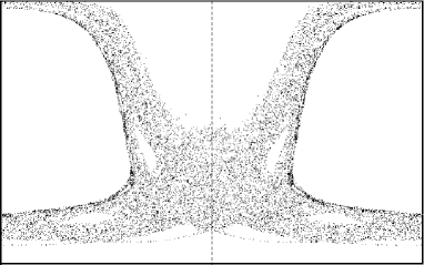
Figure 1: The plot shows a single orbit of the Poincaré map of Eq. (54) at $\theta=0$. The angle $\phi\in[-\pi,\pi]$ is plotted in the horizontal axis and $I_{\phi}\in[0,1]$ in the vertical one. We have taken $\epsilon=0.8$. The energy determines $I_{\theta}$ and its actual value does not affect the dynamics of $\phi$ and $I_{\phi}$.

By examining the plot of Fig. 1, one sees that the orbit densely fills a large region of the Poincaré section and therefore any constant of motion should be the constant function in that region. In the presence of such an ergodic evolution the only constants of motion are functions of the Hamiltonian.

As a consequence we can claim that, genericaly within the Ehrenfest dynamics, the only functions which commute with the Hamiltonian in (53) are those which are function of the Hamiltonian $f_{H}$ itself. As the Poisson bracket is skew-symmetric, the property follows trivially. Ergodicity helps us to assert, roughly speaking, that in general no other function in $\mathcal{O}$ will be a constant of the motion.

Thus, at this stage, we can finish our construction with the equilibrium distribution associated to Ehrenfest dynamics. Taking into account the ergodicity of the dynamics, we can impose the equal-probabilities condition to the configurations of our isolated system, which leads to the microcanonical ensemble, (see Ref. Oliveira and Werlang, 2007). Then, the probability density for the canonical ensemble turns out to be:

$$F_{QC}^{c}(\vec{R},\vec{P},\vec{q},\vec{p})=Z^{-1}e^{-\beta f_{H}},$$ (55)

where $Z=\int_{M_{C}\times S_{Q}}e^{-\beta f_{H}}d\mu_{QC}$, as it can be seen, in a standard derivation, for example in Refs. Balescu, 1997, 1975; Schwabl, 2002, where $\beta^{-1}$, being proportional to the temperature of the isolated system, is the parameter governing the equilibrium between the different parts of the system. An information-theoretic approach to the equiprobability in the microcanonical ensemble and to Eq. (55) may be seen in Ref. Jaynes, 1957 or in Refs. Ellis, 1985; Touchette, 2009 for a much more modern and mathematically sound exposition.

VII Conclusions and future work

In this paper we have constructed a rigorous Hamiltonian description of the Ehrenfest dynamics of an isolated system by combining the Poisson brackets formulation of classical mechanics with the geometric formulation of quantum mechanics. We have also constructed the corresponding statistical description and obtained the associated Liouville equation. Finally, after verifying numerically that the Ehrenfest dynamics is ergodic, we justify the equilibrium distribution produced by it.

The definition of the Hamiltonian in Eq. (40) and its associated canonical equilibrium distribution (55) allows us now to use (classical) Monte Carlo methods for computing canonical equilibrium averages in our system, given by the expression (49).

Also it is straightforward to extend the non-stochastic method proposed by Nosé Nosé (1984, 1991) to our Hamiltonian (40).

However, if we wish to perform MD simulations using stochastic methods, we should first construct the Langevin dynamics associated with our Hamiltonian (40) and equations (41)-(46). To develop this program, we also need an analogue of the Fokker-Planck equation associated with those Langevin equations and then we have to check whether its solution at infinite time approaches (55). Presently we are working on this point Alonso et al. , i.e., on the extension of our formalism to an associated stochastic MD that can be used to rigorously probe non-equilibrium phenomena at constant temperature.