Leptogenesis with TeV Scale Inverse Seesaw in $SO(10)$

Abstract

We discuss leptogenesis within a TeV-scale inverse seesaw model for neutrino masses where the seesaw structure is guaranteed by an $SO(10)$ symmetry. Contrary to the TeV-scale type-I gauged seesaw, the constraints imposed by successful leptogenesis in these models are rather weak and allow for the extra gauge bosons $W_{R}$ and $Z^{\prime}$ to be in the LHC accessible range. The key differences in the inverse seesaw compared to the type I case are: (i) decay and inverse decay rates larger than the scatterings involving extra gauge bosons due to the large Yukawa couplings and (ii) the suppression of the washout due to very small lepton number breaking.

I Introduction

One of the attractive features of the seesaw mechanism for neutrino masses seesaw is that it provides a way to understand the origin of matter in the Universe via leptogenesis fy (for a recent review, see Ref. review ). In the vanilla framework of leptogenesis where right-handed (RH) neutrino masses are hierarchical, it is well known that the lightest RH neutrino needs to be rather heavy, around $10^{9}$ GeV or higher Davidson:2002qv . These scales are however beyond the reach of collider experiments, e.g. the CERN Large Hadron Collider (LHC). On the other hand, from the point of view of the seesaw model itself, one can envisage the new physics scale to be anywhere between TeV to $10^{14}$ GeV. It is well known that the scale of leptogenesis can be lowered to the TeV scale if one allows the RH neutrinos to be quasi-degenerate Pilaftsis . However, first the quasi-degeneracy should be motivated, and second if the scale of the RH neutrinos is to be explained by the breaking of some gauge symmetry, what is the impact of the latter on leptogenesis?

Two classes of seesaw models are of interest in this connection: the usual type-I seesaw seesaw , and the inverse seesaw mv . In both classes of models, a higher gauge symmetry, e.g. $B-L$, is usually called for to make the model “natural”. In addition to providing a compelling reason for the inclusion of the RH neutrinos to guarantee anomaly cancellation, in the type-I case it can be used to understand why the seesaw scale is so much lower than the Planck scale, whereas, in the inverse seesaw case, it stabilizes the zeros in the $(\nu,N,S)$ mass matrix that leads to the doubly-suppressed seesaw formula.

An attractive gauge symmetry that embeds the $B-L$ symmetry and also provides a way to understand the origin of parity violation in low-energy weak interactions is the Left-Right (LR) gauge group $SU(2)_{L}\times SU(2)_{R}\times U(1)_{B-L}$ LR . An important question that arises in these models is: What is the scale of parity invariance? In particular, if it is in the TeV range and if at the same time leptogenesis generates the desired matter-anti-matter asymmetry, then the LHC could be probing neutrino mass physics as well as shed light on one of the deepest mysteries of cosmology.

Since Sakharov’s out-of-equilibrium condition sakharov must be satisfied in order to generate a baryon asymmetry, the existence of new interactions inherent to the LR models make it a nontrivial task to check whether a TeV-scale $W_{R}$ is indeed compatible with leptogenesis as an explanation of the origin of matter. Specifically, the efficiency of leptogenesis crucially depends on the number of RH neutrinos that decay out of equilibrium to produce a leptonic asymmetry. This number is set by two things: First, it depends on the relative magnitudes of the decay rate and the ($C\!P$-conserving) gauge scattering rates of the RH neutrino, since this can lead to a dilution of the number of “useful” RH neutrinos. Second, the washout processes, primarily inverse decays, should drop out of equilibrium early enough, otherwise the number of RH neutrinos gets suppressed at an exponential rate.

These issues have been analyzed for the type-I case within LR symmetric models Frere:2008ct as well as $B-L$ models blanchet . It was found that for the full LR models with TeV-scale parity restoration and RH neutrino masses, gauge scattering rates induced by $W_{R}$ exchange largely dominate the decay and inverse decay rates because the Yukawa couplings are small for the standard type-I seesaw at the TeV scale. These facts lead to a huge dilution of the number of RH neutrinos which decay out of equilibrium and in a $C\!P$ asymmetric manner. Moreover, the gauge scattering interactions also wash out lepton number at a very large rate, much larger than the inverse decays. Altogether, these two effects lead to a very stringent constraint on the mass scale of $W_{R}$ for successful leptogenesis, $M_{W_{R}}\geq 18$ TeV Frere:2008ct , which would imply that the discovery of a $W_{R}$ at the LHC is incompatible with thermal leptogenesis as the origin of matter. On the other hand, in the case of a simple $B-L$ theory, successful leptogenesis only implies that $M_{Z^{\prime}}\geq 2.5$ TeV in the “collider-friendly” region of parameter space where the RH neutrino mass is less than half the $Z^{\prime}$ mass blanchet . We note that there exist bounds on the $W_{R}$ mass from low energy observations bounds and they allow $W_{R}$ mass to be as low as 2.5 TeV.

In this paper, we have analyzed the leptogenesis constraints on the recently proposed TeV-scale LR model within a unified supersymmetric $SO(10)$ framework dev where neutrino masses arise from an inverse seesaw mechanism. Two features distinguish the inverse seesaw mechanism from the type-I seesaw: (i) the Dirac Yukawa couplings of the RH neutrino $N$ can be much larger ($\sim 10^{-1}-10^{-2}$) than for the type-I case (where they are typically of order $\sim 10^{-6}$ for TeV-scale RH neutrino masses) and (ii) the lepton-number-violating parameter (the Majorana mass $\mu$ of the left-right singlet lepton $S$, which measures the “pseudo-Diracness” of $N$) is much smaller than the Dirac mass of $N$. As a result, first, the decay rate of $N$ can be much larger than the $W_{R}$ exchange scattering rate at the baryogenesis epoch, and second, the wash-out processes are suppressed by the small Majorana mass $\mu$. Consequently, we find that both the $W_{R}$ and $Z^{\prime}$ can be in the TeV range and hence accessible at the LHC. This is the main result of our paper, and it should make the case for searching the $W_{R}$ and $Z^{\prime}$ at LHC stronger LHCWR .

This paper is organized as follows: in Section II, we summarize the LR inverse seesaw model and give the Dirac Yukawa couplings as well as the various lepton-number-violating parameters as constrained by $SO(10)$ unification dev . In Section III, we present a generic discussion of leptogenesis in this class of inverse seesaw models; in Section IV, we present the numerical results for our model. Finally, we summarize our findings and conclude in Section V. In Appendix A, we present a new scenario for gauge coupling unification (different from that discussed in Ref. dev ) in these models where the relative magnitudes of $W_{R}$ and $Z^{\prime}$ masses can be unrelated. In Appendix B, we give the analytical expressions of the $C\!P$-asymmetry in the inverse seesaw model for some special cases.

II Left-Right Inverse Seesaw Parameters in $SO(10)$

The implementation of the inverse seesaw mechanism mv requires, in addition to the usual Standard Model (SM) singlet RH neutrinos $N_{i}$ ($i=1,2,3$ for three generations) as in the typical type-I seesaw, three extra SM gauge singlet fermions $S_{i}$ coupled to the RH neutrinos through the lepton-number-conserving couplings of the type ${N}S$, while the traditional RH neutrino Majorana mass term is forbidden by the lepton number symmetry. In the low energy theory, dominant lepton number breaking arises only from the self-coupling term $SS$. The neutrino mass Lagrangian in the flavor basis is given by

$${\cal L}_{\rm mass}={\nu}^{T}C^{-1}M_{D}N+{N}^{T}C^{-1}M_{N}S+\frac{1}{2}S^{T}C^{-1}\mu S+~{}{\rm h.c.},$$ (1)

where $\mu$ is a complex symmetric $3\times 3$ mass matrix containing all the lepton-number-violating parameters, and $M_{D}$ and $M_{N}$ are $3\times 3$ mass matrices representing the Dirac mass terms in the $\nu$–$N$ and $N$–$S$ sectors, respectively. In the basis $\{\nu,N,S\}$, the full $9\times 9$ neutrino mass matrix is then given by

$${\cal M}_{\nu}=\left(\begin{array}[]{ccc}0&M_{D}&0\\ M_{D}^{T}&0&M_{N}\\ 0&M_{N}^{T}&\mu\end{array}\right)\,.$$ (5)

The lepton-number-violating entries in the $\mu$ matrix have to be much smaller than the Dirac neutrino masses in order to fit the light neutrino masses, as observed in neutrino oscillation experiments. In fact, the light neutrino mass matrix can be cast in a seesaw-like form in the limit $\mu\ll M_{D}\ll M_{N}$:

$$m_{\nu}\simeq M_{D}M_{N}^{-1}\mu\left(M_{N}^{T}\right)^{-1}M_{D}^{T}\equiv F\mu F^{T},$$ (6)

to leading order in $F=M_{D}M_{N}^{-1}$. As expected, in the limit $\mu\to 0$, which corresponds to unbroken lepton number, we recover the massless neutrinos of the SM. We note that this smallness of the $\mu$-parameter peculiar to the inverse seesaw models allows for a neutrino mass fit even with TeV-scale RH neutrino mass and large Dirac mass terms. Theoretically, smallness of the $\mu$-term could be explained in extra dimensional brane world models if the lepton number is broken in a separate brane from the standard model brane arkani-hamed .

As shown in Ref. dev , in order to embed a TeV-scale inverse seesaw mechanism into a generic $SO(10)$ model, we need to break the $B-L$ gauge symmetry by 16-Higgs fields at the TeV scale, whereas the $SO(10)$ symmetry is broken down to the LR symmetric gauge group $SU(3)_{c}\times SU(2)_{L}\times SU(2)_{R}\times U(1)_{B-L}$ at the GUT-scale by 45 and 54-Higgs fields; finally, the SM symmetry is broken at the weak scale by 10-Higgs fields. As in the usual $SO(10)$ models, the three generations of quark and lepton fields are assigned to three 16-dimensional spinor representations, and correspondingly, we add three $SO(10)$ singlet matter fields ${\bf 1}_{i}$ (they can be identified with the $S_{i}$ fields above) to implement the inverse seesaw mechanism.

As discussed in Ref. dev , we need at least two ${\bf 10}_{H}$ fields to have a realistic fermion mass spectrum; we also need two ${\bf 45}_{H}$ fields, one for symmetry breaking at the GUT scale and another to give rise to the vectorlike color triplets at the TeV-scale as required by coupling unification constraints. Similarly, we need only the $SU(2)_{R}$ doublet fields of ${\bf 16}_{H}$ and no $SU(2)_{L}$ fields for unification. With this minimal set of Higgs fields, the most general Yukawa superpotential is given by

$$W_{Y} = h_{aij}{\bf 16}_{i}{\bf 16}_{j}{\bf 10}_{H_{a}}+\frac{f_{aij}}{M^{2}}{\bf 16}_{i}{\bf 16}_{j}{\bf 10}_{H_{a}}{\bf 45}_{H}{\bf 45}^{\prime}_{H}+\frac{f^{\prime}_{aij}}{M}{\bf 16}_{i}{\bf 16}_{j}{\bf 10}_{H_{a}}{\bf 45}_{H}$$ (7)

$$+f^{\prime\prime}_{ijk}{\bf 16}_{i}{\bf 1}_{j}\overline{\bf 16}_{H_{k}}+\mu_{ij}{\bf 1}_{i}{\bf 1}_{j},$$

where the first term is the usual Yukawa coupling term, the second and third terms are higher-dimensional terms, and the last two terms give rise to the inverse seesaw mechanism. As already pointed out in Ref. dev , it is sufficient to keep only one of the higher-dimensional operators, usually the ${\bf 16}\cdot{\bf 16}\cdot{\bf 10}\cdot{\bf 45}\cdot{\bf 45^{\prime}}$ term, whose fully antisymmetric combination acts as an effective ${\bf 126}_{H}$ operator, in order to obtain a realistic fermion mass spectrum at the GUT scale, and hence for simplicity, we will assume all the $f^{\prime}$-couplings to be zero; keeping this term does not affect our discussion below .

The $B-L$ symmetry is broken when the ${\overline{\bf 16}}_{H}$-field acquires a vacuum expectation value (VEV) and the $N$–$S$ sector RH neutrino mass matrix is given by

$$M_{N_{ij}}=v_{R}f^{\prime\prime}_{ij},$$ (8)

where $v_{R}$ is the VEV of ${\overline{\bf 16}}_{H}$ and is of order TeV for the low-scale $B-L$ breaking models considered here. All the other fermion masses are generated when the SM symmetry is broken at the weak scale by the ${\bf 10}_{H}$ VEVs. We consider here only the model (A) of Ref. dev where the VEV patterns of the two ${\bf 10}_{H}$ fields are given by

$$\langle\Phi_{1}\rangle=\left(\begin{array}[]{cc}v_{d}&0\\ 0&0\end{array}\right),~{}~{}~{}~{}\langle\Phi_{2}\rangle=\left(\begin{array}[]{cc}0&0\\ 0&v_{u}\end{array}\right),$$ (13)

and the fermion mass matrices are given by

$$M_{u}=\tilde{h}_{u}+\tilde{f},~{}~{}~{}~{}M_{d}=\tilde{h}_{d}+\tilde{f},$$

$$M_{e}=\tilde{h}_{d}-3\tilde{f},~{}~{}~{}~{}M_{D}=\tilde{h}_{u}-3\tilde{f},$$ (14)

where in the notation of Ref. dev , $\tilde{h}_{u,d}\equiv v_{u,d}h_{u,d}$ and $\tilde{f}\equiv v_{u}f_{u}=v_{d}f_{d}$. Using the renormalization group evolution of the fermion masses in the LR model, we obtain the GUT-scale fermion masses starting from the experimentally known weak scale values, and using these mass eigenvalues, we obtain a fit for the Yukawa coupling matrices at the GUT scale, from which we can get the structure of the Dirac neutrino mass matrix.  Here, as an example, we quote the result for $\tan\beta\equiv v_{u}/v_{d}=10$ dev :

$$M_{D}=\left(\begin{array}[]{ccc}0.0111&0.0384-0.0103{\rm i}&0.038-0.4433{\rm i}\\ 0.0384+0.0103{\rm i}&0.2928&1.8623+0.0002{\rm i}\\ 0.038+0.4433{\rm i}&1.8623-0.0002{\rm i}&77.7573\end{array}\right)~{}{\rm GeV}.$$ (18)

With this Dirac neutrino mass, we can easily fit the observed neutrino oscillation data by fixing the singlet mass matrix $\mu$ in Eq. (6). As an example, for a normal hierarchy of neutrino masses, and assuming a diagonal structure for the RH neutrino mass matrix $M_{N}$ with eigenvalues (3.5, 3, 1) TeV, we can fit the observed $2\sigma$ neutrino oscillation data fogli for the following choice of $\mu$:

$$\mu=\left(\begin{array}[]{ccc}-17.4226+0.3098{\rm i}&2.1033-0.0590{\rm i}&-0.0136+0.0288{\rm i}\\ 2.1033-0.0590{\rm i}&-0.2585+0.0097{\rm i}&0.0016-0.0035{\rm i}\\ -0.0136+0.0288{\rm i}&0.0016-0.0035{\rm i}&3.6\times 10^{-5}+4.6\times 10^{-5}{\rm i}\end{array}\right)~{}{\rm GeV}.$$ (22)

III Leptogenesis in Left-Right Inverse Seesaw Models

In this section we summarize the main features of leptogenesis within the class of LR inverse seesaw models discussed above. We also wish to note that while we have used the $SO(10)$ framework to make the results definite and somewhat more predictive, our discussion applies also to the case with TeV-scale Left-Right symmetry without grand unification. In what follows, we will partially follow the discussion presented in Ref. Blanchet:2009kk .

As discussed in the introduction, a crucial difference of the inverse seesaw from the usual seesaw is the dependence on a new mass matrix, $\mu$, which can lead to the result that no matter what the ratio of the mass scales $M_{D}/M_{N}$ is, the lightness of the left-handed neutrinos can always be explained by small $\mu$ entries. In other words, the inverse seesaw makes it possible to have at the same time large Dirac masses and low, say TeV-scale, RH neutrino masses, and it still can explain why neutrinos are light. This is directly connected to the fact that, in the limit $\mu\to 0$, lepton number is conserved, and therefore neutrino masses vanish, as in the SM. This is a crucial difference from the case of TeV scale type I seesaw.

An interesting question to ask is how leptogenesis is affected by this distinctive feature of inverse seesaw models. We expect that the lepton-number-violating washout will go to zero in the limit of vanishing $\mu$. As a matter of fact, as explicitly shown in Ref. Blanchet:2009kk , the all-important $\Delta L=2$ washout process $\ell\Phi\to\bar{\ell}\Phi^{\dagger}$ vanishes as $\delta_{i}^{2}$, with

$$\delta_{i}=\frac{|M_{i}-M_{j}|}{\Gamma_{i}}\simeq\frac{\mu_{ii}}{\Gamma_{i}}\,,$$ (23)

where $\Gamma_{i}$ is the total decay rate of $N_{i}$ into lepton and Higgs (and antiparticles), and $M_{i,j}$ are the masses of the quasi-Dirac RH neutrino pair $N_{i,j}$ (with $\Gamma_{i}\simeq\Gamma_{j}$). Note that we denote by $M_{i}~{}(i=1,\ldots,6)$ the heavy neutrino mass eigenvalues. As shown in the Appendix, the leading order contribution to the mass splitting for each quasi-Dirac pair comes from the diagonal elements of the $\mu$ matrix. Therefore, as expected, the washout tends to zero in the limit of vanishing $\mu$. The suppression of the washout can be shown to occur through the destructive interference of one member of a quasi-Dirac pair with the other Blanchet:2009kk . It is instructive to show numerically how the washout is kept under control in this family of models with more than one pair of RH neutrinos. The washout parameter $K_{i}$ is defined as

$$K_{i}={\Gamma_{i}\over H(z=1)}={(hh^{\dagger})_{ii}v_{u}^{2}\over m_{\star}M_{i}}\,,$$ (24)

where $H(z)$ is the usual Hubble expansion rate: $H(z)\simeq 1.66\sqrt{g_{*}}\frac{M_{i}^{2}}{z^{2}M_{\rm Pl}}$, and $m_{\star}\simeq 1.08\times 10^{-3}$ eV. Plugging in numbers, we find that with Yukawa couplings of order $10^{-1}$ and a RH neutrino mass of order 1 TeV, the washout parameter $K$ is of order $10^{12}$, which is huge! However, the suppression of the washout is also very large, being proportional to $\delta^{2}$ with $\delta\ll 1$ due to the smallness of $\mu$, as required to get the right scale for the light neutrinos. Specifically, for the example of Eq. (22), we find that $\delta\sim 10^{-5}$ and therefore the effective washout parameter $K^{\rm eff}\simeq\delta^{2}K\sim 100$, which is reasonably small.

In the LR model we are considering, there are other processes contributing to the washout of lepton number, for instance, $N_{R}e_{R}\leftrightarrow\bar{u}_{R}d_{R}$. More precisely, this process destroys RH lepton number, but in the temperature range of interest to us (TeV scale) every individual RH lepton flavor equilibrates with the LH lepton flavor one, thanks to the Yukawa interactions. Does this process also turn off in the limit of lepton number conservation? It can be easily shown that, including the production of the RH neutrino by an inverse decay, followed by the scattering process mentioned above, there is also a destructive interference within the quasi-Dirac pair which leads exactly to the same kind of $\delta^{2}$-suppression as for the process $\ell\Phi\to\bar{\ell}\Phi^{\dagger}$.

Another feature of inverse seesaw models is that they typically lead to lepton flavor equilibration AristizabalSierra:2009mq because of the large Yukawa couplings. More precisely, it can be shown that the process $\ell_{\alpha}\Phi\leftrightarrow\ell_{\beta}\Phi$, which does not change lepton number, but changes lepton flavor, is deep in thermal equilibrium for the TeV temperatures (see, for instance, Ref. Antusch:2009gn ). Consequently, the Boltzmann equations for leptogenesis can be written as only one equation for the sum of the lepton flavors AristizabalSierra:2009mq . In other words, flavor effects flavor are not important in our framework.

Putting together all the qualitatively important effects discussed above and solving the relevant set of Boltzmann equations, one can derive the following expression for the efficiency factor (see, for instance, Ref. pedestrian ):

$$\kappa_{i}(z) \simeq \int_{z_{0}}^{z}dz^{\prime}\frac{dN^{\rm eq}_{N_{i}}(z^{\prime})}{dz^{\prime}}\frac{D(K_{i},z^{\prime})}{D(K_{i},z^{\prime})+D_{W_{R}}(z^{\prime})+4S_{Z^{\prime}}N_{N_{i}}^{\rm eq}({z^{\prime}})+S_{W_{R}}(z^{\prime})}$$ (25)

$$\times{\rm exp}\left[-\int_{z^{\prime}}^{z}dz^{\prime\prime}\left\{\sum_{i}W_{\rm ID}(K_{i},z^{\prime\prime})+W_{W_{R}}(z^{\prime\prime})\right\}\delta_{i}^{2}\right]\,,$$

where $z\equiv M_{i}/T$,  $N_{X}$ is the number density of $X$ over the relativistic number density of RH neutrinos, and $D,~{}S,~{}W$ denote the various decay, scattering and washout terms respectively, defined in Section IV. Note that the expression above assumes $dN_{N_{i}}/dz\simeq dN^{\rm eq}_{N_{i}}/dz$ with $N_{N_{i}}^{\rm eq}=\frac{1}{2}z^{2}{\cal K}_{2}(z)$,  where ${\cal K}_{2}(z)$ is the modified Bessel function of the 2nd kind. This is a very good approximation in our model (with large Yukawa couplings). Note also that we are neglecting spectator processes spec and $\Delta L=1$ scatterings involving the Higgs, which are both expected to lead to order one corrections.

The final baryon asymmetry can be conveniently written as

$$\eta_{B}\simeq 10^{-2}\sum_{i}\epsilon_{i}\kappa_{i}(z\to\infty)\,,$$ (26)

where the dilution factor $10^{-2}$ takes into account the fraction of $B-L$ asymmetry converted into baryon asymmetry by sphaleron processes and also the dilution due to photon production from the onset of leptogenesis till recombination. $\epsilon_{i}$ is the $C\!P$-asymmetry generated by the decay of $N_{i}$ into any lepton flavor and is given by Covi:1996wh

$$\epsilon_{i}=\frac{1}{8\pi}\sum_{j\neq i}{{\rm Im}\left[(hh^{\dagger})^{2}_{ij}\right]\over\sum_{\beta}|h_{i\beta}|^{2}}f^{v}_{ij}$$ (27)

where $f^{v}$ is the $L$-violating self-energy and vertex loop factor. In the quasi-degenerate limit of the $(i,j)$ pair, we have

$$f^{v}_{ij}\simeq\frac{M_{j}^{2}-M_{i}^{2}}{(M_{j}^{2}-M_{i}^{2})^{2}+(M_{j}\Gamma_{j}-M_{i}\Gamma_{i})^{2}}\,.$$ (28)

Note that Eq. (27) was derived assuming heavy neutrino mass eigenstates. Therefore, it is necessary to make a basis transformation from the “flavor” basis where

$${\cal M}_{\rm RH}=\left(\begin{array}[]{cc}0&M_{N}\\ M_{N}^{T}&\mu\end{array}\right),$$ (31)

to the diagonal mass basis with real and positive eigenvalues $M_{i}~{}(i=1,2,\ldots,6)$, grouped into three quasi-degenerate pairs with mass splittings in each pair of order $\mu_{kk}~{}(k=1,2,3)$. Analytically, the exact diagonalization of the full $6\times 6$ mass matrix ${\cal M}_{\rm RH}$ to get a closed form expression for the Yukawa couplings, $h_{i\alpha}$, in terms of the known parameters, namely $M_{D},~{}M_{N}$ and $\mu$, is extremely involved. In Appendix B, we show the analytical expressions up to first order in $\mu$ for some simpler cases with only two quasi-Dirac pairs and show explicitly that the $C\!P$-asymmetry indeed vanishes in the $L$-conserving limit $\mu\to 0$, as expected. For the general case with three quasi-Dirac pairs, we numerically evaluate the $C\!P$-asymmetry in the next section. We note that the three-pair case reduces to the two-pair case discussed in Appendix B if one of the masses is much heavier than the other two and hence decouples from the rest.

IV Results

As noted in Section II, the Yukawa couplings are fixed by the $SO(10)$ symmetry. The $\mu$ matrix can be deduced from the knowledge of the light neutrino masses and mixing angles as a function of the RH neutrino mass matrix $M_{N}$, which can be taken to be diagonal without loss of generality. Varying the RH neutrino mass eigenvalues input then leads to different $\mu$ matrices, keeping the light neutrino mass matrix given by Eq. (6) such that its mass eigenvalues and mixing angles are within $2\sigma$ of the observed values. Once we know the explicit form of the RH neutrino mass matrix given by Eq. (31), we can define the quasi-Dirac pairs by transforming to a basis in which this mass matrix is diagonal with real and positive eigenvalues. We then calculate the $C\!P$-asymmetry and efficiency factors for the decay of the lightest RH neutrino pair and scan the parameter space to match the calculated baryon asymmetry (using Eq. (26)) with the observed 68% C.L. value, $\eta_{B}=(6.2\pm 0.15)\times 10^{-10}$ wmap . Note that we only consider the asymmetry generated by decay of the lightest RH neutrino pair as the asymmetry generated by the heavy pairs is washed out very rapidly (due to large exponential suppression), and for these washouts not to affect the asymmetry generated by the lightest pair, we require the lightest pair to be at least 3 times smaller than the next heavy pair Blanchet:2006dq .

To calculate the efficiency factor given by Eq. (25), we first write down the thermally averaged rates for $N\to\ell\Phi$ decay and the corresponding inverse decay pedestrian :

$$D(K_{i},z) = \frac{{\cal K}_{1}(z)}{{\cal K}_{2}(z)}K_{i}z,$$

$$W_{\rm ID}(K_{i},z) = \frac{1}{4}K_{i}{\cal K}_{1}(z)z^{3}.$$ (32)

with ${\cal K}_{a},~{}a=1,2$ denoting the modified Bessel function of the $i$th type. The thermally averaged rate $D_{W_{R}}$ for the $W_{R}$-mediated $N$-decay, $N\to\ell q_{R}\bar{q}^{\prime}_{R}$, is given by

$$D_{W_{R}}(z)=\frac{\gamma_{N}^{(W_{R})}}{n^{\rm eq}_{N}Hz}$$ (33)

where $n_{N}^{eq}$ is the RH neutrino equilibrium number density, $n_{N}^{\rm eq}(z)=\frac{3}{4}n_{\gamma}(z)N_{N_{i}}^{\rm eq}(z)$ with $n_{\gamma}=\frac{2\zeta(3)}{\pi^{2}}T^{3}$, and $\gamma_{N}$ is the reaction density:

$$\gamma_{N}^{(W_{R})}=n_{N}^{\rm eq}(z)\frac{{\cal K}_{1}(z)}{{\cal K}_{2}(z)}\Gamma_{N}^{(W_{R})},$$ (34)

where $\Gamma_{N}^{(W_{R})}$ is the total three body decay width of $N$, given by Frere:2008ct

$$\Gamma_{N}^{W_{R}}=\frac{3g_{R}^{4}}{2^{9}\pi^{3}M_{N}^{3}}\int_{0}^{M_{N}^{2}}ds\frac{(M_{N}^{6}-3M_{N}^{2}s^{2}+2s^{3})}{(s-M_{W_{R}}^{2})^{2}+M_{W_{R}}^{2}\Gamma_{W_{R}}^{2}}\,.$$ (35)

with the $W_{R}$ total decay width $\Gamma_{W_{R}}=\frac{g_{R}^{2}}{4\pi}M_{W_{R}}$.

The various scattering rates $S_{W_{R},Z^{\prime}}$ appearing in Eq. (25) are also defined as in Eq. (33) where the corresponding scattering reaction density is related to the reduced cross section as follows (see, for instance, Ref. Giudice:2003jh ):

$$\gamma(ab\leftrightarrow cd)=\frac{M_{N}^{4}}{64\pi^{4}z}\int_{x_{\rm thr}}^{\infty}dx\sqrt{x}\hat{\sigma}(x){\cal K}_{1}(z\sqrt{x})$$ (36)

with $x=s/M_{N}^{2}$ and the threshold value $x_{\rm thr}=\frac{1}{M_{N}^{2}}{\rm max}[(m_{a}+m_{b})^{2},(m_{c}+m_{d})^{2}]$. The reduced cross sections for various $W_{R}$ exchange diagrams were computed in Ref. Frere:2008ct :

$$\hat{\sigma}_{Ne_{R}\leftrightarrow\bar{u}_{R}d_{R}}(x) = \frac{9g_{R}^{4}}{48\pi x}\frac{(1-3x^{2}+2x^{3})}{\left[\left(x-\frac{M_{W_{R}}^{2}}{M_{N}^{2}}\right)^{2}+\frac{M_{W_{R}}^{2}\Gamma_{W_{R}}^{2}}{M_{N}^{4}}\right]}\,,$$ (37)

$$\hat{\sigma}_{N\bar{u}_{R}\leftrightarrow e_{R}\bar{d}_{R}}(x) = \frac{9g_{R}^{4}}{8\pi x}\int_{1-x}^{0}du\frac{(x+u)(x+u-1)}{\left(u-\frac{M_{W_{R}}^{2}}{M_{N}^{2}}\right)^{2}}\,,$$ (38)

$$\hat{\sigma}_{Nd_{R}\leftrightarrow e_{R}u_{R}}(x) = \frac{9g_{R}^{4}}{8\pi}\frac{M_{N}^{2}}{M_{W_{R}}^{2}}\frac{(1-x)^{2}}{\left(x+\frac{M_{W_{R}}^{2}}{M_{N}^{2}}-1\right)}\,,$$ (39)

Here we have ignored the $t$-channel process $NN\to\ell\ell$ as the rate for this process falls off very rapidly for the region of interest, viz. $z>1$ Frere:2008ct .

The reduced cross section for the $Z^{\prime}$ exchange diagram is given by Plumacher:1996kc

$$\hat{\sigma}_{NN\leftrightarrow\ell\bar{\ell},q\bar{q}}(x)=\frac{13g_{B-L}^{4}}{6\pi}\frac{\sqrt{x(x-4)^{3}}}{\left(x-\frac{M_{Z^{\prime}}^{2}}{M_{N}^{2}}\right)^{2}+\frac{M_{Z^{\prime}}^{2}\Gamma_{Z^{\prime}}^{2}}{M_{N}^{4}}}\,,$$ (40)

with the total $Z^{\prime}$ decay width

$$\Gamma_{Z^{\prime}}=\frac{g_{B-L}^{2}}{24\pi}M_{Z^{\prime}}\left[13+3\left(1-\frac{4M_{N}^{2}}{M_{Z^{\prime}}^{2}}\right)^{3/2}\right]\,.$$ (41)

Before calculating the efficiency factor, it is instructive to compare all the reaction rates appearing in Eq. (25) to get a clear idea of various contributions. As an illustration, we consider the case with the RH Majorana neutrino mass eigenvalues $(3.5,3,1)$ TeV (as in Eq. (22)). The flavor-summed washout parameter for the decay of the lightest quasi-Dirac pair in this case is given by $K_{3}\simeq 4\times 10^{11}$ whereas the effective washout parameter is given by $K_{3}^{\rm eff}\simeq\delta_{3}^{2}K_{3}\simeq 168$ which is reasonable. For comparison, the corresponding values for the two heavy pairs are $K_{1}^{\rm eff}\simeq K_{2}^{\rm eff}=8\times 10^{7}$ which, when exponentiated in the washout term in Eq. (25), leads to a huge suppression, thus making the efficiency in those channels practically negligible. Hence, from now on, we will consider the decay of only the lightest pair.

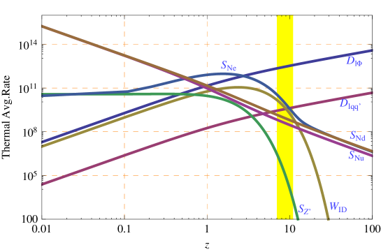
Figure 1: Various $N$ decay and scattering rates (thermally averaged) as a function of $z=M_{N_{3}}/T$ for a particular choice of RH neutrino masses, $(M_{N_{1}},M_{N_{2}},M_{N_{3}})=(3.5,3,1)$ TeV and $M_{W_{R}}=M_{Z^{\prime}}=2$ TeV. The yellow shaded region is where the asymmetry is generated.

In Fig. 1, we show the various thermally averaged decay and scattering rates as a function of $z\equiv M_{N_{3}}/T$, for the above choice of the RH neutrino masses and for $M_{W_{R}}=M_{Z^{\prime}}=2$ TeV. The yellow shaded region shows the asymmetry production time, approximately when $z_{B}-2<z<z_{B}+2$ with $z_{B}\simeq 2+4K^{0.13}e^{-2.5/K}\simeq 9$ Antusch:2009gn . We note that in this range, the $N\to\ell\Phi$ decay rate, $D_{\ell\Phi}$, dominates over the three-body decay rate as well as all the scattering rates by several orders of magnitude. Hence in the efficiency factor, Eq. (25), the dilution term $D/(D+S)$ is very close to unity and is essentially independent of $M_{W_{R}}$ and $M_{Z^{\prime}}$. The enhanced $N\to\ell\Phi$ decay rate is due to the large Yukawa couplings in the inverse seesaw scenario. We also note that as the $W_{R}$-mediated three-body $N$ decay rate is much smaller than the $N\to\ell\Phi$ decay rate, the washout term $W_{W_{R}}$ in Eq. (25) arising due to the process $\ell\Phi\to N\to\bar{\ell}q\bar{q}^{\prime}$ which is proportional to the branching ratio of $N\to\bar{\ell}q\bar{q}^{\prime}$ will be suppressed compared to the inverse decay term $W_{\rm ID}$. Thus we find that the efficiency factor is also essentially independent of both $W_{R}$ and $Z^{\prime}$ masses for a wide range of parameter space. Of course, the $W_{R}$ and $Z^{\prime}$ scattering terms will start to dominate for very low values of their masses; however, we estimated this lower bound to be well below the current collider bounds on $M_{W_{R}}$ and $M_{Z^{\prime}}$ which are roughly a TeV or so WRbound .

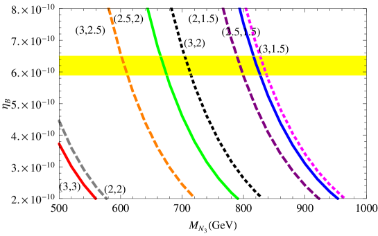
Figure 2: Correlation between the baryon asymmetry and the lightest RH neutrino mass for various heavy mass pairs $(M_{N_{1}},M_{N_{2}})$ in TeV. The yellow shaded region is the observed value of $\eta_{B}$ within $2\sigma$ C.L..

Fig. 2 shows the baryon asymmetry $\eta_{B}$ as a function of the lightest RH neutrino mass $M_{N_{3}}$ for different choices of the heavy RH neutrino masses $(M_{N_{1}},M_{N_{2}})$ from $1.5-3$ TeV. The calculated value of $\eta_{B}$ is to be compared with the observed 68% C.L. value, $\eta_{B}=(6.2\pm 0.15)\times 10^{-10}$ wmap . It is clear from the figure that for a given heavy mass pair, there is a narrow range of values allowed for $M_{N_{3}}$ satisfying the observed baryon asymmetry (the yellow shaded region). We note that for fixed $M_{N_{1}}$, the allowed range of $M_{N_{3}}$ decreases with increasing $M_{N_{2}}$, while for fixed $M_{N_{2}}$, the allowed range of $M_{N_{3}}$ increases with increasing $M_{N_{1}}$. Also note that when the heavy pairs have degenerate mass, the baryon asymmetry gets suppressed (e.g. the lower two lines in Fig. 2) due to the suppression in the $C\!P$-asymmetry. Finally, we note that for a given set of heavy mass pairs, $\eta_{B}\propto M_{N_{3}}^{-3}$.

Fig. 3 shows the correlation between the efficiency factor and the flavor-summed $C\!P$ asymmetry for various channels. The different lines correspond to different values of the heavy mass pair, $(M_{N_{1}},M_{N_{2}})$ in TeV, starting from (3,1.5) TeV at the top to (3,3) TeV at bottom. We note that for fixed $M_{N_{1}}$, the lines move down as we increase $M_{N_{2}}$ while for fixed $M_{N_{2}}$, they move up with increasing $M_{N_{1}}$. The yellow shaded region shows the observed value of $\eta_{B}$ which is essentially the product of $\kappa$ and $\epsilon$, summed over all pairs. As we have pointed out earlier, only the lightest pair contribution is significant, while the efficiency is too small for the other two pairs.

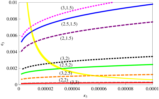
Figure 3: Correlation between the efficiency factor and the flavor-summed $C\!P$-asymmetry for the lightest pair for various values of the heavy mass pair $(M_{N_{1}},M_{N_{2}})$ in TeV. The yellow shaded region corresponds to the observed value of $\eta_{B}$ within $2\sigma$ C.L..

V Conclusion

In summary, we have shown that a TeV-scale Left-Right symmetry can be compatible with the understanding of the origin of matter via leptogenesis provided small neutrino masses are understood using the inverse seesaw mechanism. A crucial feature of this mechanism is that the magnitude of the lepton-number-breaking Majorana mass term is directly proportional to the neutrino mass, rather than inversely as in the usual type-I seesaw framework. This allows the Yukawa couplings that generate the Dirac mass for the neutrinos close to one, even with TeV-scale RH neutrinos. These two facts help to keep the wash-out of the generated lepton asymmetry under control, and thus explain the origin of matter while keeping both the $Z^{\prime}$ and $W_{R}$ in the TeV range. The results of this paper should provide new motivation for searching for the $W_{R}$ and the Left-Right $Z^{\prime}$ at the LHC. As has been already emphasized in literature LHCWR , the signal for the inverse seesaw with $W_{R}$ would be presence of trilepton final states with missing energy.

Appendix A A New Coupling Unification Scenario

It was shown in Ref. dev that the $SO(10)$ embedding of TeV-scale inverse seesaw mechanism discussed in this paper is consistent with gauge coupling unification. In particular, it was shown that for the symmetry breaking chain

$$SO(10)\stackrel{{\scriptstyle M_{G}}}{{\longrightarrow}}{\bf 3}_{c}{\bf 2}_{L}{\bf 2}_{R}{\bf 1}_{B-L}~{}({\rm SUSYLR)}~{}\stackrel{{\scriptstyle M_{R}}}{{\longrightarrow}}{\bf 3}_{c}{\bf 2}_{L}{\bf 1}_{Y}~{}({\rm MSSM})~{}\stackrel{{\scriptstyle M_{S}}}{{\longrightarrow}}{\bf 3}_{c}{\bf 2}_{L}{\bf 1}_{Y}~{}({\rm SM})~{}\stackrel{{\scriptstyle M_{Z}}}{{\longrightarrow}}{\bf 3}_{c}{\bf 1}_{Q},$$

and for TeV-scale SUSY and $B-L$ breaking, it is possible to obtain gauge coupling unification with two ${\bf 10}_{H}$ bidoublets, two RH ${\bf 16}_{H}$ doublets and one ${\bf 45}_{H}$ color triplet. In this section, we show that there is an alternative choice of Higgs fields which also leads to coupling unification with TeV-scale $W_{R}$ and $Z^{\prime}$. If we add one set of $SU(2)_{R}$ triplets, $\Delta(1,1,3,0)$, coming from the ${\bf 45}_{H}$ field, then we can also achieve unification with the same field content as above except that we need only one $SU(2)_{R}$ doublet. The SUSYLR $\beta$-function in this model is given by

$$b_{i}=\left(10+\frac{3}{2}n_{L}+\frac{3}{2}n_{R},n_{10}+n_{L},n_{10}+n_{R}+2,-2\right)=\left(\frac{23}{2},2,3,-2\right)~{}~{}(i={\bf 1}_{B-L},{\bf 2}_{L},{\bf 2}_{R},{\bf 3}_{c})$$

for $n_{10}=2,~{}n_{L}=0$ and $n_{R}=1$. As shown in Fig. 4, we achieve unification at $M_{G}\simeq 4\times 10^{16}$ GeV with $\alpha_{U}^{-1}\simeq 20.3$.

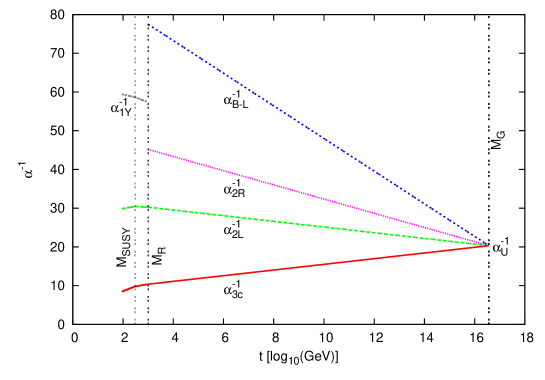
Figure 4: Gauge coupling unification in the new $SO(10)$ scenario with one $SU(2)_{R}$ doublet and one $SU(2)_{R}$ triplet.

This model has two nice features over the previous one: (i) all the Higgs fields required for unification are connected to breaking of separate gauge symmetries and there is no arbitrariness in the number of fields, and (ii) the presence of the $SU(2)_{R}$ triplet enables us to decouple the mass scales $M_{W_{R}}$ and $M_{Z^{\prime}}$ which are otherwise related in usual Left-Right models with $M_{Z^{\prime}}>M_{W_{R}}$.

Appendix B Analytical Expression for the $C\!P$-Asymmetry

The full Majorana mass matrix in the flavor basis $(N_{i},S_{i})$ is given by

$${\cal M}=\left(\begin{array}[]{cc}0&M_{N}\\ M^{T}_{N}&\mu\end{array}\right)$$ (44)

where for $i=1,2,3$, both $M_{N}$ and $\mu$ are $3\times 3$ symmetric matrices. The Yukawa Lagrangian in this basis is given by (with $i,j=1,2,3$)

$${\cal L}_{y}=y_{i\alpha}\overline{N}_{i}\Phi^{\dagger}l_{\alpha}+M_{N_{ij}}N_{i}^{T}C^{-1}S_{j}+\frac{1}{2}\mu_{ij}S_{i}^{T}C^{-1}S_{j}+~{}{\rm h.c.}$$ (45)

In order to calculate the $C\!P$ asymmetry in this framework, it is more convenient to work in the basis in which the RH Majorana neutrino mass matrix is diagonal with real and positive eigenvalues. The Lagrangian in this basis is given by (with $i=1,2,\cdots,6$)

$${\cal L}_{h}=h_{i\alpha}\overline{\tilde{N}}_{i}\Phi l_{\alpha}+\frac{1}{2}M_{i}\tilde{N}_{i}^{T}C^{-1}\tilde{N}_{i}+{\rm h.c.}$$ (46)

Analytically, the exact diagonalization of the full $6\times 6$ mass matrix ${\cal M}$ is extremely involved and we cannot obtain a closed form expression for the $C\!P$-asymmetry in this case. However, we can study the dependence of the small $L$-violating parameter $\mu$ in some special cases, viz. when the $\mu$-matrix is completely diagonal or completely off-diagonal, as in these cases the Majorana mass matrix reduces to a block diagonal form. In this section, we derive the analytical expression for the $C\!P$-asymmetry in these two limits and for two sets of RH neutrinos, i.e. for $(N_{i},S_{i})$ with $i=1,2$. The $i=3$ case reduces to this limit if one of the masses is much heavier and hence decouples from the other two.

We consider the $4\times 4$ version of the Majorana mass matrix ${\cal M}$:

$${\cal M}_{4\times 4}=\left(\begin{array}[]{cc}0&M_{N_{2\times 2}}\\ M_{N_{2\times 2}}&\mu_{2\times 2}\end{array}\right)\,,$$ (49)

where without loss of generality we choose the mass matrix $M_{N}$ to be diagonal with real positive eigenvalues $M_{N_{1,2}}$. However, the elements of the $\mu$-matrix are, in general, complex quantities. Now we consider two special cases:

Case-I: $\mu$ purely diagonal

In this case, the Majorana mass matrix can be reduced to a simple block diagonal form which decouples the $(N_{1},S_{1})$ and $(N_{2},S_{2})$ sectors:

$${\cal M}=\left(\begin{array}[]{cccc}0&0&M_{N_{1}}&0\\ 0&0&0&M_{N_{2}}\\ M_{N_{1}}&0&\mu_{11}&0\\ 0&M_{N_{2}}&0&\mu_{22}\end{array}\right)\stackrel{{\scriptstyle r_{2}\leftrightarrow r_{3},c_{2}\leftrightarrow c_{3}}}{{\longrightarrow}}\left(\begin{array}[]{cccc}0&M_{N_{1}}&0&0\\ M_{N_{1}}&\mu_{11}&0&0\\ 0&0&0&M_{N_{2}}\\ 0&0&M_{N_{2}}&\mu_{22}\end{array}\right)\,.$$ (58)

Then in the $(N_{i},S_{i})$ flavor basis, we have the $2\times 2$ matrices

$$\tilde{M}_{i}=\left(\begin{array}[]{cc}0&M_{N_{i}}\\ M_{N_{i}}&\mu_{ii}\end{array}\right)=\left(\begin{array}[]{cc}0&M_{N_{i}}\\ M_{N_{i}}&\varepsilon_{i}M_{N_{i}}e^{{\rm i}\theta_{i}}\end{array}\right)\,,$$ (63)

where $\varepsilon_{i}\equiv\mu_{ii}/M_{N_{i}}\ll 1$. The $\tilde{M}_{i}$ is diagonalized with real and positive eigenvalues by a unitary transformation $U_{i}^{T}\tilde{M}_{i}U_{i}$ where

$$U_{i}=\left(\begin{array}[]{cc}-{\rm i}\cos{\alpha_{i}}e^{{\rm i}\theta_{i}/2}&\sin{\alpha_{i}}e^{{\rm i}\theta_{i}/2}\\ {\rm i}\sin{\alpha_{i}}e^{-{\rm i}\theta_{i}/2}&\cos{\alpha_{i}}e^{-{\rm i}\theta_{i}/2}\end{array}\right)\,,$$ (66)

and the mixing angles are given by

$$\cos{\alpha_{i}}\simeq\frac{1}{\sqrt{2}}\left(1+\frac{\varepsilon_{i}}{4}\right),~{}~{}\sin{\alpha_{i}}\simeq\frac{1}{\sqrt{2}}\left(1-\frac{\varepsilon_{i}}{4}\right)\,,$$ (67)

up to ${\cal O}(\varepsilon_{i})$. The corresponding mass eigenvalues are given by

$$M_{j}\simeq M_{N_{i}}\left(1\pm\frac{\varepsilon_{i}}{2}\right)~{}~{}(i=1,2;~{}j=1,2,3,4)\,.$$ (68)

It is clear that the mass splitting within a quasi-Dirac pair is given by $\mu_{ii}$.

The Yukawa couplings in this diagonal mass basis are related to the couplings in the flavor basis as follows:

$$h_{1\alpha} \simeq \frac{{\rm i}e^{-{\rm i}\theta_{1}/2}}{\sqrt{2}}\left(1+\frac{\varepsilon_{1}}{4}\right)y_{1\alpha},$$

$$h_{2\alpha} \simeq \frac{e^{-{\rm i}\theta_{1}/2}}{\sqrt{2}}\left(1-\frac{\varepsilon_{1}}{4}\right)y_{1\alpha},$$

$$h_{3\alpha} \simeq \frac{{\rm i}e^{-{\rm i}\theta_{2}/2}}{\sqrt{2}}\left(1+\frac{\varepsilon_{2}}{4}\right)y_{2\alpha},$$

$$h_{4\alpha} \simeq \frac{e^{-{\rm i}\theta_{2}/2}}{\sqrt{2}}\left(1-\frac{\varepsilon_{2}}{4}\right)y_{2\alpha}.$$ (69)

Note that in the $L$-conserving limit $\varepsilon_{i}\to 0$, we have $h_{i\alpha}={\rm i}h_{j\alpha}$ within a quasi-degenerate pair $(i,j)$, as expected.

Now let us calculate the $C\!P$-asymmetry for the decay of one of the quasi-Dirac particles, say $i=1$. We have from Eq. (27),

$$\epsilon_{1}=\frac{1}{8\pi}\sum_{j\neq 1}\frac{{\rm Im}\left[(hh^{\dagger})^{2}_{1j}\right]}{\sum_{\beta}|h_{1\beta}|^{2}}f^{v}_{1j}\simeq\frac{\varepsilon_{2}}{16\pi\sum_{\beta}|y_{1\beta}|^{2}}{\rm Im}\left[e^{{\rm i}(\theta_{1}-\theta_{2})}\left(\sum_{\alpha}y^{*}_{1\alpha}y_{2\alpha}\right)^{2}\right]f^{v}_{13}$$ (70)

assuming $f_{13}\simeq f_{14}$. Note that the $j=2$ term vanishes as there is no imaginary part in that case. It is clear that $\epsilon_{1}$ vanishes as $\mu_{22}\to 0$. Similarly, one can show that $\epsilon_{2}$ also vanishes in the limit $\mu_{22}\to 0$, and $\epsilon_{3},~{}\epsilon_{4}$ vanish as $\mu_{11}\to 0$.

Case II: $\mu$ purely off-diagonal

In this case, the Majorana mass matrix in the $(N_{i},S_{i})$ flavor basis reduces to the following block diagonal form:

$${\cal M}=\left(\begin{array}[]{cccc}0&0&M_{N_{1}}&0\\ 0&0&0&M_{N_{2}}\\ M_{N_{1}}&0&0&\mu_{12}\\ 0&M_{N_{2}}&\mu_{12}&0\end{array}\right)\stackrel{{\scriptstyle c_{1}\leftrightarrow c_{3},r_{2}\leftrightarrow r_{4}}}{{\longrightarrow}}\left(\begin{array}[]{cccc}M_{N_{1}}&0&0&0\\ \mu_{12}&M_{N_{2}}&0&0\\ 0&0&M_{N_{1}}&\mu_{12}\\ 0&0&0&M_{N_{2}}\end{array}\right)\,,$$ (79)

which, however, mixes the (1,2) sectors; in the $(N_{1},S_{2})$ basis, we have the $2\times 2$ mass matrix

$$\tilde{M}=\left(\begin{array}[]{cc}M_{N_{1}}&0\\ \mu e^{{\rm i}\theta}&M_{N_{2}}\end{array}\right)\,,$$ (82)

with $\mu\ll M_{N_{1}},M_{N_{2}}$. However, unlike in Case I, we cannot diagonalize this asymmetric matrix by a single unitary transformation; instead, we have to apply a bi-unitary transformation of the form $V^{\dagger}\tilde{M}U$. We find that the following forms of $U$ and $V$ diagonalize $\tilde{M}$:

$$U=\left(\begin{array}[]{cc}\cos{\alpha}&\sin{\alpha}\\ -\sin{\alpha}e^{{\rm i}\theta}&\cos{\alpha}e^{{\rm i}\theta}\end{array}\right),~{}~{}V=\left(\begin{array}[]{cc}\cos{\beta}&\sin{\beta}\\ -\sin{\beta}e^{{\rm i}\theta}&\cos{\beta}e^{{\rm i}\theta}\end{array}\right)\,,$$ (87)

where the mixing angles are given by

$$\cos{\alpha} = \frac{M_{N_{2}}^{2}-M_{N_{1}}^{2}}{\sqrt{(M_{N_{2}}^{2}-M_{N_{1}}^{2})^{2}+\mu^{2}M_{N_{2}}^{2}}},$$

$$\sin{\alpha} = \frac{\mu M_{N_{2}}}{\sqrt{(M_{N_{2}}^{2}-M_{N_{1}}^{2})^{2}+\mu^{2}M_{N_{2}}^{2}}},$$

$$\cos{\beta} = \frac{M_{N_{2}}^{2}-M_{N_{1}}^{2}}{\sqrt{(M_{N_{2}}^{2}-M_{N_{1}}^{2})^{2}+\mu^{2}M_{N_{1}}^{2}}},$$

$$\sin{\beta} = \frac{\mu M_{N_{1}}}{\sqrt{(M_{N_{2}}^{2}-M_{N_{1}}^{2})^{2}+\mu^{2}M_{N_{1}}^{2}}}.$$ (88)

The eigenvalues of $\tilde{M}$ are given by

$$M_{i}\simeq\frac{1}{\sqrt{2}}\left[M_{N_{1}}^{2}+M_{N_{2}}^{2}+\mu^{2}\mp\sqrt{(M_{N_{2}}^{2}-M_{N_{1}}^{2})^{2}+2\mu^{2}(M_{N_{1}}^{2}+M_{N_{2}}^{2})}\right]^{1/2}\,,$$ (89)

up to order ${\cal O}(\mu^{2})$. Note however that in the new basis, the mass matrix is still not diagonal and is of the form $\left(\begin{array}[]{cc}0&M_{i}\\ M_{i}&0\end{array}\right)$ with eigenvalues $\pm M_{i}$. This can be diagonalized with real and positive eigenvalues $|M_{i}|$ by another unitary transformation:

$$U_{d}=\left(\begin{array}[]{cc}\cos{\frac{\pi}{4}}&\sin{\frac{\pi}{4}}\\ -\sin{\frac{\pi}{4}}&\cos{\frac{\pi}{4}}\end{array}\right)\cdot{\rm diag}\left(e^{-{\rm i}\pi/2},1\right)$$ (92)

We note here that in this case, unlike in case I, there is no mass splitting within the pair and the two quasi-Dirac RH neutrinos are exactly degenerate. This is a general result that the off-diagonal elements of $\mu$ do not contribute to the mass splitting within a pair; they just shift the eigenvalues. Hence, the splitting can be approximated by the diagonal elements of $\mu$, as in Eq. (23).

Finally, the Yukawa couplings in the mass-diagonal basis with real and positive eigenvalues are given in terms of the couplings in the flavor basis as follows:

$$h_{1\alpha} = \frac{\rm i}{\sqrt{2}}\left(\cos{\beta}~{}y_{1\alpha}+\sin{\alpha}e^{-{\rm i}\theta}~{}y_{2\alpha}\right),$$

$$h_{2\alpha} = \frac{1}{\sqrt{2}}\left(\cos{\beta}~{}y_{1\alpha}-\sin{\alpha}e^{-{\rm i}\theta}~{}y_{2\alpha}\right),$$

$$h_{3\alpha} = \frac{\rm i}{\sqrt{2}}\left(\sin{\beta}~{}y_{1\alpha}-\cos{\alpha}e^{-{\rm i}\theta}~{}y_{2\alpha}\right),$$

$$h_{4\alpha} = \frac{1}{\sqrt{2}}\left(\sin{\beta}~{}y_{1\alpha}+\cos{\alpha}e^{-{\rm i}\theta}~{}y_{2\alpha}\right).$$ (93)

Note that in the $L$-conserving limit $\mu\to 0$, $\cos{\alpha},\cos{\beta}\to 1$ and $\sin{\alpha},\sin{\beta}\to 0$; it is clear from Eqs. (93) that in this limit, we recover the relation $h_{i\alpha}={\rm i}h_{j\alpha}$ for the $(i,j)$ pair.

Using Eqs. (93), it can be shown that the $C\!P$-asymmetry, Eq. (27), for $i=1$ becomes

$$\epsilon_{1} = \frac{1}{8\pi\sum_{\gamma}|h_{1\gamma}|^{2}}\left[\sin{\alpha}\cos{\beta}\left(\cos^{2}{\beta}\sum_{\gamma}|y_{1\gamma}|^{2}-\sin^{2}{\alpha}\sum_{\gamma}|y_{2\gamma}|^{2}\right)f^{v}_{12}\right.$$

$$\left.-\frac{1}{2}\left\{\cos\alpha\sin\beta\left(\cos^{2}\beta\sum_{\gamma}|y_{1\gamma}|^{2}-\sin^{2}\alpha\sum_{\gamma}|y_{2\gamma}|^{2}\right)\right.\right.$$

$$\left.\left.+\cos\alpha\cos\beta\left(\cos\beta\sin\beta\sum_{\gamma}|y_{1\gamma}|^{2}-\cos\alpha\sin\alpha\sum_{\gamma}|y_{2\gamma}|^{2}\right)\right\}f^{v}_{13}\right]{\rm Im}\left(e^{-{\rm i}\theta}\sum_{\gamma}y^{*}_{1\gamma}y_{2\gamma}\right)$$

which clearly vanishes in the limit $\mu\to 0$ (as $\sin\alpha,\sin\beta\propto\mu$). Similarly it can be shown for other channels.

Comparing the $C\!P$-asymmetries $\epsilon_{1}$ in these two cases, we find that in Case I, the contribution within the pair vanishes and the remaining term in Eq. (70) which is proportional to $f^{v}_{13}$ is highly suppressed as $M_{1}$ is not quasi-degenerate with the $(M_{3},M_{4})$ pair. On the other hand, in case II, the dominant contribution comes from within the $(M_{1},M_{2})$ pair which is enhanced due to large $f^{v}_{12}$. Hence, combining these results, we expect that in the general case with both diagonal and off-diagonal $\mu$-entries, the dominant contribution to the $C\!P$-asymmetry $\epsilon_{i}$ should come from “within the pair” decay of $N_{i}$. We checked numerically that this is indeed the case.

References

- (1) P. Minkowski, Phys. Lett. B 67, 421 (1977); M. Gell-Mann, P. Ramond and R. Slansky, Supergravity (P. van Nieuwenhuizen et al. eds.), North Holland, Amsterdam, 1980, p. 315; T. Yanagida, in Proceedings of the Workshop on the Unified Theory and the Baryon Number in the Universe (O. Sawada and A. Sugamoto, eds.), KEK, Tsukuba, Japan, 1979, p. 95; S. L. Glashow, The future of elementary particle physics, in Proceedings of the 1979 Cargèse Summer Institute on Quarks and Leptons (M. Lévy et al. eds.), Plenum Press, New York, 1980, pp. 687; R. N. Mohapatra and G. Senjanović, Phys. Rev. Lett. 44, 912 (1980).
- (2) M. Fukugita and T. Yanagida, Phys. Lett. B 174, 45 (1986).
- (3) S. Davidson, E. Nardi and Y. Nir, Phys. Rept. 466, 105 (2008) [arXiv:0802.2962 [hep-ph]].
- (4) S. Davidson and A. Ibarra, Phys. Lett. B 535, 25 (2002) [arXiv:hep-ph/0202239].
- (5) M. Flanz, E. A. Paschos, U. Sarkar and J. Weiss, Phys. Lett. B 389, 693 (1996) [arXiv:hep-ph/9607310]; L. Covi, E. Roulet and F. Vissani, Phys. Lett. B 384, 169 (1996) [arXiv:hep-ph/9605319]; A. Pilaftsis, Phys. Rev. D 56, 5431 (1997) [arXiv:hep-ph/9707235]; A. Pilaftsis and T. E. J. Underwood, Nucl. Phys. B 692, 303 (2004) [arXiv:hep-ph/0309342].
- (6) R. N. Mohapatra, Phys. Rev. Lett. 56, 561 (1986); R. N. Mohapatra and J. W. F. Valle, Phys. Rev. D 34, 1642 (1986).
- (7) J. C. Pati and A. Salam, Phys. Rev. D10, 275 (1974); R. N. Mohapatra and J. C. Pati, Phys. Rev. D 11, 566, 2558 (1975); G. Senjanović and R. N. Mohapatra, Phys. Rev. D 12, 1502 (1975).
- (8) A. D. Sakharov, JETP Lett. 5, 24 (1967).
- (9) J. M. Frere, T. Hambye and G. Vertongen, JHEP 0901, 051 (2009) [arXiv:0806.0841 [hep-ph]].
- (10) S. Blanchet, Z. Chacko, S. S. Granor and R. N. Mohapatra, Phys. Rev. D 82, 076008 (2010) [arXiv:0904.2174 [hep-ph]].
- (11) S. K. Majee, M. K. Parida and A. Raychaudhuri, Phys. Lett. B 668, 299 (2008) [arXiv:0807.3959 [hep-ph]].
- (12) Y. Zhang, H. An, X. Ji and R. N. Mohapatra, Nucl. Phys. B 802, 247 (2008) [arXiv:0712.4218 [hep-ph]]; A. Maiezza, M. Nemevsek, F. Nesti and G. Senjanovic, arXiv:1005.5160 [hep-ph]; D. Guadagnoli and R. N. Mohapatra, arXiv:1008.1074 [hep-ph].
- (13) P. S. Bhupal Dev and R. N. Mohapatra, Phys. Rev. D 81, 013001 (2010) [arXiv:0910.3924 [hep-ph]]; Phys. Rev. D 82, 035014 (2010) [arXiv:1003.6102 [hep-ph]].
- (14) A. Pilaftsis and T. E. J. Underwood, Phys. Rev. D 72, 113001 (2005) [arXiv:hep-ph/0506107]; J. Garayoa, M. C. Gonzalez-Garcia and N. Rius, JHEP 0702, 021 (2007) [arXiv:hep-ph/0611311]; T. Asaka and S. Blanchet, Phys. Rev. D 78, 123527 (2008) [arXiv:0810.3015 [hep-ph]]; M. C. Gonzalez-Garcia, J. Racker and N. Rius, JHEP 0911, 079 (2009) [arXiv: 0909.3518 [hep-ph]].
- (15) W. Y. Keung and G. Senjanovic, Phys. Rev. Lett. 50, 1427 (1983); A. Datta, M. Guchait and D. P. Roy, Phys. Rev. D 47, 961 (1993) [arXiv:hep-ph/9208228]; S. N. Gninenko, M. M. Kirsanov, N. V. Krasnikov and V. A. Matveev, Phys. Atom. Nucl. 70, 441 (2007) [arXiv:hep-ph/0301140]; F. del Aguila and J. A. Aguilar-Saavedra, Nucl. Phys. B 813, 22 (2009) [arXiv:0808.2468 [hep-ph]]; A. Maiezza et al. in Ref. bounds ; S. Gopalakrishna, T. Han, I. Lewis, Z. g. Si and Y. F. Zhou, arXiv:1008.3508 [hep-ph]; V. Savinov, Invited talk at the Berkeley workshop on “B-L violation” (2007) [http://inpa.lbl.gov/BLNV/blnv.htm].
- (16) N. Arkani-Hamed, L. J. Hall, D. Tucker-Smith and N. Weiner, Phys. Rev. D 63, 056003 (2001) [arXiv:hep-ph/9911421].
- (17) G. Fogli, E. Lisi, A. Marrone, A. Palazzo, and A. M. Rotunno, Nucl. Phys. B, Proc. Suppl. 188, 27 (2009); arXiv:0905.3549 [hep-ph].
- (18) S. Blanchet, T. Hambye and F. X. Josse-Michaux, JHEP 1004, 023 (2010) [arXiv:0912.3153 [hep-ph]].
- (19) E. Nardi, Y. Nir, E. Roulet and J. Racker, JHEP 0601, 164 (2006) [arXiv:hep-ph/0601084]; A. Abada, S. Davidson, A. Ibarra, F. X. Josse-Michaux, M. Losada and A. Riotto, JHEP 0609, 010 (2006) [arXiv:hep-ph/0605281]; A. Abada, S. Davidson, F. X. Josse-Michaux, M. Losada and A. Riotto, JCAP 0604, 004 (2006) [arXiv:hep-ph/0601083]; S. Blanchet and P. Di Bari, JCAP 0703, 018 (2007) [arXiv:hep-ph/0607330].
- (20) D. Aristizabal Sierra, M. Losada and E. Nardi, JCAP 0912, 015 (2009) [arXiv:0905.0662 [hep-ph]].
- (21) S. Antusch, S. Blanchet, M. Blennow and E. Fernandez-Martinez, JHEP 1001, 017 (2010) [arXiv:0910.5957 [hep-ph]].
- (22) W. Buchmüller, P. Di Bari and M. Plümacher, Annals Phys. 315, 305 (2005) [arXiv:hep-ph/0401240].
- (23) W. Buchmüller and M. Plümacher, Phys. Lett. B 511, 74 (2001) [arXiv:hep-ph/0104189]; E. Nardi, Y. Nir, J. Racker and E. Roulet, JHEP 0601, 068 (2006) [arXiv:hep-ph/0512052].
- (24) L. Covi, E. Roulet and F. Vissani, Phys. Lett. B 384, 169 (1996) [arXiv:hep-ph/9605319].
- (25) E. Komatsu et al.(WMAP Collaboration), arXiv:1001.4538 [astro-ph.CO].
- (26) S. Blanchet and P. Di Bari, JCAP 0606, 023 (2006) [arXiv:hep-ph/0603107].
- (27) G. F. Giudice, A. Notari, M. Raidal, A. Riotto and A. Strumia, Nucl. Phys. B 685, 89 (2004) [arXiv:hep-ph/0310123].
- (28) M. Plumacher, Z. Phys. C 74, 549 (1997) [arXiv:hep-ph/9604229].
- (29) Y. Burnier, M. Laine and M. Shaposhnikov, JCAP 0602, 007 (2006) [arXiv:hep-ph/0511246].
- (30) K. Nakamura et al. (Particle Data Group), J. Phys. G 37, 075021 (2010), p. 482.
- (31) F. del Aguila and J. A. Aguilar-Saavedra in Ref. LHCWR ; R. N. Mohapatra, Invited talk at the Neutrino 2010 Conference, Athens, Greece, on “Neutrinos and LHC” (2010) [http://www.neutrino2010.gr/].