A latent factor model for spatial data
with informative missingness

Abstract

A large amount of data is typically collected during a periodontal exam. Analyzing these data poses several challenges. Several types of measurements are taken at many locations throughout the mouth. These spatially-referenced data are a mix of binary and continuous responses, making joint modeling difficult. Also, most patients have missing teeth. Periodontal disease is a leading cause of tooth loss, so it is likely that the number and location of missing teeth informs about the patient’s periodontal health. In this paper we develop a multivariate spatial framework for these data which jointly models the binary and continuous responses as a function of a single latent spatial process representing general periodontal health. We also use the latent spatial process to model the location of missing teeth. We show using simulated and real data that exploiting spatial associations and jointly modeling the responses and locations of missing teeth mitigates the problems presented by these data.

TZSupported in part by NIH/NCRR Grant P20 RR017696-06 and NIH Grant 1R01LM009153.

and

1 Introduction

Periodontal disease or periodontitis is an inflammatory disease affecting periodontium, the tissues that support and maintain teeth. Periodontitis causes progressive bone loss around the tooth which can lead to tooth loosening and eventually tooth loss. It has been estimated that about 50% of US adults over the age of 35 experience early stages of periodontal disease [Oliver, Brown and Loe (1998)], making periodontitis the primary cause of adult tooth loss. To measure periodontal status, dental hygienists often use a periodontal probe to measure several disease markers throughout the mouth. Three of the most popular markers are (a) clinical attachment loss (CAL), (b) periodontal pocket depth (PPD) and (c) bleeding on probing (BOP). PPD and CAL are continuous variables, usually rounded to the nearest millimeter. CAL is the distance down a tooth’s root that is no longer attached to the surrounding bone by the periodontal ligament, and PPD is the distance from the gingival margin to the base of the pocket. BOP is a binary response and is indicative of whether a particular site bled with the application of a dental probe. During a full periodontal exam, all three markers are usually measured at six pre-specified sites [Darby and Walsh (1995)] for each tooth (excluding the third molars, i.e., the wisdom teeth). So for a patient with no missing teeth, there are $S=168$ measurements for each marker (Figure 1).

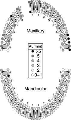
Figure 1: Observed CAL for a typical patient. The shaded boxes represent teeth, the circles represent measurement sites, and the gray lines represent neighbor pairs connecting adjacent sites on the same tooth and sites that share a gap between teeth. “Maxillary” and “Mandibular” refer to upper and lower jaws respectively. The small numbers beside each tooth are the “tooth numbers.” The maxilla’s second tooth on the left is missing; third molars (“wisdom teeth”) are excluded.

The motivating example is a clinical study conducted at the Medical University of South Carolina (MUSC) to determine the periodontal disease status for Type-2 diabetic Gullah-speaking African-Americans, originally presented in Fernandez et al. (2009). The objective of this analysis is to quantify the disease status of this population, and to study the associations between disease status and patient-level covariates such as age, BMI, gender, HbA1C and smoking status.

Quantifying a patient’s disease status from the extensive data collected during a periodontal exam is difficult. For example, it is common to summarize disease status using the whole-mouth average CAL or the number of teeth with CAL above a certain threshold. Using the whole-mouth average CAL as the response in a regression with patient-level covariates is reasonable when the patients’ residual distributions are identical. However, this assumption is often violated in practice, as different patients have different error variances, spatial covariances and missing data patterns. In this paper we present a multivariate spatial model to jointly analyze periodontal data from multiple markers and multiple measurement locations to improve estimation of disease status, and hence develop a more powerful method for studying the association between patient-level covariates and periodontal disease.

We use spatial factor analysis [Wang and Wall (2003), Hogan and Tchernis (2004), Lopes, Salazar and Gamerman (2008)] to model these multivariate spatial data. We postulate that the three markers are all related to a single latent spatial process (factor) measuring periodontal health. The latent periodontal health factor varies from site to site and is smoothed spatially using a conditionally autoregressive prior [Besag, York and Mollié (1991), Banerjee, Carlin and Gelfand (2004)]. The data collected for this study provide interesting challenges that require extensions of the spatial factor model. First, the data are a mix of continuous and binary responses. To jointly model these data types, we develop a spatial probit model for binary responses, which has the advantage of being fully-conjugate and leads to rapid MCMC sampling and convergence. Also, we have data from multiple patients, and exploratory analysis suggests that the covariance of the latent spatial factor varies by patient. Therefore, we develop a hierarchial model which allows the covariance to vary between patients, but pools information across patients to estimate the covariance parameters. We show in a simple case that in terms of estimating the effect of patient-level covariates, this model is equivalent to a weighted multiple regression, where the patient’s scalar response is a linear combination of all data across location and marker, and the patient’s weight decreases with the spatial correlation and variability.

Another challenging aspect of analyzing periodontal data is the considerable number of missing teeth (around 20% for these data). The assumption that teeth are missing completely at random is not valid because periodontal disease is the leading cause of adult tooth loss, so patients with several missing teeth likely have poor periodontal health. For nonspatial data a common method to handle so-called “informative cluster size” is to include the number of observations as a covariate, or in the weights of a weighted regression [Hoffman, Sen and Weinberg (2001), Williamson, Datta and Satten (2003), Follman, Proschan and Leifer (2003), Lu (2005), Benhin, Rao and Scott (2005), Panageas et al. (2007), Cong, Yin and Shen (2007), Williamson et al. (2008)]. Dunson, Chen and Harry (2003) take a different approach. They propose a joint model for clustered mixed (continuous and binary) data and the number of responses in each cluster, using a continuation ratio probit model for cluster size. Another approach is the shared parameter model [e.g., Wu and Carroll (1988), Follman and Wu (1995)]. The shared parameter model accounts for informative missingness by introducing random effects that are shared between the missing data process and the measurement process. Conditioned on the random effects, the missing data and measurement processes are assumed to be independent.

We propose a shared variable model to jointly model missing teeth with the other markers of periodontal disease. However, in our spatial setting both the number and location of missing teeth are informative. For example, a missing tooth in the front of the mouth surrounded by teeth with low CAL may not be informative; in contrast, a missing tooth in the back of the mouth (where periodontal disease is often the most advanced) surrounded by teeth with high CAL is indicative of poor periodontal health in that region of the mouth. Therefore, we model the number and spatial distribution of missing teeth using our latent spatial factor model. In this model, CAL, PPD, BOP and the location of missing teeth are all modeled simultaneously in terms of a latent periodontal health factor; this approach uses all available information to estimate periodontal disease status.

The paper proceeds as follows. Section 2 presents our unified approach to modeling multivariate spatially-referenced periodontal data, as well as our model for informatively missing teeth. Section 3 offers some influence diagnostics to determine which patients and response types are the most informative about the patient-level covariates. Computing details are given in Section 4. Section 5’s simulation study shows that accounting for spatial association and informative observation location can lead to a substantial improvement in estimating the patient-level covariate effects. We analyze the periodontal data in Section 6. Section 7 concludes.

2 Latent spatial factor model for periodontal data

In this section we describe our approach for spatially-referenced mixed periodontal data with informative missingness. We begin in Section 2.1 by specifying a latent spatial factor model assuming no missing teeth. Section 2.2 introduces the spatial probit model for missing teeth and Section 2.3 specifies priors and discusses identifiability of the latent variable model.

2.1 Complete data model

We assume our multivariate spatial data has $J$ types of responses (for the periodontal data the $J=3$ responses are CAL, PPD and BOP) at each spatial location for each patient. If the $j$th type of response is continuous (CAL and PPD), let $y_{ij}(s)$ be the response at spatial location $s$ for patient $i$, $s=1,\ldots,S$ and $i=1,\ldots,N$. Our data also has binary responses (BOP). If the $j$th type of response is binary, let $y^{*}_{ij}(s)$ be the response at spatial location $s$ for patient $i$. We model binary responses using probit regression, that is, $y^{*}_{ij}(s)=I(y_{ij}(s)>0)$, where $I(\cdot)$ is the binary indicator function and $y_{ij}(s)$ is a Gaussian latent variable.

All $J$ responses are modeled as functions of the latent spatial disease status, $\mu_{i}(s)$, which represents the overall periodontal health of patient $i$ at location $s$. Let

$$y_{ij}(s)=a_{j}+b_{j}\mu_{i}(s)+\varepsilon_{ij}(s),$$ (1)

where $a_{j}$ is the intercept for response $j$, $b_{j}$ relates the latent factor to response type $j$, and $\varepsilon_{ij}(s)\sim$ $N(0,\sigma_{ij}^{2}$) is error. As is customary for probit regression, we assume $\sigma_{ij}^{2}=1$ for binary responses for identification. Since all $J$ responses depend on the common latent factor, they are correlated with

$$\operatorname{Cor}(y_{ij}(s),y_{il}(s))=\frac{b_{j}b_{l}\operatorname{Var}[\mu_{i}(s)]}{\sqrt{b_{j}^{2}\operatorname{Var}[\mu_{i}(s)]+\sigma^{2}_{ij}}\sqrt{b_{l}^{2}\operatorname{Var}[\mu_{i}(s)]+\sigma^{2}_{il}}}.$$ (2)

The slopes $b_{j}$ and $b_{l}$ determine the sign and magnitude of the correlation; if either $b_{j}$ or $b_{l}$ is zero, then $y_{ij}(s)$ and $y_{il}(s)$ are uncorrelated, and if $b_{j}$ and $b_{l}$ share (do not share) the same sign, then $y_{ij}(s)$ and $y_{il}(s)$ are positively (negatively) correlated.

The latent vector $\bolds{\mu}_{i}=(\mu_{i}(1),\ldots,\mu_{i}(S))^{\prime}$ has a multivariate normal prior with conditionally autoregressive covariance [“CAR,” Besag, York and Mollié (1991)]. The mean of $\bolds{\mu}_{i}$ is

$$E(\bolds{\mu}_{i})=W\bolds{\alpha}+\Omega_{i}\bolds{\beta},$$

where $W$ is an $S\times q$ matrix of spatial covariates (e.g., tooth number) that do not vary across patient, $\mathbf{X}_{i}$ is the $p$-vector of patient-level covariates (e.g., age) that do not vary across space within patient, $\Omega_{i}=X_{i}^{\prime}\otimes\mathbf{1}_{S}$, $\mathbf{1}_{S}$ is the $S$-vector of ones, and $\bolds{\alpha}$ and $\bolds{\beta}$ are the corresponding regression parameters. The covariance of $\bolds{\mu}_{i}$ is $\tau_{i}^{2}Q(\rho_{i})^{-1}$, where $Q(\rho_{i})=M-\rho_{i}D$, $D_{ss^{\prime}}$ is one if locations $s$ and $s^{\prime}$ are adjacent and zero otherwise, $M$ is diagonal with diagonal elements $M_{ss}=\sum_{s^{\prime}}D_{ss^{\prime}}$. In this spatial model, $\rho_{i}\in[0,1]$ controls the degree of spatial association and $\tau_{i}^{2}>0$ controls the magnitude of variation. Let $r_{i}(s)=\mu_{i}(s)-E(\mu_{i}(s))$. A convenient interpretation of the CAR prior is that the conditional distribution of $r_{i}(s)$ given $r_{i}(s^{\prime})$ for all $s^{\prime}\neq s$ is normal with mean $\rho_{i}\bar{r}_{i}(s)$ and variance $\tau_{i}^{2}/m(s)$, where $\bar{r}_{i}(s)$ is the average of $r_{i}(s)$ at location $s$’s $m(s)$ neighbors.

The degree of spatial variation is allowed to differ between patients by means of $\sigma_{ij}^{2}$, $\tau_{i}^{2}$ and $\rho_{i}$. To pool information across patients, we use models

$$\sigma_{ij}^{-2}|c_{j},d_{j} \sim \operatorname{Gamma}(c_{j},d_{j}),$$

$$\tau_{i}^{-2}|e,f \sim \operatorname{Gamma}(e,f),$$ (3)

$$\rho_{i}|g,h \sim \operatorname{Beta}(g,h),$$

where $\{c_{j}\}$, $\{d_{j}\}$, $e$, $f$, $g$ and $h$ are hyperparameters.

2.2 Model for the location of missing teeth

For our data described in Section 1, roughly 20% of the teeth are missing. The locations of the missing teeth are not random, but rather related to the periodontal health in that region of the mouth. Therefore, we propose a model for the location of missing teeth as a function of the underlying latent factor $\mu_{i}(s)$.

For our data either the six observations on a tooth for all $J$ responses are all observed or all unobserved. That is, if a tooth is missing, we have no data for the tooth, and if a tooth is not missing, we have complete data. Let $y^{*}_{i0}(t)$ be an indicator of whether tooth $t=1,\ldots,T$ is missing for patient $i$. As with the binary data in Section 2, we model $y^{*}_{i0}(t)$ using probit regression. Let $y^{*}_{i0}(t)=I(y_{i0}(t)>0)$, where $y_{i0}(t)$ is a latent continuous variable. Then

$$y_{i0}(t)=a_{0}+b_{0}Z_{t}^{\prime}\bolds{\mu}_{i}+\varepsilon_{i0}(t),$$ (4)

where $Z_{t}$ is such that $Z_{t}^{\prime}\bolds{\mu}_{i}$ is the mean of $\bolds{\mu}_{i}$ at the six observations on tooth $t$ and $\varepsilon_{i0}(t)\stackrel{{\scriptstyle\mathrm{i.i.d.}}}{{\sim}}N(0,1)$. $a_{0}$ and $b_{0}$ relate the latent process to the missing tooth indicator. Note that since $\mu_{i}(s)$ is included in both the model for presence of and value of the responses, both presence and value of the data contribute to the posterior of $\mu_{i}(s)$, and thus the posterior of $\bolds{\beta}$. Also note that $b_{i0}=0$ corresponds to independence between the latent factor and the location of missing teeth, in which case the location of missing teeth does not contribute to estimating $\bolds{\beta}$.

2.3 Identifiability and prior choice

Identifiability is a key issue in latent variable modeling. To see this, we inspect the first two moments of the multivariate response at location $s$ for patient $i$ after integrating over the latent factor $\bolds{\mu}_{i}$,

$$\mbox{E}(y_{ij}(s)) = a_{j}+b_{j}[W(s)\bolds{\alpha}+\mathbf{X}_{i}^{\prime}\bolds{\beta}],$$

$$\operatorname{Cov}(y_{ij}(s),y_{il}(s)) = b_{j}b_{l}\tau_{i}^{2}q(s)+I(j=l)\sigma^{2}_{ij},$$

where $W(s)$ is the row of $W$ corresponding to location $s$ and $q(s)$ is the $(s,s)$ diagonal element of $Q(\rho_{i})^{-1}$. Identifiability concerns arise in both moment expressions, as multiplying all of the slopes $b_{j}$ by scalar $c$ and dividing $\bolds{\alpha}$, $\bolds{\beta}$ and $\tau_{i}^{2}$ by $c$ gives identical moments. Although there are other ways to address this issue, we fix $b_{1}\equiv 1$. This identifies both the regression coefficients $\bolds{\alpha}$ and $\bolds{\beta}$ via the mean of the first response and the CAR variance $\tau_{i}^{2}$ via the variance of the first response. In our analysis of periodontal data of Section 6 we take the first response with fixed slope to be clinical attachment loss, the most commonly used measure of periodontal disease. We also compare these results with other baseline assignments and discuss sensitivity to this assumption.

The regression coefficients $\{a_{j}\}$, $\{b_{j}\}$ ($j\neq 1$), $\bolds{\alpha}$ and $\bolds{\beta}$ have independent $N(0,w^{2})$ priors. The hyperparameters $\{c_{j}\}$, $\{d_{j}\}$, $e$, $f$, $g$ and $h$ have independent Gamma($u,v$) priors. In the simulation study (Section 5) and data analysis (Section 6) we take $u=v=0.1$ and $w=10$ to give vague yet proper priors. We conduct a sensitivity analysis in Section 6 which shows that the results are not sensitive to these priors for this large periodontal data set.

3 Influence diagnostics

Our primary interest is in the patient-level parameters $\bolds{\beta}$. In this complicated hierarchical Bayesian model, we would like to identify the sources of data that are most informative about $\bolds{\beta}$. In this section we develop diagnostics to determine which patients, spatial locations and response types are the most influential. We assume no missing teeth, that all responses are Gaussian, and that no covariates depend on space ($W$ is null). In this case the regression coefficients only affect the overall average response for each patient, and a tempting simplification is to collapse data over space and use each patient’s overall average as a scalar response. We show that even in this case different areas of the mouth are more than less informative, and that patients are weighted differently depending on their spatial covariance parameters. This motivates the hierarchical spatial model even in this simple case.

Integrating over latent effect $\bolds{\mu}_{i}$, but conditioning on $\sigma^{2}_{ij}$, $\tau^{2}_{i}$, $\rho_{i}$, $a_{j}$ and $b_{j}$, the posterior for $\bolds{\beta}$ is Gaussian with

$$\operatorname{COV}(\bolds{\beta}) = \Biggl{(}\sum_{i=1}^{N}w_{i}\mathbf{x}_{i}\mathbf{x}_{i}^{\prime}\Biggr{)}^{-1},$$

$$E(\bolds{\beta}) = \Biggl{(}\sum_{i=1}^{N}w_{i}\mathbf{x}_{i}\mathbf{x}_{i}^{\prime}\Biggr{)}^{-1}\sum_{i=1}^{N}w_{i}\mathbf{x}_{i}^{\prime}z_{i},$$

where

$$w_{i}=\tau_{i}^{-2}\mathbf{1}^{\prime}\bigl{[}Q(\rho_{i})-Q(\rho_{i})\bigl{(}\delta_{i}I_{S}+Q(\rho_{i})\bigr{)}^{-1}Q(\rho_{i})\bigr{]}\mathbf{1},$$ (7)

$\delta_{i}=\tau_{i}^{2}\sum_{j=1}^{J}b_{j}^{2}/\sigma_{ij}^{2}$, and

$$z_{i}=\frac{1}{w_{i}}\mathbf{1}^{\prime}Q(\rho_{i})\bigl{(}\delta_{i}I_{s}+Q(\rho_{i})\bigr{)}^{-1}\sum_{j=1}^{J}b_{j}\sigma_{ij}^{-2}(\mathbf{y}_{ij}-a_{j}).$$

The posterior in (3) is equivalent to a weighted linear regression where each patient contributes the scalar response $z_{i}$ and is weighted according to $w_{i}$. Analyzing $z_{i}$ and $w_{i}$ shows which sites, patients and outcomes contribute the most to $\bolds{\beta}$’s posterior.

First we consider $z_{i}$:

$$z_{i} = \frac{1}{w_{i}}\mathbf{1}^{\prime}\bigl{[}Q(\rho_{i})\bigl{(}\delta_{i}I_{s}+Q(\rho_{i})\bigr{)}^{-1}\bigr{]}\sum_{j=1}^{J}\frac{b_{j}}{\sigma_{ij}^{2}}(\mathbf{y}_{ij}-a_{j})$$

$$= \sum_{j=1}^{J}\frac{b_{j}}{\sigma_{ij}^{2}}\Biggl{[}\sum_{s=1}^{S}k_{i}(s)\bigl{(}y_{ij}(s)-a_{j}\bigr{)}\Biggr{]},$$

where the vector $k_{i}=\mathbf{1}^{\prime}[Q(\rho_{i})(\delta_{i}I_{s}+Q(\rho_{i}))^{-1}]/w_{i}$. Therefore, $z_{i}$ is a linear combination of all the observations for patient $i$, with $k(s)$ controlling the relative weight of observations at location $s$ and $b_{j}/\sigma_{ij}^{2}$ controlling the relative weight of response type $j$. Figure 2(a) plots $k(s)$ (scaled to sum to $S$) for four combinations of $\rho_{i}$ and $\delta_{i}$. Observations in the gaps between teeth have the highest weight; these sites have the most neighbors and thus the smallest prior variance. Observations in the back of the mouth and on the sides of teeth get less weight.

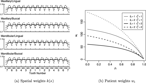
Figure 2: Panel (a) plots the spatial weights $k(s)$ for various $\delta$ and $\rho$. “Maxillary” and “Mandibular” refer to upper and lower jaws respectively, while “buccal” and “lingual” refer to the cheek and the tongue sides of the teeth, respectively. The thin lines have $\rho=0.1$, the wide lines have $\rho=0.99$; the solid lines have $\delta=0.2$, the dashed lines have $\delta=5$. Panel (b) plots the patient weights $w_{i}$ for various $\delta_{i}$, $\tau_{i}$ and $\rho_{i}$.

The patient weights $w_{i}$ are plotted as a function of $\rho_{i}$, $\delta_{i}$ and $\tau_{i}$ in Figure 2(b). The weight decreases with $\rho_{i}$ and $\tau_{i}^{2}$, and increases with $\delta_{i}$ (inversely related to error variances $\sigma_{ij}^{2}$). That is, patients with little spatial association and small variances $\tau_{i}^{2}$ and $\sigma_{ij}^{2}$ (and thus large $\delta_{i}$) have the most influence on $\bolds{\beta}$’s posterior. To search for overly-influential patients, we compute the weights by evaluating (7) using posterior means ${\hat{\rho}}_{i}$, ${\hat{\tau}}_{i}^{2}$ and ${\hat{\sigma}}_{i1}^{2}$. However, the marginal posterior for $\bolds{\beta}$ is not available in closed-form for Section 6’s data with informative missing teeth and binary responses. Therefore, we use only the CAL error variance ${\hat{\sigma}}_{i1}^{2}$, that is, $\delta_{i}={\hat{\tau}}_{i}^{2}/{\hat{\sigma}}_{i1}^{2}$ ($b_{1}=1$, Section 2.3), as an approximation. This approximation is not meant to be definitive, but rather a useful heuristic device.

4 MCMC sampling algorithm

MCMC sampling is carried out using the free software R (http://www.r-project.org/), although it would also be straightforward to implement the model using WinBUGS(http://www.mrc-bsu.cam.ac.uk/bugs/). Sample code to analyze a single continuous response is available in the supplemental article [Reich and Bandyopadhyay (2009)]. We draw 20,000 MCMC samples and discard the first 5000 as burn-in. Convergence is monitored using trace plots of the deviance as well as several representative parameters.

The patient-specific parameters are conditionally-conjugate except for the CAR spatial association parameters $\rho_{i}$, which are updated using Metropolis–Hastings sampling with a Beta$(50\rho_{i}^{*},50(1-\rho_{i}^{*}))$ candidate distribution, where $\rho_{i}^{*}$ is the value at the previous iteration. The remaining parameters are updated using Gibbs sampling with full conditionals given below. The latent continuous variables corresponding to the probit model for binary responses, $y_{ij}(s)$, are updated from their truncated full conditionals $y_{ij}(s)\sim N(a_{j}+b_{j}\mu_{i}(s),1)$, restricted to $(-\infty,0)$ if $y^{*}_{ij}(s)=0$ and $(0,\infty)$ if $y^{*}_{ij}(s)=1$. The vector of latent effects for patient $i$, $\bolds{\mu}_{i}$, is multivariate normal with

$$V(\bolds{\mu}_{i}|\operatorname{rest})^{-1} = \mathbf{Z}^{\prime}\mathbf{Z}b_{0}^{2}+Q(\rho_{i})/\tau_{i}^{2}+\Biggl{(}\sum_{j=1}^{J}b_{j}^{2}/\sigma_{ij}^{2}\Biggr{)}I_{n},$$

$$E(\bolds{\mu}_{i}|\operatorname{rest}) = V(\bolds{\mu}_{i}|\operatorname{rest})\Biggl{(}b_{0}\mathbf{Z}^{\prime}(\mathbf{y}_{0i}-a_{0})$$

$$\hskip 54.0pt{}+Q(\rho_{i})(W\bolds{\alpha}+\Omega_{i}\bolds{\beta})/\tau_{i}^{2}+\sum_{j=1}^{J}b_{j}(\mathbf{y}_{ij}-a_{j})/\sigma_{ij}^{2}\Biggr{)},\vspace*{-1pt}$$

where $\mathbf{Z}=(Z_{1},\ldots,Z_{T})$, $\mathbf{y}_{ij}=(y_{ij}(1),\ldots,y_{ij}(S))$ and $\mathbf{y}_{i0}=(y_{i0}(1),\ldots,\break y_{i0}(T))$. The measurement error variances for the continuous responses have full conditional

$$\hskip 5.0pt\sigma^{2}_{ij}|\operatorname{rest} \sim \operatorname{InvGamma}\Biggl{(}S/2+c_{j},\sum_{s=1}^{S}\bigl{(}y_{ij}(s)-a_{j}-b_{j}\mu_{i}(s)\bigr{)}^{2}/2+d_{j}\Biggr{)},$$

$$\tau^{2}_{j}|\operatorname{rest} \sim \operatorname{InvGamma}\bigl{(}S/2+e,\mathbf{r}_{i}^{\prime}Q(\rho_{i})\mathbf{r}_{i}/2+f\bigr{)},$$

where $\mathbf{r}_{i}=\bolds{\mu}_{i}-W\bolds{\alpha}-\Omega_{i}\bolds{\beta}$.

The intercept/slope pairs $(a_{j},b_{j})$ have bivariate normal full conditionals with mean

$$V((a_{j},b_{j})^{\prime}|\operatorname{rest})^{-1} = w^{-2}I_{2}+\sum_{i=1}^{N}\Delta_{i}^{\prime}\Delta_{i}/\sigma^{2}_{ij},$$

$$E((a_{j},b_{j})^{\prime}|\operatorname{rest}) = V((a_{j},b_{j})^{\prime}|\operatorname{rest})\Biggl{(}\sum_{i=1}^{N}\Delta_{i}^{\prime}\mathbf{y}_{ij}/\sigma^{2}_{ij}\Biggr{)},$$

where $\Delta_{i}=(\mathbf{1},\bolds{\mu}_{i})$. The regression coefficients $\bolds{\alpha}$ and $\bolds{\beta}$ have multivariate normal full conditionals with

$$V(\bolds{\alpha}|\operatorname{rest})^{-1} = w^{-2}I_{p_{s}}+\sum_{i=1}^{N}W^{\prime}Q(\rho_{i})W/\tau^{2}_{i},$$

$$E(\bolds{\alpha}|\operatorname{rest}) = V(\bolds{\beta}_{s}|\operatorname{rest})\mathbf{X}_{s}^{\prime}\sum_{i=1}^{N}Q(\rho_{i})(\bolds{\mu}_{i}-\Omega_{i}^{\prime}\bolds{\beta})/\tau^{2}_{i}$$

and

$$V(\bolds{\beta}|\operatorname{rest})^{-1} = w^{-2}I_{p}+\sum_{i=1}^{N}\Omega_{i}^{\prime}Q(\rho_{i})\Omega_{i}/\tau^{2}_{i},$$

$$E(\bolds{\beta}|\operatorname{rest}) = V(\bolds{\beta}|\operatorname{rest})\sum_{i=1}^{N}\Omega_{i}^{\prime}Q(\rho_{i})(\bolds{\mu}_{i}-W\bolds{\alpha})/\tau^{2}_{i}.$$

The remaining parameters $\{c_{j}\}$, $\{d_{j}\}$, $e$, $f$ and $g$ are updated using Metropolis sampling with Gaussian candidate distributions tuned to give acceptance ratios near 0.40.

5 Simulation study

In this section we conduct a simulation study to demonstrate the effects of spatial correlation and informative missingness on the analysis of patient-level fixed effects. For computational purposes we assume only one quadrant (i.e., half jaw) for each patient leaving $S=42$, that there are no spatial covariates $W$, and the same CAR spatial association parameter for each patient, that is, $\rho_{i}=\rho$. We also assume there is only a single continuous response. Data are generated from the model

$$P\bigl{(}y_{i}(s)=\mbox{observed}\bigr{)} = 1-\Phi\bigl{(}a_{0}+b_{0}\mu_{i}(s)\bigr{)},$$

$$y_{i}(s)|y_{i}(s)\mbox{ observed} \sim N\bigl{(}a_{1}+b_{1}\mu_{i}(s),\sigma_{i}^{2}\bigr{)},$$

where $\bolds{\mu}_{i}\sim N([x_{i}^{\prime}\beta]\mathbf{1}_{S}$, $\tau_{i}^{2}Q^{-1}(\rho)$). Each simulated data set contains data generated from this model for $N=50$ patients. The $p=6$ patient-level covariates $\mathbf{x}_{i}$ are generated independently from the standard normal distribution and the regression coefficients are $\bolds{\beta}=(0,0,0,1,2,3)/20$. Finally, $a_{1}=b_{1}=1$ and $a_{0}=-1$.

$M=100$ data sets are generated from each of six designs specified by varying the true value of the covariance parameters $\sigma_{i}^{2}$, $\tau_{i}^{2}$ and $\rho$ and the missing data mechanism $b_{0}$:

• Design 1: $\rho=0.0$, $b_{0}=0$ and $\sigma_{i}^{2}=\tau_{i}^{2}=1$,

• Design 2: $\rho=0.9$, $b_{0}=0$ and $\sigma_{i}^{2}=\tau_{i}^{2}=1$,

• Design 3: $\rho=0.9$, $b_{0}=0$ and $\sigma_{i}^{2}=\tau_{i}^{2}=$ 1.5*I($i$ is odd)${}+{}$0.5,

• Design 4: $\rho=0.9$, $b_{0}=1$ and $\sigma_{i}^{2}=\tau_{i}^{2}=1$,

• Design 5: $\rho=0.9$, $b_{0}=1$ and $\sigma_{i}^{2}=\tau_{i}^{2}=$ 1.5*I($i$ is odd)${}+{}$0.5,

• Design 6: $\rho=0.5$, $b_{0}=1$ and $\sigma_{i}^{2}=\tau_{i}^{2}=$ 1.5*I($i$ is odd)${}+{}$0.5.

Observations within patients are independent under the first design and spatially correlated under all other designs. The variances are the same for all patients under Design 2 and vary across patients for Design 3. Designs 4 and 5 are similar to Designs 2 and 3, except that the locations of missing observations are informative with $b_{0}=1$. Design 6 is the same as Design 5, except with moderate spatial association $\rho=0.5$.

We analyze each simulated data set using five models:

• Model 1: Linear regression, ${\bar{y}}_{i}=\sum_{s\in S_{i}}y_{i}(s)/|S_{i}|\sim N(x_{i}^{\prime}\beta,\sigma^{2})$,

• Model 2: Section 2’s spatial model without informative missingness or patient-specific variances, that is, $b_{0}=0$, $\sigma_{i}^{2}=\sigma^{2}$ and $\tau_{i}^{2}=\tau^{2}$,

• Model 3: Section 2’s spatial model with patient-specific variances but without informative missingness, that is, $b_{0}=0$,

• Model 4: Section 2’s spatial model with informative missingness but without patient-specific variances, that is, $\sigma_{i}^{2}=\sigma^{2}$ and $\tau_{i}^{2}=\tau^{2}$,

• Model 5: Section 2’s full spatial model,

where $S_{i}$ in Model 1 is the set of locations of observed data for patient $i$. Model 1 ignores spatial associations and missing teeth, and simply uses each patient’s average observed response in a multiple regression. Models 2–5 explicitly model all observations individually and account for spatial associations between nearby observations.

The results are presented in Table 1. For each model and each design, we calculate the proportion of the 95% posterior intervals for $b_{0}$ and the regression coefficients that exclude zero. We also compute the mean squared error and relative bias, $\mathrm{MSE}=\frac{1}{pM}\sum_{m=1}^{M}\sum_{j=1}^{p}(\hat{\beta}_{j}^{(m)}-\beta_{j})^{2}$ and $\mathrm{RelBias}_{j}=\frac{1}{M}\sum_{m=1}^{M}(\hat{\beta}_{j}^{(m)}-\beta_{j})/\beta_{j}$, where $\hat{\beta}_{j}^{(m)}$ is the posterior mean of $\beta_{j}$ for the $m$th simulated data set and $\beta_{j}$ is the true value. Relative bias is only presented for the largest coefficient, $\beta_{6}$.

Table 1: Simulation study results. Column labels “$b_{0}$”–“$\beta_{6}$” give the proportion of 95% intervals that exclude zero. The Monte Carlo standard errors (not shown) are between 0.007 and 0.045 for 100*MSE and between 0.003 and 0.006 for the bias

Design	Model	$\bolds{b_{0}}$	$\bolds{\beta_{1}}$	$\bolds{\beta_{2}}$	$\bolds{\beta_{3}}$	$\bolds{\beta_{4}}$	$\bolds{\beta_{5}}$	$\bolds{\beta_{6}}$	$\bolds{100^{*}\mathrm{MSE}}$	$\bolds{\mathrm{RelBias}_{6}}$
1	1	–	0.06	0.05	0.03	0.29	0.85	1.00	0.103	$0.022$
	2	–	0.05	0.07	0.04	0.34	0.86	1.00	0.103	$0.021$
	3	–	0.05	0.06	0.04	0.35	0.86	1.00	0.104	$0.022$
	4	0.10	0.05	0.05	0.03	0.35	0.85	1.00	0.104	$-0.001$
	5	0.12	0.06	0.05	0.04	0.35	0.83	1.00	0.106	$0.006$
2	1	–	0.03	0.04	0.01	0.13	0.52	0.80	0.289	$0.042$
	2	–	0.03	0.05	0.02	0.15	0.56	0.80	0.287	$0.034$
	3	–	0.03	0.03	0.03	0.17	0.48	0.79	0.298	$0.045$
	4	0.06	0.03	0.06	0.01	0.16	0.52	0.83	0.285	$0.037$
	5	0.06	0.03	0.05	0.01	0.16	0.46	0.81	0.297	$0.043$
3	1	–	0.03	0.07	0.04	0.12	0.31	0.51	0.657	$0.077$
	2	–	0.04	0.08	0.08	0.13	0.31	0.52	0.655	$0.072$
	3	–	0.09	0.09	0.07	0.36	0.69	0.95	0.181	$0.027$
	4	0.08	0.03	0.08	0.09	0.12	0.31	0.56	0.653	$0.077$
	5	0.08	0.09	0.12	0.08	0.39	0.68	0.96	0.178	$0.034$
4	1	–	0.04	0.08	0.05	0.14	0.43	0.70	0.266	$-0.150$
	2	–	0.06	0.05	0.07	0.16	0.43	0.76	0.267	$-0.146$
	3	–	0.04	0.06	0.06	0.18	0.42	0.72	0.265	$-0.141$
	4	1.00	0.04	0.10	0.04	0.18	0.58	0.89	0.278	$0.048$
	5	1.00	0.02	0.06	0.05	0.19	0.58	0.86	0.267	$0.026$
5	1	–	0.05	0.04	0.08	0.07	0.19	0.26	0.780	$-0.229$
	2	–	0.11	0.07	0.12	0.15	0.26	0.34	0.725	$-0.217$
	3	–	0.12	0.11	0.18	0.31	0.67	0.89	0.221	$-0.075$
	4	1.00	0.06	0.10	0.09	0.16	0.46	0.71	0.693	$0.187$
	5	1.00	0.06	0.09	0.08	0.29	0.66	0.94	0.193	$0.023$
6	1	–	0.06	0.04	0.07	0.10	0.28	0.47	0.409	$-0.200$
	2	–	0.16	0.11	0.12	0.18	0.43	0.66	0.383	$-0.191$
	3	–	0.07	0.09	0.11	0.45	0.89	1.00	0.086	$-0.062$
	4	1.00	0.09	0.07	0.11	0.30	0.76	0.97	0.279	$0.130$
	5	1.00	0.06	0.07	0.08	0.61	0.96	1.00	0.070	$0.024$

Data for the first design are generated without spatial association or informative missingness. In this case all five models give nearly identical results, demonstrating that the spatial models are able to approximate the simple regression model if appropriate. The five models are also nearly identical for Design 2 where the data are generated with spatial correlation and the same variances for each patient. In this case the patient means ${\bar{y}}_{i}$ are Gaussian with mean $a_{1}+x_{i}^{\prime}\beta$ and the same variances, satisfying the usual regression assumptions.

The linear regression model does not perform well for Design 3’s spatial model with patient-dependent variances. In this case the patient means ${\bar{y}}_{i}$ have different variances, violating the usual regression assumptions. The spatial models that allow for patient-dependent variances (Models 3 and 5) give dramatic improvements in both power and mean squared error compared to the homoskedastic models.

The locations of missing observations are informative for Designs 4, 5 and 6. For these two designs the models (Models 1–3) that do not account for informative missingness are biased for $\beta_{6}$. The models that allow for informative location consistently identify $b_{0}$ as nonzero (power 1.0 in all three designs), which alleviates the bias for the nonnull predictors and improves power. Design 5 has both informative missingness and patient-dependent variances, common traits of periodontal data. In this case our full model is more than three times more powerful for $\beta_{6}$ (0.26 to 0.94) and has roughly one fourth the mean squared error (0.193 to 0.780) of the usual nonspatial regression approach.

6 Analysis of periodontal data

Table 2: Posterior 95% intervals for models assuming variances $\sigma_{ij}^{2}$ and $\tau_{i}^{2}$ are constant across patients. “Spatial” models take $\rho\neq 0$ and models with informative missing teeth (“Info missing”) have $b_{0}\neq 0$

Spatial	No	No	Yes	Yes
Info missing	No	Yes	No	Yes
Age	($-$0.002, 0.022)	(0.009, 0.033)	(0.000, 0.079)	(0.036, 0.115)
Female	($-$0.129, $-$0.104)	($-$0.128, $-$0.103)	($-$0.181, $-$0.103)	($-$0.173, $-$0.096)
BMI	($-$0.016, 0.007)	($-$0.014, 0.011)	($-$0.048, 0.030)	($-$0.033, 0.046)
Smoker	(0.028, 0.051)	(0.028, 0.051)	(0.014, 0.091)	(0.010, 0.088)
Hba1c	(0.114, 0.139)	(0.118, 0.143)	(0.123, 0.199)	(0.128, 0.207)
$a_{0}$: missing	–	($-$1.390, $-$1.239)	–	($-$1.349, $-$1.172)
$a_{1}$: CAL	(1.008, 1.052)	(1.021, 1.087)	(0.993, 1.112)	(1.002, 1.139)
$a_{2}$: PPD	(1.015, 1.055)	(1.034, 1.101)	(1.092, 1.214)	(1.104, 1.139)
$a_{3}$: BOP	($-$0.369, $-$0.323)	($-$0.359, $-$0.312)	($-$0.399, $-$0.327)	($-$0.394, $-$0.309)
$b_{0}$: missing	–	(0.432, 0.513)	–	(0.434, 0.544)
$b_{2}$: PPD	(1.144, 1.178)	(1.131, 1.160)	(1.021, 1.047)	(1.014, 1.043)
$b_{3}$: BOP	(0.473, 0.510)	(0.475, 0.510)	(0.510, 0.547)	(0.434, 0.544)
$\rho$	–	–	(0.972, 0.978)	(0.972, 0.978)
$\tau$	(1.454, 1.499)	(1.464, 1.508)	(0.832, 0.870)	(0.838, 0.874)
$\sigma_{1}$: CAL	(0.942, 0.961)	(0.972, 0.978)	(0.881, 0.900)	(0.935, 0.953)
$\sigma_{2}$: PPD	(0.106, 0.182)	(0.177, 0.219)	(0.454, 0.486)	(0.464, 0.493)
Tooth 2	($-$0.027, 0.038)	($-$0.038, 0.034)	($-$0.063, 0.027)	($-$0.072, 0.022)
Tooth 3	(0.037, 0.101)	(0.022, 0.091)	($-$0.007, 0.106)	($-$0.025, 0.100)
Tooth 4	(0.174, 0.241)	(0.179, 0.253)	(0.106, 0.242)	(0.138, 0.275)
Tooth 5	(0.237, 0.306)	(0.263, 0.339)	(0.214, 0.369)	(0.296, 0.451)
Tooth 6	(0.751, 0.825)	(0.849, 0.932)	(0.597, 0.773)	(0.853, 1.037)
Tooth 7	(0.866, 0.954)	(0.955, 1.048)	(0.597, 0.773)	(0.986, 1.151)
Gap	(0.953, 1.001)	(0.938, 0.994)	(0.992, 1.030)	(0.986, 1.022)
Maxilla	($-$0.289, $-$0.246)	($-$0.293, $-$0.247)	($-$0.376, $-$0.235)	($-$0.363, $-$0.211)

The motivating data were collected from a clinical study [Fernandes et al. (2009)] conducted by the Center for Oral Health Research (COHR) at the Medical University of South Carolina (MUSC). The relationship between periodontal disease and diabetes level has been previously studied in the dental literature [Faria-Almeida, Navarro and Bascones (2006), Taylor and Borgnakke (2008)]. The objective of this study was to explore the relationship between periodontal disease and diabetes level (determined by the popular marker HbA1c, or “glycosylated hemoglobin”) in the Type-2 diabetic adult (13 years or older) Gullah-speaking African-American population residing in the coastal sea-islands of South Carolina. Since this is part of an ongoing study, we selected 199 patients with complete covariate information and with at least 50% responses available.

For each patient CAL, PPD and BOP are measured at six locations on each nonmissing tooth, as shown in Figure 1. Additionally, several patient-level covariates were obtained, including age (in years), gender (1${}={}$Female, 0${}={}$Male), body mass index or BMI (in kg$/\mbox{m}^{2}$), smoking status (1${}={}$a smoker, 0${}={}$never) and HbA1c (1${}={}$High, 0${}={}$controlled). We also include spatial covariates for the site in the gap between teeth (1${}={}$in the gap, 0${}={}$on the side of a tooth), jaw (1${}={}$maxilla, 0${}={}$mandible) and six tooth number indictors with the first tooth (front of the mouth, Figure 1) serving as the reference tooth. All covariates are standardized to have mean zero and variance one. The spatial adjacency structure is shown in Figure 1; we consider neighboring sites on the same tooth as well as neighboring sites on the consecutive teeth to be adjacent.

We begin by fitting several models with the same variances for all patients, that is, $\sigma_{ij}^{2}=\sigma_{j}^{2}$, $\tau_{i}^{2}=\tau^{2}$ and $\rho_{i}^{2}=\rho^{2}$. We fit four models by assuming spatial association ($\rho\sim\operatorname{Unif}[0,1]$) and independence ($\rho=0$), and assuming missing teeth are informative ($b_{0}\neq 0$) and not informative $(b_{0}=0)$. Table 2 gives posterior 95% intervals for several parameters. The slopes $b_{j}$ for pocket depth and bleeding on probing (as described in Section 2.3, slope for attachment loss is fixed at one) are significantly positive for all models, suggesting strong positive associations between the three responses. Several covariates are significant for all models, including patient effects gender, smoking status and HbA1c status, indicators of a site in the gap between teeth and a site on the upper jaw, and several tooth number indictors with sites in the back of the mouth having higher mean responses.

The slope relating the latent spatial process with the probability of a missing tooth, $b_{0}$, is also significantly positive. This matches the intuition that patients with poor periodontal health generally have more missing teeth. Figure 3 plots the data and fitted values for a typical patient to illustrate the effects of accounting for informative missing teeth. This plot compares the spatial models with $b_{0}$ set to zero (solid lines) and $b_{0}$ not set to zero (dashed lines). The posterior means [Figure 3(a)–(c)] and credible sets [3(d)] are nearly identical for observations on nonmissing teeth. However, for missing teeth the fitted values for all three responses are larger (worse periodontal health) when accounting for informative observation location.

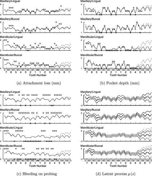
Figure 3: Panels (a)–(c) plot the data (dots) and posterior mean of the expected response (lines) for a typical patient. Panel (d) plots the posterior mean (bold) and 95% interval (thin) for the latent spatial process $\bolds{\mu}(s)$. All plots include results for both the model with (dashed line) and without (solid line) informative observation location. “Maxillary” and “Mandibular” refer to upper and lower jaws respectively, while “buccal” and “lingual” refer to the cheek and the tongue sides of the teeth, respectively.

Accounting for informative observation location also affects the patient effect for age. The 95% interval ignoring spatial association and informative observations location is ($-$0.002, 0.022), compared to (0.036, 0.115) for the full model. The measures of periodontal disease are cumulative, so it seems reasonable that age should be an important predictor. Our data show a relationship between age and the number of missing teeth; patients that are younger than 54 (the mean age) have an average of 135.8 ($\mathrm{sd}=20.1$) observations and patients that are older than 54 have an average of 124.7 ($\mathrm{sd}=22.2$) observations. By accounting for this relationship, we identify age as a significant predictor of periodontal health.

Section 5’s simulation study shows that the fixed effects can also be affected if patients have different spatial covariances. To explore this possibility for our periodontal data, we apply Section 2’s model with variances $\sigma_{ij}^{2}$ and $\tau_{i}^{2}$ varying across patients. Figure 4(a) and (b) summarize the posteriors of the variance parameters. Here we see considerable variation across patients; Figure 4(b) shows that the posterior 95% intervals for $\tau_{i}$ are nonoverlapping for patients with small and large $\tau_{i}$.

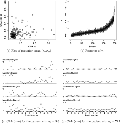
Figure 4: Panel (a) gives the posterior medians of the patient-specific standard deviations $(\tau_{i},\sigma_{ij})$ for attachment loss, and panel (b) plots the posterior of the CAR standard deviations $\tau_{i}$ (the horizontal lines in the $i$th column are the posterior 0.025, 0.25, 0.5, 0.75 and 0.975 quantiles for $\tau_{i}$). Panels (c) and (d) plot the attachment loss for the patients with smallest and largest weights $w_{i}$, respectively. “Maxillary” and “Mandibular” refer to upper and lower jaws, respectively, while “buccal” and “lingual” refer to the cheek and the tongue sides of the teeth, respectively.

Section 3’s $w_{i}$ diagnostic in (7) indicates which patients are the most influential on the regression coefficients. The $w_{i}$ (computed using only the CAL error variance) have median 28.0 and vary greatly across patients with 95% interval (5.8, 61.7). Figure 4(c) and (d) plot CAL for the patients with the smallest and largest $w_{i}$. The responses for the patient with smallest $w_{i}$ vary considerably from site-to-site within the mouth, with attachment loss ranging from 0 to 11 mm. Information about the patient-level covariates accumulate via the mean of the latent parameters $\bolds{\mu}_{i}$; due to spatial variability, the mean is quite uncertain for this patient and, thus, this patient provides little information about $\bolds{\beta}$. In contrast, the patient with largest $w_{i}$ is stable from site-to-site, providing reliable information the mean of $\bolds{\mu}_{i}$ and thus about $\bolds{\beta}$.

Table 3 gives the 95% posterior intervals for several parameters from the model with patient-dependent variances. Comparing the spatial models with informative missingess, the results for the patient-level covariates are fairly similar for the models with and without patient-dependent variances (i.e., the final columns of Tables 2 and 3). However, we note that the width of the credible intervals are smaller for the model with patient-dependent variances.

Table 3: Posterior 95% intervals for models assuming variances $\sigma_{ij}^{2}$ and $\tau_{i}^{2}$ vary across patients. “Spatial” models take $\rho\neq 0$ and models with informative missing teeth (“Info missing”) have $b_{0}\neq 0$

Spatial	No	No	Yes	Yes
Info missing	No	Yes	No	Yes
Age	($-$0.019, 0.007)	($-$0.013, 0.013)	($-$0.002, 0.057)	(0.023, 0.086)
Female	($-$0.114, $-$0.086)	($-$0.115, $-$0.087)	($-$0.159, $-$0.096)	($-$0.168, $-$0.104)
BMI	($-$0.008, 0.019)	($-$0.006, 0.020)	($-$0.015, 0.040)	($-$0.009, 0.050)
Smoker	(0.038, 0.062)	(0.037, 0.061)	(0.021, 0.078)	(0.019, 0.075)
Hba1c	(0.089, 0.114)	(0.090, 0.118)	(0.095, 0.155)	(0.106, 0.171)
$a_{0}$: missing	–	($-$1.154, $-$1.004)	–	($-$1.201, $-$1.040)
$a_{1}$: CAL	(0.859, 0.921)	(0.851, 0.930)	(0.855, 0.942)	(0.892, 0.989)
$a_{2}$: PPD	(0.899, 0.960)	(0.889, 0.966)	(0.920, 1.012)	(0.958, 1.058)
$a_{3}$: BOP	($-$0.425, $-$0.373)	($-$0.424, $-$0.370)	($-$0.482, $-$0.414)	($-$0.464, $-$0.394)
$b_{0}$: missing	–	(0.265, 0.378)	–	(0.294, 0.410)
$b_{2}$: PPD	(1.002, 1.014)	(1.001, 1.014)	(1.017, 1.036)	(1.013, 1.031)
$b_{3}$: BOP	(0.462, 0.499)	(0.463, 0.498)	(0.518, 0.559)	(0.521, 0.560)
$\rho$	–	–	(0.954, 0.962)	(0.958, 0.965)
Tooth 2	($-$0.051, 0.010)	($-$0.050, 0.019)	($-$0.054, 0.023)	($-$0.063, 0.016)
Tooth 3	(0.022, 0.081)	(0.021, 0.086)	(0.007, 0.105)	($-$0.009, 0.095)
Tooth 4	(0.183, 0.246)	(0.190, 0.258)	(0.138, 0.251)	(0.141, 0.254)
Tooth 5	(0.307, 0.374)	(0.318, 0.391)	(0.267, 0.385)	(0.291, 0.412)
Tooth 6	(0.776, 0.850)	(0.825, 0.909)	(0.634, 0.763)	(0.753, 0.899)
Tooth 7	(0.854, 0.940)	(0.902, 0.991)	(0.630, 0.769)	(0.782, 0.938)
Gap	(0.887, 0.929)	(0.886, 0.932)	(0.894, 0.926)	(0.890, 0.922)
Maxilla	($-$0.280, $-$0.241)	($-$0.278, $-$0.238)	($-$0.305, $-$0.208)	($-$0.301, $-$0.201)

Finally, we conducted a sensitivity analysis to determine the effect of modeling assumptions for the full spatial model with patient-dependent variances and informative observation location. We modified the analysis by changing the reference group with slope $b_{j}$ fixed to one from CAL to PPD and BOP, changing the hyperparameters $u=v=0.1$ to $u=v=0.0001$, and changing the hyperparameter $w=10$ to $w=1000$. The posterior 95% intervals are given in Table 4 for the patient effects, scaled by $b_{1}$ for comparison across reference group. The modification with the largest effect is changing the reference group from CAL to BOP. The patient level effects are generally closer to zero using BOP as the reference group. Despite this change in scale, the signs of the coefficients and the subset of coefficients with intervals that exclude zero remains the same as the original analysis.

Table 4: Posterior 95% intervals for the patient effects for various modeling/prior choices for the full model with spatial correlation, patient dependent variance and informative observation location. “Ref group” refers to the response that has slope $b_{j}$ fixed to one, “$u,v$” and “$w$” are the hyperparameters for the covariance parameters and regression coefficients, respectively, as described in Section 2.3. To facilitate comparison across reference groups, the intervals for $\bolds{\beta}/b_{1}$ are presented

Ref group	CAL	PPD	BOP	CAL
$\bolds{u,v}$	$\bolds{0.1}$	$\bolds{0.1}$	$\bolds{0.1}$	$\bolds{0.001}$
$\bolds{w}$	$\bolds{10}$	$\bolds{10}$	$\bolds{10}$	$\bolds{10}$
Spatial grid	$\bolds{1}$	$\bolds{1}$	$\bolds{1}$	$\bolds{1}$
Age	(0.023, 0.086)	(0.025, 0.088)	(0.007, 0.079)	(0.039, 0.110)
Female	($-$0.168, $-$0.104)	($-$0.175, $-$0.108)	($-$0.052, $-$0.031)	($-$0.169, $-$0.097)
BMI	($-$0.009, 0.050)	($-$0.012, 0.052)	($-$0.003, 0.015)	($-$0.015, 0.054)
Smoker	(0.019, 0.075)	(0.020, 0.077)	(0.005, 0.023)	(0.009, 0.075)
Hba1c	(0.106, 0.171)	(0.110, 0.174)	(0.033, 0.054)	(0.122, 0.190)
Ref group	CAL	CAL	CAL
$\bolds{u,v}$	$\bolds{0.1}$	$\bolds{0.1}$	$\bolds{0.1}$
$\bolds{w}$	$\bolds{1000}$	$\bolds{10}$	$\bolds{10}$
Spatial grid	$\bolds{1}$	$\bolds{2}$	$\bolds{3}$
Age	(0.039, 0.109)	(0.023, 0.068)	(0.038, 0.105)
Female	($-$0.174, $-$0.096)	($-$0.150, $-$0.103)	($-$0.167, $-$0.097)
BMI	($-$0.017, 0.050)	($-$0.009, 0.035)	($-$0.011, 0.054)
Smoker	(0.009, 0.076)	(0.024, 0.067)	(0.010, 0.074)
Hba1c	(0.119, 0.191)	(0.117, 0.164)	(0.111, 0.176)

Also, we consider modifying the adjacency structure shown by the gray lines in Figure 1 (“spatial grid 1”) in two ways: first by not considering sites on the opposite side of a tooth to be neighbors (“spatial grid 2”) to give independent $\operatorname{AR}(1)$ models to the sites on the buccal and lingual sides of each jaw, and second by considering all pairs of observations on the same tooth to be neighbors (“spatial grid 3”). To determine how well each of these spatial grids fit our data, we use the deviance information criteria (DIC) of Spiegelhalter et al. (2002). To compare spatial structures using DIC, we analyze only a single continuous response, CAL, and do not consider informative missing teeth. DIC prefers grid 1 (DIC${}={}$66,128) over grids 2 (DIC${}={}$68,168) and 3 (DIC${}={}$68,562). Table 4 gives the posterior of the subject-level effects for the full data analysis using the three spatial grids; the results are not sensitive to the choice of spatial structure.

7 Discussion

In this paper we develop a latent factor model for multivariate spatial periodontal data with a mix of binary and continuous responses. Our model allows for a different spatial covariance for each patient and for informative missing teeth. We show using simulated and real data that accounting for these factors leads to a substantial improvement for estimating covariate effects compared to standard regression techniques.

We have assumed throughout that the patient’s periodontal health can be captured by a single latent factor. It would be straightforward, conceptually if not computationally, to include more latent factors. However, this leads to the problem of selecting the appropriate number of latent factors, interpreting the roles of the different latent factors, and understanding the effects of the covariates on the different latent factors. For these data with three strongly-correlated responses we prefer the single factor model for computational simplicity and interpretability. If multiple factors are allowed, the number of factors could be chosen using the deviance information criteria. Another approach would be to allow the number of factors to be unknown. Lopes, Salazar and Gamerman (2008) and Salazar, Gamerman and Lopes (2009) use reversible jump MCMC to account for uncertainty in the number of latent factors. Extending this approach to our setting may be complicated by the large number of subjects, since the proposal density would have to propose spatial models that simultaneously fit well for all 199 subjects. Another possibility would be to extend the parameter expansion method of Ghosh and Dunson (2008) to the spatial setting.

We have also assumed that the latent spatial process is Gaussian. For nonspatial data several authors have proposed methods that avoid assuming the shared random effects are Gaussian [Lin et al. (2000), Song, Davidian and Tsiatis (2002), Beunckens et al. (2008), Tsonaka, Verbeke and Lesaffre (2009)]. These approaches could be extended to the periodontal setting by replacing the Gaussian spatial model with a non-Gaussian spatial model [e.g., Gelfand, Kottas and MacEachern (2005), Griffin and Steel (2006), Reich and Fuentes (2007)].

An area of future work is to apply this method to longitudinal periodontal data. Periodontal data is often collected repeatedly for a single patient over time to monitor disease progression. Reich and Hodges (2008) propose a spatiotemporal model for attachment loss. It should be possible to extend this model to accommodate mixed multivariate responses and informative missing teeth.

References

- (1) Banerjee, S., Carlin, B. P. and Gelfand, A. E. (2004). Hierarchical Modeling and Analysis for Spatial Data, 1st ed. Chapman & Hall/CRC, Boca Raton, FL.
- (2) Benhin, E., Rao, J. N. K. and Scott, A. J. (2005). Mean estimating equation approach to analysing cluster-correlated data with nonignorable cluster sizes. Biometrika 92 435–450. \MR2201369
- (3) Besag, J., York, J. C. and Mollié, A. (1991). Bayesian image restoration, with two applications in spatial statistics (with discussion). Ann. Inst. Statist. Math. 43 1–59. \MR1105822
- (4) Beunckens, C., Molenberghs, G., Verkeke, G. and Mallinchrodt, C. (2008). A latent-class mixture model for incomplete longitudinal Gaussian data. Biometrics 64 96–105. \MR2422823
- (5) Cong, X. J., Yin, G. and Shen, Y. (2007). Marginal analysis of correlated failure time data with informative cluster sizes. Biometrics 63 663–672. \MR2395702
- (6) Darby, M. L. and Walsh, M. M. (1995). Dental Hygiene: Theory and Practice, 1st ed. W. B. Saunders, Philadelphia, PA.
- (7) Dunson, D. B., Chen, Z. and Harry, J. (2003). A Bayesian approach for joint modeling of cluster size and subunit-specific outcomes. Biometrics 59 521–530. \MR2004257
- (8) Faria-Almeida, R., Navarro, A. and Bascones, A. (2006). Clinical and metabolic changes after conventional treatment of Type-2 diabetic patients with chronic periodontitis. Journal of Periodontology 77 591–598.
- (9) Fernandez, J. K., Wiegand, R. E., Salinas, C. F., Grossi, S. G., Sanders, J. J., Lopes-Virella, M. F. and Slate, E. H. (2009). Periodontal disease status in Gullah African Americans with Type 2 diabetics living in South Carolina. Journal of Periodontology 80 1062–1068.
- (10) Follman, D. and Wu, M. C. (1995). An approximate generalized linear model with random effects and informative missing data. Biometrics 51 151–168. \MR1341233
- (11) Follman, D., Proschan, M. and Leifer, E. (2003). Multiple outputation: Inference for complex clustered data by averaging analyses from independent data. Biometrics 59 420–429. \MR1987409
- (12) Gelfand, A. E., Kottas, A. and MacEachern, S. N. (2005). Bayesian nonparametric spatial modeling with Dirichlet process mixing. J. Amer. Statist. Assoc. 100 1021–1035. \MR2201028
- (13) Ghosh, J. and Dunson, D. B. (2008). Bayesian model selection in factor analytic models. In Random Effect and Latent Variable Model Selection (D. B. Dunson, ed.) 151–164. Wiley, New York.
- (14) Griffin, J. E. and Steel, M. F. J. (2006). Order-based dependent Dirichlet processes. J. Amer. Statist. Assoc. 101 179–194. \MR2268037
- (15) Hoffman, E. B., Sen, P. K. and Weinberg, C. R. (2001). Within-cluster resampling. Biometrika 88 1121–1134. \MR1872223
- (16) Hogan, J. W. and Tchernis, R. (2004). Bayesian factor analysis for spatially correlated data, with application to summarizing area-level material deprivation from census data. J. Amer. Statist. Assoc. 99 314–324. \MR2109313
- (17) Lin, H., McCulloch, C. E., Turnbull, B. W., Slate, E. and Clark, L. (2000). A latent class mixed model for analysing biomarker trajectories with irregularly scheduled observations. Stat. Med. 19 1303–1318.
- (18) Lopes, H. F., Salazar, E. and Gamerman, D. (2008). Spatial dynamic factor analysis. Bayesian Anal. 3 759–792.
- (19) Lu, W. (2005). Marginal regression of multivariate event times based on linear transformation models. Lifetime Data Anal. 11 389–404. \MR2186652
- (20) Oliver, R. C., Brown, L. J. and Loe, H. (1998). Periodontal diseases in the United States population. Journal of Periodontology 69 269–278.
- (21) Panageas, K. S., Schrag, D., Localio, A. R., Venkatraman, E. S. and Begg, C. B. (2007). Properties of analysis methods that account for clustering in volume-outcome studies when the primary predictor is cluster size. Stat. Med. 26 2017–2035. \MR2364289
- (22) Reich, B. J. and Bandyopadhyay, D. (2009). Supplement to “A latent factor model for spatial data with informative missingness.” DOI: 10.1214/09-AOAS278SUPP.
- (23) Reich, B. J. and Fuentes, M. (2007). A multivariate semiparametric Bayesian spatial modeling framework for hurricane surface wind fields. Ann. Appl. Statist. 1 249–264. \MR2393850
- (24) Reich, B. J. and Hodges, J. S. (2008). Modeling longitudinal spatial periodontal data: A spatially-adaptive model with tools for specifying priors and checking fit. Biometrics 64 790–799.
- (25) Salazar, E., Gamerman, D. and Lopes, H. F. (2009). Generalized spatial dynamic factor analysis. Technical report, Univ. Chicago.
- (26) Song, X., Davidian, M. and Tsiatis, A. A. (2002). A semiparametric likelihood approach to joint modeling of longitudinal and time to event data. Biometrics 58 742–753. \MR1945011
- (27) Spiegelhalter, D. J., Best, N. G., Carlin, B. P. and van der Linde, A. (2002). Bayesian measures of model complexity and fit (with discussion). J. Roy. Statist. Soc. Ser. B 64 583–639. \MR1979380
- (28) Taylor, G. W. and Borgnakke, W. S. (2008). Periodontal disease: Associations with diabetes, glycemic control and complications. Oral Diseases 14 191–203.
- (29) Tsonaka, R., Verbeke, G. and Lesaffre, E. (2009). A semi-parametric shared parameter model to handle nonmonotone nonignorable missingness. Biometrics 65 81–87.
- (30) Wang, F. and Wall, M. (2003). Generalized common spatial factor model. Biostatistics 4 569–582.
- (31) Williamson, J. M., Datta, S. and Satten, G. A. (2003). Marginal analysis of clustered data when the cluster size is informative. Biometrics 59 36–42. \MR1978471
- (32) Williamson, J. M., Kim, H. Y., Manatunga, A. and Addiss, D. G. (2008). Modeling survival data with informative cluster size. Stat. Med. 27 543–555. \MR2418464
- (33) Wu, M. C., Carroll, R. (1988). Estimation and comparison of changes in the presence of informative right censoring by modeling the censoring process. Biometrics 44 175–188. \MR0931633