An empirical Bayes mixture method for effect size and false discovery rate estimation

Abstract

Many statistical problems involve data from thousands of parallel cases. Each case has some associated effect size, and most cases will have no effect. It is often important to estimate the effect size and the local or tail-area false discovery rate for each case. Most current methods do this separately, and most are designed for normal data. This paper uses an empirical Bayes mixture model approach to estimate both quantities together for exponential family data. The proposed method yields simple, interpretable models that can still be used nonparametrically. It can also estimate an empirical null and incorporate it fully into the model. The method outperforms existing effect size and false discovery rate estimation procedures in normal data simulations; it nearly acheives the Bayes error for effect size estimation. The method is implemented in an R package (mixfdr), freely available from CRAN.

a1Supported by an NSF VIGRE Fellowship.

Suppose we have $N$ parallel cases, each with some effect size $\delta_{i}$. We observe a measurement $z_{i}\sim f_{\delta_{i}}$ independently for each case. We want to estimate how big each effect is and narrow in on the few cases of interest. To do this, we must estimate $\delta_{i}$ and either the local false discovery rate, $\mathit{fdr}(z)=P(\delta_{i}=0|z_{i})$, or the tail-area false discovery rate, $\mathit{FDR}(z)=P(\delta_{i}=0||z_{i}|\geq z)$. This problem comes up in many different areas: microarrays motivate this paper, but the question also arises in data mining, model selection and image processing [Abramovich et al. (2006), Abramovich, Grinshtein and Pensky (2007), Johnstone and Silverman (2004)].

We present a mixture model empirical Bayes method to solve this problem in Section 1. A simple hierarchical model lets us estimate effect sizes and false discovery rates in a flexible, conceptually neat way. The approach works for general exponential families $f_{\delta}$, and can estimate an empirical null. We illustrate the method for binomial data in Section 2. Simulation results in Section 3 show that the method performs well on normal data: it estimates $\delta$ nearly as well as the Bayes rule, and is a better $\mathit{fdr}$ estimator than existing methods.

1 Model

Our model is a specialization of the Brown–Stein model used by Efron (2008a). This model supposes $(\delta_{i},z_{i})$ are independently generated by the following hierarchical sampling scheme:

$$\delta \sim g(\delta),$$

$$z|\delta \sim f_{\delta}(z),$$

where $f_{\delta}(z)$ is an exponential family with natural parameter $\delta$. Given the prior $g$, we can calculate $\mathit{fdr}(z)$, $\mathit{FDR}(z)$ and the Bayes estimator of $\delta$, $\mathrm{E}(\delta|z)$. However, we usually do not want to specify $g$ in advance. Instead, we can take an empirical Bayes approach: use the data to estimate $g$, and use this estimated prior to get effect size and false discovery rate estimates.

Mixture prior

Modeling $g$ as a mixture gives us the flexibility of a nonparametric model for $g$ with the convenience and stability of a parametric one. We model $g$ as a mixture of $J$ priors $g_{j}$:

$$g(\delta)=\sum_{j=0}^{J-1}\pi_{j}g_{j}(\delta).$$ (1)

The priors $g_{j}$ are taken from some parametric family of priors for $\delta$, and each has a hyperparameter vector $\theta_{j}$. We usually think that the marginal distribution of $z$, $f(z)$, has a known null component $f_{0}$, corresponding to the many cases with $\delta=0$. To model this, we think of the $0$th mixture component as null, and fix $\theta_{0}$ so that $g_{0}$ is a point mass at $0$. The other parameters $\theta_{j}$ and the mixture proportions $\pi_{j}$ are unknown, and must be estimated. We fit them using marginal maximum likelihood via the EM algorithm. We can also incorporate case-specific nuisance parameters into the model as long as they can be estimated. Details for these issues are given in the supplementary information (Muralidharan, 2009).

We can choose any family of priors as long as we can calculate the posteriors, and the family is rich enough to model $g$ nonparametrically given enough components. With such a family, we can go from a strongly parametric model to a nearly nonparametric model by increasing $J$. It is often very convenient to work with conjugate priors for $f_{\delta}$, since the posterior distributions are easy to calculate.

The mixture model gives the posterior distribution of $\delta|z$ a simple form, making it easy to calculate $\mathit{fdr}(z)$ and $\mathrm{E}(\delta|z)$. Let $f^{(j)}=\int f_{\delta}g_{j}(\delta)\,d\delta$ be the $j$th group marginal, so the marginal distribution of $z$ is $f(z)=\sum\pi_{j}f^{(j)}(z)$, and let $F^{(j)}$ and $F$ be corresponding cdfs (the superscripts are to avoid confusion with $f_{\delta}$). Let $p_{j}(z)=\frac{\pi_{j}f^{(j)}(z)}{f(z)}$ be the posterior probability that $z$ came from group $j$, and $g_{j}(\delta|z)$ be the posterior for the $j$th group (that is, the posterior corresponding to prior $g_{j}$). Then under model (1), the posterior distribution is a mixture:

$$\delta|z\sim\sum_{j=0}^{J-1}p_{j}(z)g_{j}(\delta|z).$$ (2)

In particular, this gives us our estimates:

$$\mathit{fdr}(z) = p_{0}(z),$$

$$\mathit{FDR}(z) = \frac{\pi_{0}(1-F^{(0)}(z)+F^{(0)}(-z))}{1-F(z)+F(-z)},$$

$$\mathrm{E}(\delta|z) = \sum_{j=0}^{J-1}p_{j}(z)\mathrm{E}_{j}(\delta|z),$$

where $\mathrm{E}_{j}$ denotes the expectation under $g_{j}(\delta|z)$. Other quantities, like the posterior variance $\operatorname{Var}(\delta|z)$, can be calculated easily using equation 2. These formulas are derived in the supplementary information (Muralidharan, 2009).

Empirical nulls

This model can accommodate empirical nulls by penalizing the mixture proportions and allowing the null component $g_{0}$ to vary. Sometimes, because of correlation or other issues, it is no longer true that most $z\sim f_{0}$ (Efron, 2008b). This makes the theoretical null inappropriate; instead, Efron suggests fitting an empirical null so that most $z$ have the empirical null distribution. In the mixture model, using an empirical null corresponds to $g_{0}$ not being a point mass at $0$ and $\pi_{0}$ being larger than the other $\pi$’s. We can therefore fit an empirical null by letting $g_{0}$ vary and putting a penalty on the proportions $\pi$. The most convenient and interpretable penalty corresponds to a $\operatorname{Dirichlet}(\beta)$ prior on $\pi$. These modifications are easy to incorporate into the fitting process (details are in the supplementary information (Muralidharan, 2009)). Penalizing $\pi$ is useful even for the theoretical null—it stabilizes the parameter estimates by mitigating the effect of the likelihood’s multiple local maxima.

Tuning parameters and how to choose them

This method has two tuning parameters—the penalization parameter $\beta$ and the number of mixture components $J$. Perhaps somewhat counterintuitively, $J$ is less important and easier to choose. This is because for typical datasets, it has little effect on the fitted density $f$, and $\mathrm{E}(\delta|z)$ is a function of $f$ (as Lemma 1 will show). If we treat nearly null components as null (see the next subsection), $\mathit{fdr}$ and $\mathit{FDR}$ estimates are insensitive to $J$ as well. The literature on mixture models has many methods to choose $J$ (McLachlan and Peel, 2000); one easy method is to use the Bayes Information Criterion. For most purposes, however, we can just fix $J$. Taking $J=3$ works particularly well. This choice gives a group each to null, positive effect and negative effect cases.

The penalization $\beta$ can be more important. It is usually best to choose $\beta=(P,0,0,\ldots,0)$. With this choice, the exact value of $P$ is not important for effect size estimation and $\mathit{fdr}/\mathit{FDR}$ estimation with the theoretical null. With empirical nulls, however, $P$ can be more important. A larger $P$ forces a bigger null group, and so increases estimates of the null variance. This can have a big effect on $\mathit{fdr}$ estmates.

We can choose $P$ with a simple parametric bootstrap calibration scheme. First list some candidate penalizations $P_{1},\ldots,P_{K}$ (usually $20$ penalizations evenly spaced between $100$ and $\frac{N}{2}$). Then, fit a preliminary model $m$ to the data using some reasonable default penalization ($P=\frac{1}{5}N$ is a good choice). Next, create perturbed models $m_{1},\ldots,m_{L}$ by changing the null parameters slightly, and possibly changing the alternatives. We will choose $P$ to be the $P_{k}$ that performs best over the perturbed models. To assess performance, generate $B$ random data sets of size $N$ from each $m_{l}$. Fit $k$ mixture models to each bootstrap data set, one for each penalization $P_{k}$, and see how close each of the fitted models is to the true model for that data set (which will be one of the $m_{l}$’s). The best $P$ is the one that performs best over all the bootstrap data sets.

It is worth emphasizing, however, that the mixture model is relatively insensitive to parameter choice. Both $J$ and $P$ have little effect on the fitted density, and so do not affect effect size and theoretical null $\mathit{fdr}/\mathit{FDR}$ estimates too much. This is seen in the simulations of Section 3, where the mixture model nearly acheives the Bayes effect size estimation error for many different combinations of $J$ and $P$.

Choosing a null hypothesis

The mixture model also raises a new question: how should we treat nearly null mixture components? Fitting often gives mixture components that are nearly, but not quite, null. For example, $g_{1}$ might not be a point mass at $0$, but still give $\delta$ close to $0$ with high probability. We need to decide whether to include these components in the null when estimating $\mathit{fdr}$’s and $\mathit{FDR}$’s. Efron (2004) argues that the answer depends on whether the nearly null components are still interesting in the presence of strongly null components. The nearly null components, however, are usually highly sensitive to tuning parameters—different parameters can change the nearly null components dramatically with little effect on the overall density $f$. It is thus usually best to include the nearly null components in the null. If the components are insensitive to parameter choice, though, Efron’s answer is correct, and the question becomes a scientific one.

Identifiability concerns

One problem with this method is that mixture models can be nearly unidentifiable. We can have very different models for $g$ that give nearly the same marginal $f$. We cannot choose between such models based on the data, so estimates of $g$ cannot always be taken seriously. The following result, however, shows that the mean and variance of the posterior distribution $g(\delta|z)$ are simple functions of $f$, and thus can be taken seriously. The result is a generalization of Efron’s calculations in Efron (2008a) to exponential families, though the formula goes back to Robbins (1954). It applies for the Brown–Stein model in general, not just to the mixture model.

Lemma 1

Assume we are in the Brown–Stein model for exponential families and $z$ is continuous. Then the mean and variance of the posterior distribution $g(\delta|z)$ are given by

$$\mathrm{E}(\delta|z) = -\frac{d}{dz}\biggl{(}\log\frac{f_{0}(z)}{f(z)}\biggr{)},$$

$$\operatorname{Var}(\delta|z) = -\frac{d^{2}}{dz^{2}}\biggl{(}\log\frac{f_{0}(z)}{f(z)}\biggr{)}.$$

If we use the theoretical null and $\pi_{0}$ is known, then $\mathit{fdr}(z)=\frac{\pi_{0}f_{0}(z)}{f(z)}$ and $\mathit{FDR}(z)=\frac{\pi_{0}(1-F_{0}(z)+F_{0}(-z))}{1-F(z)+F(-z)}$ are also functions of $f(z)$.

The proof follows (Efron, 2008a) closely. Recall that in the Brown–Stein model we assume only that $\delta$ has prior $g(\delta)$, and $z|\delta\sim f_{\delta}$. The posterior of $\delta|z$ is

$$g_{\delta|z}(\delta) = \frac{f_{\delta}(z)g(\delta)}{f(z)}$$

$$= \exp\biggl{(}z\delta-\log\frac{f(z)}{f_{0}(z)}\biggr{)}e^{-\psi(\delta)}g(\delta).$$

Thus, $\delta|z$ is distributed according to an exponential family with natural parameter $z$ and cumulant generating function $-\log\frac{f_{0}(z)}{f(z)}$. The cumulants of $\delta|z$ are immediately obtained by differentiating this function. Note that this proof goes through for multiparameter exponential families as well.

Lemma 1 connects effect size and $\mathit{fdr}$ estimation in exponential families, and is thus useful beyond the mixture model—any density (or equivalently, $\mathit{fdr}$) estimation method gives us effect size estimates. Such an approach is even useful for discrete families, where the lemma does not apply. The proof shows that $g_{\delta|z}$ is well defined for $z$ in some convex set that includes the sample space of $z$. The problem in the discrete case is that we only know the value of the cumulant generating function in the sample space, and this is not enough to differentiate. We can, however, estimate the cgf by interpolating the known or estimated values. Differentiating this gives us estimates of $\mathrm{E}(\delta|z)$ and $\operatorname{Var}(\delta|z)$ corresponding to priors whose posterior cgfs are not too wild. This method performs well on simulated binomial and Poisson data despite its somewhat shaky theoretical foundations.

Connections to existing methods

This model differs from most $\mathit{fdr}$ and effect size estimation methods in three important ways. First, it estimates $\mathit{fdr}$’s and effect sizes together, not separately. Second, it incorporates its empirical null estimate into its overall density estimate. Finally, it works in general exponential families, not just for normal data or $p$-values.

That said, this mixture model is closely connected to many existing $\mathit{fdr}$ and effect size estimation procedures. $\mathit{fdr}$ estimation under the theoretical null reduces to estimating $\pi_{0}$ [see, for example, Storey (2002), Cai, Jin and Low (2007), Jin and Cai (2007), Meinshausen and Rice (2006)] and $f$ [examples include Efron (2008b), Strimmer (2008)] since $\mathit{fdr}=\frac{\pi_{0}f_{0}}{f}$ [Efron et al. (2001), Storey (2002)]. In this context, the proposed method corresponds to using a mixture model density estimation method. This approach has been successfully used for normal data [Pan, Lin and Le (2003), McLachlan and Peel (2000)], $p$-values (Allison et al., 2002) and Gamma data (Newton et al., 2004). In particular, our treatment of empirical nulls is similar to that of McLachlan and Peel (2000). The proposed method goes further than these methods by incorporating an empirical null estimate into the density estimate and using the mixture model to estimate effect sizes.

The proposed method is also similar to many effect size estimation procedures. Many effect size estimation methods use a two group mixture model for $g$ and estimate $\delta$ with the posterior mean, median or mode. The model can either be specified in advance or estimated empirically—both approaches can yield theoretically attractive estimators [Johnstone and Silverman (2004), Pensky (2006), Abramovich, Grinshtein and Pensky (2007)]. Our mixture model can be viewed as a particular instance of this general recipe for effect size estimation, adapted to estimate $\mathit{fdr}$’s as well. The model is also closely related to another family of procedures that use density estimates and a normal data version of Lemma 1 to estimate effect sizes [Efron (2008a), Brown (2008)]. For continuous $z$, the proposed method corresponds to using a particular mixture density estimator and the more general Lemma 1 to transform the density estimate to an effect size estimate.

2 Binomial data example

To illustrate the mixture model, we use it to predict Major League Baseball batting averages. The data consist of batting records for Major League Baseball players in the 2005 season. We assume that each player has a true batting average $\delta_{i}$, and that his hit total $H_{i}$ is $\operatorname{Binomial}(N_{i},\delta_{i})$, where $N_{i}$ is the number of at bats. The goal is to estimate each players’ batting average $\delta_{i}$ based on the first half of the season. We restrict our attention to players with at least $11$ at bats in this period (567 players).

Brown’s analysis

Brown (2008) analyzes the data using a normalizing and variance stabilizing transformation. He transforms the data $(H,N)$ to

$$X_{i}=\arcsin\sqrt{\frac{H_{i}+1/4}{N_{i}+1/2}},$$

and the transformed data are approximately normal

$$X_{i} {\dot{\sim}} \mathcaligr{N}\biggl{(}\mu_{i},\frac{1}{4N_{i}}\biggr{)},$$

$$\mu_{i} = \arcsin\sqrt{\delta_{i}}.$$

He estimates $\mu_{i}$ using the following methods:

• The naive estimator, $\hat{\mu}_{i}=X_{i}$.

• The overall mean, $\hat{\mu}_{i}=\bar{X}$.

• A parametric empirical Bayes method that models $\mu_{i}\sim\mathcaligr{N}(\mu,\tau^{2})$. The prior parameters $\mu$ and $\tau$ are fit either by method of moments or maximum likelihood.

• A nonparametric empirical Bayes method. First, Brown estimates the marginal density of each $X_{i}$ with a kernel density estimator (tweaked because of the unequal variances). Then he uses a normal version of Lemma 1 from Brown (1971) to estimate $\mu$.

• The positive part James–Stein estimator.

• A Bayesian estimator that models $\mu_{i}\sim\mathcaligr{N}(\mu,\tau^{2})$, $\mu\sim\operatorname{Unif}(\mathbb{R})$, $\tau^{2}\sim\operatorname{Unif}(0,\break\infty)$.

Finally, Brown estimates the estimation error of these methods using their prediction error on the second half of the season. Let $(\tilde{H}_{i},\tilde{N}_{i})$ be the data for the second half of the season. Brown’s error criterion is

$$\mathit{TSE}=\sum(\hat{\mu}_{i}-\tilde{X}_{i})^{2}-\frac{1}{4\tilde{N}_{i}}.$$ (3)

By construction, $\mathrm{E}(\mathit{TSE})=\sum(\hat{\mu}_{i}-\mu_{i})^{2}$. The methods are assessed over all players who had at least $11$ at bats in each half of the data (499 players).

Mixture model

We can analyze the data on the original scale using a binomial mixture model. We model the data using the Brown–Stein model [$\delta_{i}\sim g(\delta)$, $H_{i}|\delta_{i}\sim\operatorname{Binomial}(N_{i},\delta_{i})$], and model $g$ as a mixture of Beta distributions

$$g(\delta)=\sum_{j=0}^{J}\pi_{j}\operatorname{Be}(\delta;\alpha_{j},\beta_{j}).$$

This model makes the marginal distribution of $H_{i}$ a mixture of Beta-binomial distributions, $f(H_{i};N_{i})=\sum\pi_{j}f^{(j)}(H_{i};N_{i})$. The conjugate property of the Beta prior makes the posterior distributions simple:

$$g(\delta_{i}|H_{i})=\sum_{j=0}^{J}p_{j}(H_{i})\operatorname{Be}(\delta;\alpha_{j}+H_{i},\beta_{j}+N_{i}),$$

where $p_{j}(H_{i})=\frac{\pi_{j}f^{(j)}(H_{i};N_{i})}{f(H_{i};N_{i})}$. The parameters $\pi$, $\alpha$ and $\beta$ are fitted by marginal maximum likelihood via the EM algorithm (details are in the supplementary information (Muralidharan, 2009)). For easy comparison with Brown’s results, we estimate $\mu_{i}$ by its posterior mean $\mathrm{E}(\arcsin\sqrt{\delta}|z)$.

Results

Table 1 compares the mixture model to Brown’s methods — the mixture model is a good performer, but not the best. It performs about $15\%$ worse than the nonparametric empirical Bayes and James–Stein estimators. Brown observes that the number of at bats is correlated with the batting averages—better batters bat more. This violates all methods’ assumptions, but has a particularly strong effect on the more parametric methods. Splitting the players into pitchers (81 training, 64 test) and nonpitchers (486 training, 435 test) reduces this effect.

Table 1: Estimated estimation accuracy [equation (3)] for the methods. The naive estimator is normalized to have error $1$. Values for all methods except the binomial mixture model are from Brown (2008). The first column gives the errors on the data as a whole (single model), and the next two give errors for pitchers and nonpitchers considered separately. Standard errors range from $0.05$ to $0.2$ on nonpitchers, are higher for pitchers, and are in between for the overall data [Brown (2008)]

	Overall	Pitchers	Nonpitchers
Number of training players	567	81	486
Number of test players	499	64	435
Naive	$1$	$1$	$1$
Group mean	$0.852$	$0.127$	$0.378$
Parametric empirical Bayes (Moments)	$0.593$	$0.129$	$0.387$
Parametric empirical Bayes (ML)	$0.902$	$0.117$	$0.398$
Nonparametric empirical Bayes	$0.508$	$0.212$	$0.372$
Bayesian estimator	$0.884$	$0.128$	$0.391$
James–Stein	$0.525$	$0.164$	$0.359$
Binomial mixture model	0.588	0.156	0.314

The results, also in Table 1, show that splitting makes the mixture model the best performer for nonpitchers and an average performer for pitchers. Splitting also reduces the differences between the methods. Both the nonparametric empirical Bayes estimator and the binomial mixture model do relatively better on nonpitchers than on pitchers. This is probably because the smaller number of pitchers makes it difficult to estimate the marginal density. Simple simulations show that the binomial mixture model is probably truly better than the other methods for nonpitchers, but no firm conclusions can be drawn about the methods’ relative performance on pitchers or the combined data.

The binomial mixture model has advantages beyond possible performance gains. It removes the need for a normalizing and variance stabilizing transformation by working with the original data. It can estimate any function $h(\delta)$, since $\mathrm{E}(h(\delta)|z)$ can be calculated numerically. Finally, the mixture prior can be informative. For example, the estimated prior for nonpitchers was a single $\operatorname{Beta}(302,884)$ distribution, while the estimated pitchers’ prior was a mixture of $\operatorname{Beta}(90,983)$ and $\operatorname{Beta}(219,928)$ distributions. These prior estimates were stable under different choices of $J$ and starting points for the EM algorithm. This could indicate that nonpitchers are about the same across the league, but pitchers come in two different types.

3 Normal data simulations

In this section we shall see that the mixture model performs very well in the important normal case. The mixture model is particularly simple for normal data. We use the Brown–Stein model [$\delta\sim g(\delta)$, $z|\delta\sim\mathcaligr{N}(\delta,1)$] and model the prior $g$ as a normal mixture:

$$g(\delta)=\sum_{j=0}^{J-1}\pi_{j}\varphi(\delta;\mu_{j},\sigma_{j}^{2}),$$

where $\varphi(x;\mu,\sigma^{2})$ is the $\mathcaligr{N}(\mu,\sigma^{2})$ density function. This model makes the marginal $f$ a normal mixture, $f(z)=\sum\pi_{j}\varphi(z;\mu_{j},\sigma_{j}^{2}+1)$. Fixing $\mu_{0}=0$, $\sigma_{0}=0$ corresponds to using a theoretical null, and letting them vary corresponds to using an empirical null. Normality makes the posterior $g(\delta|z)$ simple. It is easy to check that

$$g(\delta|z) = \sum_{j=0}^{J}p_{j}(z)\varphi\biggl{(}\delta;\frac{1}{\sigma_{j}^{2}+1}\mu_{j}+\frac{\sigma_{j}^{2}}{\sigma_{j}^{2}+1}z,\frac{\sigma_{j}^{2}}{\sigma_{j}^{2}+1}\biggr{)},$$

$$\mathit{fdr}(z) = p_{0}(z),$$

$$\mathrm{E}(\delta|z) = \sum p_{j}(z)\biggl{(}\frac{1}{\sigma_{j}^{2}+1}\mu_{j}+\frac{\sigma_{j}^{2}}{\sigma_{j}^{2}+1}z\biggr{)},$$

where $p_{j}(z)=\frac{\pi_{j}\varphi(z;\mu_{j},\sigma_{j}^{2}+1)}{f}$. The parameters $\pi$, $\mu$ and $\sigma$ are estimated by marginal maximum likelihood via the EM algorithm. We used a $\operatorname{Dirichlet}(P,0,\break\ldots,0)$ penalty on $\pi$ to stabilize the model. The normal mixture model approach is implemented in an R package “mixfdr,” available from CRAN and the author’s website.

Effect size estimation

We can investigate the effect size estimation performance of the normal mixture model with simulation closely based on one done by Johnstone and Silverman (2004). We generate $z_{i}\sim\mathcaligr{N}(\delta_{i},1)$, for $i=1,\ldots,N=1000$. The goal is to estimate $\delta_{i}$ based on $z$ and minimize the squared error $\sum(\delta_{i}-\hat{\delta}_{i})^{2}$. $K$ of the $\delta_{i}$ were nonzero. In the one-sided case, the nonzero $\delta_{i}$ were i.i.d. $\operatorname{Unif}(\mu-\frac{1}{2},\mu+\frac{1}{2})$; in the two-sided case, two-thirds of the $\delta_{i}$ were $\operatorname{Unif}(\mu-\frac{1}{2},\mu+\frac{1}{2})$ and one-third were $\operatorname{Unif}(-\mu-\frac{1}{2},-\mu+\frac{1}{2})$. Different values of $K$ and $\mu$ were used to simulate different combinations of sparsity and effect strengths. We will compare the mixture model to the following effect size estimation methods:

• A spline density method used by Efron (2009).

• EBayesThresh, an empirical Bayes approach taken by Johnstone and Silverman (2004).

• SUREShrink, a method based on minimizing Stein’s Unbiased Risk Estimate for thresholding (Donoho and Johnstone, 1995).

• FDR-based thresholding (Abramovich et al., 2006), at threshold $q=0.1$.

• Soft and hard thresholding using the “universal threshold” $\sqrt{2\log N}\approx 3.7$ from Donoho and Johnstone (1994).

All methods use the known variance of $z$, and when applicable, assume a theoretical $\mathcaligr{N}(0,1)$ null. All methods’ tuning parameters were hand-picked for good performance over the simulation scenarios, but none were rigorously optimized (including the mixture model, which used $J=10$ and $P=50$). The whole simulation was repeated $100$ times, and the same random noise was used for each scenario and each method. Code for the simulation, a slightly modified version of the code used by Johnstone and Silverman (2004), is available in the Supplementary Material online.

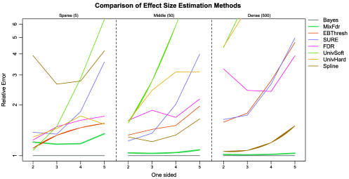
Figure 1: Simulation results for the one-sided scenario. Each panel corresponds to one value of $K$ ($5$, $50$ or $500$). Within each panel, $\mu$ increases from $2$ to $5$. The $y$-axis plots the squared error [$\sum(\delta_{i}-\hat{\delta}_{i})^{2}$], averaged over $100$ replications. Errors are normalized so that the Bayes estimator for each choice of $K$ and $\mu$ has error $1$. Estimation methods are listed in the text. In the dense case, the universal soft and hard thresholding methods are hidden because their relative errors range from $4$ to $40$.

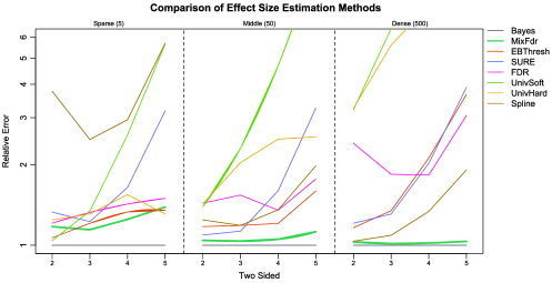
Figure 2: Simulation results for the two-sided scenario. Each panel corresponds to one value of $K$ ($5$, $50$ or $500$). Within each panel, $\mu$ increases from $2$ to $5$. The $y$-axis plots the squared error [$\sum(\delta_{i}-\hat{\delta}_{i})^{2}$], averaged over $100$ replications. Errors are normalized so that the Bayes estimator for each choice of $K$ and $\mu$ has error $1$. Estimation methods are listed in the text. In the dense case, the universal soft and hard thresholding methods are hidden because their relative errors range from $4$ to $50$.

The mixture model was the best performer overall and in most of the cases. Figures 1 and 2 show the performance of the various methods relative to the Bayes estimator for each scenario. The mixture model does a little better than the other methods on sparse $\delta$ ($K=5$) and nearly achieves the Bayes error for moderate and dense $\delta$ ($K=50,500$). Table 2 gives the mean and median relative error over the $24$ scenarios; the mixture model is often within $5\%$ of the Bayes rule, and is the clear winner overall.

=290pt Method Mean Median Mixture Model ($J=10$, $P=50$) 1.10 1.04 Spline 2.08 1.43 EBayesThresh 1.70 1.39 FDR 1.92 1.70 SUREShrink 2.11 1.64 Universal hard 3.60 2.47 Universal soft 8.24 4.52

Table 2: Mean and median relative error for the methods over the simulation scenarios. The relative error is the average of the squared error $\sum(\delta_{i}-\hat{\delta}_{i})^{2}$ over the $100$ replications, divided by the average squared error for the Bayes estimator

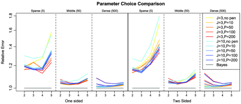
Figure 3: Relative errors for various parameter choices. Each panel corresponds to one value of $K$ ($5$, $50$ or $500$). Within each panel, $\mu$ increases from $2$ to $5$. The $y$-axis plots the squared error [$\sum(\delta_{i}-\hat{\delta}_{i})^{2}$], averaged over $100$ replications. Errors are normalized so that the Bayes estimator for each choice of $K$ and $\mu$ has error $1$. The parameter $J$ gives the number of groups in the mixture model, and $P$ is a penalization parameter.

The mixture model’s performance is not because it is fitting the true model—taking $J$ as low as $3$ gives the same excellent performance (see Figure 3) even though the data are certainly not generated from a three group normal mixture. Neither is its performance due to careful tuning. Performance was insensitive to parameter choice, as Figure 3 shows. The number of groups $J$ does not matter much and as long as there is some penalization, the exact value of $P$ is not too important, especially in the moderate and dense cases.

$\mathit{fdr}$ estimation

We can also investigate the mixture model’s $\mathit{fdr}$ and $\mathit{FDR}$ estimation performance by examining a specific simulation. We generate $z_{i}\sim\mathcaligr{N}(\delta_{i},1)$, $i=1,\ldots,N=1000$. $950$ of the $\delta_{i}$ were $0$. The other $50$ were drawn (once and for all) from a $\operatorname{Unif}(2,4)$ distribution. Various methods were used to estimate the $\mathit{fdr}(z)=P(\delta_{i}\ \mathit{null}|z_{i}=z)$ and $\mathit{FDR}(z)=P(\delta_{i}\ \mathit{null}||z_{i}|\geq z)$ curves based on $z_{i}$, using either theoretical or empirical nulls:

• The normal mixture model with $J=3$ and $P=50$. For this simulation, nearly null components were counted as null.

• Locfdr, from Efron (2008b). This fits the overall density using spline estimation. It fits the empirical null by truncated maximum likelihood (“ML”) or fitting a quadratic to $\log f$ near the center (“CM” for central matching). The implementation in the R package “locfdr” was used.

• Fdrtool, from Strimmer (2008). This fits the overall density using the Grenander density estimator, and the empirical null by truncated maximum likelihood. The implementation in the R package “Fdrtool” was used.

The whole simulation was run $100$ times, and the same random noise was used for each method. The results are similar for other scenarios and parameter choices; the simulation code is available in the Supplementary Information online, and its parameters can be changed easily.

The mixture model is probably the best $\mathit{fdr}$ and $\mathit{FDR}$ estimator, but not by much, and the situation is more complicated than the effect size situation. Figure 4 shows the expectation and standard deviation of $\widehat{\mathit{fdr}}(z)$ for the various methods. Fdrtool’s high bias and variance, and central matching’s high variance, make them poor $\mathit{fdr}$ estimators. This leaves Locfdr (and its ML empirical null method) as the mixture model’s only real competitor. Both methods are nearly unbiased for positive $z$, and their bias for negative $z$ is unlikely to be misleading. The mixture model is slightly more stable than Locfdr, especially in the tails. Results for $\mathit{FDR}$ estimation, seen in Figure 5, were similar.

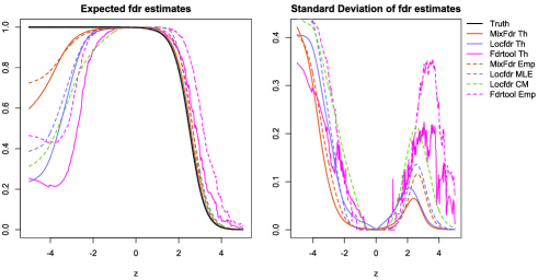
Figure 4: $\mathrm{E}(\hat{\mathit{fdr}}(z))$ and $\operatorname{Sd}(\hat{\mathit{fdr}}(z))$ for various values of $z$ and the methods under consideration. “Th” means the theoretical null was used, while “Emp” means an empirical null was used. Locfdr MLE and CM use the truncated maximum likelihood and central matching empirical null estimates, respectively.

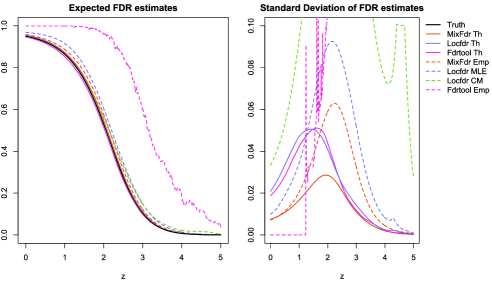
Figure 5: $\mathrm{E}(\hat{\mathit{FDR}}(z))$ and $\operatorname{Sd}(\hat{\mathit{FDR}}(z))$ for various values of $z$ and the methods under consideration. “Th” means the theoretical null was used, while “Emp” means an empirical null was used. Locfdr MLE and CM use the truncated maximum likelihood and central matching empirical null estimates, respectively.

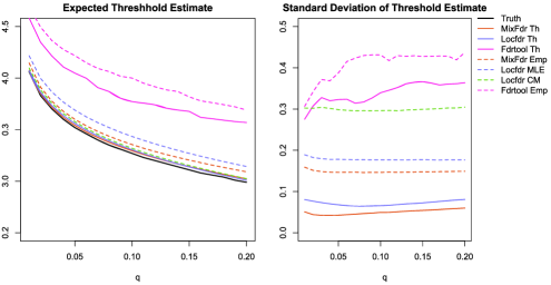
Figure 6: Expectation and standard deviation of rejection threshold estimates $\hat{t}(q)$ for the various methods. The threshholds are $\mathit{fdr}$ based.

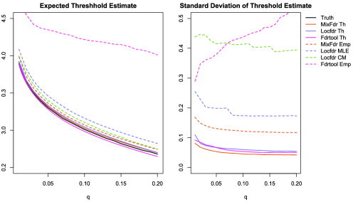
Figure 7: Expectation and standard deviation of rejection threshold estimates $\hat{t}(q)$ for the various methods. The threshholds are $\mathit{FDR}$ based.

The mixture model is nevertheless a little better, especially if we need an empirical null. This is because of the way $\mathit{fdr}$ and $\mathit{FDR}$ estimates are usually used—we typically estimate $\mathit{fdr}(z)$, and use our estimate to find rejection regions $\{z|\mathit{fdr}(z)\leq q\}$. For moderate $q$ ($0.01$ to $0.2$), the rejection regions are in the tails, where the mixture model is stabler. This means that the mixture model is a stabler estimator of the rejection region than Locfdr. In our simulation, the rejection region for a given $q$ corresponds to rejecting all $z$ greater than some threshold $t(q)$. We can use the $\mathit{fdr}$ estimation methods to estimate the rejection thresholds. Figure 6 shows the expectation and standard deviation of $\hat{t}(q)$ for the various methods. Both the mixture model and Locfdr are nearly unbiased for the true threshold, for both theoretical and empirical nulls. Locfdr, however, gives more variable threshold estimates, especially with an empirical null. This makes the mixture model a better choice for threshold estimation. This result held for almost all parameter choices, and is true for $\mathit{FDR}$-based threshholds as well (Figure 7).

4 Summary and extensions

To summarize, the mixture model approach is a simple, flexible and accurate way to estimate $\mathit{fdr}$’s, $\mathit{FDR}$’s and effect sizes. It estimates them together, instead of separately, and can fit an empirical null if required. The method yields simple, interpretable models that can be strongly parametric or quite nonparametric. The method has two tuning parameters—the number of mixture components and the penalization. It is quite insensitive to the first, and, for most purposes, the second. We can choose the penalization by bootstrap calibration. Finally, the method works for exponential families, and can easily accommodate nuisance parameters. It is worth considering a few extensions of the mixture model approach before we close.

The mixture model can be useful even when we are only interested in $\mathit{fdr}$ or $\mathit{FDR}$ estimates. In these situations, the Brown–Stein model imposes unnecessary restrictions on the marginal distribution of the data; it makes sense to drop the model and work with the marginal distribution directly, as much of the $\mathit{fdr}$ literature does [Storey (2002), Efron (2008b)]. The mixture model approach can still be useful in these situations - model the marginal as mixture and penalize the mixture proportions. For example, for normal data, this amounts to modeling the marginal as a normal mixture. This approach can incorporate empirical nulls just as before. The mixture model’s good performance should extend to these approaches.

The mixture model can also be useful beyond exponential families. Section 1 used exponential families for a convenient definition of effect size, for their conjugate priors and for Lemma 1. None of these is central, so if we have data with a natural notion of effect size, we can follow the mixture model’s approach: model the data using a prior on effect sizes, fit a mixture prior by marginal maximum likelihood, then use the Bayes estimates with the estimated prior. The loss of Lemma 1 means that there may be some identifiability issues, but the approach will often still be successful.

References

- Abramovich et al. (2006) Abramovich, F., Benjamini, Y., Donoho, D. L. and Johnston, I. M. (2006). Adapting to unknown sparsity by controlling the false discovery rate. Ann. Statist. 34 584–653. \MR2281879
- Abramovich, Grinshtein and Pensky (2007) Abramovich, F., Grinshtein, V. and Pensky, M. (2007). On optimality of Bayesian testimation in the normal means problem. Ann. Statist. 35 2261–2286. \MR2363971
- Allison et al. (2002) Allison, D. B., Gadbury, G. L., Heo, M., Fernandez, J. R., Lee, C.-K., Prolla, T. A. and Weindruch, R. (2002). A mixture model approach for the analysis of microarray gene expression data. Comput. Statist. Data Anal. 1 1–20. \MR1895555
- Brown (1971) Brown, L. D. (1971). Admissible estimators, recurrent diffusions, and insoluble boundary value problems. Ann. Math. Statist. 42 855–903. \MR0286209
- Brown (2008) Brown, L. D. (2008). In-season prediction of batting averages: A field test of empirical Bayes and Bayes methodologies. Ann. Appl. Statist. 2 113–152. \MR2415597
- Cai, Jin and Low (2007) Cai, T., Jin, J. and Low, M. (2007). Estimation and confidence sets for sparse normal mixtures. Ann. Statist. 35 2421–2449. \MR2382653
- Donoho and Johnstone (1994) Donoho, D. L. and Johnstone, I. M. (1994). Ideal spatial adaptation by wavelet shrinkage. Biometrika 81 425–455. \MR1311089
- Donoho and Johnstone (1995) Donoho, D. L. and Johnstone, I. M. (1995). Adapting to unknown smoothness via wavelet shrinkage. J. Amer. Statist. Assoc. 90 1200–1224. \MR1379464
- Efron (2004) Efron, B. (2004). Large-scale simultaneous hypothesis testing. J. Amer. Statist. Assoc. 99 96–104. \MR2054289
- Efron (2008a) Efron, B. (2008a). Empirical Bayes estimates for large-scale prediction problems.
- Efron (2008b) Efron, B. (2008b). Microarrays, empirical Bayes and the two-groups model. Statist. Sci. 23 1–22. \MR2431866
- Efron (2009) Efron, B. (2009). Correlated -values and the accuracy of large-scale statistical estimates.
- Efron et al. (2001) Efron, B., Tibshirani, R., Storey, J. D. and Tusher, V. (2001). Empirical Bayes analysis of a microarray experiment. J. Amer. Statist. Assoc. 96 1151–1160. \MR1946571
- Jin and Cai (2007) Jin, J. and Cai, T. (2007). Estimating the null and the proportion of non-null effects in large-scale multiple comparisons. J. Amer. Statist. Assoc. 102 495–506. \MR2325113
- Johnstone and Silverman (2004) Johnstone, I. M. and Silverman, B. W. (2004). Needles and straw in haystacks: Empirical Bayes estimates of possibly sparse sequences. Ann. Statist. 4 1594–1649. \MR2089135
- McLachlan and Peel (2000) McLachlan, G. and Peel, D. (2000). Finite Mixture Models. Wiley-Interscience, New York. \MR1789474
- Meinshausen and Rice (2006) Meinshausen, N. and Rice, J. (2006). Estimating the proportion of false null hypotheses among a large number of independently tested hypotheses. Ann. Statist. 34 373–393. \MR2275246
- Muralidharan (2009) Muralidharan, O. (2009). Supplement to “An empirical Bayes mixture method for false discovery rate and effect size estimation”. Ann. Appl. Statist. DOI: 10.1214/09-AOAS276SUPPA, DOI: 10.1214/09-AOAS276SUPPB.
- Newton et al. (2004) Newton, M. A., Noueiry, A., Sarkar, D. and Ahlquis, P. (2004). Detecting differential gene expression with a semiparametric hierarchical mixture method. Biostatistics 5 155–176.
- Pan, Lin and Le (2003) Pan, W., Lin, J. and Le, C. T. (2003). A mixture model approach to detecting differentially expressed genes with microarray data. Functional and Integrative Genomics 3 117–124.
- Pensky (2006) Pensky, M. (2006). Frequentist optimality of Bayesian wavelet shrinkage rules for Gaussian and non-Gaussian noise. Ann. Statist. 34 769–807. \MR2283392
- Robbins (1954) Robbins, H. (1954). An empirical Bayes approach to statistics. In Proc. Thrid Berkeley Sympos. Math. Statist. Probab. 1 (J. Neyman, ed.) 157–163. Univ. California Press, Berkeley, CA. \MR0084919
- Storey (2002) Storey, J. D. (2002). A direct approach to false discovery rates. J. Roy. Statist. Soc. Ser. B 64 479–498. \MR1924302
- Strimmer (2008) Strimmer, K. (2008). A unified approach to false discovery rate estimation. BMC Bioinformatics 9 303.