Pair interactions between complex mesoscopic particles from Widom’s particle-insertion method

Bianca M. Mladek^∗a and Daan Frenkel^a

DOI:10.1039/C0SM00815

We demonstrate that Widom’s particle insertion technique provides a convenient and efficient method to determine the effective pair interaction between complex, composite soft-matter particles in the zero-density limit. By means of three different test systems, i.e. amphiphilic dendrimers, electrostatic polymers and colloids coated with electrostatic polymers, we demonstrate the validity and the power of the presented method.

1 Introduction

Soft materials, be they colloids, polymers or proteins, are often complex constructs that live in a bath of small molecules. In addition, these mesoscopic particles themselves are often composite objects that contain flexible moieties. As a result, atomistic modeling of the structure and dynamics of soft materials would need to span a wide range of length and time scales, which makes such an approach infeasible in all but the simplest cases (few mesoscopic particles and short times).

In an effort to simplify the description of the system at hand, coarse-grained models are being developed that aim to capture the mesoscopic and macroscopic behavior of the system by including in the description only the most relevant degrees of freedom. In the simplest coarse-graining approach each complex, mesoscopic particle is characterized by only one effective coordinate. In the case of particles that have on average inversion symmetry, such as e.g. polymer-coated colloids, this is the coordinate of the center of inversion symmetry. For systems without such symmetry (or, to be more precise, where this symmetry center cannot be identified with a fixed coordinate in the molecular frame) it is conventional to use the center of mass to specify the position of the particle, which is the procedure that is followed for polymers or proteins. The mesoscopic particle is then represented as a “soft” sphere and the effective interaction potential determines the softness. The simplest effective potentials are obtained in the low-density limit where many-body interactions can be ignored. In spite of their simplicity, such models have been shown to work successfully for a range of mesoscopic systems (see e.g.^{1, 2, 3, 4, 5, 6, 7}).

Computing effective interactions for arbitrarily complex mesoscopic particles is one of the key steps in the development of a coarse-grained model. There are many ways in which these interactions can be obtained. The present paper describes an approach that we found to be considerably more efficient than other approaches that we explored.

The paper is organized as follows: in Sec. 2 we define the effective interaction and explain standard Monte Carlo (MC) techniques to determine it, highlighting their strengths and their limitations. In Sec. 3 we adapt Widom’s particle insertion method to the present problem and show that it is an efficient way to determine effective interactions. In Sec. 4 we explain how to implement this formalism and test the method for three different model systems in Sec. 5, comparing the results from the different techniques. In the concluding section (Sec. 6) we point out possible limitations of the method that we present.

2 Computing effective interactions: the standard approach

Consider two mesoscopic particles confined in a volume $V$ and positioned at a distance $R_{12}$ between them. At infinite dilution, the effective pair interaction $\Phi_{\rm eff}(R_{12})$ between these particles is related to their radial distribution function⁸ $g(R_{12})$ via

$$g(R_{12})=\exp\left[-\beta\Phi_{\rm eff}(R_{12})\right],$$ (1)

where $\beta=1/kT$ is the reciprocal temperature^{9, 5}. The radial distribution function, $g(R_{12})$, can easily be measured during the simulation and has to be normalised to 1 for large separations between the particles. Eqn. 1 thus offers a straightforward way to measure the effective interaction within simulations. However, the repulsion between two mesoscopic particles usually increases as the particles approach each other, possibly reaching several $kT$ and configurations where particles are that close are rare. As a result, the relative error in $g(R_{12})$ at short distances will therefore be large, which results in a concomitantly large error in $\Phi_{\rm eff}(R_{12})$. In order to obtain an accurate estimate of $\Phi_{\rm eff}(R_{12})$ without wasting time on irrelevant, though easily accessible configurations, it is therefore necessary to use a simulation technique that samples also the regime where $\Phi_{\rm eff}(R_{12})\gg kT$.

One way to overcome this sampling bottleneck is to sample all relevant values of $R_{12}$ more or less uniformly. Conceptually, the simplest approach to achieve this is to introduce an external biasing potential that acts on the effective coordinates and counteracts the repulsion between the particles. The total interaction is then given by $\tilde{\Phi}(R_{12})=\Phi_{\rm eff}(R_{12})+\Phi_{\rm bias}(R_{12})$ and the radial distribution function is modified to read

$$\tilde{g}(R_{12}) \propto \exp\left[-\beta\tilde{\Phi}(R_{12})\right]$$

$$= \exp\left[-\beta\Phi_{\rm eff}(R_{12})\right]\exp\left[-\beta\Phi_{\rm bias}(R_{12})\right].$$

Comparing this last equation to Eqn. 1, we see that to determine the radial distribution function of the unbiased system, $g(R_{12})$, we have to increment the histogram of the probability of finding the molecules separated by a certain distance $R_{12}$ in each measurement by $\exp\left[\beta\Phi_{\rm bias}(R_{12})\right]$ rather than by 1. The effective interaction can then be determined from this histogram via Eqn. 1.

However, there are two major disadvantages to this approach. First, to sample all relevant distances uniformly, $\tilde{\Phi}(R_{12})$ should be zero (or constant) for all $R_{12}$ and therefore the biasing potential should ideally be $\Phi_{\rm bias}(R_{12})=-\Phi_{\rm eff}(R_{12})$, which would correspond to knowing a priori the sought-after answer. In practice, long simulations are often needed where the biasing potential is determined in a trial-and-error procedure, enhancing the guess for $\Phi_{\rm bias}(R_{12})$ in a rather cumbersome iterative process until the difference to $-\Phi_{\rm eff}(R_{12})$ is smaller than $kT$, which will then allow for an efficient sampling of all distances. But even once the biasing potential is known with sufficient accuracy, sampling will still be slow due to the fact that the mesoscopic particles have to diffuse over the relevant range of $R_{12}$ values to visit each distance often enough.

In an automated process, one can use the Wang-Landau approach¹⁰ to determine the biasing potential and thereby the effective interaction in an iterative way. In this scheme, $g(R_{12})$ is initially unknown and set to unity for all distances $R_{12}$. During the simulation, moves from an old distance $R_{12}^{o}$ with potential energy $U(R_{12}^{o})$ to a new distance $R_{12}^{n}$ with potential energy $U(R_{12}^{n})$ are accepted with a modified Metropolis acceptance rule, where the probability to accept the move is given by

$$P_{\rm acc}(R_{12}^{o}\rightarrow R_{12}^{n})=\min\left[1,e^{-\beta\left[U(R_{12}^{n})-U(R_{12}^{o})\right]}\frac{g(R_{12}^{o})}{g(R_{12}^{n})}\right].$$

In each measurement, the histogram for $g$ at the current position $R_{12}$ is multiplied by a factor $f$, which is usually taken to be 2. At the same time, a histogram of the distances visited is measured and once this histogram is sufficiently flat, a coarse guess for $g(R_{12})$ has been obtained. To refine the results, $f$ is set to $\sqrt{f}$, and the simulation is iterated like this until $f\sim 1$. Then, the effective interaction can be determined via Eqn. 1.

Alternatively, one can break down the range of distances into several small windows^{11, 12} and then use simple biasing potentials to force the system to stay within each window. Typical choices for these so-called umbrella potentials are e.g. hard walls¹³ or spring-like potentials $\Phi_{\rm bias}^{j}(R_{12})=\frac{1}{2}k_{j}(R_{12}-R_{j})^{2}$, where the $k_{j}$ are spring constants that determine the width of each window $j$ located at $R_{j}$. Carrying out separate simulations for the different windows, one can systematically vary the separations between the mesoscopic particles. Within each of these windows $j$, a separate histogram of the probability of finding the molecules a certain distance apart, $g^{j}(R)$, is recorded. At the end of the simulations, the effective potential $\Phi_{\rm eff}(R_{12})$ between the molecules is obtained by merging the effective potentials obtained within each window,

$$\beta\Phi^{j}(R_{12})=-\ln\left[g^{j}(R_{12})\right]-\beta\Phi_{\rm bias}^{j}(R_{12})+c_{j},$$

where $c_{j}$ is a normalization constant. Since the various $c_{j}$ are initially unknown, the concatenation of $\Phi_{\rm eff}(R_{12})$ will display discontinuities at the windows’ edges. To obtain a continuous $\Phi_{\rm eff}(R_{12})$, the $c_{j}$ are chosen such that the data are aligned to each other at the edges of the windows or, more sophisticatedly, the multiple histogram method can be implemented^{14, 15, 12}. Using this umbrella sampling, care has to be taken to choose the windows and umbrella potentials in a way that the variation of the effective interaction within each window does not exceed 1-2 $kT$ to reliably sample the entire window. Moreover, to improve quality of the matching of the different parts of $\Phi_{\rm eff}(R_{12})$ at the edges of the windows, it is advisable to use overlapping windows.

In view of the various limitations of above techniques, it would be desirable to have a straightforward, unbiased method of sampling all distances of approach between two mesoscopic particles with the same probability, while obtaining an efficient estimate of the effective interaction. We show in the next section how Widom’s particle insertion method can be used to achieve precisely this.

3 Formalism

The following formalism is based on Widom’s insertion method to calculate the chemical potential of non-uniform fluids¹⁶. We adapt his approach to determine the effective interactions between two mesoscopic particles in the zero density limit in a fast and straightforward manner. The method presented here is also a generalisation of the scheme used in Ref. 2, where the effective interaction between two self-avoiding, i.e. hard-core, polymers was determined from the overlap probability when placing the polymers random distances apart. Despite this generalisation being straight-forward, we are not aware of earlier implementations.

We consider a fluid of $N$ composite, mesoscopic particles confined in a volume $V$. The effective coordinate of particle $i$ is denoted by vector ${\bf R_{i}}$ with $i=1,\dots,N$.

The probability $P$ to find this system in a certain configuration $\{{\bf R}_{1},\dots,{\bf R}_{N}\}$ is given by the Boltzmann distribution

$$P\left(\{{\bf R}_{1},\dots,{\bf R}_{N}\}\right)=\frac{1}{Z_{N}}e^{-\beta U\left({\bf R}_{1},\dots,{\bf R}_{N}\right)}\;.$$

$U$ is the potential energy of the system including all intra and inter-particle interactions. $Z_{N}$ is the configurational integral given by

$$Z_{N}=\int{\rm{d}}{\bf R}_{1}\dots\rm{d}{\bf R}_{N}e^{-\beta U\left({\bf R}_{1},\dots,{\bf R}_{N}\right)}.$$

As Widom argued¹⁶, the density profile at position ${\bf r}$ within the volume can be written as

$$\rho({\bf r})=\frac{N}{Z_{N}}\int{\rm{d}}{\bf R}_{1}\dots\rm{d}{\bf R}_{N-1}e^{-\beta U\left({\bf R}_{1},\dots,{\bf R}_{N-1},{\bf r}\right)}.$$

Splitting the potential energy in above equation into a contribution due to all the interactions in the $(N-1)$-particle system and an energy change, $\Delta U$, due to adding an $N$th particle at position ${\bf r}$, i.e.

$$U\left({\bf R}_{1},\dots,{\bf R}_{N-1},{\bf r}\right)=U\left({\bf R}_{1},\dots,{\bf R}_{N-1}\right)+\Delta U\left({\bf R}_{1},\dots,{\bf R}_{N-1},{\bf r}\right),$$

we can write that

$$\rho({\bf r})=\frac{N}{Z_{N}}\int{\rm{d}}{\bf R}_{1}\dots\rm{d}{\bf R}_{N-1}e^{-\beta U\left({\bf R}_{1},\dots,{\bf R}_{N-1}\right)}e^{-\beta\Delta U\left({\bf R}_{1},\dots,{\bf R}_{N-1},{\bf r}\right)},$$

which simplifies to

$$\rho({\bf r})=\frac{NZ_{N-1}}{Z_{N}}\left<e^{-\beta\Delta U\left({\bf R}_{1},\dots,{\bf R}_{N-1},{\bf r}\right)}\right>_{N-1,{\bf r}},$$

where $\left<x\right>_{N-1,{\bf r}}$ denotes an ensemble average over quantity $x$ in the $(N-1)$ particle system at position ${\bf r}$.

Now, we apply this last formula to a system of only two mesoscopic particles, labeled $1$ and $2$, whose effective coordinates are positioned at ${\bf R}_{1}$ and ${\bf r}={\bf R}_{2}$. Then,

$$\rho({\bf R}_{2})=\frac{NZ_{1}}{Z_{2}}\left<e^{-\beta\Delta U\left({\bf R}_{1},{\bf R}_{2}\right)}\right>_{N=1,{\bf R}_{2}}.$$

Since we want to determine a radially symmetric interaction potential, we can position the first particle in the origin and place the second at a distance $R_{12}=|{\bf R}_{2}-{\bf R}_{1}|=|{\bf R}_{2}|$. The above equation then simplifies to

$$\rho(R_{12})=\frac{NZ_{1}}{Z_{2}}\left<e^{-\beta\Delta U\left({R}_{12}\right)}\right>_{N=1,{R}_{12}}.$$

The density profile can be expressed as $\rho({R}_{12})=\rho g({R}_{12})$, where $\rho$ is the average number density. Recalling Eqn. 1, we find that

$$\beta\Phi_{\rm eff}({R}_{12})=-\ln\left[\left<e^{-\beta\Delta U\left(R_{\rm 12}\right)}\right>_{N=1,{R}_{12}}\right]+c.$$ (2)

The constant $c$ cannot be directly measured since it is proportional to the configurational integral of the system. However, it is expected that the range of the effective interaction between two typical macromolecules is finite, i.e. $\Phi_{\rm eff}\rightarrow 0$ as $R\rightarrow\infty$. Therefore, with $R_{\rm max}$ being a separation between the mesoscopic particles where their interaction has decayed to zero, $c$ can be determined as

$$c=\ln\left[\left<e^{-\beta\Delta U\left(R_{\rm max}\right)}\right>_{N=1,R_{\rm max}}\right].$$

4 Simulation Technique

Eqn. 2 allows us to determine the effective interaction between two mesoscopic particles as a function of distance ${R}_{12}$ between their effective coordinates ${\bf R_{\rm i}}$, $i=1,2$, in a straightforward, efficient and unbiased way.

Let the coordinates of the $M$ constituent parts of the mesoscopic particles be given by $\left\{{\bf r}_{i,1},\dots,{\bf r}_{i,M}\right\}$, $i=1,2$. In a first step, we equilibrate each of the two mesoscopic particles in isolation and sample their configurational space with a standard Metropolis MC simulation. The particle moves employed will depend on the particular system under study and will be chosen to ensure ergodicity. Each MC move from an old internal configuration $o_{i}=\{{\bf r}_{i,1}^{o},\dots,{\bf r}_{i,M}^{o}\}$ to a new one $n_{i}=\{{\bf r}_{i,1}^{n},\dots,{\bf r}_{i,M}^{n}\}$, $i=1,2$, is accepted according to the Metropolis MC acceptance rule¹⁷, i.e. with a probability

$$P_{\rm acc}(o_{i}\rightarrow n_{i})=\min\left(1,e^{-\beta\left[U(n_{i})-U(o_{i})\right]}\right),$$

where $U(x_{i})$ is the intramolecular potential energy of configuration $x$ of particle $i$.

Once the mesoscopic particles have been equilibrated, we randomly sample from the equilibrated conformations that are used in the second step of the algorithm. We fix the coarse-grained coordinate of the first particle at the origin. We then generate effective coordinates of the second particle, uniformly distributed in the interval ${R}_{\rm 12}\in[0,{R_{max}}]$ and we measure the intermolecular potential energy $\Delta U\left(R_{\rm 12}\right)$ between the two mesoscopic particles. This procedure yields $e^{-\beta\Delta U\left(R_{\rm 12}\right)}$ as a function of $R_{\rm 12}$ with high efficiency, since no acceptance test has to be applied in this last step. Repeated sampling of steps one and two allows us to determine the average in Eqn. 2 and thereby the effective interaction between the two molecules.

5 Application to test systems

To demonstrate the power and validity of the method presented above, we determine the effective interactions of three different test systems.

5.1 Electrostatic polymers

As a first, simple test system, we study a strongly coarse-grained representation of single-stranded DNA¹⁸, where the strands are represented as electrostatically charged, freely jointed chains. Vertices are separated by segments of fixed-length $l_{\rm Kuhn}=1.5$nm¹⁹ and interact with each other via a Debye-Hückel potential which reflects both the charge of the sugar-phosphate backbone of the DNA strands and the solvent conditions¹⁸,

$$\beta\phi_{\rm DH}^{ij}=q^{2}l_{B}\frac{\exp(-\kappa r^{ij})}{r^{ij}},$$

where $r^{ij}$ is the distance between vertices $i$ and $j$, $\kappa$ is the inverse Debye screening length, $q$ corresponds to the charge per vertex and $l_{B}$ is the Bjerrum length. Here, we choose $\kappa^{-1}=0.67$nm, $l_{B}=0.7$nm and $q=3.05$e²⁰ and sample chains of 20, 30, 40 and 50$l_{\rm Kuhn}$ with both biased simulations and Widom’s particle insertion technique. In the former, we sample the polymers for $1\times 10^{7}$ MC sweeps, where each sweep consists of 500 MC moves (i.e. either a pivot move^{21, 22}, crankshaft move²³, rotation or translation of a polymer). For Widom’s method, we decorrelate each polymer for 500 MC moves, using pivot and crankshaft moves, and with the two configurations thus obtained we sample 500 different distances between the polymers. We then repeat this cycle $2.5\times 10^{6}$ times. In Fig. 1, we compare the results from the two methods and see that they perfectly coincide, confirming the validity of Widom’s method.

To show how rapidly Widom’s method converges, we compare to the results from a brute force simulation and a biased one with $\Phi_{\rm bias}=-\Phi_{\rm eff}$. We ran all three simulations for the same amount of computational time, i.e. 1 hour on a processor of our quad-core dual Xeon (Harpertown) cluster. For the Widom method, this corresponds to $6\times 10^{4}$ cycles, for the brute force and the biased simulation to $11\times 10^{4}$ MC sweeps each. As shown in Fig. 2, the results from Widom’s insertion are equilibrated already after this little of simulation time. By contrast, the brute force simulation has not yet visited small distances at all and the data of the biased simulation shows considerable noise. This impressively highlights the efficiency of Widom’s method to determine effective interactions.

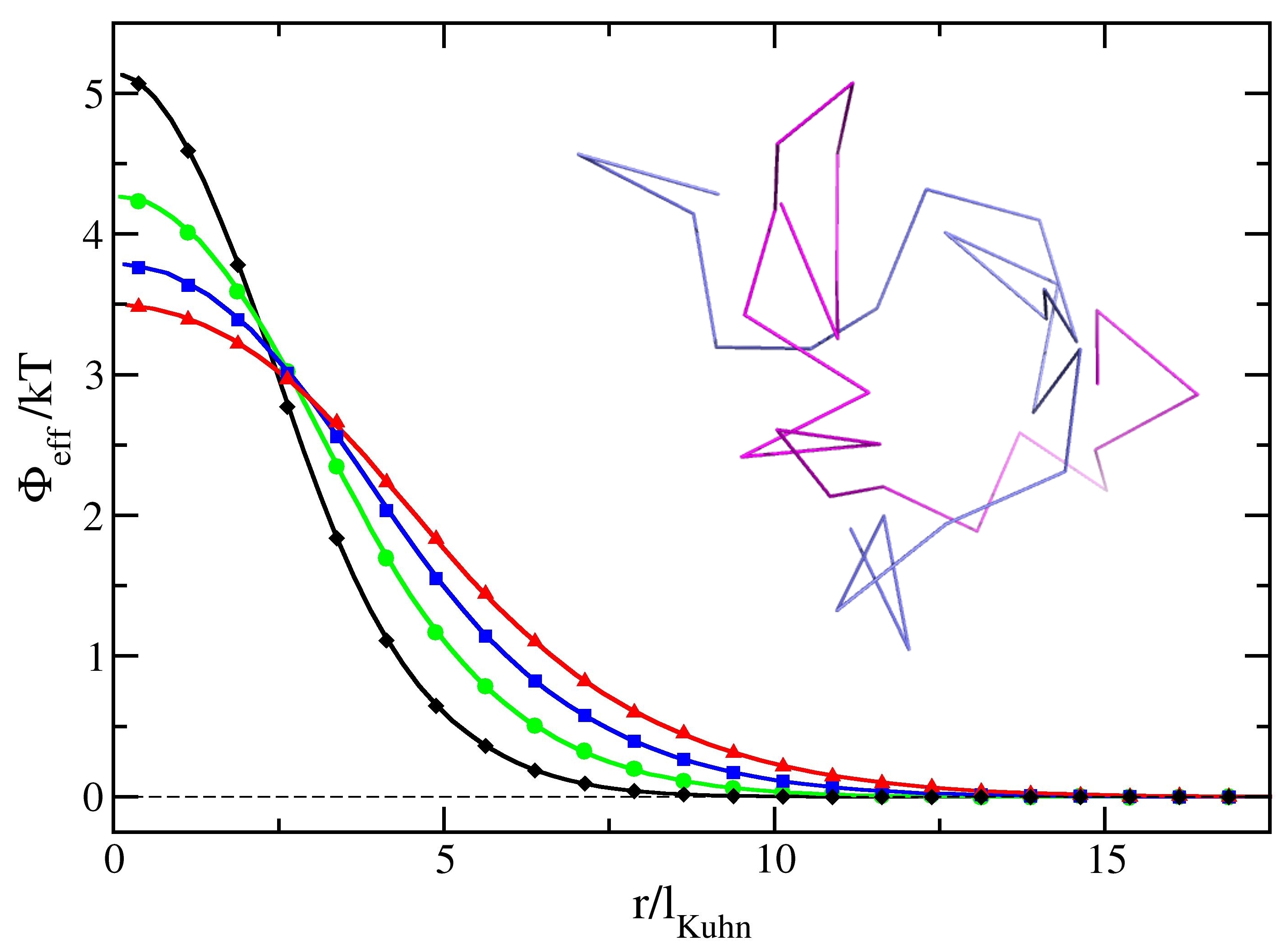
Fig.  1: (Color online) Comparison between Widom’s method (solid lines) and biased simulations (symbols) of the effective interaction $\Phi_{\rm eff}$ between two electrostatically charged polymer chains of length $20$ (diamonds), $30$ (circles), $40$ (squares) and $50l_{\rm Kuhn}$ (red, triangles) as a function of the distance between their centers of mass. The inset shows a simulation snapshot of two chains of $20l_{\rm Kuhn}$.

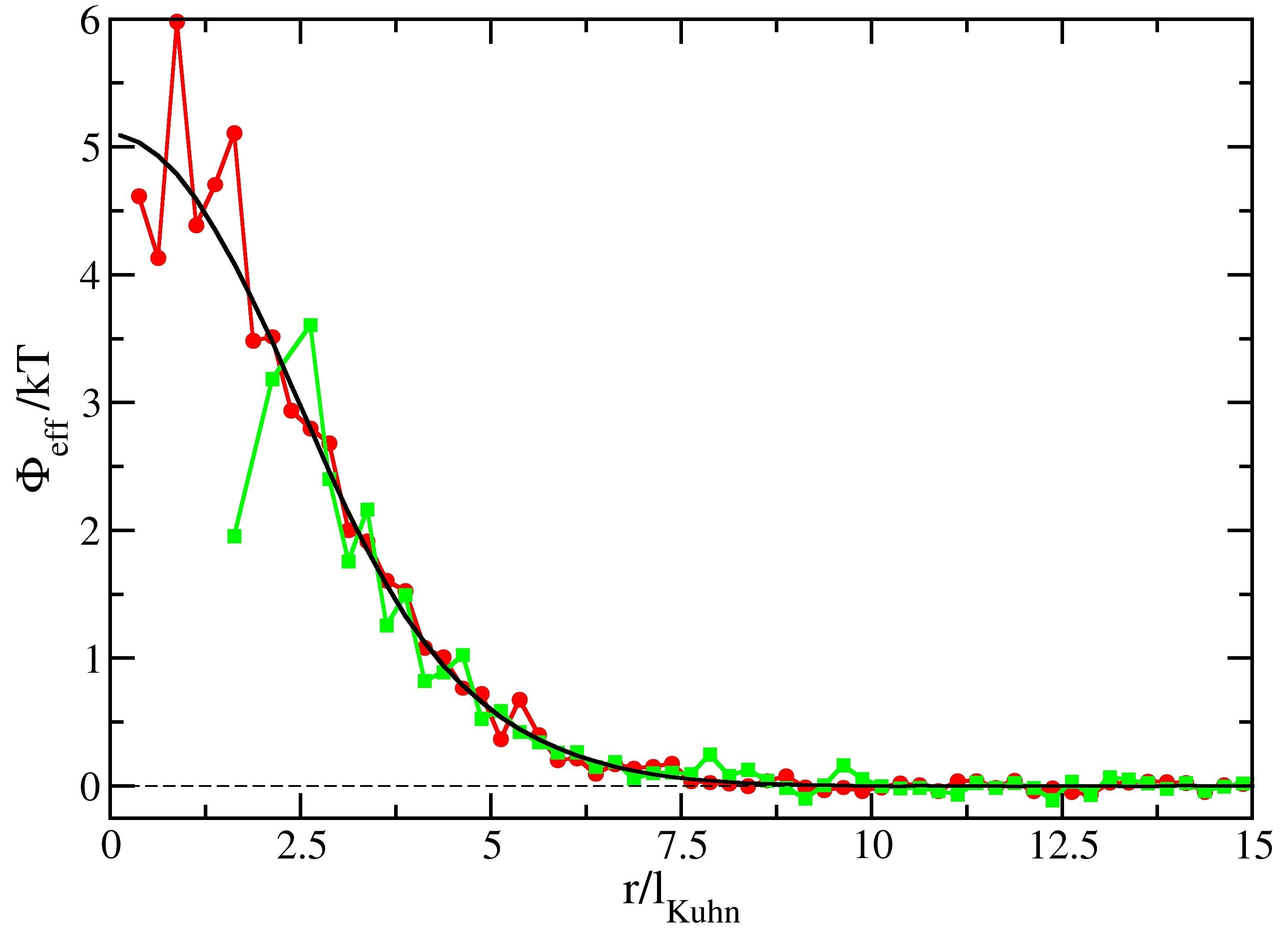
Fig.  2: (Color online) Comparison between Widom’s method (solid line), biased simulations (solid line with circles) and brute force calculations (solid line with squares) of the effective interaction $\Phi_{\rm eff}$ between two electrostatically charged polymers of length 20 after one hour of simulation time. While the data from Widom’s insertion is equilibrated, statistics on the data of the other two methods is still insufficient.

5.2 Colloids coated with electrostatic polymers

As a second example, we study a system of colloids coated with electrostatically charged polymers that can move on the colloid’s surface. In this case, we determine the effective interaction between the centers of the colloids rather than the centers of mass. The vertices of the chains interact amongst each other as described in Sec. 5.1, while the colloids are impenetrable spheres of fixed radius $R_{\rm coll}$. Again, we implement crankshaft and pivot moves for the polymer chains, but we also regrow them completely via a configurational bias MC algorithm¹², using 5 trial directions in each step of the regrowth. The colloids are subject to rotations and translations. Our model system is made of colloids of $R_{\rm coll}=4l_{\rm Kuhn}$, each coated with 10 chains of 5 Kuhn segments. For Widom’s method, we simulated $4\times 10^{6}$ cycles consisting of 250 MC steps to decorrelate the coating of the colloids before sampling 500 different distances between the colloids.

In Fig. 3 we see that the Widom particle insertion data perfectly reproduces the results of unbiased, brute force simulations, which we ran for $1\times 10^{7}$ MC sweeps. In the latter, each sweep consisted of $220$ MC moves (i.e. pivot or crankshaft move, configurational bias MC regrowth, colloid rotation or translation). While the brute force simulations needed two days of simulation time and were averaged over 6 different simulation runs to obtain reliable statistics, the data from a single simulation applying Widom’s method already shows decent statistics after as little as $5\times 10^{4}$ cycles, which corresponds to 1.5 hours of simulation time on a single processor of our cluster.

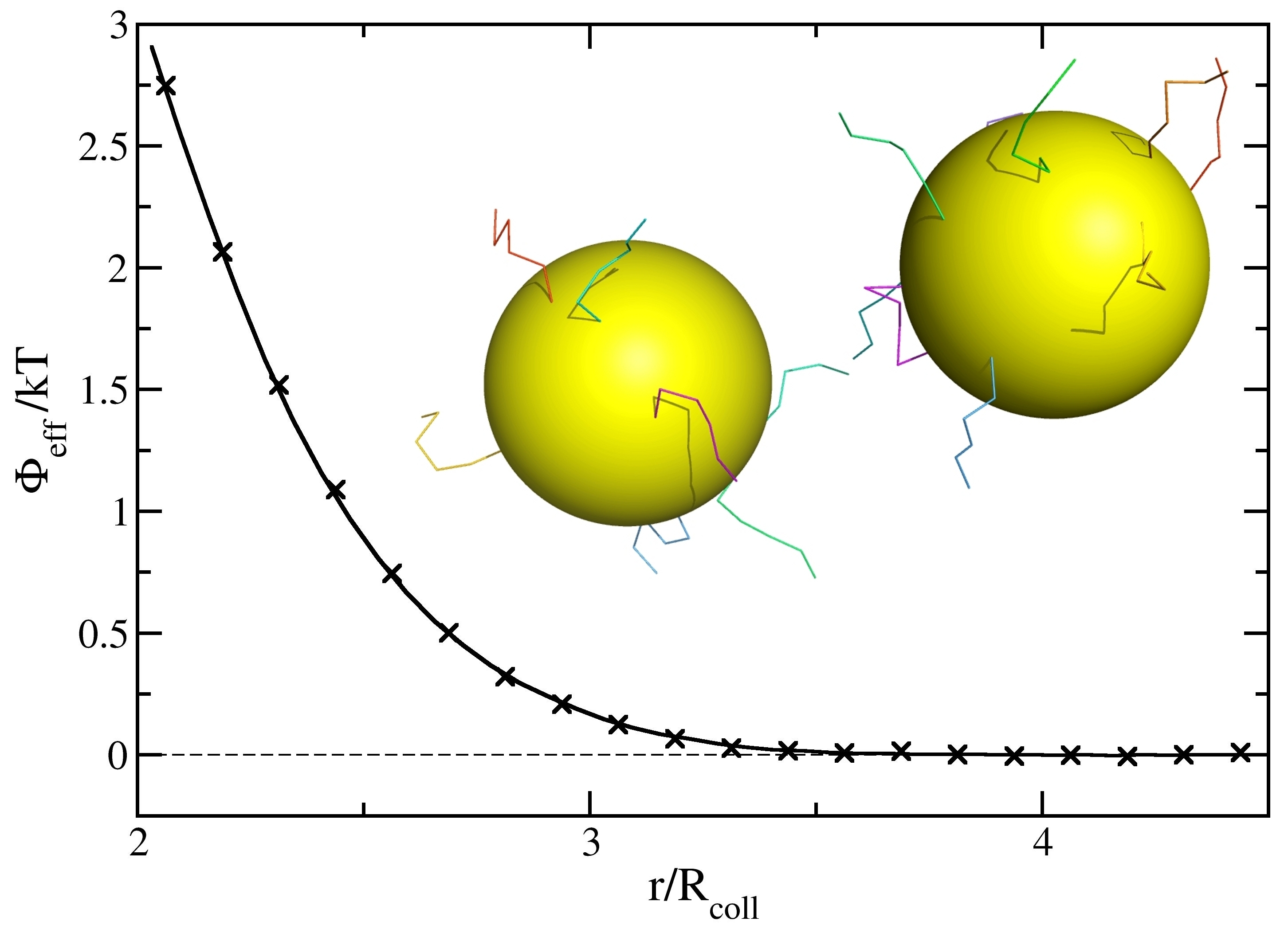
Fig.  3: (Color online) Comparison between Widom’s method (solid line) and brute force simulations (crosses) of the effective interaction $\Phi_{\rm eff}$ between two colloids of radius $R_{\rm coll}=4l_{\rm Kuhn}$ coated with 10 electrostatically charged polymer chains of length $5l_{\rm Kuhn}$ as a function of the distance between their centers. The inset shows a simulation snapshot of the colloids.

5.3 Amphiphilic dendrimers

Our final example concerns the determination of the effective interaction between two amphiphilic dendrimers^{6, 24}, which are expected to show clustering behavior at sufficiently high densities^{6, 25, 26, 27}.

We sample two different second-generation amphiphilic dendrimers. They have two central monomers and while the end-groups form a solvophilic shell, all inner monomers represent the solvophobic core. The bonds between monomers are modeled by the finitely extensible nonlinear elastic potential, while all other interactions between monomers are modeled by the Morse potential^{28, 29, 6}. For the parameters of the different interactions, we choose the same as for dendrimer $D_{5}$ and $D_{7}$ from Ref.30 and we refer to this reference for details.

Again, we implement Widom’s insertion method and compare our results to the effective interactions found in Ref.30 via umbrella sampling. For the umbrella sampling, 15 slightly overlapping windows with $R_{\rm max}=5R_{g}$ were used, where $R_{g}$ is the radius of gyration of a single dendrimer. The systems were then sampled for $2\times 10^{8}$ MC sweeps in each window. These simulations can be carried out in parallel. For Widom’s method, we sampled the dendrimers for $4\times 10^{6}$ MC cycles. In each of these cycles, each dendrimer was decorrelated in 280 single monomer displacements and the resulting configurations were used to sample 1000 different distances between them.

As can be seen from Fig. 4, Widom’s method manages to capture the interaction potential even at close approach of the dendrimers where deformations to the dendrimer’s conformations are expected. While Widom’s technique already gives reliable statistics for the effective interaction after as little as $5\times 10^{5}$ cycles, corresponding to 3h of simulation time, umbrella sampling had to be carried out on 15 processors for roughly a day to collect the necessary statistics.

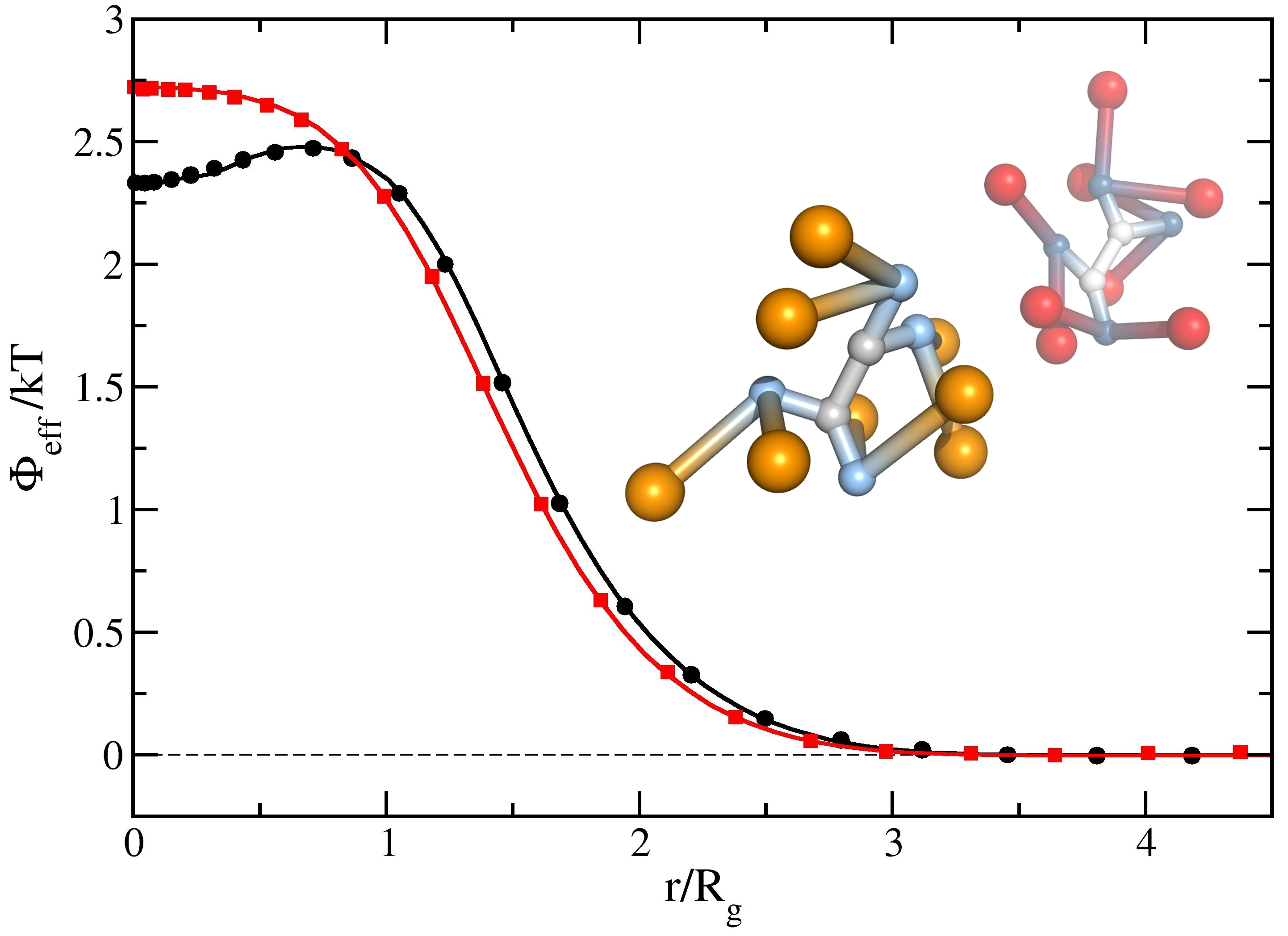
Fig.  4: (Color online) Comparison between Widom’s method (solid lines) and brute force simulations (symbols) of the effective interaction $\Phi_{\rm eff}$ between two amphiphilic $D_{5}$ (circles) and $D_{7}$ (squares) dendrimers as a function of the distance between their centers of mass. The inset shows a simulation snapshot of two dendrimers.

6 Conclusions

In this contribution we have shown that Widom’s particle insertion method can be adapted to determine the effective interaction between two mesoscopic particles in a completely unbiased, efficient way. While we showed the success of the method for three rather different model systems, this method can not be applied in its present form to particle insertion in an explicit solvent. Further, we expect the method to fail for those systems where close approach between the two particles leads to a very strong deformation of the molecules’ conformations that will not be sampled adequately in the ideal-gas reference system that we use to generate independent conformations. The usual way to test for the reliability or the failing of Widom’s method is the so-called overlapping distribution method^{31, 12}, where two simulations are needed: one of a one-particle system, inserting a second one at frequent intervals; and one of a two-particle system, removing one at frequent intervals. Widom’s method will only give reliable answers when the probability distributions of finding certain energy differences $\Delta U$ upon insertion and removal, respectively, have sufficient overlap¹². However, in these cases Widom’s method will at least allow for an educated guess of a biasing potential that can be used with one of the standard techniques, and will thereby allow for a considerable speed-up of the conventional methods.

In summary, the application of Widom’s particle insertion method to the determination of effective interactions between two mesoscopic particles has several advantages over the standard techniques: first, it allows for unbiased simulations, while the standard techniques require a guess of appropriate biasing potentials to force the system into close approaches. These potentials have to be determined with high accuracy in an iterative process, or if less precise potentials are used, simulations in multiple windows of different separation ranges are required. Furthermore, Widom’s method is very easy to implement. Finally, biased or brute force simulations rely on the diffusion of the particles through the simulation box, where each change in separation will only be accepted with a certain probability depending on the ratio between the Boltzmann weights of the old and the new configurations. This makes the relative diffusion of highly entangled particles slow and can lead to slow statistical fluctuations in the data of the effective interaction. By contrast, within Widom’s method particles are simply placed at a given separation and the intermolecular energy difference is measured, without having to employ any acceptance/rejection step. Therefore, Widom’s particle insertion method immediately allows for an exploration of even the closest approach and will give reliable statistics for the effective interaction for all ranges of separation within very short simulation times. For the cases that we have studied, this makes Widom’s particle insertion method the better technique to compute effective interactions between mesoscopic particles.

7 Acknowledgements

We thank S. Abeln from the Vrije Universiteit Amsterdam and C. N. Likos from the University of Vienna for highly stimulating discussions. BMM acknowledges funding from the EU via FP7-PEOPLE-IEF-2008 No. 236663. DF acknowledges financial support from the Royal Society of London (Wolfson Merit Award) and from the ERC (Advanced Grant agreement 227758).

References

- Likos 2001 C. N. Likos, Phys. Rep., 2001, 348, 267.
- Bolhuis et al. 2001 P. G. Bolhuis, A. A. Louis, J.-P. Hansen and E. J. Meijer, J. Chem. Phys., 2001, 114, 4296–311.
- Jusufi et al. 2002 A. Jusufi, C. N. Likos and H. Löwen, Phys. Rev. Lett., 2002, 88, 018301.
- Denton 2003 A. R. Denton, Phys. Rev. E, 2003, 67, 11804.
- Götze et al. 2004 I. O. Götze, H. M. Harreis and C. N. Likos, J. Chem. Phys., 2004, 120, 7761.
- Mladek et al. 2008 B. M. Mladek, G. Kahl and C. N. Likos, Phys. Rev. Lett., 2008, 100, 028301.
- Capone et al. 2010 B. Capone, J.-P. Hansen and I. Coluzza, Competing micellar and cylindrical phases in semi-dilute diblock copolymer solutions, doi:10.1039/C0SM00738B, 2010.
- Hansen and McDonald 2006 J.-P. Hansen and I. R. McDonald, Theory of Simple Liquids, Academic Press, London, 3rd edn, 2006.
- Krüger et al. 1989 B. Krüger, L. Schäfer and A. Baumgärtner, J. Phys. (France), 1989, 50, 3191.
- Wang and Landau 2001 F. Wang and D. P. Landau, Phys. Rev. Lett., 2001, 86, 2050–2053.
- Torrie and Valleau 1977 G. M. Torrie and J. P. Valleau, J. Comput. Phys., 1977, 23, 187–199.
- Frenkel and Smit 2002 D. Frenkel and B. Smit, Understanding Molecular Simulation, Academic Press, London, 2nd edn, 2002.
- Chandler 1987 D. Chandler, Introduction to Modern Statistical Mechanics, Oxford University Press, Oxford, 1987.
- Ferrenberg and Swendsen 1988 A. M. Ferrenberg and R. H. Swendsen, Phys. Rev. Lett., 1988, 61, 2635–2638.
- Kumar et al. 2004 S. Kumar, J. M. Rosenberg, D. Bouzida, R. H. Swendsen and P. A. Kollman, J. Comput. Phys., 2004, 13, 1011 – 1021.
- Widom 1978 B. Widom, J. Stat. Phys., 1978, 19, 563–574.
- Metropolis et al. 1953 N. Metropolis, A. W. Rosenbluth, M. N. Rosenbluth, A. H. Teller and E. Teller, J. Chem. Phys., 1953, 21, 1087.
- Zhang et al. 2001 Y. Zhang, H. Zhou and Z.-C. Ou-Yang, Biophys. J., 2001, 81, 1133.
- Smith et al. 1996 S. B. Smith, Y. Cui and C. Bustamante, Science, 1996, 271, 795.
- 20 B. M. Mladek and D. Frenkel, unpublished.
- Lal 1969 M. Lal, Molec. Phys., 1969, 17, 57.
- Madras and Sokal 1988 N. Madras and A. D. Sokal, J. Stat. Phys., 1988, 50, 109.
- Baumgärtner 1984 A. Baumgärtner, in Applications of the Monte Carlo method in statistical physics, ed. K. Binder, Springer, Berlin, 1984, ch. Simulations of polymer models.
- Lenz et al. 2009 D. A. Lenz, R. Blaak and C. N. Likos, Soft Matter, 2009, 5, 2905–2912.
- Mladek et al. 2006 B. M. Mladek, D. Gottwald, G. Kahl, M. Neumann and C. N. Likos, Phy, 2006, 96, 45701.
- Mladek et al. 2008 B. M. Mladek, P. Charbonneau, C. N. Likos, D. Frenkel and G. Kahl, J. Phys.: Condens. Matter, 2008, 20, 494245.
- 27 D. A. Lenz, B. M. Mladek, C. N. Likos, G. Kahl and R. Blaak, unpublished.
- Welch and Muthukumar 1998 P. Welch and M. Muthukumar, Macromolecules, 1998, 31, 5892–5897.
- Ballauff and Likos 2004 M. Ballauff and C. N. Likos, Angew. Chem. Int. Ed., 2004, 43, 2998–3020.
-
30
B. M. Mladek, PhD thesis, TU Vienna,
www.ub.tuwien.ac.at/
diss/AC05035480.pdf, 2008. - Shing and Gubbins 1982 K. S. Shing and K. E. Gubbins, Mol. Phys., 1982, 46, 1109.