Importance of far-infrared mapping in a spiral galaxy: AKARI observation of M 81

Abstract

The importance of the far-infrared (FIR) mapping is demonstrated for a face-on spiral galaxy, M 81, by analyzing its imaging data at 65, 90, and 140 $\micron$ taken by AKARI. Basic products are the dust temperature map, the dust optical depth map, and the colour–colour diagram. The main features are as follows. (i) The dust temperature derived from the total fluxes at 90 $\micron$ and 140 $\micron$ reflects the relatively low temperatures seen in the interarm and spiral arms excluding the warm spots, rather than the high temperatures in warm spots and the centre. This indicates that the total FIR luminosity is dominated by the dust heated by the general interstellar radiation field. (ii) The galaxy is more extended at 140 $\micron$ than at the other shorter wavelengths, which reflects the radial dust temperature gradient. (iii) The dust optical depth derived from the FIR mapping is broadly consistent with that estimated from the FIR-to-ultraviolet luminosity ratio. (iv) The FIR colour–colour diagram is useful to identify a ‘contamination’ of warm dust. The existence of small-scale warm star-forming regions is supported in the bright spots along the spiral arms. This contamination also leads to an underestimate of dust optical depth (or dust column density).

1 Introduction

The far-infrared (FIR) emission from galaxies is dominated by the thermal emission from dust grains (e.g. Harper & Low, 1973), and is known to be a good indicator of star formation rate (e.g. Kennicutt, 1998; Inoue, Hirashita, & Kamaya, 2000). Since the major heating source of dust grains is usually stellar radiation, the FIR colour, which reflects the dust temperature, is one of the most direct indicators of the interstellar radiation field (ISRF). Moreover, the FIR emission is usually optically thin in the ISM, which means that we can trace all the radiation over the entire column.

Spatially resolved images of galaxies are required to study the dust properties in different regions of a galaxy and the characteristics of individual star-forming regions. Also, since only integrated global properties are observable for distant star-forming galaxies, it is important to clarify the relation between the global and local characteristics. Specifically we should distinguish whether the major dust heating comes from individual star-forming regions or general ISRF (e.g. Walterbos & Greenawalt, 1996) to clarify the major origin of the dust heating source responsible for the FIR emission. However, because the spatial resolution of FIR observation is generally poor, only galaxies with large angular size can be well resolved.

M 81 is particularly suitable for our purpose because (i) it is a nearby big galaxy with a face-on geometry; (ii) it can be compared with another well-known spiral galaxy, the Milky Way; and (iii) it is within a field of view of the scan observation of AKARI, which is useful to quantify the global properties and to subtract the background.

Which wavelengths in FIR are necessary? At long wavelengths ($\ga 90~{}\micron$), the dust emission is mainly contributed by relatively large grains in radiative equilibrium with the stellar radiation field. However, an emission excess in shorter wavelengths ($\la$ 65$\micron$) is usually observed, which comes from very small dust grains suffering from stochastic heating, that is, heated transiently to a high temperature (Aannestad & Kenyon, 1979; Draine & Anderson, 1985). In order to estimate the large grain temperature, which can be used to indicate the intensity of the ambient stellar radiation, at least two bands are needed at wavelengths $\ga 90~{}\micron$. Furthermore, we require three wavelengths in the FIR to make a FIR colour–colour diagram. It has been shown that the FIR colour–colour relation of galaxies is useful to derive the wavelength dependence of dust emissivity (Dale et al., 2001; Nagata et al., 2002; Hibi et al., 2006). The FIR colour–colour relations in the Galactic disc and the Large/Small Magellanic Clouds are tight, indicating that the wavelength dependence of dust FIR emission can be considered to be uniform within and among those galaxies (Shibai, Okumura, & Onaka, 1999; Hibi et al., 2006). Such a common wavelength dependence of dust emission can be nicely reproduced by a common grain optical properties and size distribution (Hirashita, Hibi, & Shibai, 2007). In this paper, the FIR colour-colour diagram also proves to be important for investigating the dust emission characteristics.

Slow-scan data of Far Infrared Surveyor (FIS) onboard AKARI (Murakami et al., 2007; Kawada et al., 2007) with the 65, 90, and 140 $\micron$ bands is enough for the above requirements. (We do not use the 160 $\micron$ data because the data quality is not good enough for our purpose.) The 90 and 140 $\micron$ bands are used to estimate the large grain equilibrium temperature, and a colour–colour diagram can be made with the 65, 90, and 140 $\micron$ bands. Besides, by using the AKARI FIS data, a direct comparison among M 81 and a large number of galaxies in the AKARI All-Sky data (Yamamura et al., 2009) can be made because of the common observational facility. Very recently, Suzuki et al. (2010) has reported an analysis of the AKARI data of M 81. They focus on the star formation law but do not investigate the details of the dust temperature distribution within the galaxy and the FIR colour–colour diagram. M 81 is also observed by the Spitzer Space Telescope (Pérez-González et al., 2006), whose 70 $\micron$ and 160 $\micron$ data can be compared with our data. However, the dust temperature from the 70 $\micron$ and 160 $\micron$ bands can overestimate the equilibrium temperature because of the possible contamination in the 70 $\micron$ emission by the stochastically heated very small grains. Thus, another FIR band at $\ga 90~{}\micron$ is desirable. This galaxy has recently been observed by Bendo et al. (2010) with Herschel Space Observatory (Pilbratt et al., 2010), whose long-wavelength coverage is particularly useful to examine the robustness of our analysis against the inclusion of long-wavelength data. Although the Herschel data are better than our AKARI data both in the spatial resolution and sensitivity, we concentrate on the AKARI data in this paper because not only the data of M 81 is available but also the All-Sky Survey data can be used to test if the FIR colours obtained for M 81 can be discussed in terms of a large number of other nearby galaxies taken by the same facility.

In this paper, we aim to point out the importance of FIR mapping data by deriving some fundamental quantities about dust (dust temperature, dust optical depth, etc.). At the same time, we try to clarify the relation between global (integrated) quantities and spatially resolved quantities. Some important features in the FIR colour–colour diagram of a spatially resolved image is also focused on. The method used in this paper is general and can be applied to future data taken by Herschel or the Atacama Large Millimetre/submillimetre Array (ALMA).

This paper is organized as follows. We explain the data analysis in Section 2, and describe some basic results related to global properties such as morphology and radial dependence in Section 3. We investigate the distribution of dust temperatures and the colour–colour diagram in Section 4. We discuss the results obtained for M 81 in general contexts in Section 5. Finally, Section 6 gives the conclusion. The distance to M 81 is assumed to be 3.63 Mpc (Freedman et al., 1994) throughout this paper. At this distance, 1 arcmin corresponds to 1.06 kpc.

2 Data analysis

M 81 was observed by AKARI/FIS as a pointed observation (PI: FIS Team). The data are taken from Data Archives and Transmission System. Photometric observations were performed with four bands: N60 (central wavelength: 65 $\micron$), WIDE-S (90 $\micron$), WIDE-L (140 $\micron$), and N160 (160 $\micron$) with an observational mode of FIS01 (photometry/mapping mode), a reset interval of 0.5 s and a scan speed of 15 arcsec s^-1. We utilize the images of the 65 $\micron$, 90 $\micron$, and 140 $\micron$ bands. The quality of the 160 $\micron$ band image is not good enough for our purpose. The FIS observation of M 81 is composed of two pointings: one covers almost all the M 81 area except for the south-east edge, which is observed by the second observation. We combine those two images to obtain the entire M 81 image after the background subtraction (Section 2.3), and the analysis procedures before combining the images are identical for the two images. The measured FWHMs of point spread function are $37^{\prime\prime}$, $39^{\prime\prime}$, and $58^{\prime\prime}$ (Kawada et al., 2007), which correspond to 650 pc, 690 pc, and 1000 pc, respectively, at M 81. Thus, internal structures such as spiral arms can be clearly identified on the images (Section 3.1).

2.1 FIS Slow-Scan Tool

The raw data were reduced by using the FIS Slow-Scan Tool (version 20070914; Verdugo, Yamamura, & Pearson 2007). The process includes flagging of bad data, measurement of sky signal, dark and response correction, flat-fielding, and construction of co-added images. We used the local-flat for the flat-fielding. The output image grid size is chosen to be 30”, which is about half of the beam size of 140  $\micron$. We confirmed that the following results are not sensitive to the selection of the grid size. The final image is smoothed with a length of $\sim 40^{\prime\prime}$ for the SW (65 $\micron$ and 90 $\micron$) images and $\sim 60^{\prime\prime}$ for the LW (140 $\micron$) image to avoid the effect of small scale detector noise.

It is known that the AKARI/FIS detectors underestimate the total flux probably because of the slow response (Shirahata et al., 2008). Thus, we multiply the correction factors for the intensity, 1.7 for 65 $\micron$ and 90 $\micron$, and 1.9 for 140 $\micron$, are multiplied to each band. Because the factors are similar to all the bands, the colours (flux ratios) and dust temperatures are not significantly affected by this correction.

2.2 Colour correction

Since the intensity at the central wavelength is derived by assuming a flat spectrum ($\nu I_{\nu}=\mbox{constant}$) in the FIS Slow-Scan Tool, a colour correction should be applied. We applied correction to the WIDE-S (90 $\micron$) and WIDE-L (140 $\micron$) fluxes, assuming a spectral shape of $I_{\nu}\propto\nu^{\beta}B_{\nu}(T_{\mathrm{d}})$, where $T_{\mathrm{d}}$ is the dust temperature, $\beta$ is the emissivity index, and $B_{\nu}(T)$ is the Planck function. The emissivity index $\beta$ is chosen to be 2 in this paper unless otherwise stated. The value of $\beta$ is dependent on the grain composition, and $\beta=2$ is appropriate for astronomical silicate and graphite in Draine & Lee (1984). We apply $T_{\mathrm{d}}=27$ K and 19 K for WIDE-S and WIDE-L, respectively; the former (latter) temperature is derived from the total fluxes of M 81 at N60 and WIDE-S (WIDE-S and WIDE-L) (see Section 3.2). Consequently, the correction factor is 0.92 and 0.94 for the WIDE-S and WIDE-L fluxes, respectively, and the flux obtained by the Slow Scan Tool is divided by these factors. The uncertainty caused by the colour correction (5 per cent for WIDE-S and 1 per cent for WIDE-L for the temperature range observed in the M 81 disc; Section 4.1) is smaller than the errors caused by the background fluctuation. For the narrow band N60 (65 $\micron$) we do not apply the correction, since the colour correction only changes the flux by less than 3 per cent.

2.3 Background subtraction

Bright stripes along the scan direction caused by glitches or non-uniform detector sensitivity are observed in all the three bands. In order to eliminate these structures, the background levels are estimated for each line along the scan direction by averaging the intensities in the two sections before and after the scan of the M 81 main body with a separation of about $18^{\prime}$ and a total length of about $20^{\prime}$, and then subtracted. The RMSs of the background are 1.3, 0.7, 2.9 MJy sr^-1 for the 65, 90, and 140 $\micron$ bands, respectively. These values are estimated before eliminating the stripes to show the original uncertainty including the non-uniform sensitivity and the time variability of the detector response.

2.4 Matching the positions

We matched the positions of the images taken by two detectors, SW (N60 and WIDE-S) and LW (WIDE-L) according to the position of central peak of the galaxy image. The uncertainty in the relative position between the detectors is well below the grid size.

2.5 The physical quantities derived from the data

The intensity (surface brightness) at a wavelength $\lambda$ (frequency $\nu\equiv c/\lambda$, where $c$ is the light speed) in each grid is denoted as $I_{\nu}(\lambda)$. The intensity ratio, $I_{\nu}(\lambda_{1})/I_{\nu}(\lambda_{2})$, is called $\lambda_{1}-\lambda_{2}$ colour in this paper. We derive the dust temperature $T_{\mathrm{d}}$ in each grid as follows. Since the dust emission is optically thin in the FIR (Section 4.1), $I_{\nu}(\lambda)=\tau(\lambda)B_{\nu}(T_{\mathrm{d}})$, where $\tau(\lambda)$ is the optical depth at wavelength $\lambda$. The functional form of the optical depth is assumed to be $\tau(\lambda)=A\nu^{2}$ ($\nu=c/\lambda$) with an unknown constant $A$, which is independent of the frequency. This functional form for the optical depth indicates that the frequency dependence of the dust emission coefficient follows $\propto\nu^{\beta}$ with $\beta=2$. Then, with two wavelengths ($\lambda_{1}$ and $\lambda_{2}$) selected, a set of equations, $I_{\nu}(\lambda_{1})=\tau(\lambda_{1})B_{\nu}(T_{\mathrm{d}})|_{\lambda_{1}}$ and $I_{\nu}(\lambda_{2})=\tau(\lambda_{2})B_{\nu}(T_{\mathrm{d}})|_{\lambda_{2}}$, is solved to obtain $T_{\mathrm{d}}$ and $A$. The dust temperature $T_{\mathrm{d}}$ determined from wavelengths of 90 $\micron$ and 140 $\micron$ represents the temperature of large grains in radiative equilibrium with the ambient radiation field (e.g. Li & Draine, 2001), and it is denoted as $T_{\mathrm{LG}}$.

It is convenient to convert $\tau(\lambda)=A\nu^{2}$ to a commonly used indicator of dust optical depth. We choose $A_{V}$ (the extinction in $V$ band in units of magnitude) for such an indicator. We adopt the Galactic extinction curve for the conversion from $\tau(\lambda)$ to $A_{V}$ as derived by Weingartner & Draine (2001) for $R_{V}=3.1$: $A_{V}=\mathcal{C}(\lambda)\tau(\lambda)$, where the factor $\mathcal{C}(\lambda)$ is $8.3\times 10^{2}$ for 90 $\micron$ and $1.9\times 10^{3}$ for 140 $\micron$. Although we derive $A_{V}$ by using the 90 $\micron$ values, we obtain the same value for $A_{V}$ also from the 140 $\micron$ values because $\mathcal{C}(\lambda)\propto\lambda^{2}$ holds within 10 per cent between 90 and 140 $\micron$.

3 Global Properties

Figure 1: Images of M 81. (a) The 90 $\micron$ image. The circles define various regions used for the analysis of the colour–colour relation in Section 4.2: the central region (C), the spiral arm regions (S1, S2, and S3), and the interarm regions (I1, and I2). (b) The H$\alpha$ image taken by Cheng et al. (1997) (grey scale) overlaid with the 90 $\micron$ brightness contours. The highest contour shows 0.71 times the peak intensity and the intensity ratio of two adjacent contours is set to be 0.71.

3.1 Morphological features

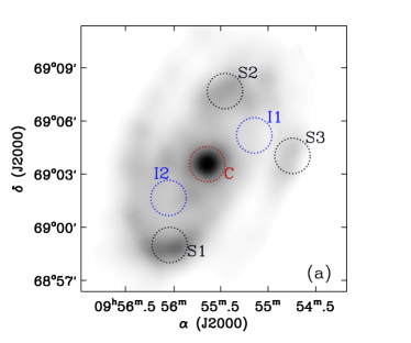
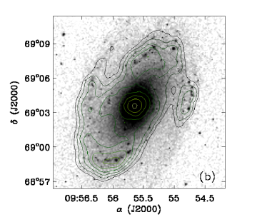
In Fig. 1, we show the 90 $\micron$ image. The central bright peak, the spiral structures, and the spots along the spiral arms are clear. In order to examine the correspondence between the FIR brightness and the star formation activity in M 81, we compare our FIR image with the H$\alpha$ image taken from the NASA/IPAC Extragalactic Database (NED) (originally from Cheng et al. 1997). The FIR emission really traces the H$\alpha$ central peak, the H$\alpha$ spiral arms, the H ii regions along the spiral arms. This confirms that the FIR emission is a good tracer of the star formation activities in galaxies.

3.2 Spectral Energy Distribution

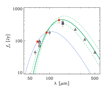
The measured total fluxes, $f_{\nu}$, at 65, 90, and 140 $\micron$ are shown in Fig. 2 and Table 1 together with the data taken from the literature. The fluxes are estimated by integrating intensities over a rectangular region of width $15^{\prime}$ and length $18^{\prime}$ covering the galaxy main body. We conservatively adopt flux errors of 10 per cent for the 65 $\micron$ band and the 90 $\micron$ band and 20 per cent for the 140 $\micron$ band (Hirashita et al., 2008). As shown in Table 1, we obtain the fluxes consistent with Suzuki et al. (2010) within the errors.

Figure 2: FIR SED of M 81. The filled squares show our measurements, while the others are taken from the literature: The open diamonds at 60 $\micron$ and 100 $\micron$ are taken from the IRAS data (Rice et al., 1988), the open squares at 70 $\micron$ and 160 $\micron$ from the Spitzer data (Pérez-González et al., 2006; Dale et al., 2007), and the open triangles from the Herschel data (Bendo et al., 2010). The solid (dotted) line shows the single-temperature SED which explains our measurements at 90 $\micron$ and 140 $\micron$ (65 $\micron$ and 90 $\micron$). The dashed lines show the SEDs at the temperature of upper and lower bound of $T_{\mathrm{LG}}$ estimated by using the upper and lower fluxes at 90 $\micron$ and 140 $\micron$.

Table 1: Observational fluxes in units of Jy for the entire M 81 (global) and the individual regions shown in Fig. 1.

Wavelength	65 $\micron$	90 $\micron$	140 $\micron$
Global	94 $\pm$ 9	177 $\pm$ 18	419 $\pm$ 84
Global (S10) a	$70\pm 20$	$189\pm 40$	$356\pm 140$
C	9.21	12.8	16.3
S1	3.61	6.05	10.7
S2	3.42	6.52	13.0
S3	1.65	2.71	5.32
I1	2.06	4.80	10.8
I2	2.12	5.07	11.7

^a Measurements by Suzuki et al. (2010).

Note. The conservative errors are 10 per cent for 65 and 90 $\micron$, and 20 per cent for 140 $\micron$.

We also show two spectral energy distributions (SEDs) which fit the data at 90 and 140 $\micron$ and those at 65 and 90 $\micron$ with the functional form given in Section 2.5 (i.e. $f_{\nu}\propto\nu^{2}B_{\nu}(T_{\mathrm{d}})$). We observe that the SED which fits the 90 $\micron$ and 140 $\micron$ fluxes underproduces the 65 $\micron$ flux. This indicates the contribution of very small grains (VSGs) to the emission at $\la 65\,\micron$ (Aannestad & Kenyon, 1979; Draine & Anderson, 1985): Small grains with radii $\la 10$ nm are stochastically (i.e. not in radiative equilibrium) heated to a high temperature, contributing to the intensity at the short ($\la 65\,\micron$) wavelengths. The dust temperature $T_{\mathrm{d}}$ derived from the 90 $\micron$ and 140 $\micron$ fluxes is 18.6 K, while that derived from the 65 $\micron$ and 90 $\micron$ is 27.3 K. The former temperature is interpreted to be the one of large grains which are in radiative equilibrium with the ambient ISRF ($T_{\mathrm{LG}}$), while the latter does not present any physical dust temperature because of the contamination of stochastically heated very small grains to the 65 $\micron$ flux. To estimate the uncertainty in $T_{\mathrm{LG}}$, we use the upper (lower) and lower (upper) values for the 90 and 140 $\micron$ fluxes and obtain the upper (lower) temperature as shown in Fig. 2: 20.5 and 17.0 K for the upper and lower temperatures, respectively. Thus, we finally obtain an estimate for the large grain temperature as $T_{\mathrm{LG}}=18.6^{+1.9}_{-1.6}$ K from the global SED. We observe that the Spitzer and Herschel data at $\lambda\geq 160~{}\micron$ are broadly consistent with our SED fit to the 90 $\micron$ and 140 $\micron$ data within the errors.

Pérez-González et al. (2006) have shown that the Spitzer data can be fitted with two dust temperatures: their colder component with a temperature of $18\pm 2$ K has a consistent temperature with our $T_{\mathrm{LG}}$, while their warmer component with $53\pm 7$ K shows a much higher temperature because they also used the 24 $\micron$ data. The temperature estimated by the Herschel data is $17.8\pm 0.6$ K (Bendo et al., 2010). Our estimate of the large grain temperature is consistent with the Spitzer and Herschel results within the errors.

As a global quantity, we derive the total infrared (TIR) luminosity (the integrated luminosity between 8 and 1000 $\micron$), which is used later in Section 4.1. For this aim, we first estimate the total flux traced by AKARI FIS. The AKARI FIR flux, $f_{\mathit{AKARI}}$ is defined by Hirashita et al. (2008) to estimate the total flux in the wavelength range of 50–170 $\micron$:

$$f_{\mathit{AKARI}} \equiv f_{\nu}(65~{}\micron)\Delta\nu(\mbox{{N}60})+f_{\nu}(90~{}\micron)\Delta\nu(\mbox{{WIDE-S}})$$ (1)

$$+f_{\nu}(140~{}\micron)\Delta\nu(\mbox{{WIDE-L}}),$$

where $f_{\nu}(\lambda)$ is the flux per unit frequency at wavelength $\lambda$, and $\Delta\nu(\mbox{band})$ denotes the frequency width covered by the band. According to Kawada et al. (2007), we adopt $\Delta\nu(\mbox{N60})=1.58$ THz, $\Delta\nu(\mbox{{WIDE-S}})=1.47$ THz, and $\Delta\nu(\mbox{{WIDE-L}})=0.831$ THz. With $f_{\mathit{AKARI}}$, the AKARI FIR luminosity, $L_{\mathit{AKARI}}$, is estimated as

$$L_{\mathit{AKARI}}=4\pi D^{2}f_{\mathit{AKARI}},$$ (2)

where $D=3.63$ Mpc is the distance to M 81. We obtain $L_{\mathit{AKARI}}=(3.1\pm 0.6)\times 10^{9}~{}\mathrm{L}_{\sun}$. Considering that the 10–20 per cent errors in the flux, we put an error of 20 per cent also to the luminosity.

Next, we relate the AKARI luminosity and the TIR luminosity. There is a good correlation between $L_{\mathit{AKARI}}$ and $L_{\mathrm{TIR}}$ (total infrared luminosity emitted by dust) in the AKARI FIS Bright Source Catalogue, the first primary catalogue from the AKARI All-Sky Survey (Yamamura et al., 2009), as shown by Takeuchi et al. (2010):

$$\log L_{\mathrm{TIR}}=0.940\log L_{\mathit{AKARI}}+0.914.$$ (3)

With this empirical formula, $L_{\mathrm{TIR}}=(6.9\pm 1.4)\times 10^{9}~{}\mathrm{L}_{\sun}$ for M 81. This luminosity is divided by $4\pi D^{2}$ to obtain the total infrared flux, $F_{\mathrm{TIR}}=1.7\times 10^{-8}$ erg cm^-2 s^-1. Considering that the flux may be uncertain by 20 per cent, it would be appropriate to put a 20 per cent error for each flux or luminosity. Suzuki et al. (2010) obtained smaller luminosity $(4.0\pm 0.2)\times 10^{9}$ L_☉ for the total FIR luminosity. They consider contributions from two components: a cold component with a temperature of 22 K and a warm component with a temperature of 64 K, but these two components do not include the contribution from the emission at $<20~{}\micron$.

We can also check the consistency of the dust mass with the Herschel data. The total dust mass, $M_{\mathrm{d}}$, is estimated as

$$M_{\mathrm{d}}=\frac{f_{\nu}(\lambda)D^{2}}{\kappa_{\nu}B_{\nu}(T_{\mathrm{d}})},$$ (4)

where $\kappa_{\nu}$ is the mass absorption coefficient at a frequency $\nu$. Using the measured flux at 90 $\micron$, the dust temperature derived from the 90 and 140 $\micron$ data, and $\kappa_{\nu}=34$ cm² g^-1 at 90 $\micron$ (Weingartner & Draine, 2001), we obtain $M_{\mathrm{d}}=(3.2\pm 0.6)\times 10^{7}~{}\mathrm{M}_{\sun}$, where an error of 20 per cent is applied because of the flux uncertainty. This value is consistent with the dust mass ($3.4\times 10^{7}~{}\mathrm{M}_{\sun}$) obtained by the Herschel observation (Bendo et al., 2010).

3.3 Radial dependence

In Fig. 3, we show the radial profiles in the three bands. The radial distances ($r$) are deprojected by considering the position angle (157 degree) and the inclination angle (57 degree) taken from NED. The inclination angles given in NED range from 55 to 63 degree. Therefore the deprojected radius is uncertain by 10 per cent. The radius from the centre is divided into bins with a width of 50 arcsec, and the intensities of the pixels contained in each radius bin is averaged to obtain the intensity as a function of radius. The standard deviation for each radius bin is also shown with the bar. The flux errors are much smaller than the standard deviations.

Figure 3: Intensity profiles in various wavelengths. The diamonds, triangles, and squares represent the averaged intensities as a function of deprojected radial distance in the 65, 90, and 140 $\micron$ bands, respectively. The bars on the individual data points represent the standard deviation, not the errors. The solid lines are the fitting results with linear slopes for $r>150$ arcsec.

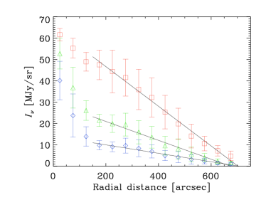
The radial profile can be divided into two components: bulge ($r<150$ arcsec) and disc ($r\geq 150$ arcsec). The 65 and 90 $\micron$ band images show a bright bulge where the intensity increases rapidly as the radius decreases, while the 140 $\micron$ image does not have such a sharp rise. The difference in the ‘sharpness’ of the bulge component among different bands is due to the high dust temperatures, which reflect an intense radiation from the active galactic nucleus (AGN) or from the stars with high surface density. The bulge component is not prominent also in the long-wavelength Herschel SPIRE data (Sauvage et al., 2010).

For the disk part, all the intensities in the three bands show a linear slope along the radius. The linear slope means that the dust emission is radially more extended than the stellar emission, whose radial profile drops exponentially (e.g. Baggett, Baggett, & Anderson, 1998). Although Sauvage et al. (2010) apply a fitting with exponential or Gaussian function to the FIR radial profile of the Herschel data, the fit is not necessarily good. The dispersion shown by the bars is relatively large around $r\sim 400$ arcsec. This radius corresponds to the radial extent of the spiral arms.

To compare the radial extents in the three bands, we show the radial profiles of the colours, $I_{\nu}(140~{}\micron)/I_{\nu}(90~{}\micron)$ and $I_{\nu}(65~{}\micron)/I_{\nu}(90~{}\micron)$ in Fig. 4. The former rises as the radius increases, showing that the 140  $\micron$ image is more extended than 90  $\micron$, while the latter dose not show such a clear trend. The slight enhancement of the $65\,\micron-140\,\micron$ colour and the plateau of the $140\,\micron-90\,\micron$ colour around $r=6$ arcsec are caused by the relatively high temperature in the spiral arms.

Because of the linear-slope behaviour of the radial profile, the radial extent is well defined by the intercepts on the $x$ axis in Fig. 3. The radial extents defined in this way are 706, 674, and 702 arcsec for the 65, 90, and 140 $\micron$ images, respectively. The reason why the emission is more extended in 140 $\micron$ than in 90 $\micron$ can be the radial gradient of $T_{\mathrm{LG}}$. The $140\,\micron-90\,\micron$ colour is directly converted into $T_{\mathrm{LG}}$ by assuming a functional form of $\nu^{2}B_{\nu}(T_{\mathrm{LG}})$ for the SED. While 140 $\micron$ is closer to the intensity maximum of the SED, 90 $\micron$ at the Wien side is more sensitive to the temperature change, and decreases more rapidly outwards. A positive $160\,\micron-70\,\micron$ colour gradient and a negative temperature gradient of cold dust component are also shown with the Spitzer data by Pérez-González et al. (2006).

Figure 4: Radial profiles of the $140~{}\micron-90~{}\micron$ colour (upper) and the $65~{}\micron-90~{}\micron$ colour (lower). In the upper figure, the colour is converted into the equilibrium dust temperature $T_{\mathrm{LG}}$ by assuming $\propto\nu^{2}B_{\nu}(T_{\mathrm{LG}})$ for the SED shape.

Bendo et al. (2010) have also shown the radial profile of the $70~{}\micron-160~{}\micron$ colour by using the Herschel data. Their results do not show a monotonic decrease of the the $70~{}\micron-160~{}\micron$ colour as a function of radius. The non-monotonic behaviour is similar to our AKARI $65~{}\micron-90~{}\micron$ colour. On the other hand, the Herschel colours composed of the wavelengths longer than $160~{}\micron$ show a monotonic trend, which can be interpreted as a negative temperature gradient. This is consistent with our $140~{}\micron-90~{}\micron$ colour. Therefore, if a wavelength shorter than $\sim 70~{}\micron$ is included, the colour behaves in a more complicated way possibly due to a relatively strong contribution from the local heating source to the short wavelength range.

4 Detailed Features

4.1 Distribution of dust temperature and optical depth

The large-grain temperature ($T_{\mathrm{LG}}$) is determined at each grid by the method described in Section 2.5. We only adopt the pixels with brightnesses above 4 $\sigma$ of the background fluctuation, that is $I_{\nu}(90~{}\micron)>2.8~{}\mathrm{MJy~{}sr}^{-1}$ and $I_{\nu}(140~{}\micron)>11.6~{}\mathrm{MJy~{}sr}^{-1}$ for the temperature map to avoid artificial features. The result is shown in Fig. 5. The spatial distribution of $T_{\mathrm{LG}}$ shows some structures in M 81, especially the central peak and the warm spots along the spiral arms. There is an overall rough trend that the temperature decreases outwards, which is consistent with the colour gradient shown in Section 3.3. The temperature is typically 25 K at the centre, 20–21 K at the warm spots along the arms, and 17–20 K in the other diffuse regions, indicating more intense radiation field in the centre and in the spots. Moreover, the dust temperature derived from the total fluxes (18.6 K; Section 3.2) is consistent with that in the diffuse regions, which supports the view that diffuse (general) ISRF is responsible for the major part of dust heating (Walterbos & Greenawalt, 1996). The diffuse nature of the cool ($T_{\mathrm{LG}}\simeq 18$ K) dust is consistent with the Spitzer 160 $\micron$ image (Pérez-González et al., 2006).

Figure 5: Spatial distribution of (a) large-grain temperature ($T_{\mathrm{LG}}$) and (b) dust extinction in the $V$ band ($A_{V}$). Both quantities are estimated from the 90 $\micron$ and 140 $\micron$ intensities in the individual grids. The correspondence between the colours and the physical quantities is shown in the colour bar in each panel. The dotted lines indicate the most prominent stripe and the scan direction.

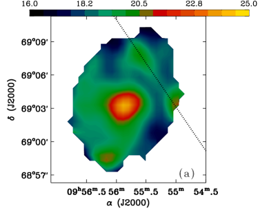
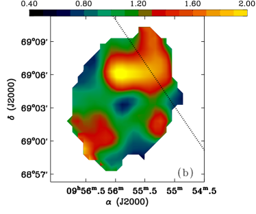
We also present the spatial distribution of dust optical depth in Fig. 5. The optical depth at 90 $\micron$ is converted to the $V$-band extinction ($A_{V}$) (Section 2.5). There is a weak anti-correlation between $A_{V}$ and $T_{\mathrm{LG}}$. The large excess of $A_{V}$ in the north-west and south-west parts of the disc may be strongly affected by the contamination of stripes caused by unstable detector response. In Fig. 5, the most prominent stripe is shown by the dotted lines indicating the scan direction. In the temperature map, there are two high-temperature islands connected with a bridge on this stripe. The neighbouring region around this line with a width of 3 arcmin may not be reliable because of some stripes. Thus, future observations of the structures around the stripes are required.

Our estimate of $A_{V}$ is reasonable if the dust in each pixel has an uniform temperature. However, in the spiral arms, as shown in the H$\alpha$ image (Fig. 1), star-forming regions whose sizes are smaller than the grid size of the FIR image are clearly seen. If the dust temperature is biased to these regions, the dust optical depth can be underestimated. In fact, as shown later in Section 4.2, the FIR colour–colour relation also supports a significant contribution of warm star-forming regions to the FIR emission in spiral arms. The central part does not show a strong indication of such inhomogeneous radiation field; that is, the dust temperature in that region might be well approximated by a single component. Thus, there is still a possibility that small $A_{V}$ in the central part is due to a deficiency of dust. However, since $A_{V}$ is very sensitive to the determination of the dust temperature and our results are affected by unstable detector response, all the features in $A_{V}$ should be confirmed by future observations.

The $A_{V}$ value is roughly 0.5–2 in the M 81 disc. Buat et al. (2005) show that FIR to ultraviolet (UV) luminosity ratio of galaxies is related to the dust extinction because the efficiency of UV reprocessing into FIR by dust is related to the dust extinction. The UV flux of M 81 at the FUV band (1528 Å) of the Galaxy Evolution Explorer (GALEX) is $F_{\nu}=179$ mJy (Dale et al., 2007). Thus, $F_{\mathit{FUV}}\equiv\nu F_{\nu}=3.51\times 10^{-9}$ erg cm^-2 s^-1. The extinction at the FUV band can be estimated by using the fitting formula derived from the model calculations by Buat et al. (2005):

$$A_{\mathit{FUV}}=-0.0333y^{3}+0.3522y^{2}+1.1960y+0.4967,$$ (5)

where $y\equiv\log(F_{\mathrm{TIR}}/F_{\mathit{FUV}})$. Using the value for $F_{\mathrm{TIR}}$ in Section 3.2, we obtain $A_{\mathit{FUV}}=1.46$. This matches the mean value for the UV-selected sample in Buat et al. (2005) in the local Universe. Now using the Galactic extinction curve given by Weingartner & Draine (2001) with $R_{V}=3.1$ ($A_{V}/A_{\mathit{FUV}}=0.389$), we obtain $A_{V}=0.57$. The extinction shown in Fig. 5 is the one over the entire column in the galactic disc. If the stars are on average located in the middle of the disc thickness, the stellar extinction would be half of the values obtained in Fig. 5; that is, $A_{V}\simeq 0.25$–1. $A_{V}=0.57$ is within this range.

4.2 Colour–colour diagram

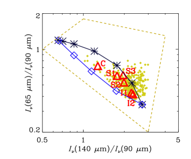
The relation among the intensities at the three bands is investigated here. Following Hibi et al. (2006), we investigate the FIR colour–colour relation. Fig. 6 shows the relation between the $65~{}\micron-90~{}\micron$ colour and the $140~{}\micron-90~{}\micron$ colour for the individual grids whose intensities are above 4 $\sigma$ of the background fluctuation for all the bands (i.e., the same criterion for the temperature map in Section 4.1). The overall trend from the lower right to the upper left can be interpreted as a sequence of dust temperature.

Now we theoretically quantify the observed colour–colour relation by adopting the calculations in Hirashita et al. (2007), who treat the dust heating by an ISRF and the dust cooling by thermal radiation to calculate the temperature distribution function using the framework developed by Draine & Li (2001). The physical quantities that explain well the dust emission properties in the solar neighbourhood are adopted: the ISRF SED by Mathis, Mezger, & Panagia (1983), the grain size distribution by Mathis, Rumpl, & Nordsieck (1977), and the heat capacity of grain materials by Draine & Li (2001). The emission coefficient of dust (silicate and graphite) are taken from Draine & Lee (1984) for $\lambda\leq 100~{}\micron$ and extrapolated by assuming a functional form proposed by Reach et al. (1995) (i.e. $\beta$ smoothly changes from 1 to 2 around $\lambda\sim 200~{}\micron$). As shown by Hirashita et al. (2007), a slight change in $\beta$ affects the colour–colour sequence significantly. To check the consistency with other nearby galaxies in the colour–colour diagram, adopting the same emission coefficient as adopted in Hirashita et al. (2007) is crucial here. We vary the ISRF with the spectral shape fixed, and denote the ISRF intensity relative to the solar neighbourhood value as $\chi$. We refer to Hirashita et al. (2007) for the details of the framework and some basic results.

We show the FIR colour–colour relation for various ISRF intensity $\chi$ in Fig. 6. We only show the results for graphite, since silicate follows the almost identical FIR colour–colour relation to graphite (Hirashita et al., 2007). We observe that the FIR colours obtained for the individual grids are roughly explained with $\chi=1$–30, although most of the points are located systematically above the theoretical predictions on the diagram. The lower values of $\chi$ correspond to the lower-$T_{\mathrm{LG}}$ regions such as interarm regions, and the higher values to the centre and the bright spots in the spiral arms.

The above theoretical colour–colour sequence is correct if the radiation field in a grid is approximated to be uniform. As clearly seen in the H$\alpha$ image in Fig. 1, there are small-scale star-forming regions, which should host warmer dust because of high radiation field intensity. In order to examine the effect of such a ‘contamination’ of warm dust, we show the FIR colour–colour relation by mixing the results with $\chi=1$ and $\chi=100$: the former value represents the general ISRF, while the latter is taken as a representative high radiation field value. The fraction of the latter (i.e. higher $\chi$) component is denoted as $f_{\mathrm{h}}$; that is, the intensity is calculated by

$$I_{\nu}=(1-f_{\mathrm{h}})I_{\nu}(\chi=1)+f_{\mathrm{h}}I_{\nu}(\chi=100),$$ (6)

where $I_{\nu}(\chi)$ is $I_{\nu}$ as a function of $\chi$. The result is shown in Fig. 6. A slight contamination of the higher-$\chi$ component with a fraction of $f_{\mathrm{h}}=0.003$ significantly lift the colour sequence upwards, explaining the upper part of the FIR colour–colour relation of the individual grids. This is because the 65 $\micron$ intensity responds most sensitively to the higher $\chi$ component. The shift of the FIR colour–colour relation by the contamination of a higher $\chi$ component is consistent with the conclusion by Hibi et al. (2006) and Hirashita et al. (2007). Hibi et al. (2006) called this upper sequence ‘sub-correlation’, and the contamination effect ‘overlap effect’.

We also compare our results with the FIR colours of the galaxies in the AKARI FIS Bright Source Catalogue in Fig. 6. The analysis of these galaxies has been done by Pollo, Rybka, & Takeuchi (2010). Since there are an enormous number of galaxies, we only show the area covered by the FIR Bright Source Catalogue galaxies. The redshifts of the sample are small and do not affect the colours. We observe that the FIR colour–colour relation in M 81 is within the consistent regime covered by the galaxy sample. Note that the FIR colours of the FIS Bright Source Catalog sample present the global colours, not those in individual regions within a galaxy. Thus, we confirm that the FIR colours of individual regions within a galaxy is fundamental in determining the global galaxy colours. The larger scatter of the FIS Bright Source Catalogue sample may be due to a larger extent of the radiation field or a peculiarity of dust emission properties in some galaxies.

In Fig. 6, we also show the colours of some representative regions within the circles of 1-arcmin radius as shown in Fig. 1: the central region (‘C’), the spiral arms (‘S1’, ‘S2’, and ‘S3’), and the interarm regions (‘I1’ and ‘I2’). We calculate the flux integrated for the circular regions, and take the flux ratios to show the colours. The fluxes are listed in Table 1. The central region have the bluest colours, while the interarm regions tend to have redder colours than the spiral arms: these trends in colours are consistent with the temperature map shown in Fig. 5. Moreover, the central and interarm regions are located relatively near to the theoretical predictions with varying ISRFs (squares in Fig. 6) on the colour–colour diagram, while the spiral arms are shifted toward the theoretical predictions with a mixture of general ISRF and a high radiation field (asterisks in Fig. 6). This indicates that the ISRF in the central and interarm regions are rather uniform and occupied with general ISRFs with different intensities, while there is a large variation in the radiation field in the spiral arms with a spatial scale well below 1 arcmin. It is probable that small star-forming regions with strong radiation fields reside in spiral arms as seen in the H$\alpha$ image (Fig. 1); this may be the reason for the mixed colour features of the spiral arms.

Figure 6: The relation between $65~{}\micron-90~{}\micron$ colour and $140~{}\micron-90~{}\micron$ colour. Small filled diamonds show the colours in the individual grids in M 81. Triangles represents the colours for the flux integrated in the regions depicted in Fig. 1. Large open diamonds present the theoretical colour–colour relation with $\chi=1$, 3, 10, 30, and 100, and asterisks show the results with $f_{\mathrm{h}}=0$, $10^{-2.5}$, $10^{-2}$, $10^{-1.5}$, $10^{-1}$, $10^{-0.5}$, and 1 from large to small $I_{\nu}(140~{}\micron)/I_{\nu}(90~{}\micron)$. The area shown by the large square with dashed lines show the representative colour–colour relations of the galaxy sample in the AKARI FIS Bright Source Catalogue (Pollo et al., 2010).

5 Discussion

5.1 FIR as a tracer of general ISRF

The dust temperature derived from the global SED (Section 3.2) is consistent with those in the interarm regions and in the smooth regions (excluding the warm spots) of the spiral arms. This suggests that the global FIR SED is more representative of the dust heated by the general ISRF rather than by the intense radiation in the star-forming regions.

That the FIR emission traces the general ISRF does not necessarily mean that the FIR traces the smoothly distributed old stellar population rather than the newly formed stellar population. It is generally hard to distinguish these two components as pointed out by Walterbos & Greenawalt (1996): An elaborated treatment of multi-wavelength star-formation indicators can be found in Hirashita, Buat, & Inoue (2003), who find that $\sim 40$ per cent of the FIR emission on average is associated with the dust heated by stellar populations older than $10^{8}$ yr in their nearby star-forming galaxy sample.

5.2 Colour–colour diagram as a diagnostics for the local heating source

The dust optical depth derived observationally depends on the structures smaller than the spatial resolution. If the ISRF is uniform in a grid used to derive the optical depth, the dust optical depth is reliable because of the dust temperature estimated represents the real dust temperature. However, if a grid is contaminated by small-scale warm spots such as a star-forming clouds, the temperature estimate is biased to such warm spots. Because of this overestimate of dust temperature, the dust optical depth can be underestimated as pointed out in Section 4.1. In other words, the FIR emission is not a good tracer of dust mass if the region focused on contains small-scale warm regions contributing significantly to the FIR emission.

We have shown in Section 4.2 that the contamination of warm regions can be identified by the FIR colour–colour diagram. As we can clearly see in Fig. 6, the spiral arms (S1, S2, and S3), which contain small-scale star-forming regions (see the H$\alpha$ image in Fig. 1), deviate from the the varying-$\chi$ sequence. The FIR colours in the spiral arms are more consistent with a mixture of a general ISRF with warm regions. Thus, we suggest that the relatively small dust optical depth in high-temperature regions of the spiral arms is due to the overestimate of dust temperature due to the contamination of warm spots possibly associated with star-forming regions (Section 4.1).

In the central region marked by ‘C’, the FIR colours are close to the point of uniform radiation field with $\chi\sim 10$. Thus, the region may be roughly approximated with a single dust temperature. If this is true, the optical depth in the central region may reflect the real optical depth; that is, the deficiency of dust optical depth in the central region with a radius of 1 arcmin (1.1 kpc) may be real. The uniformity of the radiation field also implies that the heating by AGN is not a dominant heating source in the central 1-kpc region at least for the dust which can be traced in the FIR bands. The H i gas is also deficient in the central region (Rots, 1975; Braun, 1995). Since the star formation activity in the central region is strong as seen in the H$\alpha$ image, the radiation pressure or the thermal pressure may have pushed the gas and dust outwards. If we adopt 10 km s^-1 ($\sim$ the sound velocity in the ionized regions) for the typical velocity for the gas, a structure with a size of 1.1 kpc can be formed on a time-scale of $10^{8}$ yr. Or some wave motion may be responsible for such a structure (Rots, 1975; Lowe et al., 1994).

5.3 Importance of AKARI FIS bands toward Herschel

The FIR wavelengths observed by the AKARI FIS bands (50–180 $\micron$) cover the intensity peak of the FIR SED. This means that the intensities in the AKARI FIS bands depends both on the wavelength and the dust temperature in a strongly nonlinear way. This strong nonlinearity is important in the behaviour in the colour–colour diagram: not only the strong dependence on $\chi$ but also the large separation of the two sequences (i.e. varying $\chi$ and varying $f_{\mathrm{h}}$) is due to such a nonlinearity. Moreover, the three (in fact four) bands available for AKARI FIS have advantage in the colour–colour analysis.

Herschel is also suitable for the aim of mapping dust emission in galaxies. In spite of its higher spatial resolution, the warm spots associated with star-forming regions cannot be resolved at the distance of M 81. Thus, the only way to show the existence of such warm spots in the FIR is to plot the FIR colours (Section 5.2). Recently, Bendo et al. (2010) have observed M 81 with Herschel over a wide wavelength range of 70–500 $\micron$. The peak of the SED is at $\lambda\la 160\,\micron$ for $T_{\mathrm{LG}}\ga 20$ K. Thus, the Herschel PACS 100 $\micron$ and 160 $\micron$ bands (Poglitsch et al., 2010) are suitable for covering the peak. The fact that similar temperatures are derived by both AKARI and Herschel (29 K, 20 K, 17 K for the nucleus, arm, and interarm, respectively; Bendo et al. 2010) indicates that the FIR SED can be interpreted consistently from 90 $\micron$ to 500 $\micron$ with a single temperature. Note that even with the Herschel higher resolution data, AKARI data still have an advantage that an enormous number of the AKARI All-Sky Survey data are available for a comparison at the same wavelengths (Section 4.2).

6 Conclusion

We have investigated the properties of FIR emission in a spiral galaxy, M 81, by utilizing the AKARI imaging data at 65, 90, and 140 $\micron$. Combining the images in the two long-wavelength bands (90 and 140 $\micron$), we have derived the dust temperature map. The dust temperature is $\sim 25$ K in the centre and becomes lower in the outer part. The dust temperature derived from the global 90 and 140 $\micron$ intensities is $T_{\mathrm{LG}}=18.6^{+1.9}_{-1.6}$ K, which reflects the dust temperatures in the interarm regions or the spiral arms excluding the bright knots, rather than those in the centre or in the bright knots. Thus, the global dust temperature is more representative of the dust heated by the general ISRF. We have also shown the 140 $\micron$ emission is more radially extended than the 90 $\micron$ emission, which is consistent with the radial dust temperature gradient. The dust optical depth traced by the FIR emission is $A_{V}=0.5$–2. If these values are divided by 2 with an assumption that the stars are in the mid-plane on average, the expected extinction for the stellar light is $A_{V}=0.25$–1, consistent with the the extinction derived from the FIR-to-UV ratio ($A_{V}=0.57$).

We have also demonstrated that the FIR colour–colour diagram is a useful tool to distinguish whether or not individual regions within a galaxy is dominated by a smooth ISRF or contaminated by warm spots associated with star-forming regions. Based on this ‘tool’, we conclude that the bright regions in the spiral arms contain small-scale warm regions possibly hosting the H ii regions seen in the H$\alpha$ map. This contamination of warm regions causes an underestimate of dust optical depth (or dust column density).

Since even Herschel cannot resolve individual star-forming regions, the FIR colour–colour diagram continues to be a useful tool to see if the dust is predominantly heated by a general ISRF or the dust heating by individual star-forming regions affects the FIR emission.

References

- Aannestad & Kenyon (1979) Aannestad, P. A., & Kenyon, S. J. 1979, ApJ, 230, 771
- Baggett, Baggett, & Anderson (1998) Baggett, W. E., Baggett, S. M., & Anderson, K. S. J. 1998, ApJ, 116, 1626
- Bendo et al. (2010) Bendo, G., et al. 2010, A&A, 518, L65
- Braun (1995) Braun, R. 1995, A&AS, 114, 409
- Buat et al. (2005) Buat, V., et al. ApJ, 619, L51
- Cheng et al. (1997) Cheng, K.P., Collins, N., Angione, R., Talbert, F., Hintzen, P., Smith, E. P., Stecher, T., & The UIT Team, Uv/visible Sky Gallery on CDROM
- Dale et al. (2001) Dale, D. A., Helou, G., Contursi, A., Silbermann, N. A., & Kolhatkar, S. 2001, ApJ, 549, 215
- Dale et al. (2007) Dale, D. A., et al. 2007, ApJ, 655, 863
- Draine & Anderson (1985) Draine, B. T., & Anderson, N. 1985, ApJ, 292, 494
- Draine & Lee (1984) Draine, B. T., & Lee, H. M. 1984, ApJ, 285, 89
- Draine & Li (2001) Draine, B. T., & Li, A. 2001, ApJ, 551, 807
- Freedman et al. (1994) Freedman, W. L., et al. 1994, ApJ, 427, 628
- Harper & Low (1973) Harper, D. A., Jr., & Low, F. J. 1973, ApJ, 182, L89
- Hibi et al. (2006) Hibi, Y., Shibai, H., Kawada, M., Ootsubo, T., & Hirashita, H. 2006, PASJ, 58, 509
- Hirashita, Buat, & Inoue (2003) Hirashita, H., Buat, V., & Inoue, A. K. 2003, A&A, 410, 83
- Hirashita et al. (2007) Hirashita, H., Hibi, Y., & Shibai, H. 2007, MNRAS, 379, 974
- Hirashita et al. (2008) Hirashita, H., Kaneda, H., Onaka, T., & Suzuki, T. 2008, PASJ, 60, S477
- Inoue, Hirashita, & Kamaya (2000) Inoue, A. K., Hirashita, H., & Kamaya, H. 2000, PASJ, 52, 539
- Kawada et al. (2007) Kawada, M., et al. 2007, PASJ,, 59, S389
- Kennicutt (1998) Kennicutt, R. C., Jr. 1998, ARA&A, 36, 189
- Li & Draine (2001) Li, A., & Draine, B. T. 2001, ApJ, 554, 778
- Lowe et al. (1994) Lowe, S. A., Roberts, W. W., Yang, J., Bertin, G., & Lin, C. C. 1994, ApJ, 427, 184
- Mathis, Rumpl, & Nordsieck (1977) Mathis, J. S., Rumpl, W., & Nordsieck, K. H. 1977, ApJ, 217, 425
- Mathis, Mezger, & Panagia (1983) Mathis, J. S., Mezger, P. G., & Panagia, N. 1983, A&A, 128, 212
- Murakami et al. (2007) Murakami, H., et al. 2007, PASJ, 59, S369
- Nagata et al. (2002) Nagata, H., Shibai, H., Takeuchi, T. T., & Onaka, T. 2002, PASJ, 54, 695
- Pérez-González et al. (2006) Pérez-González, P. G., et al. 2006, ApJ, 648, 987
- Pilbratt et al. (2010) Pilbratt, G. L., et al. 2010, A&A, 518, L1
- Poglitsch et al. (2010) Poglitsch, A., et al. 2010, A&A, 518, L2
- Pollo et al. (2010) Pollo, A., Rybka, P., & Takeuchi, T. T. 2010, A&A, 514, A3
- Reach et al. (1995) Reach, W. T. et al., 1995, ApJ, 451, 188
- Rice et al. (1988) Rice, W., Lonsdale, C. J., Soifer, B. T., Neugebauer, G., Kopan, E. K., Lloyd, L., de Jong, T., & Habing, H. J. 1988, ApJS, 68, 91
- Rots (1975) Rots, A. H. 1975, A&A, 45, 43
- Sauvage et al. (2010) Sauvage, M., et al. 2010, A&A, 518, L64
- Shibai, Okumura, & Onaka (1999) Shibai, H., Okumura, K., & Onaka, T. 1999, in Nakamoto T. ed., Star Formation 1999, Nobeyama Radio Observatory, Nobeyama, p. 67
- Shirahata et al. (2008) Shirahata, M., et al. 2008, PASJ, 61, 737
- Suzuki et al. (2007) Suzuki, T., Kaneda, H., Nakagawa, T., Makiuti, S., & Okada, Y. 2007, PASJ, 59, S473
- Suzuki et al. (2010) Suzuki, T., Kaneda, H., Onaka, T., Nakagawa, T., & Shibai, H. 2010, A&A, in press (arXiv: 1006.2018)
- Takeuchi et al. (2010) Takeuchi, T. T., Buat, V., Heinis, S., Giovannoli, E., Yuan, F.-T., Iglesias-Páramo, J., Murata, K. L., Burgarella, D. 2010, A&A, 514, A4
- Verdugo et al. (2007) Verdugo, E., Yamamura, I., & Pearson C. P., 2007, AKARI FIS Data User Manual Version 1.3 (http://www.ir.isas.ac.jp/ASTRO-F/Observation/)
- Walterbos & Greenawalt (1996) Walterbos, R. A. M., & Greenawalt, B. 1996, ApJ, 460, 696
- Weingartner & Draine (2001) Weingartner, J. C., & Draine, B. T. 2001, ApJ, 548, 296
- Yamamura et al. (2009) Yamamura, I., et al. 2009, in Onaka T., White G., Nakagawa T., Yamamura I. ed., ASP Conf. Ser. Vol. 418, AKARI, a Light to Illuminate the Misty Universe. Astron. Soc. Pac., San Francisco, p. 3