Computational Complexity of Avalanches in the Kadanoff two-dimensional Sandpile Model

Abstract

In this paper we prove that the avalanche problem for Kadanoff sandpile model (KSPM) is P-complete for two-dimensions. Our proof is based on a reduction from the monotone circuit value problem by building logic gates and wires which work with configurations in KSPM. The proof is also related to the known prediction problem for sandpile which is in NC for one-dimensional sandpiles and is P-complete for dimension $3$ or greater. The computational complexity of the prediction problem remains open for two-dimensional sandpiles.

1 Introduction

Predicting the behavior of discrete dynamical systems is, in general, both the “most wanted” and the hardest task. Moreover, the difficulty does not decrease when considering finite phase spaces. Indeed, when the system is not solvable, numerical simulation is the only possibility to compute future states of the system.

In this paper we consider the well-known discrete dynamical system of sandpiles (SPM). Roughly speaking, its dynamics is as follows. Consider the toppling of grains of sand on a (clean) flat surface, one by one. After a while, a sandpile has formed. At this point, the simple addition of even a single grain may cause avalanches of grains to fall down along the sides of the sandpile. Then, the growth process of the sandpile starts again. Remark that this process can be naturally extended to arbitrary dimensions although for $d>3$, the physical meaning is not clear.

The first complexity results about SPM appeared in  [6, 7] where the authors proved the computation universality of SPM. For that, they modelled wires and logic gates with sandpiles configurations. Inspired by these constructions, C. Moore and M. Nilsson considered the prediction problem (PRED) for SPM i.e. the problem of computing the stable configuration (fixed point) starting from a given initial configuration of the sandpile. C. Moore and M. Nilsson proved that PRED is in $\textsf{NC}^{3}$ for dimension $1$ and that it is P-complete for $d\geq 3$ leaving $d=2$ as an open problem [12]. (Recall that P-completeness plays for parallel computation a role comparable to NP-completeness for non-deterministic computation. It corresponds to problems which cannot be solved efficiently in parallel (see [9]) or, equivalently, which are inherently sequential). Later, P.B. Miltersen improved the bound for $d=1$ showing that PRED is in LOGDCFL ($\subseteq\textsf{AC}^{1}$) and that it is not in $\textsf{AC}^{1-\epsilon}$ for any $\epsilon>0$ [11]. Therefore, in any case, one-dimensional sandpiles are capable of (very) elementary computations such as computing the max of $n$ bits.

Both C. Moore and P.B. Miltersen underline that

‘‘having a better upper-bound than P for PRED for two-dimensional sandpiles would be most interesting.”

In this paper, we address a slightly different problem: the avalanche problem (AP). Here, we start with a monotone configuration of the sandpile. We add a grain of sand to the initial pile. This eventually causes an avalanche and we address the question of the complexity of deciding whether a certain given position –initially with no grain of sand– will receive some grains in the future. Like for the (PRED) problem, (AP) can be formulated in higher dimensions. In order to get acquainted with AP, we introduce its one-dimensional version first.

One-dimensional sandpiles can be conveniently represented by a finite sequence of integers $x_{1},x_{2},\ldots,x_{k},\ldots,x_{n}$. The sandpiles are represented as a sequence of columns and each $x_{i}$ represents the number of grains contained in column $i$. In the classical SPM, a grain falls from column $i$ to $i+1$ if and only if the height difference $x_{i}-x_{i+1}\geq 2$. Kadanoff’s sandpile model (KSPM) generalizes SPM [10, 5] by adding a parameter $p$. The setting is the same except for the local rule: one grain falls to the $p-1$ adjacent columns if the difference between column $i$ and $i+1$ is greater than $p$.

Assume $x_{k}=0$, for a value of $k$ “far away” from the sandpile. The avalanche problem asks whether adding a grain at column $x_{1}$ will cause an avalanche such that at some point in the future $x_{k}\geq 1$, that is to say that an avalanche is triggered and reaches the “flat” surface at the bottom.

This problem can be generalized for two-dimensional sandpiles and is related to the question addressed by C. Moore and P.B. Miltersen.

In this paper we prove that in the two-dimensional case, AP is P-complete. The proof is obtained by reduction from the Circuit Value Problem where the circuit only contains monotone gates — that is, AND’s and OR’s (see section 3 for details).

We stress that our proof for the two-dimensional case needs some further hypothesis/constraints for monotonicity and determinism (see section 3). If both properties are technical requirements for the proof’s sake, monotonicity also has a physical justification. Indeed, if KSPM is used for modelling real physical sandpiles, then the image of a monotone non-increasing configuration has to be monotone non-increasing since gravity is the only force considered here. We have chosen to design the Kadanoff automaton for $d=2$ by considering a certain definition of the three-dimensional sandpile which does not correspond to the one of Bak’s et al. in [1]. This hypothesis is not restrictive. It is just used for constructing the transition rules. Bak’s construction was done similarly. Nevertheless, our result depends on the way the three dimensional sandpile is modelled. In our case, we have decided to formalise the sandpile as a monotone decreasing pile in three dimensions where $x_{i,j}\geq\max\{x_{i+1,j},x_{i,j+1}\}$ (here $x_{i,j}$ denotes the sand grains initial distribution) together with Kadanoff’s avalanche dynamics ruled by parameter $p$. The pile $(i,j)$ can give a grain either to every pile $(i+1,j),\ldots,(i+p-1,j)$ or to every pile $(i,j+1),\ldots,(i,j+p-1)$ if the monotonicity is not violated. With such a rule and if we use the height difference for defining the monotonicity, we can define the transition rules of the automaton for every value of the parameter $p$.

In the case where the value of the parameter $p$ equals $2$, we find in our definition of monotonicity something similar with Bak’s SPM in two dimensions. Actually, both models are different because the definitions of the three dimensional piles differ. That is the reason why we succeed in proving the P-completeness result which remains an open problem with Bak’s definition.

The paper is organized as follows. Section 2 introduces the definitions of the Kadanoff sandpile model in one dimension and presents the avalanche problem. Section 3 generalizes the Kadanoff sandpile model in two dimensions and presents the avalanche problem in two dimension, which is proved P-complete for any value of the Kadanoff parameter $p$. Finally, section 4 concludes the paper and proposes further research directions.

2 Sandpiles and Kadanoff model in one dimension

A sandpile configuration is a distribution of sand grains over a lattice (here $\mathbb{Z}$). Each site of the lattice is associated with an integer which represents its sand content. A configuration is finite if only a finite number of sites has non-zero sand content. Therefore, in the sequel, a finite configuration on $\mathbb{Z}$ will be identified with an ordered sequence of integers $x_{1},x_{2},\ldots,x_{n}$ in which $x_{1}$ (resp. $x_{n}$) is the first (resp. the last) site with non-zero sand content. A configuration $x$ is monotone if $\forall i\in\mathbb{Z}$, $x_{i}\geq x_{i+1}$. A configuration $x$ is stable if $\forall i\in\mathbb{Z}$, $x_{i}-x_{i+1}<p$ i.e. if the difference between any two adjacent sites is less than Kadanoff’s parameter $p$. Let SM$(n)$ denote the set of stable monotone configurations of the form ${}^{\omega}x_{1},x_{2},\ldots,x_{n-1},x_{n}^{\omega}$ and of length $n$, for $x_{i}\in\mathbb{N}$.

Given a configuration $x$, $a\in\mathbb{N}$ and $j\in\mathbb{Z}$, we use the notation ${}^{\omega}ax_{j}$ (resp. $x_{j}a^{\omega}$) to say that $\forall i\in\mathbb{Z}$, $i<j\rightarrow x_{i}=a$ (resp. $\forall i\in\mathbb{Z}$, $i>j\rightarrow x_{i}=a$).

Finally, remark that any configuration ${}^{\omega}x_{1},x_{2},\ldots,x_{n-1},x_{n}0^{\omega}$ can be identified with its height difference sequence ${}^{\omega}0,(x_{1}-x_{2}),\ldots,(x_{n-1}-x_{n}),x_{n},0^{\omega}$  .

Consider a stable monotone configuration ${}^{\omega}x_{1},x_{2},\dots,x_{n}^{\omega}$. Adding one more sand grain, say at site $i$, may cause that the site $i$ topples some grains to its adjacent sites. In their turn the adjacent sites receive a new grain of sand and may also topple, and so on. This phenomenon is called an avalanche. The avalanche ends when the system evolves to a new stable configuration.

Figure 1: Avalanches for $p=3$ with 9 columns. Here, $x_{i}+1$ (resp. $x_{i}+2$) indicates that column $i$ has received some grains once (resp. twice), $x_{i}-1$ that column $i$ has given some grains according to the dynamics; a dark shaded site indicates the toppling site, a light shaded site indicates a site that could topple in the future. Times goes top-down.

In this paper, topplings are controlled by the Kadanoff’s parameter $p\in\mathbb{N}$ which completely determines the model and its dynamics. In KSPM$(p)$, $p-1$ grains will fall from site $i$ if $x_{i}-x_{i+1}\geq p$ and the new configuration becomes

$${}^{\omega}x_{1}\cdots(x_{i-1})(x_{i}-p+1)(x_{i+1}+1)\cdots(x_{i+p-2}+1)(x_{i+p-1}+1)(x_{i+p})\cdots x_{n}0^{\omega}\enspace.$$

In other words, the site $i$ distributes one grain to each of its $(p-1)$ right adjacent sites. Equivalently, if we mesure the height differences after applying the dynamics, we get $(h_{i-1}+p-1)(h_{i}-p)(h_{i+1})(h_{i+2})\cdots(h_{i+p-2})(h_{i+p-1}+1)\enspace,$ where $h_{i-1}=(x_{i-1}-x_{i})$ and all remaining heights do not change. In other words, the height difference $h_{i}$ gives rise to an increase of $(p-1)$ grains of sand to height $h_{i-1}$ and an increase of one grain to height $h_{i+p-1}$.

We consider the problem of deciding whether some column on the right of column $x_{n}$ (more precisely for column $x_{k}$ for $n<k\leq n+p-1$) will receive some grains according to the Kadanoff’s dynamics. Since the initial configuration is stable, it is not difficult to prove that avalanches will reach at most the column $n+p-1$ (see figure 1 for example).

Remark that given a configuration, several sites could topple at the same time. Therefore, at each time step, one might have to decide which site or which sites are allowed to topple. According to the update policy chosen, there might be different images of the same configuration. However, it is known  [8] that for any given initial number of sand grains $n$, the orbit graph is a lattice and hence, for our purposes, we may only consider one decision problem to formalize AP:

Problem AP

Instance

A configuration $x\in$ SM$(n)$ and $k\in\mathbb{N}$ s.t. $n\!<k\!\leq n+p-1$

Question

Does there exist an avalanche such that $x_{k}\geq 1$?

Let us consider some examples. Let $p=3$ and consider a stable bi-infinite configuration such that its height differences is as follows ${}^{\omega}00\underline{2}2022120000^{\omega}$. We add just one grain at $x_{1}$ (the site underlined in the configuration). Then, the next step is ${}^{\omega}02\underline{0}21222120000^{\omega}$. And so in one step we see that no avalanche can be triggered, hence the answer to $AP$ is negative. As a second example, consider the following sequence of height differences (always with $p=3$): ${}^{\omega}0\underline{3}122122221201200^{\omega}$. There are several possibilities for avalanches from the left to the right but none of them arrives to the 0’s region. So the answer to the decision problem is still negative. To get an idea of what happens for a positive instance of the problem, consider the following initial configuration: ${}^{\omega}0\underline{3}12222100^{\omega}$ with parameter $p=3$.

The full proof of Theorem 2.1 is a bit technical and will be given in the journal version of the paper.

Theorem 2.1

AP is in $\textsf{NC}^{1}$ for KSPM in dimension $1$ and $p>1$.

Proof (Sketch of the proof.)

The first step is to prove that, in this situation, the Kadanoff’s rule can be applied only once at each site for any initial monotone stable configuration. Using this result one can see that a site $k$ such that $x_{k}=0$ in the initial configuration and $x_{k}>1$ in the final one, must have received grains from site $k-p$. This site, in its turn, must have received grains from $k-2p$ and so on until a “firing” site $i$ with $i\in[\![1,p-1]\!]$. The height difference for all of these sites must be $p-1$. The existence of this sequence and the values of the height differences can be checked by a parallel iterative algorithm on a PRAM in time $\mathcal{O}\left(\log n\right)$.

3 Sandpiles and Kadanoff model in two dimensions

There are several possibilities to define extensions of the Kadanoff dynamics to two dimensional sandpiles. Let us first extend the basic definitions introduced in section 2.

A two-dimensional sandpile configuration is a distribution of grains of sand over the $\mathbb{N}\times\mathbb{N}$ lattice. As in the one-dimensional case, a configuration is finite if only a finite number of sites has non-zero sand content. Therefore, in the sequel, a finite configuration on $\mathbb{N}\times\mathbb{N}$ will be identified by a mapping from $\mathbb{N}\times\mathbb{N}$ into $\mathbb{N}$, giving a number of grains of sand to every position in the lattice. Thus, a configuration will be denoted by $x_{i,j}$ as $(i,j)\mapsto\mathbb{N}$. A configuration $x$ is monotone if $\forall i,j\in\mathbb{N}\times\mathbb{N}$, $x_{i,j}$ is such that $x_{i,j}\geq 0$ and $x_{i,j}\geq\max\{x_{i+1,j},x_{i,j+1}\}$. So we have a monotone sandpile, in the same sense as in [2]. A configuration $x$ is horizontally stable (resp. vertically) if $\forall i,j\in\mathbb{N}\times\mathbb{N},\quad x_{i,j}-x_{i+1,j}<p$ (resp. $\forall i,j\in\mathbb{N}\times\mathbb{N},\quad x_{i,j}-x_{i,j+1}<p$) and is stable if it is both horizontally and vertically stable. In other words, it is a generalisation of the Kadanoff model in one dimension, that is the configuration is stable if the difference between any two adjacent sites is less than the Kadanoff parameter $p$. To this configuration, we apply the Kadanoff dynamics for a given integer $p\geq 1$. The application can be done if and only if the new configuration remains monotone. Example 1 illustrates the case which violates the condition of monotonicity of the Kadanoff dynamics.

Example 1

Consider the initial configuration given in the bottom left matrix of the following figure

$$\begin{array}[]{ccc}\begin{matrix}0&1&0&0\\ \boxed{2}&3&0&0\\ 8&4&2&2\\ 8&4&3&2\end{matrix}&&\\ &&\\ \uparrow v&&\\ &&\\ \begin{matrix}0&0&0&0\\ 2&2&0&0\\ 8&\boxed{6}&2&2\\ 8&4&3&2\end{matrix}&\stackrel{{\scriptstyle h}}{{\rightarrow}}&\begin{matrix}0&0&0&0\\ 2&2&0&0\\ 8&4&3&\boxed{3}\\ 8&4&3&2\end{matrix}\\ \end{array}$$

Values count for the number of grains of a site. We see that we cannot apply the Kadanoff’s dynamics for a value of parameter $p=3$ from the boxed site. Indeed, the resulting configurations do not remain monotone neither by applying the dynamics horizontally nor vertically (resp. $\uparrow\!v$ and $\stackrel{{\scriptstyle h}}{{\rightarrow}}$). A site which violates the condition has been boxed in the resulting configurations (it might be not unique).∎

Recall that the Kadanoff operator applied to site $(i,j)$ for a given $p$ consists in giving a grain of sand to any site in the horizontal or vertical line, i.e $\{(i,j+1),....(i,j+p-1)\}$ or $\{(i+1,j),...(i+p-1,j)\}$.

Similarly to the one-dimensional case, we associate to the previous avalanches their height difference. Any configuration can be identified by the mapping of its horizontal height difference (resp. vertical): $h_{\rightarrow}:(i,j)\mapsto x_{i,j}-x_{i+1,j}$ (resp. $h_{\uparrow}:(i,j)\mapsto x_{i,j}-x_{i,j+1}$). The height difference allows to define the notions of monotonicity and stability in a straightforward way. However, notice that when considering the dynamics defined over height differences, we work with a different lattice though isomorphic to the initial one. The relationship between them is depicted on figure 4.

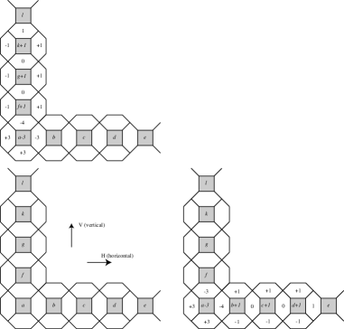
Figure 2: Horizontal and vertical chenilles for $p=4$. Shaded squares count the number of grains on each column and the hexagons between the squares the height difference between the corresponding two adjacent columns. The initial configuration is on the bottom-left. The Kadanoff’s dynamics is applied from the shaded site labelled $a$ horizontally or vertically (resp. $\uparrow\!V$ and $\stackrel{{\scriptstyle H}}{{\rightarrow}}$) to get the resulting configurations.

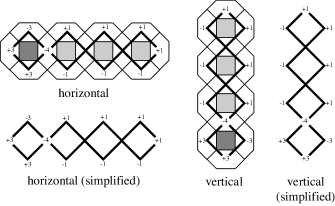
Figure 3: Horizontal and vertical chenilles for $p=4$. The dynamics is applied to the dark-shaded site (the leftmost one on the left part of the figure and the lowest one on the right part of the figure). The numbers express the height differences after the application of the dynamics. The two simplified views remove the number of sand grains information and only keeps the height difference information. It corresponds to a change in the lattice structure if the grains are considered or the height difference.

For a better understanding of the dynamics, recall that in one dimension an avalanche at site $i$ changes the heights of sites $i-1$ and $i+p-1$. In two dimensions, there are height changes on the line but also to both sides of it. The dynamics is simpler to depict than to write it down formally. It will be presented throughout examples and figures in the sequel. An example of the Kadanoff’s dynamics applied horizontally (resp. vertically) is given in figure 2. More precisely, the Kadanoff’s dynamics for a value of parameter $p=4$ is depicted in figure 3. Observe that we do not need to take into account the number of grains of sand in the columns. It sufficies to take the graph of the edges adjacent to each site (depicted by thick lines) and to store the height differences. So, from now on, we will restrict ourselves to the lattice and to the dynamics defined on the height differences. In figure 3, we only keep the information required for applying the dynamics in the simplified view. In fact, the local function is depicted by figure 4 that we will call Chenilles (horizontal and vertical, respectively).

Figure 4 explains how the dark site with coordinates $(i,j)$ with a height difference of $p$ gives grains either horizontally (figure 4 left) or vertically (figure 4 right).

Example 2 (Obtaining Bak’s)

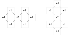
Figure 5: Templates for Bak’s dynamics with $p=2$.

In the case $p=2$ and if we assume the real sandpile is defined as in [2] (i.e. $x_{i,j}\geq\max\{x_{i+1,j},x_{i,j+1}\}$), we get the templates from figure 5.∎

In order to be applied, the automaton’s dynamics requires to test if the local application gives us a non-negative configuration.

3.1 P-completeness

Changing from dimension $1$ to $2$ (or greater), the statement of AP has to be adapted. Consider a finite configuration $x$ which is non-zero for sites $(i,j)$ with $i,j\geq 0$, stable and monotone and let $Q$ be the sum of the height differences. Let us denote by $n$ the maximum index of non-zero height differences along both axis. Then, SM$(n)$ denotes the set of monotone stable configurations of the form given by a lower-triangular matrix of size $n\times n$. To generalise the avalanche problem in two dimensions, we have to find a generic position which is far enough from the initial sandpile but close enough to be attained. To get rough bounds, we have followed the following approach. For the upper bound, the worst case occurs when all the grains are arranged on a single site (with a height difference of $Q$) which is at an end of one of the axis and they fall down. For the lower bound, it is the same reasoning, except that the pile containing the grains is at the origin. Thus, we may restate our decision problem as follows:

Problem AP (dimension 2)

Instance

A configuration $x\in$ SM$(n)$, $(k,\ell)\in\mathbb{N}\times\mathbb{N}$ such that $x_{k,\ell}=0$ and $\frac{\sqrt{2}}{2}n\leq\|(k,\ell)\|\leq n+Q$ (where $Q$ is the sum of the height differences).

Question

Does there exist an avalanche (obtained by using the vertical and horizontal chenilles) such that $x_{k,\ell}\geq 1$?

where $\|.\|$ denotes the standard Euclidean norm.

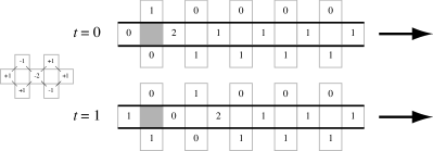
Figure 7: Information propagation in a wire for $p=2$ at times $t=0$ and $t=1$ using the templates for Baks dynamics (recalled on the left of the figure).

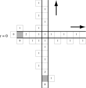
Figure 8: Crossing over two wires for $p=2$; arrows show the directions of propagation.

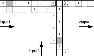
Figure 9: A logic AND gate with two inputs for $p=2$. The upcoming “2” has to reach the horizontal “2” to change the value of the boxed “0” to “1”. Then, the upcoming “2” can apply the vertical chenille template and changes the circled “1” into “2”. In other words, the AND is computed by applying 3 horizontal chenilles and 4 vertical ones.

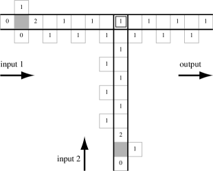
Figure 10: A logic OR gate with two inputs for $p=2$. The boxed cell indicates the OR gate point of computation.

To prove the P-completeness of AP we will proceed by reduction from the monotone circuit value problem (MCVP), i.e given a circuit with $n$ inputs $\{\alpha_{1},...,\alpha_{n}\}$ and logic gates AND, OR we want to answer if the output value is one or zero (refer to [9] for a detailed statement of the problem). NOT gates are not allowed but the problem remains P-complete for the following reason: using De Morgan’s laws $\overline{a\wedge b}=\overline{a}\vee\overline{b}$ and $\overline{a\vee b}=\overline{a}\wedge\overline{b}$, one can shift negation back through the gates until they only affect the inputs themselves. For the reduction, we have to construct, by using sandpile configurations, wires (figure 7), logic AND gates (figure 9), logic OR gates (figure 10), cross-overs (figure 8) and signal multipliers for starting the process (figure 11). We also need to define a way to deterministically update the network; to do this, we can apply the chenille’s templates any way such that it is spatially periodical, for instance from the left to the right and from the top to the bottom. Our main result is thus:

Theorem 3.1

$AP$ is P-complete for KSPM in dimension two and any $p\geq 2$.

Proof

The fact that our problem is in P is already known since C. Moore and M. Nilsson paper [12]. The proof is done by proving that the total number of avalanches required to relax a sandpile is polynomial in the system size. The remaining open problem in their study was the case $d=2$ for which they wrote “The reader may […] find a clever embedding of non-planar Boolean circuits”, which is precisely what will be done hereafter. For the reduction, one has to take an arbitrary instance of (MCVP) and to build an initial configuration of a sandpile for the Kadanoff’s dynamics for $p=2$ (or greater). Remark that, in the case $p=2$, KSPM corresponds to Bak’s model [1] in two dimensions with a sandpile such that $x_{i,j}\geq\max\{x_{i+1,j},x_{i,j+1}\}$. To complete the proof, we have to design:

• a wire (figure 7);

• the crossing of information (figure 8);

• a AND gate (figure 9);

• a OR gate (figure 10);

• a signal multiplier (figure 11).

The construction is shown graphically for $p=2$ but can be done for greater values. For $p=2$, the horizontal and vertical chenilles are given in figure 5. According to [4], the reduction is in NC since MCVP is logspace complete for P. Recall that the decision problem only adds a sand grain to one site, say $(0,0)$. To construct the entry vector to an arbitrary circuit we have to construct from the starting site wires to simulate any variable $\alpha_{i}=1$. (If $\alpha_{i}=0$ nothing is done: we do not construct a wire from the initial site. Else, there will be a wire to simulate the value 1).

Remark 1

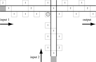
Figure 6: The logic AND gate for two inputs for $p=3$. The circled “2” is put in order to get enough tokens for the horizontal and vertical inputs.

For $p\geq 3$, the construction of the AND gate is easier than for $p=2$. The dynamics is obtained from figure 4 and the construction of an AND gate is depicted on figure 6.

4 Conclusion and future work

We have proved that the avalanche problem for the KSPM model in two dimensions is P-complete with a sandpile defined as in [2] and for every value of the parameter $p$. Let us also point out that in the case where $p=2$, this model corresponds to the two dimensional Bak’s model with a pile such that $x_{i,j}\geq 0$ and $x_{i,j}\geq\max\{x_{i+1,j},x_{i,j+1}\}$. In this context, we also proved that this physical version (with a two dimension sandpile interpretation) is P-complete. It is important to notice that, by directly taking the two dimensional Bak’s tokens game (given a graph such that a vertex has a number of token greater or equal than its degree, it gives one token to each of its neighbors), its computation universality was proved in [7] by designing logical gates in non-planar graphs. Furthermore, by using the previous construction, C. Moore et al. proved the P-completeness of this problem for lattices of dimensions $d$ with $d\geq 3$. But the problem remained open for two dimensional lattices. Furthermore, it was proved in [3] that, in the above situation, it is not possible to build circuits because the information is impossible to cross. The two dimensional Bak’s operator corresponds, in our framework, to the application of the four rotations of the template (see figure 12). But this model is not anymore the representation of a two dimensional sandpile as presented in [2], that is with $x_{i,j}\geq 0$ and $x_{i,j}\geq\max\{x_{i+1,j},x_{i,j+1}\}$.

To define a reasonable two dimensional model, consider a monotone sandpile decreasing for $i\geq 0$ and $j\geq 0$. Over this pile we define the extended Kadanoff’s model as a local avalanche in the growing direction of the $i-j$ axis such that monotonicity is allowed. Certainly, one may define other local applications of Kadanoff’s rule which also match with the physical sense of monotonicity. For instance, by considering the set ${(i+1,j),(i+1,j+1),(i,j+1)}$ as the sites to be able to receive grains from site $(i,j)$. In this sense it is interesting to remark that the two dimensional sandpile defined by Bak (i.e for nearest neighbors, also called the von Neumann neihborhood, a site gives a token to each of its four neighbors if and only if it has enough tokens) can be seen as the application of the Kadanoff rule for $p=2$ by applying to a site, if there are at least four tokens, the horizontal $(\rightarrow)$ and the vertical $(\downarrow)$ chenille simultaneoulsly (see figure 12). Similarily, for an arbitrary $p$, one may simultaneously apply other conbinations of chenilles which, in general, allows us to get P-complete problems. For instance, when there are enough tokens, the applications of the four chenilles (i.e. $\leftarrow$,$\rightarrow$,$\uparrow$ and $\downarrow$) gives raise to a new family of local templates called butterflies (because of their four wings). It is not so difficult to construct wires and circuits for butterflies. Hence, for this model of sandpiles, the decison problem will remain P-complete. One thing to analyze from an algebraic and complexity point of view is to classify every local rule derivated from the chenille application. Further, one may define a more general sandpile dynamics which contains both Bak’s and Kadanoff’s ones: i.e given an integer $p\geq 2$, we allow the application of every Kadanoff’s update for $q\leq p$. We are studying this dynamics and, as a first result, we observe yet that in one dimension there are several fixed points and also, given a monotone circuit with depth $m$ and with $n$ gates, we may simulate it on a line with this generalized rule for a given $p\geq m+n$.

For the one-dimensional avalanche problem as defined in section 2, it can be proved that it belongs tho the class NC for $p=2$ and that it remains in the same class when the first $p$ columns contain more than one grain (i.e. that there is no hole in the pile). We are in the way to prove the same in the general case.

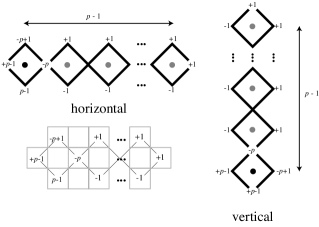
Figure 4: Horizontal resp. vertical (on the left resp. on the right) chenilles in the $\mathbb{N}\times\mathbb{N}$ lattice for arbitrary parameter $p\geq 2$. The site $(i,j)$ –denoted by a black bullet– gives one grain of sand to the site $(i+p-1,j)$ horizontally resp. one grain of sand to the site $(i,j+p-1)$ vertically. The figure gives the height differences of this dynamics and the change of the lattice structure between the dynamics on the grains and the corresponding dynamics on the height difference. In the sequel, we will adopt the representation on the left and on the bottom for defining the templates.

Figure 11: A signal multiplier for $p=2$. The signal starts on boxed site with value 2 and the first vertical chenille ruled by the Kadanoff’s dynamics multiplies the signal on both horizontal wires.

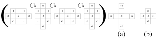
Figure 12: From Bak’s to Kadanoff’s operators. All the Kadanoff’s operators between the brackets have been applied to get the pattern (a). The Bak’s pattern (b) is obtained by eliminating the holes in (a) and by dividing the number of tokens by two.

References

- [1] P. Bak, C. Tang, and K. Wiesenfeld. Self-organized criticality. Phys. Rev. A, 38(1):364–374, 1988.
- [2] E. Duchi, R. Mantaci, H. Duong Phan, and D. Rossin. Bidimensional sand pile and ice pile models. Pure Math. Appl. (PU.M.A.), 17(1-2):71–96, 2006.
- [3] A. Gajardo and E. Goles. Crossing information in two dimensional sand piles. Theoretical Computer Science, 369(1-3):463–469, 2006.
- [4] L.M. Goldschlager. The monotone and planar circuit value problems are log space complete for P. ACM sigact news, 9(2):25–29, 1977.
- [5] E. Goles and M. Kiwi. Sand pile dynamics in one dimensional bounded lattice. In N. Boccara et al, editor, Cellular Automata and Cooperative Systems, volume 396 of NATO-ASI, pages 203–210. Ecole d’Hiver, Les Houches, Kluwer, 1993.
- [6] E. Goles and M. Margerstern. Sand piles as a universal computer. Journal of Modern Physics-C, 7(2):113–122, 1996.
- [7] E. Goles and M. Margerstern. Universality of the chip firing game on graphs. Theoretical Computer Science, 172:121–134, 1997.
- [8] E. Goles Ch., M. Morvan, and Ha Duong Phan. The structure of a linear chip firing game and related models. Theor. Comput. Sci., 270(1-2):827–841, 2002.
- [9] R. Greenlaw, H.J. Hoover, and W.L. Ruzzo. Limits to parallel computation. Oxford University Press, 1995.
- [10] L.P. Kadanoff, S.R. Nagel, L. Wu, and S. Zhou. Scaling and universality in avalanches. Phys. Rev. A, 39(12):6524–6537, 1989.
- [11] P. B. Miltersen. The computational complexity of one-dimensional sandpiles. Theory of Computing Systems, 41:119–125, 2007.
- [12] C. Moore and M. Nilsson. The computational complexity of sandpiles. Journal of statistical physics, 96(1-2):205–224, 1999.