Hidden Markov models for alcoholism treatment trial data

Abstract

In a clinical trial of a treatment for alcoholism, a common response variable of interest is the number of alcoholic drinks consumed by each subject each day, or an ordinal version of this response, with levels corresponding to abstinence, light drinking and heavy drinking. In these trials, within-subject drinking patterns are often characterized by alternating periods of heavy drinking and abstinence. For this reason, many statistical models for time series that assume steady behavior over time and white noise errors do not fit alcohol data well. In this paper we propose to describe subjects’ drinking behavior using Markov models and hidden Markov models (HMMs), which are better suited to describe processes that make sudden, rather than gradual, changes over time. We incorporate random effects into these models using a hierarchical Bayes structure to account for correlated responses within subjects over time, and we estimate the effects of covariates, including a randomized treatment, on the outcome in a novel way. We illustrate the models by fitting them to a large data set from a clinical trial of the drug Naltrexone. The HMM, in particular, fits this data well and also contains unique features that allow for useful clinical interpretations of alcohol consumption behavior.

, , ,
and

1 Introduction

A major goal in alcoholism research is to develop models that can accurately describe the drinking behavior of individuals with Alcohol Use Disorders (AUDs: alcohol abuse or alcohol dependence), so as to better understand common patterns among them. Clinical trials of treatments for AUDs are run with the closely related goal of understanding the relationship between a subject’s alcohol consumption and treatment variables, as well as certain background variables, like age and sex, and other time-varying variables, like a daily measure of a subject’s desire to drink and/or stress level [McKay et al. (2006)]. It is of particular interest to understand the relationship between these variables and relapses into AUD, as opposed to ordinary alcohol use. In summary, alcohol research is an area in which statistical models are needed to provide rich descriptions of alcohol consumption as a stochastic process in such a way that we can make inferences about the relationship between exogenous variables and drinking. The main focus of this paper is developing models that are flexible enough to describe a wide variety of drinking behaviors, and are parsimonious enough to allow for clinically interpretable inferences.

We propose nonhomogeneous, hierarchical Bayesian Markov models and hidden Markov models (HMMs) with random effects for AUDs treatment trial data. Trial subjects’ drinking behavior over time is often characterized by flat stretches of consistent alcohol consumption, interspersed with bursts of unusual consumption. Markov models and HMMs are well-suited to model flat stretches and bursts, enabling them to make good predictions of future drinking behavior (compared to other models). We incorporate covariate and treatment effects into the transition matrices of the Markov models and HMMs, which allows a rich description of the evolution of a subject’s drinking behavior over time. The inclusion of random effects into these models allows them to account for unobserved heterogeneity on the individual level. Furthermore, the HMM, which this paper focuses on more than the Markov model, contains features that lend themselves to useful clinical interpretations, and provides a quantitative model of a widely used theoretical model for relapses known among alcohol researchers as the cognitive-behavioral model.

As an illustration, we fit these models to a large ($N=240$ individuals, $T=168$ time points) data set from a clinical trial of the drug Naltrexone that was conducted at the Center for Studies of Addictions (CSA) at the University of Pennsylvania. We fit the models using MCMC methods, and examine their fits with respect to various clinically important statistics using posterior predictive checks. These statistics include such things as the time until a subject consumes his or her first drink, the proportion of days in which a subject drinks, and various measures of serial dependence in the data. We also estimate the treatment effect in a novel way by estimating its effect on transitions between latent states.

This paper builds on recent work in using HMMs for large longitudinal data sets. Altman (2007) unifies previous work on HMMs for multiple sequences [Humphreys (1998), Seltman (2002)] by defining a new class of models called Mixed Hidden Markov Models (MHMMs), and describes a number of methods for fitting these models, which can include random effects in both the hidden and conditional components of the likelihood. The models we fit are similar to those described in Altman (2007), but our data sets are substantially larger, and we choose a different method for fitting the models, using a Bayesian framework outlined by Scott (2002). This work also provides another example of using HMMs for health data, as was done by Scott, James and Sugar (2005) in a clinical trial setting with many fewer time points than the one examined here.

The rest of the paper is organized as follows: Section 2 introduces the the clinical trial that generated the data to which we fit our models, and discusses existing models and the motivation for new models. Section 3 introduces the HMM and Markov model that we fit to the data. Section 4 describes the MCMC algorithm we used to fit the models and some model selection criteria we considered when comparing the fits of each model. Section 5 provides a basic summary of the parameter estimates of the models. Section 6 discusses the effects of the treatment and other covariates in terms of the transition probabilities and the stationary distribution of the HMM. Section 7 discusses the fit of the HMM via posterior predictive checks of some common alcohol-related statistics, and compares the fit of the HMM to that of the Markov model in terms of the serial dependence structure of the data. Section 8 discusses how the HMM can be used to provide a new definition of a relapse, which is a well known problem in the alcohol literature. Last, Section 9 provides a summary.

2 Background and data

Before introducing the models we fit, we discuss the features of the AUD treatment clinical trial from which we collected our data, some existing models for alcohol data and the motivation for using Markov models and HMMs.

2.1 Data description

The data set to which we fit our models is from a clinical trial of a drug called Naltrexone conducted at the CSA at the University of Pennsylvania. It contains daily observations from $N=240$ subjects over $T=168$ days (24 weeks, or about 6 months). The subjects were volunteers who had been diagnosed with an AUD, and were therefore prone to greater than average alcohol consumption and more erratic drinking behavior than individuals without an AUD diagnosis. The subjects self-reported their alcohol consumption, making measurement error a likely possibility. Immediately prior to the trial, the subjects were required to abstain from drinking for at least three days as a detoxification measure. Subjects recorded their daily consumption in terms of a standard scale in alcohol studies, where “one standard drink” represents 1.5 oz. of hard liquor, or 5 oz. of 12% alcohol/volume wine, or 12 oz. of (domestic US) beer. In order to reduce the influence of outliers and possible measurement error, it is common [Anton et al. (2006)] to code the number of drinks consumed as an ordinal variable with three levels, corresponding to no drinking (0 drinks), light drinking (1–4 drinks) and heavy drinking (four or more standard drinks for women, five or more standard drinks for men). A complete description of the trial is available in Oslin et al. (2008).

A sample series for one of the subjects is plotted in Figure 1, and the entire collection of 240 time series are represented in Figure 2. The overall frequencies of the dependent variable are the following: 0 drinks ($Y=1$, 68%), 1–4 drinks ($Y=2$, 7%), $4/5$ or more drinks for women/men ($Y=3$, 8%), with 17% of observations missing.

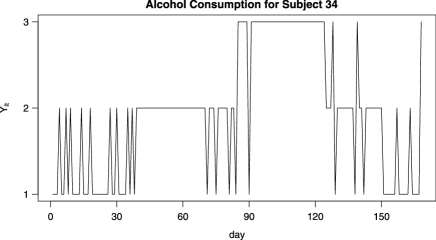
Figure 1: The time series plot of alcohol consumption for Subject 34. The vertical axis has tickmarks at 1 (0 drinks), 2 (1–4 drinks) and 3 (5 or more drinks).

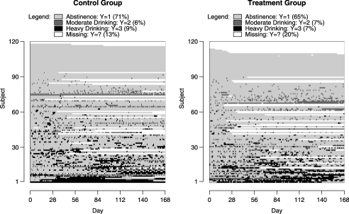
Figure 2: A representation of the observed alcohol consumption time series for all $N=240$ subjects in the clinical trial. They are approximately sorted from top to bottom (within their treatment group) in order of increasing alcohol consumption.

We include 4 covariates in the models we fit:

1. Treatment. Half the subjects were randomly assigned to receive the drug Naltrexone, and the other half were assigned a placebo.

2. Sex. There were 175 men in the study, and 65 women.

3. Previous drinking behavior. Each study participant was asked to estimate the proportion of days prior to the study during which they drank, and during which they drank heavily. We used these two variables, denoted $D_{(i,\mathrm{drink})}$ and $D_{(i,\mathrm{heavy})}$, to calculate the proportion of days prior to the trial during which each subject drank moderately, denoted $D_{(i,\mathrm{moderate})}=D_{(i,\mathrm{drink})}-D_{(i,\mathrm{heavy})}$, and then created a “previous drinking behavior” index, $Z_{i}=D_{(i,\mathrm{moderate})}+2D_{(i,\mathrm{heavy})}\in[0,2]$. This variable is a univariate summary of a subject’s previous drinking behavior which is approximately unimodal.

4. Time. We measure time in days from $1,2,\ldots,T=168$. Subjects did not necessarily participate during the same stretch of actual calendar days, so this variable is only a measure of the relative time within the clinical trial.

Prior to fitting the models, we scale these 4 input variables to have a mean of zero and a standard deviation of $1/2$, so that the regression coefficients are comparable on the same scale. The ordinal drink counts and covariates for all 240 subjects are available as supplementary material in Shirley et al. (2009).

2.2 Existing models

Current models for alcohol data range from relatively simple models that compare univariate summary statistics among different treatment groups to more complex failure time models, linear mixed models and latent transition models. Wang et al. (2002) provide a good review and a discussion of why very simple summary statistics are not adequate for modeling drinking outcomes over time. Some examples of such summary statistics are average number of drinks per day and percentage of days abstinent. Average drinks per day, for example, might not differentiate between one subject who drinks moderately every day of the week and another subject who abstains from drinking during the week, and then binges on the weekend. Percentage of days abstinent, on the other hand, does not differentiate between light and heavy drinking, and does not provide information about the pattern of abstinence across time.

Wang et al. suggest the use of multivariate failure time models for alcohol data. These models can be used to predict the amount of time before the next relapse. One shortcoming of such models is that they require a strict definition of a relapse in order to define an “event.” Although alcohol researchers agree on a conceptual definition of a relapse as a failure to maintain desired behavior change, they do not agree on an operational definition of relapse [Maisto et al. (2003)]. For example, do two days of heavy drinking separated by a single day of abstinence constitute two relapses or just one? Does one isolated day of heavy drinking constitute a relapse or just a “lapse”? Any inference drawn from a multivariate failure time model is conditional on the definition of a relapse. Maisto et al. (2003) show that the choice of relapse definition makes a meaningful difference in estimates of relapse rates and time to first relapse.

McKay et al. (2006) review GEE models for repeated measures alcohol data. Although GEE models are useful in many ways, they are best suited to estimate the population mean of drinking given a set of covariates, rather than to make predictions for an individual given the individual’s covariates and drinking history. Latent transition models, which are closely connected to HMMs, have been proposed in the literature on addictive behavior [e.g., Velicer, Martin and Collins (1996)]. These models typically require a multivariate response vector at each time point, and are fit for data with a small number of time points, whereas our data have a univariate response at each time point and a long time series for each subject.

Mixed effects models are in principle well suited to making individual predictions [McKay et al. (2006)], but a rich structure for the serial correlation must be considered to accommodate the flat stretches and bursts nature of alcohol data, something which has not been considered thus far in the alcohol research literature. This paper introduces two such models—a mixed effects HMM and a mixed effects Markov model for alcohol data.

2.3 Motivation for a Markov model or HMM

One of the important goals of this research is to fit a model to alcohol data that can provide a rich description of the changes in a subject’s drinking behavior through time. A first-order Markov (chain) model is a suitable starting point in the search for such a model. It models the observed data at a high resolution—daily observations—as opposed to some lower-dimensional summary statistic of the data, such as the time until the first relapse. By modeling the observations themselves, we can infer the distribution of any lower-dimensional summary statistic we wish after fitting the model. The serial dependence structure of a Markov model, however, is such that it may not be suitable for data that exhibit long-term dependence.

The HMM is an attractive alternative to the first-order Markov model because its serial dependence structure allows for longer-term dependence. As we have stated previously, drinking behavior among individuals following their AUD treatment is erratic, commonly exhibiting flat stretches and bursts, creating long-term dependence. Longitudinal data of this form suggest that a parameter-driven model might fit the data better than an observation-driven model. Cox (1981) originally coined the term parameter-driven for models in which an underlying, potentially changing “parameter process” determines the distribution of observed outcomes through time, such that the observed outcomes depend on each other only through the underlying parameter process. Observation-driven models, on the other hand, model observed outcomes directly as functions of previously observed outcomes. State-space models and HMM’s (which are a subset of state-space models) are widely used examples of parameter-driven models.

A second, very important motivation for the HMM for alcohol data is its potential clinical interpretation: it is a quantitative model that closely corresponds to a well-developed theoretical model of relapse known as the cognitive-behavioral model of relapse. This theory suggests that the cause of an alcohol relapse is two-fold: First, the subject must be in a mental and/or physical condition that makes him or her vulnerable to engaging in an undesired level of drinking. In other words, if the subject were given an opportunity to drink alcohol, he or she would be unable to mount an effective coping response, that is, a way to avoid drinking above some desired level (usually abstinence or a moderate level of drinking). A subject’s ability to cope can depend on time-varying cognitive factors, such as expectations of the results of drinking, time-varying noncognitive factors, such as level of stress, desire to drink and social support, and background variables such as age or sex. The second condition that must be present for a relapse is that the subject encounters a high-risk drinking situation, which is a setting associated with prior heavy alcohol use. Common examples are a negative mood, interpersonal problem(s) and an invitation to drink. McKay et al. (2006) and Marlatt and Gordon (1985) contain more detailed discussions of the traditional cognitive-behavioral model of relapse, and Witkiewitz and Marlatt (2004) update Marlatt and Gordon (1985).

The HMM connects to the cognitive-behavioral model of relapse in the following way: The hidden states in the HMM correspond to the vulnerability of the subject to drinking if faced with a high risk situation, and the number of drinks consumed on a given day is affected by the subject’s vulnerability to drinking on the given day (the hidden state) and whether the subject faced a high-risk drinking situation on that day. The conditional distributions of the observations given the hidden states model the prevalence of high-risk drinking situations for each hidden state. Interpreting the HMM this way suggests that relapse is not necessarily an observable state—it is a hidden state that presumably leads to heavy drinking with higher probability than other states, but not with certainty. Via this correspondence to the cognitive-behavioral model of relapse, the HMM has potential to make an important contribution to the alcohol literature in its ability to provide quantitative insight into a popular qualitative model for relapse.

3 The models

The data we wish to model consist of categorical observations $Y_{it}\in(1,2,\ldots,M)$, for subjects $i=1,\ldots,N$, and time points $t=1,\ldots,n_{i}$ (where $n_{i}=168$ for all subjects in our data set). We also observe the $p\times 1$ covariate vectors $\mathbf{X}_{it}=(X_{it1},X_{it2},\ldots,X_{itp})^{\prime}$ for each subject at each time point. We consider two types of models in this paper: (1) a hidden Markov model, and (2) a Markov model.

3.1 Hidden Markov model

The HMM we fit consists of a mixed effects multinomial logit model for each row of the hidden state transition matrix, and multinomial models for (1) the conditional distributions of the observations given the hidden states, hereafter called the conditional distributions of the HMM, and (2) the initial hidden state distribution. The model includes an unobserved, discrete hidden state, $H_{it}\in(1,2,\ldots,S)$ for each individual $i$ at each time point $t$, and we denote an HMM with $S$ hidden states as an HMM($S$).

The hidden state transition matrix is an $S\times S$ matrix, in which each row has probabilities that are modeled using a mixed effects multinomial logit model:

$$p\bigl{(}H_{(i,t+1)}=s|H_{it}=r,\mathbf{X}_{it},\bolds{\alpha}_{ir},\bolds{\beta}_{r}\bigr{)}=\frac{\exp(\alpha_{irs}+\mathbf{X}_{it}^{\prime}\bolds{\beta}_{rs})}{1+\sum_{k=2}^{S}\exp(\alpha_{irk}+\mathbf{X}_{it}^{\prime}\bolds{\beta}_{rk})}$$ (1)

for $r=1,\ldots,S$, $s=2,\ldots,S$, $i=1,\ldots,N$, and $t=1,\ldots,T-1$. For $s=1$, the numerator is set equal to 1, making the first category the baseline category. The random intercepts are modeled using normal distributions, where $\alpha_{irs}\sim N(\mu_{rs},\sigma_{rs}^{2}),$ for $i=1,\ldots,N$, $r=1,\ldots,S$, and $s=2,\ldots,S$.

The inclusion of $S(S-1)$ random intercepts for each subject means that each subject’s transition matrix is fully flexible to reproduce every possible set of cell frequencies for that subject. The regression effects, on the other hand, are “fixed” effects that are constant across all subjects. They may, however, be time-varying.

The conditional distributions of the HMM are multinomial distributions, where

$$p(Y_{it}=m|H_{it}=s,\mathbf{p}_{s})=p_{sm}$$ (2)

for $m=1,\ldots,M$ and $s=1,\ldots,S$, where $\mathbf{p}_{s}=(p_{s1},p_{s2},\ldots,p_{sM})$ is a vector of multinomial probabilities, for $s=1,\ldots,S$. Last, the initial hidden state distribution for the HMM is a multinomial distribution with probability vector $\bolds{\pi}=(\pi_{1},\ldots,\pi_{S})$. For the hidden Markov model, the collection of all parameters is $\bolds{\theta}=(\bolds{\alpha},\bolds{\beta},\bolds{\mu},\bolds{\sigma},\bolds{\pi},\mathbf{P})$.

3.2 Markov model

The other model we consider is a first-order Markov model, in which the set of probabilities in each row of the transition matrix is defined according to the same model described in Section 3.1, a mixed effects multinomial logit model. The outcome for individual $i$ at time $t+1$, $Y_{(i,t+1)}$, depends on the previous observation for that individual, $Y_{it}$, in the following way:

$$p\bigl{(}Y_{(i,t+1)}=m|Y_{it}=j,\mathbf{X}_{it},\bolds{\alpha}_{ij},\bolds{\beta}_{j}\bigr{)}=\frac{\exp(\alpha_{ijm}+\mathbf{X}_{it}^{\prime}\bolds{\beta}_{jm})}{1+\sum_{k=2}^{M}\exp(\alpha_{ijk}+\mathbf{X}_{it}^{\prime}\bolds{\beta}_{jk})}$$ (3)

for $j=1,\ldots,M$, $m=2,\ldots,M$, $i=1,\ldots,N$, and $t=1,\ldots,T-1$. As before, for $m=1$, the numerator equals 1. The random intercepts are given normal distributions, where $\alpha_{ijm}\sim N(\mu_{jm},\sigma_{jm}^{2}),$ for $i=1,\ldots,N$, $j=1,\ldots,M$, and $m=2,\ldots,M$.

The initial values, $Y_{i1}$, for $i=1,\ldots,N$, are modeled as i.i.d. draws from a multinomial distribution with probability vector $\bolds{\pi}=(\pi_{1},\ldots,\pi_{M})$. For the Markov model, the collection of all parameters is $\bolds{\theta}=(\bolds{\alpha},\bolds{\beta},\bolds{\mu},\bolds{\sigma},\bolds{\pi})$.

3.3 Missing data

Following Oslin et al. (2008)’s analysis of the trial we are considering, we will assume that the missing data is missing at random, that is, the missingness mechanism is independent of the missing data given the observed data and covariates. For the HMM, we make the additional assumption that the missingness mechanism is independent of the hidden states given the observed data and covariates, in order to do inference on the hidden states as well as the model parameters [Gelman et al. (2004), Chapter 21]. A sensitivity analysis for this assumption is a valuable topic for future research, but outside the scope of this paper. There is a considerable literature on missing data in longitudinal addiction studies, including Albert (2000, 2002) and Longford et al. (2000), which might guide one’s choices regarding the design of a sensitivity analysis.

3.4 Discussion of models

The first-order Markov model is nested within an HMM with $M$ or more hidden states. Also, an HMM with $S$ hidden states is nested within an HMM with more than $S$ hidden states. An HMM is a mixture model, whose mixing distribution is a first-order Markov chain. It has been applied to problems in numerous fields [for lists of examples, see MacDonald and Zucchini (1997), Scott (2002) or Cappe, Moulines and Ryden (2005)], but not previously to alcohol consumption time series data.

4 Model fits and comparison

4.1 Model fits

We fit the HMM(3) and the Markov model usingMetropolis-within-Gibbs MCMC algorithms whose details are described in the Appendix. We ran three chains for each model and discarded the first 10,000 iterations of each chain as burn-in. We used the next 10,000 iterations as our posterior sample and assessed convergence using the potential scale reduction factor [Gelman et al. (2004)], and found that $\hat{R}<1.02$ for all parameters in the models. Visual inspection of trace plots provide further evidence that the posterior samples converged to their stationary distributions. The autocorrelation of the posterior samples of $\bolds{\beta}$ were the highest of all the parameters, such that total effective sample size from three chains of 10,000 iterations each was between 200 and 300. The transition probabilities for each subject and time point, on the other hand, had much lower autocorrelations, such that for a given transition probability, three chains of 10,000 iterations each yielded a total effective sample size of about 5000 approximately independent posterior samples. Since transition probabilities are the most important quantity of interest in our analysis, the Monte Carlo error associated with our estimated treatment effects is small.

All the parameters were given noninformative or weakly informative priors, which are described in the Appendix. The algorithm for both models consisted of sampling some of the parameters using univariate random-walk Metropolis steps, and others from their full conditional distributions. When fitting the Markov model, if a subject’s data were missing for $t_{\mathrm{mis}}$ steps, we computed the $(t_{\mathrm{mis}}+1)$-step transition probability to calculate the likelihood of the current parameters given the data, and alternated between sampling $\mathbf{Y}_{\mathrm{mis}}\sim p(\mathbf{Y}_{\mathrm{mis}}|\mathbf{Y}_{\mathrm{obs}},\mathbf{X},\bolds{\theta})$ and $\bolds{\theta}\sim p(\bolds{\theta}|\mathbf{Y}_{\mathrm{obs}},\mathbf{Y}_{\mathrm{mis}},\mathbf{X})$. Likewise for the HMM, we alternated sampling $\mathbf{H}\sim p(\mathbf{H}|\mathbf{Y}_{\mathrm{obs}},\mathbf{X},\bolds{\theta})$ and $\bolds{\theta}\sim p(\bolds{\theta}|\mathbf{Y}_{\mathrm{obs}},\mathbf{H},\mathbf{X})$. We sampled $\mathbf{H}$ using a forward-backward recursion as described in Scott (2002), substituting $(t_{\mathrm{mis}}+1)$-step transition probabilities between hidden states when there was a string of $t_{\mathrm{mis}}$ missing observations for a given subject.

The hidden states of an HMM have no a priori ordering or interpretation, and as a result, their labels can “switch” during the process of fitting the model from one iteration of the MCMC algorithm to the next, without affecting the likelihood [Scott (2002)]. We experienced label switching when the starting points for the MCMC algorithm were extremely widely dispersed, but when we used more narrowly dispersed starting points, each chain converged to the same mode of the $S!$ symmetric modes of the posterior distribution. We discuss our procedure for selecting starting points for the parameters in the MCMC algorithms in the Appendix.

4.2 Model comparison

We present the DIC of the two models in this section, but we ultimately don’t rely on it as a formal model selection criterion. Instead we use posterior predictive checks to compare the two models, and combine this analysis with existing scientific background knowledge to motivate our model choice, which suggests that the HMM(3) is more promising.

The Markov model converged to a slightly lower mean deviance than the HMM(3), where the deviance is defined as $D(\mathbf{Y},\bolds{\theta})=-2\log{p(\mathbf{Y}|\bolds{\theta})}$. Table 1 contains a summary of the deviance for both models, where $\bar{D}(\mathbf{Y},\bolds{\theta})$ is the mean deviance across posterior samples of $\bolds{\theta}$, and $D(\mathbf{Y},\bar{\bolds{\theta}})$ is the deviance evaluated at the posterior mean, $\bar{\bolds{\theta}}$. For the Markov model, deviance calculations were done using the parameter vector $\bolds{\theta}=(\bolds{\alpha},\bolds{\beta},\bolds{\pi})$, whereas for the HMM(3), the parameter vector $\bolds{\theta}=(\bolds{\alpha},\bolds{\beta},\bolds{\pi},\mathbf{P})$. That is, for both models, we compute the probability of the data given the parameters in the likelihood equation, and don’t factor in the prior probabilities of the random effects, $p(\bolds{\alpha}|\bolds{\mu},\bolds{\sigma})$. The Markov model has a higher estimated effective number of parameters, $pD$, and also has a higher DIC, which is an estimate of a model’s out of sample prediction error [Spiegelhalter et al. (2002)]. The estimates of $pD$ and DIC had low Monte Carlo estimation error (approximately ${\pm}$5), as estimated by recomputing them every 1000 iterations after burn-in.

Table 1: Summary of the DIC of the models

Model	$\bolds{\bar{D}(\mathbf{Y},\bolds{\theta})}$	$\bolds{D(\mathbf{Y},\bar{\bolds{\theta}})}$	$\bolds{pD}$	DIC
Markov	19,871	19,183	688	20,560
HMM(3)	19,902	19,303	599	20,500

Model selection criteria such as BIC and DIC, however, are well known to be problematic for complicated hierarchical models, mixture models such as an HMM and models with parameters that have non-normal posterior distributions [Spiegelhalter et al. (2002), Scott (2002)]. For this reason, we choose not to select a model [between the Markov model and the HMM(3)] based on formal criteria such as these. Instead, we examine the fit of each model using posterior predictive checks and highlight each of their advantages and disadvantages. We ultimately focus most of our attention on the HMM(3) because of its potential for clinical interpretability in terms of the cognitive behavioral model of relapse (Section 2.3), which suggests that a relapse is not equivalent to a heavy drinking episode, but rather, it may be better modeled as an unobserved state of health.

5 Interpreting the model fits

We begin by looking at the parameter estimates of the Markov model and HMM(3).

5.1 Conditional distributions of the HMM

The hidden states of the HMM(3) can be characterized by their conditional distributions, which are multinomial distributions with three cell probabilities, $p_{sm}=p(Y_{it}=m|H_{it}=s)$ for outcomes $m=1,2,3$ and hidden states $s=1,2,3$. The posterior distributions of $p_{sm}$ are summarized in Table 2. Each conditional distribution puts most of its mass on a single outcome, and we therefore label the hidden states according to which outcome has the largest probability under their associated conditional distributions: The first hidden state is labeled “Abstinence” (“A”), the second hidden state is labeled “Moderate Drinking” (“M”), and the third hidden state is labeled “Heavy Drinking” (“H”). The Moderate and Heavy Drinking states each leave a small, but significant (as indicated by their 95% posterior intervals excluding zero) probability of a different outcome from moderate ($Y=2$) and heavy ($Y=3$) drinking, respectively.

Table 2: Conditional Distributions of the HMM(3)

	Posterior mean	Posterior stand. errors	State label
$\hat{\mathbf{p}}_{1}$	(0.997, 0.003, 0.000)	(0.001, 0.001, 0.000)	“Abstinence”
$\hat{\mathbf{p}}_{2}$	(0.026, 0.956, 0.018)	(0.012, 0.012, 0.005)	“Moderate Drinking”
$\hat{\mathbf{p}}_{3}$	(0.031, 0.004, 0.966)	(0.006, 0.002, 0.007)	“Heavy Drinking”

5.2 Transition probabilities

The posterior distributions of the parameters associated with the transition matrices for the Markov model and the HMM(3) are similar. This is not surprising, considering that if $p_{11}=p_{22}=p_{33}=1$, then the HMM(3) is equivalent to the Markov model, and from Table 2 we see that the estimates of $p_{11},p_{22}$ and $p_{33}$ are almost equal to 1. We will not discuss the posterior distributions of these parameter estimates here, though, because the form of the multinomial logit model for each row of the transition matrices makes them somewhat difficult to interpret. Instead, we present the estimated mean transition matrices for both models:

$$\hskip 12.0pt\hat{Q}_{\mathrm{Markov}}=\pmatrix{0.97&0.02&0.01\vspace*{2pt}\cr 0.75&0.21&0.04\vspace*{2pt}\cr 0.45&0.03&0.52},\qquad\hat{Q}_{\mathrm{HMM(3)}}=\pmatrix{0.98&0.01&0.01\vspace*{2pt}\cr 0.72&0.26&0.02\vspace*{2pt}\cr 0.41&0.02&0.57}.$$ (4)

These are the posterior mean transition matrices for the Markov model and HMM(3) for a subject with average random intercepts, and the average value for each covariate: $\mathbf{X}_{i}=(0,0,0,0)^{\prime}$. Formally,

$$\hat{Q}_{\mathrm{Model}}(j,m)=\frac{1}{G}\sum_{g=1}^{G}\biggl{(}\frac{\exp{(\mu_{jm}^{(g)})}}{1+\exp{(\mu_{j2}^{(g)})}+\exp{(\mu_{j3}^{(g)})}}\biggr{)}$$

for $j=1,\ldots,3$, $m=2,3$, and posterior samples $g=1,\ldots,G$, where for $m=1$, the numerator is replaced by the value 1. Setting the time variable equal to zero corresponds to calculating the mean transition matrix on day 84 of the 168-day clinical trial. Note that Sex and Treatment are binary variables, which means that no individual subject has the exact design matrix used to calculate the transition probabilities in Equation (4). Later in Section 6 we will more carefully analyze the transition matrices bearing this in mind, but for now we are only interested in rough estimates of the transition probabilities.

The estimates of the mean transition probabilities are very similar between the two models. One interesting feature is that, on average, for both models, the most persistent state is Abstinence, the second most persistent state is Heavy Drinking, and the least persistent state is Moderate Drinking. The Moderate Drinking and Heavy Drinking states don’t communicate with each other with high probability under either model (for a person with average covariates). We fully analyze the covariate effects on the transition matrix in Section 6.

5.3 Initial state probabilities

The posterior distributions of the initial state probability vectors for the two models were nearly identical, where their posterior means were $\hat{\bolds{\pi}}=(93.6\%,3.4\%,3.0\%)$ for both models, and the posterior standard deviation was about 1.5% for all three elements of $\bolds{\pi}$ (for both models).

6 The treatment effect

To estimate the effects of covariates, including the treatment variable, on the transition probabilities of the hidden state transition matrix for the HMM(3) (where a similar analysis could be done for the Markov model if desired), we perform average predictive comparisons as described in Gelman and Hill (2007), pages 466–473. The goal is to compare the value of some quantity of interest, such as a transition probability, calculated at two different values of an input variable of interest, such as Treatment, while controlling for the effects of the other input variables. Simply setting the values of the other inputs to their averages is one way to control for their effects, but doing so can be problematic when the averages of the other inputs are not representative of their distributions, as is the case for binary inputs, for example. An average predictive comparison avoids this problem by calculating the quantity of interest at two different values of the input of interest while holding the other inputs at their observed values, and averaging the difference of the two quantities across all the observations.

In the context of the HMM(3), if we denote the input variable of interest by $U$, and consider high and low values of this variable, $u^{\mathrm{(hi)}}$ and $u^{\mathrm{(lo)}}$, and denote the other input variables for individual $i$ at time $t$ by $\mathbf{V}_{it}$, then we can compute the average difference in transition probabilities calculated at the two values of $U$ as follows:

$$B_{jm}(U) = \frac{1}{N(T-1)}$$

$${}\times\sum_{i=1}^{N}\sum_{t=1}^{T-1}\bigl{[}\mathrm{P}\bigl{(}H_{(i,t+1)}=m|H_{it}=j,\bolds{\theta},u_{it}=u^{\mathrm{(hi)}},\mathbf{v}_{it}\bigr{)}$$

$$\hskip 47.0pt{}-\mathrm{P}\bigl{(}H_{(i,t+1)}=m|H_{it}=j,\bolds{\theta},u_{it}=u^{\mathrm{(lo)}},\mathbf{v}_{it}\bigr{)}\bigr{]}$$

for $j,m=1,\ldots,3$. We call $B_{jm}(U)$ the average transition probability difference for input variable $U$ for transitions from hidden state $j$ to hidden state $m$.

Figure 3 displays 95% posterior intervals for the average transition probability differences for all four covariates that are incorporated into the transition matrix of the HMM(3), for all $3^{2}=9$ possible transitions. The treatment, Naltrexone, appears to have a moderate negative effect on the probabilities of a transition from Heavy-to-Heavy and Abstinent-to-Heavy, as is evidenced by the fact that the 95% posterior intervals for these average transition probability differences lie mostly below zero [the intervals are $(-19.9\%,2.5\%)$ and $(-4.1\%,1.1\%)$, respectively]. Heavy-to-Heavy transitions occur, on average, about 9% less often for those using Naltrexone, and Abstinent-to-Heavy transitions occur, on average, about 1.5% less often for those using Naltrexone. This is a desired outcome: These intervals indicate that Naltrexone may be effective in improving certain aspects of drinking behavior, because a reduction in these transition probabilities would most likely result in a decrease in heavy drinking, according to the estimated conditional distributions associated with these hidden states. Conversely, Naltrexone appears to have a significant positive effect on the probability of a transition from Moderate-to-Heavy, occurring about 3.5% more often on average for Naltrexone-takers, which, on average,would lead to increased heavy drinking.

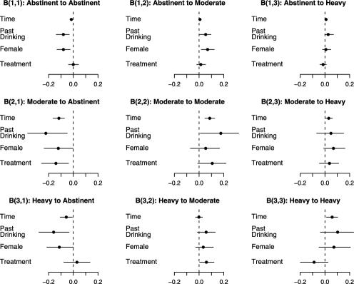
Figure 3: 95% posterior intervals of the average transition probability differences for each of the four input variables and for each of the nine transition probabilities in the HMM(3). For the binary input variables Treatment and Sex, we set the high values, $u^{\mathrm{(hi)}}$, as Naltrexone and Female, and the low values, $u^{\mathrm{(lo)}}$, as Control and Male, respectively, and for the continuous input variables, Past Drinking and Time, we set the high and low values to the mean $\pm$ 1 sd of their respective distributions.

Other covariate effects visible in Figure 3 include the following:

• All else being equal, women are more likely than men to make transitions into the Moderate and Heavy states.

• Drinking heavily in the past is associated with higher transition probabilities into the Moderate and Heavy states.

• Transitions into the Moderate and Heavy states are more likely to occur later in the clinical trial than earlier in the clinical trial.

• The 95% intervals for the average transition probability differences are noticeably shorter for transitions out of the Abstinence state, because that is where subjects are estimated to spend the most time, and with more data comes more precise estimates.

6.1 Covariate effects on the stationary distribution

To further summarize the effects of the covariates on drinking behavior, we can compute average stationary probability differences instead of average transition probability differences. This provides a slightly more interpretable assessment of the treatment effect on drinking behavior because the stationary distribution contains a clinically important summary statistic: the expected percentages of time a subject will spend in each hidden state, given that the HMM is stationary. An effective treatment would reduce the expected amount of time spent in the Heavy Drinking state.

The model we fit is a nonhomogenous (i.e., nonstationary) HMM, so, by definition, it does not have a stationary distribution. We would still, however, like to make inferences about a subject’s long-term behavior conditional on whether or not he or she took Naltrexone. One strategy for estimating how much time will be spent in each state is through posterior predictive simulations of the hidden states themselves. Another strategy, which we discuss here, is to compute the stationary distribution of the hidden state transition matrix on the last day of the trial for all subjects. This can be interpreted as a way of projecting drinking behavior into the long-term future without extrapolating the effect of time beyond the clinical trial, by assuming that each subject has reached a stationary pattern of behavior at the end of the trial. Figure 4 contains 95% posterior intervals of the average stationary probability differences for the covariates Treatment, Sex and Past Drinking, where the HMM(3) is assumed to be stationary beginning on the last day of the trial.

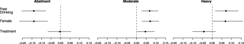
Figure 4: 95% posterior intervals of average stationary probability differences for the three covariates (other than time) incorporated into the HMM(3) transition matrix.

On average, the use of Naltrexone appears to decrease the amount of time spent in the Heavy drinking state by about 5%, and increase the amount of time spent in the Moderate drinking state by the same amount. Women and subjects who drank heavily prior to the trial also are predicted to spend more time in the Heavy drinking state in the long run. These estimates are consistent with the average transition probability differences displayed in Figure 3, and provide a slightly more concise summary of the covariate effects.

6.2 Heterogeneity among individuals

Another important aspect of the model fit is the degree of heterogeneity that is present among individuals, which is modeled by the random intercepts as well as the covariate effects embedded in the HMM(3) hidden state transition matrix. To explore this, we calculate the posterior mean of each of the $3^{2}=9$ transition probabilities for each subject $i$ at a given time point $t$,

$$\hat{Q}_{it}(r,s)=\frac{1}{G}\sum_{g=1}^{G}\mathrm{P}\bigl{(}H_{(i,t+1)}=s|H_{it}=r,X_{it},\bolds{\alpha}^{(g)},\bolds{\beta}^{(g)},\bolds{\pi}^{(g)}\bigr{)}$$ (6)

for $i=1,\ldots,N$, $t=84$ (the midpoint of the trial), $r,s=1,2,3$, and posterior samples $g=1,\ldots,G$. In Figure 5 we plot density estimates of each of the $3^{2}=9$ sets of $N$ transition probability posterior means (measured at time $t=84$).

Figure 5: Density estimates of the $3^{2}=9$ sets of posterior mean transition probabilities in the HMM(3), where the posterior means are calculated for each individual at the midpoint of the trial ($t=84$), and each of the 9 the transition probability densities are therefore estimated using $N=240$ data points.

The density estimates of these posterior mean transition probabilities represent heterogeneity among individuals from two sources: the random intercepts and the covariate effects. By comparing Figure 3 to Figure 5, it is clear that the differences in mean transition probabilities among individuals are larger than the differences implied by covariate effects alone. The largest average transition probability differences, illustrated in Figure 3, were approximately ${\pm}$0.2, and were due to differences in the subjects’ previous drinking behavior. We see from Figure 5, however, that the differences between transition probabilities across individuals is often greater than 0.5, and can be as large as 1, such that a particular transition is certain for one individual, and has zero probability for another individual. Specifically, transition probabilities are relatively similar across subjects when the subjects are in the Abstinent state, but are highly variable across subjects when the subjects are in the Moderate and Heavy states. If a subject is in the Abstinent state, their probability of remaining in the Abstinent state for an additional day is above 80% for most subjects, regardless of the values of his or her observed covariates and random intercepts (which represent the effects of unobserved covariates). On the other hand, if a subject is in the Moderate or Heavy state, his or her next transition is highly uncertain: depending on the individual, he or she may have a very high or a very low probability of remaining in the same state for another day. The fact that the random intercepts are explaining more variation in the estimated transition probabilities than any individual covariate suggests that it might be useful for future studies to record as many additional covariates as possible. Such a design might reduce the amount of unexplained heterogeneity across individuals that must be accounted for by the random intercepts. This result also highlights the need for random effects in this particular model, as well as the need for studying the inclusion of random effects into HMMs in general, as they can have a profound effect on the fit of the model.

7 Goodness of fit of the models

In this section we use posterior predictive checks to examine the fit of the HMM(3) and the difference between the HMM(3) and the Markov model.

7.1 Mean and variance of drinking days across subjects

As a first check of the goodness of fit of our model, we performed posterior predictive checks [Gelman et al. (2004)] of the mean and variance of the number of moderate and heavy drinking days across all subjects (a total of four statistics of interest). The specific steps we took are as follows: For each of these four statistics, we computed its observed value from the data, and denoted this $t(\mathbf{Y}^{\mathrm{obs}})$. Then, for posterior samples $g=1,\ldots,G$, we

1. simulated $\bolds{\alpha}^{\mathrm{rep}}|\bolds{\mu}^{(g)},\bolds{\sigma}^{(g)}$, where $\bolds{\alpha}^{\mathrm{rep}}$ is a set of random effects to represent a new set of subjects from the population,

2. simulated $\mathbf{H}^{\mathrm{rep}}|\bolds{\alpha}^{\mathrm{rep}},\bolds{\beta}^{(g)},\bolds{\pi}^{(g)},\mathbf{X}$,

3. simulated $\mathbf{Y}^{\mathrm{rep}}|\mathbf{H}^{\mathrm{rep}},\mathbf{P}^{(g)}$, and

4. computed $t(\mathbf{Y}^{\mathrm{rep}})$,

where the parameters superscripted by $(g)$ are taken from the posterior samples obtained from the MCMC algorithm. By simulating new random effects, $\bolds{\alpha}^{\mathrm{rep}}$, we are checking to see that the model adequately captures heterogeneity across subjects. We compared the values of $t(\mathbf{Y}^{\mathrm{obs}})$ to the distributions of $t(\mathbf{Y}^{\mathrm{rep}})$ for the four statistics of interest, and found no evidence of a lack of fit; that is, the observed values of $t(\mathbf{Y}^{\mathrm{obs}})$ were not located in the extreme tails of the distributions of $t(\mathbf{Y}^{\mathrm{rep}})$. Table 3 contains summaries of these posterior predictive checks.

Table 3: Summaries of the posterior predictive checks of the mean and variance of moderate and heavy drinking days. $s^{2}_{\mathrm{mod}}$ and $s^{2}_{\mathrm{heavy}}$ are the variances of the number of moderate and heavy drinking days across subjects, respectively, and $\bar{x}_{\mathrm{mod}}$ and $\bar{x}_{\mathrm{heavy}}$ are the means of the number of moderate and heavy drinking days across subjects, respectively. The middle 5 columns contain the 2.5th, 25th, 50th, 75th and 97.5th quantiles of the distributions of $t(\mathbf{Y}^{\mathrm{rep}})$, and the rightmost column contains the observed values $t(\mathbf{Y}^{\mathrm{obs}})$, and the proportion of the simulated statistics that were less than these values

Statistic	2.5%	25%	50%	75%	97.5%	Observed (quantile)
$s^{2}_{\mathrm{mod}}$	335.9	393.5	430.6	477.6	554.6	524.8 (0.92)
$s^{2}_{\mathrm{heavy}}$	400.6	502.9	558.4	608.4	722.7	618.5 (0.78)
$\bar{x}_{\mathrm{mod}}$	009.8	010.5	010.9	011.3	012.1	011.3 (0.73)
$\bar{x}_{\mathrm{heavy}}$	011.6	012.7	013.4	013.9	015.1	013.7 (0.65)

7.2 First drinking day

Another common quantity of interest in alcohol research is the time until a subject’s first drink, also known as the first drinking day, or FDD. This variable is often treated as the primary outcome in clinical trials for AUD treatments. We performed a posterior predictive check of the mean and variance of this statistic across subjects using the same steps as are outlined in Section 7.1. This check relates not only to the heterogeneity of behavior across subjects, but also to the patterns of drinking behavior across time.

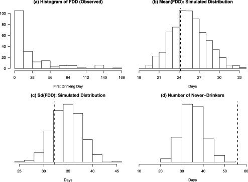
Figure 6: (a) The histogram of observed FDD; (b) the histogram of simulated values of the mean FDD across subjects; (c) the histogram of simulated values of the standard deviation of FDD across subjects; (d) the histogram of the simulated distribution of Never-Drinkers. In each case, the values calculated from the simulated distributions were computed by ignoring the days that were missing for each subject, so that the simulated values are directly comparable to the observed values, denoted by the vertical dotted lines in each figure.

Figure 6 contains plots summarizing the posterior predictive checks of FDD. Figure 6(a) contains a histogram of the observed values of FDD for all subjects; the empirical distribution is skewed to the right, and contains only 184 points, because 56 subjects exhibit a combination of missing data or abstinence throughout the whole trial. Figures 6(b) and 6(c) contain histograms of the simulated distributions of the mean and standard deviation of FDD across subjects, for the subset of subjects who drank at least once, with dotted lines representing the observed values. The observed values lie within the center parts of their simulated distributions, indicating an adequate fit. Last, Figure 6(d) contains a histogram of the simulated values of the number of “Never-Drinkers” among the 240 subjects, that is, those who never drink throughout the course of the clinical trial, via a combination of abstinence and missing data. The observed number of Never-Drinkers is 56 (out of 240), but in general, the model reproduces data sets in which there are about 20–50 Never-Drinkers. This indicates a slight lack of fit—there appears to be a set of individuals among the subjects (who never drink) whose behavior is not well captured by the model. A similar lack of fit in other settings has been remedied by the use of a mover-stayer model [Albert (1999), Cook, Kalbfleisch and Yi (2002)], in which a latent class of subjects is constrained to exhibit constant behavior over the whole time series, and membership in this class is estimated from the data. On the other hand, it may be clinically justifiable to suggest that a subject always has a nonzero probability of drinking, even if in a given sample of days he or she never drinks. In the fit of the HMM(3), the prior distributions on the random effects means ($\bolds{\mu}$) virtually prevent any subject from having a transition probability of zero by design. Transition probabilities can be very small, but never zero.

7.3 Patterns across time

Further posterior predictive checks demonstrate that the HMM(3) is able to model nonlinear, nonstationary and heteroscedastic drinking behavior. To see this, we divided the trial period of 24 weeks into 6 blocks of 4-week time periods, and performed posterior predictive checks on the mean and variance of abstinent, moderate and heavy drinking days within each time period. In other words, we recreated the four posterior predictive checks illustrated in Table 3 for data in each of six time periods, and extended the analysis to include the mean and standard deviation of abstinent days across subjects for each time period.

Figure 7 contains a visual summary of all 36 of these posterior predictive checks, where the $x$-axis in each of the six plots is time. The boxplots in each of the six plots display the distributions of the simulated values of the given statistics during each time period, and the black lines display the observed values of these statistics. The plot in the upper left corner, for example, shows that the observed mean of abstinent days (across subjects) decreased over the course of the clinical trial, from about 23 days out of a possible 28 days in the first 4-week time period to about 18 out of 28 days in the last 4-week time period, and that this decreasing trend is nonlinear. The HMM(3) captures this nonlinear trend, with a slight underestimate of the mean number of abstinent days toward the end of the trial (in the last 4–8 weeks). Furthermore, the lower left-hand plot shows that the standard deviation of the number of days of abstinence (across subjects) increases as the trial progresses, also in a nonlinear way. The HMM(3) adequately models this heteroscedasticity, with only a slight underestimate of the standard deviation of abstinent days in the last 8–12 weeks. Regarding moderate and heavy drinking, the model appears to adequately describe both the mean and standard deviation of moderate drinking days for each time period, but fails to fully capture the apparent quadratic trend in the mean and standard deviation of heavy drinking through time (both of these quantities appear to increase from the beginning of the trial until the middle of the trial, and then decrease until the end of the trial). The observed values of these statistics, though, never fall outside of the tails of the simulated distributions, indicating no major lack of fit. These posterior predictive checks illustrate the flexibility of the HMM as it is formulated in Section 3.1. Note that for categorical outcomes, the mean and sd are determined by the same sets of parameters, and that the observed percentages of each categorical outcome are negatively correlated by definition (because more realizations of one outcome results in fewer realizations of each of the other outcomes), so that the posterior predictive checks in Figure 7 are not independent.

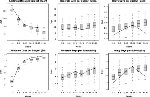
Figure 7: Posterior predictive checks of the mean and standard deviation of all three drinking outcomes in each of the six 4-week time periods during the trial. The gray shaded boxplots display the distributions of simulated values of each statistic, and the black lines display the observed values of these statistics. For example, for the first four weeks of the trial, the mean number of abstinent days across subjects was about 23 days, and in 1000 post-burn-in simulations, the value of this statistic ranged from approximately 21–24 days, indicating no major lack of fit with respect to this statistic.

7.4 Serial dependence comparison

To analyze the difference between the Markov model and the HMM(3), we look for patterns among the data in which one model fits better than the other. One striking such pattern is related to the way that the two models handle the serial dependence in the data. Their difference is apparent in the posterior distributions of the estimated probabilities (or, equivalently, the deviances) of certain data points. The HMM(3) fits better than the Markov model to the third data point in sequences of the form $(3,1,3)$, $(1,2,1)$, $(2,3,2)$, etc., where two days of equal consumption are interrupted by a single day of a different level of consumption. The Markov model, on the other hand, fits better than the HMM(3) to the third data point in sequences of the form $(3,1,1)$, $(1,2,2)$ and $(2,3,3)$, etc., where the second and third day’s consumption levels are equal to each other and different from the first day’s consumption.

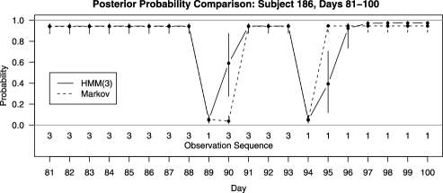
Figure 8: Point estimates and vertical 95% posterior intervals for the estimated probabilities of a sequence of data points for Subject 186 under both models, where the Markov model point estimates and intervals are drawn with dashed lines. Both models essentially fit equally well to the data in this sequence except for two points: the HMM(3) fits better to the heavy consumption on day 90, and the Markov model fits better to the abstinence on day 95.

Consider Figure 8, in which 95% intervals and point estimates of the posterior probabilities of a sequence of outcomes for Subject 186 are plotted for both the HMM(3) and the Markov model. On day 90, the third day of a $(3,1,3)$ sequence, the HMM(3) fits the data better, because the subject’s reported abstinence on day 89 did not necessarily represent a change in the hidden state during this sequence. On day 95, on the other hand, the Markov model fits the data better, because the reported abstinence that day was the first of many days in a prolonged sequence of abstinent behavior. In this case both models fit poorly to the unexpected day of abstinence on day 94, but the Markov model predicts the following day of abstinence with high probability, whereas the HMM(3) does more smoothing across time, and is therefore “slower” to predict the second abstinent day (on day 95). This pattern is generally true for all triplets of the form $(i,j,i)$ and $(i,j,j)$, where $i$ and $j$ represent observed consumption levels.

In the presence of measurement error—which is plausible given that the subjects self-report their alcohol consumption—and in light of the cognitive behavioral model of relapse, which suggests that a change in one’s alcohol consumption is not necessarily equivalent to a change in one’s underlying health state, the “smoother” fit of the HMM(3) is an advantage over the Markov model. The notion that the underlying behavior of individuals with an AUD is relatively steady, and that the observations are somewhat noisy, is consistent with the cognitive behavioral model of relapse.

7.5 Differences across subjects

To see the different drinking behaviors across subjects, we simulated sample paths from the fitted model for each subject using a procedure similar to the 4-step procedure outlined in Section 7.1. This time, however, instead of simulating new random effects, $\bolds{\alpha}^{\mathrm{rep}}$, from the posterior distributions of $\bolds{\mu}$ and $\bolds{\sigma}$ to represent a new sample of subjects from the population, we simply used the posterior samples of $\bolds{\alpha}$ directly to simulate new hidden states, $\mathbf{H}^{\mathrm{rep}}$, and observations, $\mathbf{Y}^{\mathrm{rep}}$ (steps 2 and 3 of the procedure). This way each set of simulated time series represents a new set of realizations for the exact same set of subjects whose data were observed, and we can make direct comparisons between the observed data and the simulations for each individual.

Figure 9 displays the observed drinking time series and one randomly drawn simulated time series for four subjects whose behaviors varied widely from each other. From the figure it is clear that the random effects in the HMM(3) allow it to capture a wide variety of drinking behaviors. Here is a summary of these four drinking behaviors:

1. Subject 89 is almost always abstinent, with occasional days of heavy drinking,

2. Subject 59 drinks heavily in very frequent short bursts (typically for just 1–2 days in a row),

3. Subject 79 drinks heavily on occasion for longer periods of time (10 days in a row appears typical),

4. Subject 5 drinks moderately for prolonged periods of time.

Each of these four unique drinking behaviors is captured by the HMM(3) through the random effects in the hidden state transition matrix.

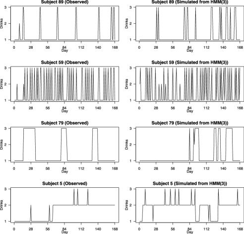
Figure 9: A visual comparison of observed (left column) and simulated (right column) time series for four subjects whose behavior varied widely. The HMM(3) is able to reproduce a wide variety of behaviors via its random effects in the hidden state transition matrix.

8 A new definition of relapse

The HMM offers a new definition of a relapse: any time point at which the probability is high that a subject is in hidden state 3, the Heavy Drinking state. There are a variety of ways to estimate the hidden states in an HMM, many of which are discussed in Scott (2002). Most methods can be categorized in one of two ways: They either maximize the marginal probability of each $H_{it}$ separately, or they attempt to find the set of sequences of hidden states $\mathbf{H}$ (which we think of as an $N\times T$ array, consisting of a set of $N$ sequences, each of length $T$) that is collectively the most likely (i.e., the mode of the joint posterior distribution of $\mathbf{H}$). The first method requires the calculation of the marginal probabilities of each hidden state at each time point, and then estimates the hidden state for each subject and time point as $\max_{s}\{\mathrm{P}(H_{it}=s|\mathbf{Y},\bolds{\theta})\}$. When the hidden state transition matrix contains zeroes, though, or has high probabilities on the diagonal (as it does in our case for many individuals), then using the marginal probabilities to estimate hidden states can result in a sequence that is very unlikely, or even impossible, because maximizing the marginal probabilities does not fully account for the dependence between consecutive hidden states [Rabiner and Juang (1986)]. Such a sequence is not appealing for characterizing relapse periods because our goal is to segment a subject’s drinking time series into plausible periods of in-control drinking behavior as opposed to out-of-control (relapse) drinking behavior.

We attempt the second type of hidden state estimation, in which we seek to find the set of sequences $\mathbf{H}$ that is the most likely, given the observed data. In the Bayesian framework, one way to do this would be to select the sequence $\mathbf{H}^{(g)}$ that occurs most often in our post-burn-in posterior samples $g=1,\ldots,G$. With such a large data set, though, it would require a huge number of MCMC iterations to ensure that a single realization of $\mathbf{H}$ was sampled twice or more. In our posterior sample, for example, the largest amount of overlap between any two samples of $\mathbf{H}$ was about 93% [that is, the pair of sets $(\mathbf{H}^{(i)},\mathbf{H}^{(j)})$ for $i,j\in(1,\ldots,G)$ that had the most elements in common shared about 93% of their elements]. Thus, to estimate $\mathbf{H}$, we used a different method: we computed the most likely set of sequences given the observed data and the posterior mean, $\bar{\bolds{\theta}}$, using the Viterbi algorithm [Rabiner and Juang (1986)]. This is similar to what is done is most frequentist analyses of HMMs, in which the Viterbi algorithm is run conditional on the MLEs of the model parameters to compute the most likely sequence(s) of hidden states.

Figure 10 shows the observed data and the most likely hidden states for two subjects. Subject 150 is estimated to be in the Heavy Drinking state from about Day 10 to about Day 140, despite not drinking on a number of days during that span. Likewise, Subject 186 is estimated to be in the Heavy Drinking state for a prolonged period of time despite a few days of abstinence during that time span. According to the definition of relapse that says any day spent in the Heavy Drinking hidden state is a relapse, these subjects were both in a state of relapse for a long, continuous period of time. This relapse definition is robust to outliers and measurement errors in the sense that a single day, or a brief “burst,” among the observations does not necessarily imply a transition in the most likely hidden state sequence. On many days, these two subjects reported a single day of abstinence, preceded and followed by many consecutive days of heavy drinking. Some definitions of relapse would be sensitive to these abstinence observations, and would suggest that the subject was no longer in a state of relapse, whereas the HMM-based definition of relapse includes these days as well, because the most likely hidden state sequence remains the same whether those observations were a 1, 2 or 3, because of the dependence structure across time that the HMM imposes.

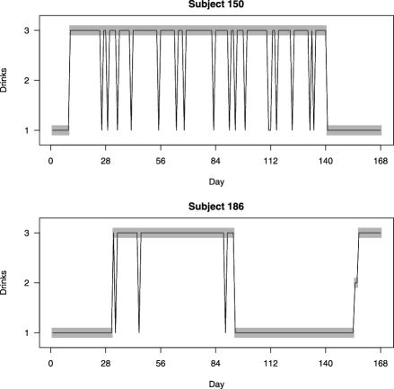
Figure 10: The most likely sequence of hidden states for Subjects 150 and 186. The dark lines represent the observed daily drink counts, and the shaded regions represent the estimated hidden state at each time point, where the hidden states are numbered 1 through 3 as they are in Table 2.

Using this definition of relapse, a relapse depends on one’s unobservable physical and mental state of health, rather than directly on one’s drinking behavior. Choosing which relapse definition is best for a given purpose requires clinical insight. Currently used definitions of relapse define what patterns of drinking constitute a relapse a priori before looking at the data. There is no consensus on what patterns constitute a relapse [Maisto et al. (2003)]. An advantage of the HMM approach is that it starts with a model of drinking behavior and a qualitative definition of relapse (e.g., a state in which a subject has a substantial probability of drinking heavily) and then lets the data decide what patterns of drinking constitute a relapse. This being said, we found evidence from earlier fits of HMMs to this data that the HMM-based definitions of relapse are sensitive to the number of hidden states in the model and the choice of which hidden states are categorized as relapse states. This choice becomes harder as the number of hidden states grows, because with more hidden states, the conditional distributions tend to correspond less clearly to easily identifiable drinking behaviors. Thus, using the HMM definition of relapse suggested in this section still requires careful thought on the part of the investigator with respect to (1), the choice of the number of hidden states, and, once that choice is made, to (2), the choice of which hidden states will be designated as relapse states.

9 Discussion and extensions

In this paper we develop a nonhomogenous, hierarchical Bayes HMM with random effects for data from a clinical trial of an alcoholism treatment. The model is motivated by data which exhibits flat stretches and bursts, as well as by the cognitive-behavioral model for relapse that coincides with the structure of the HMM, in which subjects make transitions through unobservable mental/physical states over time, and their daily alcohol consumption, which is observed, depends on their underlying state. A major strength of the HMM (and also of the Markov model we propose) is that it models the daily alcohol consumption of subjects. Such a model provides a rich description of subjects’ alcohol consumption behavior over time, as opposed to some lower-dimensional random variable such as the time until a subject’s first relapse, which provides a narrower view of a subject’s alcohol consumption.

The fit of the model to the data reveals a number of interesting things. The HMM with three hidden states fits well, and the hidden state transition matrix reveals that the most persistent state is abstinence, followed by heavy drinking, followed by moderate drinking. The transition matrices, however, vary widely among subjects, and the models, in general, are able to reproduce a wide variety of drinking behaviors (see Figure 9). The treatment in the clinical trial we analyzed, Naltrexone, appears to have a small, beneficial effect on certain transition probabilities, as well as on the overall percentage of time one would expect to spend in the heavy drinking state. Posterior predictive checks reveal that the heterogeneity among individuals is captured by the random effects in the hidden state transition matrices. Furthermore, the HMM(3) adequately models nonstationary, nonlinear and heteroscedastic drinking patterns across time.

Also, the HMM suggests a new definition of relapse, based on hidden states, which is conceptually supported by the cognitive-behavioral model of relapse, and can be compared to existing definitions of relapse to offer new insights into which patterns of drinking behavior are indicative of out-of-control behavior (i.e., a substantial probability of heavy drinking).

Appendix: MCMC algorithms to fit the models

Here we present some details of the MCMC algorithms used to fit the models.

.1 Fitting the Markov model

The Markov model, as was described in Section 3.2, is essentially composed of $M$ separate multinomial logit models, one for each row of the transition matrix. The Markov model, however, is substantially more difficult to fit, because the observations given the model parameters are not i.i.d.; each observation depends on the previous one. We incorporate a data augmentation step into the Metropolis-within-Gibbs algorithm to fit the Markov model. First, the priors:

$$\quad\beta_{mjk} \sim N(0,10^{2})\qquad\mbox{for }m=1,\ldots,M,j=2,\ldots,M,k=1,\ldots,p,$$ (7)

$$\quad\mu_{mj} \sim N(0,10^{2})\qquad\mbox{for }m=1,\ldots,M,j=2,\ldots,M,$$ (8)

$$\quad p(\sigma_{mj}) \sim 1\qquad\mbox{for }m=1,\ldots,M,j=2,\ldots,M,$$ (9)

$$\quad\bolds{\pi} \sim \operatorname{Dirichlet}(\mathbf{1}).$$ (10)

We fit the Markov model with the following steps:

1. Initialize the parameters, $\alpha_{ijm}^{(0)},\bolds{\beta}_{jm}^{(0)}$, for $i=1,\ldots,N$, $j=1,\ldots,M$, and $m=2,\ldots,M$, using overdispersed starting values, and initialize $\mu_{jm}^{(0)}=0$ and $\sigma_{jm}^{(0)}=1$ for $j=1,\ldots,M$, and $m=2,\ldots,M$.

2. For $g=1,\ldots,G$,

   1. [(c)]

   2. Sample $\mathbf{Y}_{i}^{\mathrm{mis},(g)}|\mathbf{Y}_{i}^{\mathrm{obs}},\bolds{\alpha}_{i}^{(g-1)},\bolds{\beta}^{(g-1)}$ from its full conditional distribution for $i=1,\ldots,N$.

   3. Sample $\alpha_{ijm}^{(g)}|\mathbf{Y}_{i}^{\mathrm{obs}},\mathbf{Y}_{i}^{\mathrm{mis},(g)},\bolds{\beta}_{j}^{(g-1)},\mu_{jm},\sigma_{jm}$ using a univariate random walk Metropolis sampler for $i=1,\ldots,N$, $j=1,\ldots,M$, and $m=2,\ldots,M$.

   4. Sample $\beta_{jmk}^{(g)}|\mathbf{Y}^{\mathrm{obs}},\mathbf{Y}^{\mathrm{mis},(g)},\bolds{\alpha}_{j}^{(g)}$ using a univariate random-walk Metropolis sampler, for $j=1,\ldots,M$, $m=2,\ldots,M$, and $k=1,\ldots,p$, where $\bolds{\alpha}_{j}^{(g)}$ denotes the $N\times(M-1)$ matrix of random intercepts sampled during iteration $g$.

   5. Sample $\mu_{jm}^{(g)}|\bolds{\alpha}_{jm}^{(g)},\sigma_{jm}^{(g-1)}$ from its full conditional normal distribution for $j=1,\ldots,M$ and $m=2,\ldots,M$, where $\bolds{\alpha}_{jm}^{(g)}$ is the length-$N$ vector of random intercepts sampled during iteration $g$.

   6. Sample $\sigma_{jm}^{(g)}|\bolds{\alpha}_{jm}^{(g)},\mu_{jm}^{(g)}$ from its full conditional inverse chi-squared distribution for $j=1,\ldots,M$ and $m=2,\ldots,M$.

   7. Sample $\bolds{\pi}|\mathbf{Y}^{\mathrm{obs}},\mathbf{Y}^{\mathrm{mis},(g)}$ from its full conditional Dirichlet distribution.

Given the full set of observations for each subject $(\mathbf{Y}_{i}^{\mathrm{obs}},\mathbf{Y}_{i}^{\mathrm{mis}})$, which we have after step (a) of each iteration, we easily sample the model parameters [steps (b)–(e) in the algorithm] associated with each row $j$ of the transition matrix by gathering all the observations $\{Y_{it}\in\mathbf{Y}_{(i,1:(T-1))}\dvtx Y_{it}=j\}$, and then treating the subsequent observations, $Y_{(i,t+1)}\in(1,2,\ldots,M),$ as draws from a multinomial distribution with probability distributions given in Equation (3), and we do this for rows $j=1,\ldots,M$.

.2 Fitting the HMM

The priors for the HMM are the same as they are for the Markov model, except we replace $M$ with $S$ in Equations (7)–(10), and we add the prior distributions for the parameters in the conditional distributions, $\mathbf{P}_{s}\sim\operatorname{Dirichlet}(\mathbf{1})$, for $s=1,\ldots,S$.

The HMM fit requires a similar, but slightly different Metropolis-within-Gibbs MCMC algorithm from that of the Markov model. We follow Scott (2002) and, in each iteration of the MCMC algorithm, use a forward-backward recursion to evaluate the likelihood, sample the hidden states given the parameters, and then sample the parameters given the hidden states. The details are as follows:

1. First, initialize all model parameters. For the HMM, we initialize the parameters in a specific way so as to avoid the label-switching problem that is common to fitting HMMs, and can be triggered by widely dispersed starting points. First, we fit the HMM with $S$ hidden states using the EM algorithm, without incorporating covariates and with complete pooling across subjects. We then set the values of $\bolds{\beta}_{rs}^{(0)}$ to zero, and set the values of $\mu_{rs}^{(0)}$ to the values such that, if all the $N$ random intercepts $\alpha_{irs}^{(0)}$, for $i=1,\ldots,N$, were set to equal $\mu_{rs}^{(0)}$, the model would have the same exact transition probabilities as MLE transition probabilities estimated from the EM algorithm. This usually ensures that each chain in a multichain MCMC algorithm converges to the same mode of the posterior distribution, which has $S!$ symmetric modes corresponding to the permutations of the state labels.

2. For $g=1,\ldots,G$,

   1. [(c)]

   2. Sample the vector $\mathbf{H}_{i}|\mathbf{Y}_{i}^{\mathrm{obs}},\bolds{\beta},\bolds{\alpha}_{i},\mathbf{P},\bolds{\pi}$ from it’s full conditional distribution using the forward-backward recursion as described in detail in Scott (2002), for $i=1,\ldots,N$.

   3. Sample $\bolds{\beta}$, $\bolds{\alpha}$, $\bolds{\mu}$ and $\bolds{\sigma}$ given $\mathbf{H}$ just as they are sampled in steps (b)–(e) in the Markov model, except replace the indices $j$ and $m$ with $r$ and $s$, respectively, for $r=1,\ldots,S$ and $s=2,\ldots,S$, and replace $(\mathbf{Y}^{\mathrm{obs}},\mathbf{Y}^{\mathrm{mis}})$ with $\mathbf{H}$.

   4. Sample $\mathbf{P}|\mathbf{H},\mathbf{Y}^{\mathrm{obs}}$ from its full conditional distribution.

   5. Sample $\bolds{\pi}|\mathbf{H}_{1}$ from its full conditional Dirichlet distribution, where $\mathbf{H}_{1}$ denotes the length-$N$ vector of hidden states at time $t=1$.

Data Files Included in the supplementary materials are two data files. The first file, “y.csv,” contains the ordinal drink counts for each subject on each day, and has $N=240$ rows and $T=168$ columns. The second file, “x.csv,” contains the covariates used to fit our models, and contains sex, treatment and prior drinking behavior for each subject.

Data Files [doi]10.1214/09-AOAS282SUPP [url]http://lib.stat.cmu.edu/aoas/282/supplement.zip .zip Included in the supplementary materials are two data files. The first file, “y.csv,” contains the ordinal drink counts for each subject on each day, and has $N=240$ rows and $T=168$ columns. The second file, “x.csv,” contains the covariates used to fit our models, and contains sex, treatment and prior drinking behavior for each subject.

References

- (1) Albert, P. (1999). A mover-stayer model for longitudinal marker data. Biometrics 55 1252–1257.
- (2) Albert, P. (2000). A transitional model for longitudinal binary data subject to nonignorable missing data. Biometrics 56 602–608.
- (3) Albert, P. (2002). A latent autoregressive model for longitudinal binary data subject to informative missingness. Biometrics 58 631–642. \MR1933536
- (4) Altman, R. J. (2007). Mixed hidden Markov models: An extension of the hidden Markov model to the longitudinal data setting. J. Amer. Statist. Assoc. 102 201–210. \MR2345538
- (5) Anton, R. F., et al. (2006). Combined pharmacotherapies and behavioral interventions for alcohol dependence. J. Amer. Medical Assoc. 295 2003–2017.
- (6) Cappe, O., Moulines, E. and Ryden, T. (2005). Inference in Hidden Markov Models. Springer, New York. \MR2159833
- (7) Cook, R. J., Kalbfleisch, J. D. and Yi, G. Y. (2002). A generalized mover-stayer model for panel data. Biostatistics 3 407–420.
- (8) Cox, D. R. (1981). Statistical analysis of time series: Some recent developments. Scand. J. Statist. 8 93–115. \MR0623586
- (9) Gelman, A. G., Carlin, J. B., Stern, H. S. and Rubin, D. B. (2004). Bayesian Data Analysis, 2nd ed. Chapman & Hall/CRC, New York. \MR2027492
- (10) Gelman, A. G. and Hill, J. (2007). Data Analysis Using Regression and Multilevel/Hierarchical Models. Cambridge Univ. Press, New York.
- (11) Humphreys, K. (1998). The latent Markov chain with multivariate random effects. Sociological Methods and Research 26 269–299.
- (12) Longford, N. T., Ely, M., Hardy, R. and Wadsworth, M. E. J. (2000). Handling missing data in diaries of alcohol consumption. J. Roy. Statist. Soc. Ser. A 163 381–402.
- (13) MacDonald, I. L. and Zucchini, W. (1997). Hidden Markov and Other Models for Discrete-Valued Time Series. Chapman & Hall, New York. \MR1692202
- (14) Maisto, S. A., Pollock, N. K., Cornelius, J. R., Lynch, K. G. and Martin, C. S. (2003). Alcohol relapse as a function of relapse definition in a clinical sample of adolescents. Addictive Behaviors 28 449–459.
- (15) Marlatt, G. A. and Gordon, J. R. (1985). Relapse Prevention: Maintenance Strategies in the Treatment of Addictive Behaviors. Guilford Press, New York.
- (16) McKay, J. R., Franklin, T. R., Patapis, N. and Lynch, K. G. (2006). Conceptual, methodological, and analytical issues in the study of relapse. Clinical Psychology Review 26 109–127.
- (17) Oslin, D. W., Lynch, K. G., Pettinati, H. M., Kampman, K. M., Gariti, P., Gelfand, L., Ten Have, T., Wortman, S., Dundon, W., Dackis, C., Volpicelli, J. R. and O’Brien, C. P. (2008). A placebo-controlled randomized clinical trials of naltrexone in the context of different levels of psychosocial intervention. Alcoholism: Clinical and Experimental Research 32 1299–1308.
- (18) Rabiner, L. R. and Juang, B. H. (1986). An introduction to hidden markov models. IEEE Acoustics, Speech, and Signal Processing 3 4–16.
- (19) Scott, S. (2002). Bayesian methods for hidden Markov models: Recursive computing in the 21st century. J. Amer. Statist. Assoc. 97 337–351. \MR1963393
- (20) Scott, S., James, G. M. and Sugar, C. A. (2005). Hidden Markov models for longitudinal comparisons. J. Amer. Statist. Assoc. 100 359–369. \MR2170459
- (21) Seltman, H. J. (2002). Hidden Markov models for analysis of biological rhythm data. In Case Studies in Bayesian Statistics 5 397–405. Springer, New York. \MR1931877
- (22) Shirley, K. E., Small, D. S., Lynch, K. G., Maisto, S. A. and Oslin, D. W. (2009). Supplement to “Hidden Markov models for alcoholism treatment trial data.” DOI: 10.1214/09-AOAS282SUPP.
- (23) Spiegelhalter, D. J., Best, N. G., Carlin, B. P. and van der Linde, A. (2002). Bayesian measures of model complexity and fit. J. Roy. Statist. Soc. Ser. B 64 583–639. \MR1979380
- (24) Velicer, W. F., Martin, R. A. and Collins, L. M. (1996). Latent transition analysis for longitudinal data. Addiction 91 (Supplement) S197–S209.
- (25) Wang, S. J., Winchell, C. J., McCormick, C. G., Nevius, S. E. and O’Neill, R. T. (2002). Short of complete abstinence: An analysis exploration of multiple drinking episodes in alcoholism treatment trials. Alcoholism: Clinical and Experimental Research 26 1803–1809.
- (26) Witkiewitz, K. and Marlatt, G. A. (2004). Relapse prevention for alcohol and drug problems. American Psychologist 59 224–235.