A multivariate adaptive stochastic search method for dimensionality reduction in classification

Abstract

High-dimensional classification has become an increasingly important problem. In this paper we propose a “Multivariate Adaptive Stochastic Search” (MASS) approach which first reduces the dimension of the data space and then applies a standard classification method to the reduced space. One key advantage of MASS is that it automatically adjusts to mimic variable selection type methods, such as the Lasso, variable combination methods, such as PCA, or methods that combine these two approaches. The adaptivity of MASS allows it to perform well in situations where pure variable selection or variable combination methods fail. Another major advantage of our approach is that MASS can accurately project the data into very low-dimensional non-linear, as well as linear, spaces. MASS uses a stochastic search algorithm to select a handful of optimal projection directions from a large number of random directions in each iteration. We provide some theoretical justification for MASS and demonstrate its strengths on an extensive range of simulation studies and real world data sets by comparing it to many classical and modern classification methods.

, and

1 Introduction

An increasingly important topic is the classification of observations into two or more predefined groups when the number of predictors, $d$, is larger than the number of observations, $n$. For example, one may need to identify at what time a subject is performing a specific task based on hundreds of thousands of brain voxel values in a functional Magnetic Resonance Imaging (fMRI) study, where changes in blood flow and blood oxygenation are measured when brain neurons are activated. In particular, the data set that motivated the development of the methodology in this paper was an fMRI study based on vision research. We wish to predict, at a given time, whether a subject is conducting a task or resting (baseline), based on the activity level of the observed voxels in the subject’s brain. This is a difficult task because the number of voxels, $d$, is much higher than the number of observations, $n$. In this case, many conventional classification methods, such as Fisher’s discriminant rule, are not applicable since $n<d$. Other methods, such as classification trees, $k$-nearest neighbors and logistic discriminant analysis, do not explicitly require $n>d,$ but in practice provide poor classification accuracy in this situation.

A common solution is to first reduce the data into a lower, $p\ll d$ dimensional space and then perform classification on the transformed data. For example, Fan and Lv (2008) provide significant theoretical and empirical evidence for the power of such an approach. Generally, the dimension reduction is performed using a linear transformation of the form

$$\mathbf{Z}=\mathbf{X}\mathbf{A},$$ (1)

where $\mathbf{X}$ is an $n$-by-$d$ data matrix and $\mathbf{A}$ is a $d$-by-$p$ transformation matrix which projects $\mathbf{X}$ onto a $p$-dimensional subspace $\mathbf{Z}~{}(p<d)$. However, there are many possible approaches to choosing $\mathbf{A}$. We divide the methods into supervised versus unsupervised and variable selection versus variable combination.

Variable selection techniques select a subset of relevant variables that have good predictive power, thus obtaining a subset of informative variables from a set of more complex variables. In this setting, $\mathbf{A}$ is some row permutation of the identity matrix and the zero matrix, that is, $\mathbf{A}=\operatorname{perm}([\mathbf{I}_{p},\mathbf{0}_{(d-p)\times p}]^{T})$. If we define sparsity as the fraction of zero elements in a given matrix, then $\mathbf{A}$ would be considered sparse because most of its components are zeros. Many variable selection methods have been proposed and widely used in numerous areas. A great deal of attention is paid to the $L_{1}$ penalized least squares estimator [i.e., the Lasso Tibshirani (1996), Efron et al. (2004)]. Other methods include SCAD Fan and Li (2001), nearest shrunken centroids Tibshirani et at. (2002), the Elastic Net Zou and Hastie (2005), Dantzig selector Candes and Tao (2007), VISA Radchenko and James (2008), FLASH Radchenko and James (2009) and Bayesian methods of variable selection Mitchell and Beauchamp (1988), George and McCulloch (1993, 1997). These methods all use supervised learning, where the response and predictors are both utilized to obtain the subset of variables. In addition, because these methods always select a subset of the original variables, they provide highly interpretable results. However, because of the sparsity of $\mathbf{A}$, for a given $p$, variable selection methods are less efficient at compressing the observed data, $\mathbf{X}$. For example, they may discard potentially valuable variables which are not predictive individually but provide significant improvement in conjunction with others.

In comparison, variable combination methods utilize a dense $\mathbf{A}$ which combines correlated variables and hence does well on multicollinearities which often occur in high-dimensional data. Probably the most commonly applied method in this category is principal component analysis (PCA). Using this approach, $\mathbf{A}$ becomes the first $p$ eigenvectors of $\mathbf{X}$, and $\mathbf{Z}$ is the associated PCA scores. PCA can deal with an ultra large data scale and produces the most efficient representation of $\mathbf{X}$ using $p$ dimensions. However, PCA is an unsupervised learning technique which does not make use of the response variable to construct $\mathbf{A}$. It is well known that the dimensions that best explain $\mathbf{X}$ will not necessarily be the best dimensions for predicting the response $Y$. Other variable combination methods include partial least squares regression and multidimensional scaling. All these approaches yield linear combinations of variables which makes interpretation more difficult.

In this paper we propose a new supervised learning method which we call “Multivariate Adaptive Stochastic Search” (MASS). Our approach works by projecting a high dimensional data set into a lower dimensional space and then applying a classifier to the projected data. However, MASS has two key advantages over these other methods. First, when using a linear projection, such as given by (1), MASS uses a stochastic search process that is capable of automatically adapting the sparsity of $\mathbf{A}$ to generate optimal prediction accuracy. Hence, in situations where a subset of the original variables provides a good fit, MASS will utilize a sparse model, while in situations where linear combinations of the variables work better, MASS will produce a denser model. MASS has the same advantage as other supervised methods in which $\mathbf{A}$ can be designed specifically to provide the best level of prediction accuracy. However, it has the flexibility to adapt the sparsity of $\mathbf{A}$ so as to gain the benefits of both the variable selection and variable combination methods. The second major advantage of MASS is that, with only a small adaption to the standard fitting procedure, it can project the original data into a nonlinear space. This generalization of (1) potentially allows for a very accurate projection into a low-dimensional space with little additional effort.

MASS starts by generating a large set of prospective columns for $\mathbf{A}$ with a given sparsity level. A variable selection technique such as the Lasso is then applied to select a candidate subset of “good” columns or directions. Then, a new set of columns with a new sparsity level are produced as candidates. The variable selection method must choose among the current set of good columns and the new candidates. Over time the same best columns are picked at each iteration and the process converges. At each step in the algorithm, the sparsity level of the new prospective columns is adjusted according to the sparsity level of the previously chosen columns. We show through extensive simulations and real world examples that MASS is highly robust in that it generally provides comparable performance to variable selection and variable combination approaches in situations that favor each of these methods. However, MASS can still perform well in situations where one or another of these approaches fails.

This paper is organized as follows. In Section 2 we present the basic MASS methodology. After outlining the linear fitting algorithm, we show how this can easily be extended to the nonlinear generalization. Furthermore, we provide some theoretical motivation for MASS and discuss a preliminary data reduction which can be implemented before applying MASS. In Section 3 we demonstrate the performance of MASS on an fMRI study and a gene microarray study. In Section 4 we further study the performance of MASS on different scenarios by comparing MASS with several other modern potential classification techniques, such as $k$-nearest neighbors, support vector machines, random forests and neural networks, in extensive simulation studies. We briefly investigate some issues in implementing MASS, such as solution variability, computational cost and the problem of overfitting, in Section 5. A brief discussion summarizes the paper in Section 6.

2 Projection selection with MASS

2.1 General ideas and motivations

Given predictors, $\mathbf{x}_{i}\in\mathbb{R}^{d}$, and corresponding categorical responses, $y_{i}$, we model the relationship between $y_{i}$ and $\mathbf{x}_{i}$ as

$$y_{i}|\mathbf{x}_{i} \sim g(y_{i}|\mathbf{z}_{i}),\qquad i=1,\dots,n,$$ (2)

$$z_{i,j} = f_{j}(\mathbf{x}_{i}),\qquad j=1,\dots,p,$$ (3)

where $\mathbf{z}_{i}=(z_{i,1},\dots,z_{i,p})$ for some $p\ll d$. Our general approach is to estimate the $f_{j}$’s, project the data into a lower $p$-dimensional sub-space, $\mathbf{z}_{i}$, and then apply a standard classification method to fit (2).

To make this problem tractable, we further assume that $f_{j}$ has an additive structure, $f_{j}(\mathbf{x}_{i})=\sum^{d}_{k=1}f_{j,k}(x_{i,k})$, and, hence, (3) becomes

$$z_{i,j}=\sum^{d}_{k=1}f_{j,k}(x_{i,k}).$$ (4)

For any given $z_{i,j}$ and $x_{i,k}$’s, there are many functions, $f_{j,k}$, that satisfy (4). However, to solve Equation (4), we constrain the flexibility of these functions by imposing the constraints, $f_{j,k}(0)=0$, and

$$\int f_{j,k}^{\prime\prime}(x)^{2}\,dx\leq\lambda,\qquad j=1,\ldots,p,k=1,\ldots,d,\lambda\leq 0.$$ (5)

It should be noted that Equation (5) can trivially be made to hold by rescaling $f_{j,k}$. To prevent this occurring, we impose a further constraint on the first derivative of the $f_{j,k}$’s, when $f_{j,k}$’s are nonlinear; details are proved in Appendix B. Using equation (5), small values of $\lambda$ constrain $f_{j,k}$ to be close to a linear function. In particular, setting $\lambda=0$ implies $f_{j,k}(x)=a_{j,k}x$, in which case (3) reduces to the linear projection given by (1). We first describe the linear MASS approach for fitting (2) and (4) subject to $\lambda=0$ and then in Section 2.4 show how the procedure can easily be extended to the more general nonlinear case when $\lambda>0$.

In the linear situation fitting our model given by (2) through (4) requires choosing the $f_{j,k}$’s, or equivalently estimating $\mathbf{A}$ in (1), and also selecting a classifier to apply to the lower dimensional data. We place most attention on the former problem because there are many classification techniques that have been demonstrated to perform well on low-to-medium dimensional data. A more difficult question involves the best way to produce the lower dimensional data. Hence, we assume that one of these classification methods has been chosen and concentrate our attention on the choice of $\mathbf{A}$. This choice can be formulated as the following optimization problem:

$$\mathbf{A}=\arg\min_{\mathbf{A}}E_{\mathbf{X},Y}[e(\mathcal{M}_{\mathbf{A}}(\mathbf{X}),Y)]$$ (6)

$$\mbox{subject to }\quad\|\mathbf{a}_{j}\|=1,$$

where $\mathcal{M}_{\mathbf{A}}$ is the classification method applied to the lower dimensional data, ${\mathbf{X}}$ and $Y$ are the predictors and response variables, and $e$ is a loss function resulting from using $\mathcal{M}_{\mathbf{A}}$ to predict $Y$. The constraint is that each column of $\mathbf{A}$ should be norm 1. A common choice for $e$ is the $0$–$1$ loss function which results in minimizing the misclassification rate (MCR). Since $\mathbf{A}$ is high dimensional, solving (6) is in general a difficult problem.

There are several possible approaches to optimize (6). One option is to assume that $\mathbf{A}$ is a sparse $0,1$ matrix and only attempt to estimate the locations of its non-zero elements. This is the approach taken by variable selection methods. Another option is to assume $\mathbf{A}$ is dense but, instead of choosing $\mathbf{A}$ to optimize (6), select a matrix which provides a good representation for $\mathbf{X}$. This is the approach taken by PCA. One then hopes that the PCA solution will be close to that of (6).

Instead of making restrictive assumptions about $\mathbf{A}$, as with the variable selection approach, or failing to directly optimize (6), as with the PCA approach, we attempt to directly fit (6) without placing restrictions on the form of $\mathbf{A}$. In this type of high dimensional nonlinear optimization problem, stochastic search methods, such as genetic algorithms and simulated annealing, have been shown to provide superior results over more traditional deterministic procedures because they are often able to more effectively search large parameter spaces, can be used for any class of objective functions and yield an asymptotic guarantee of convergence Gosavi (2003), Liberti and Kucherenko (2005). We explore a stochastic search process and demonstrate that it is highly effective at searching the parameter space and generally requires significantly fewer iterations than other possible stochastic approaches Tian, Wilcox and James (2009).

2.2 The MASS method

The linear MASS procedure works by successively generating a large number, $L$, of potential random directions, that is, $\mathbf{a}_{j}$’s. We then use Equation (1) to compute the corresponding $L$ dimensional data space, $\mathbf{z}_{1},\mathbf{z}_{2},\ldots,\mathbf{z}_{L}$, and use a variable selection method to select a “good” subset of these directions to form an initial estimate, $\mathbf{A}^{*}$. The sparsity level of this $\mathbf{A}^{*}$ is examined and a new random set of potential columns is generated with the same average sparsity as the current $\mathbf{A}^{*}$. The procedure iterates in this fashion for a fixed number of steps. Formally, the MASS procedure consists of the following steps:

1. [Step 5.]

2. Randomly generate the initial $d$-by-$L$ transformation matrix $\mathbf{A}^{*(0)}$ $(p<L<d)$ with an expected sparsity of $\bar{\xi}^{(0)}$.

3. At the $l$th iteration, use Equation (1) and $\mathbf{A}^{*(l)}$ to obtain a preliminary reduced data space $\mathbf{Z}^{*(l)}$. Evaluate each variable of $\mathbf{Z}^{*(l)}$ by fitting a model $Y\sim\mathbf{Z}$, and select the $p$ most “important” variables in terms of the model.

4. Keep the corresponding $p$ columns of $\mathbf{A}^{*(l)}$ and calculate the average sparsity, $\bar{\xi}^{(l)}$, for these columns.

5. Generate $L-p$ new columns with an average sparsity of $\bar{\xi}^{(l)}$. Join these columns with the $p$ columns selected in Step 3 to form a new transformation matrix $\mathbf{A}^{*(l+1)}$.

6. Return to Step 2 for a fixed number of iterations.

Implementing this approach requires the choice of a variable selection procedure for Step 2. Potentially any of a large range of standard methods can be chosen. We discuss various options in Section 2.6.

A more crucial part of implementing MASS is the mechanism for generating the potential columns for $\mathbf{A}^{*}$. We define the current level of sparsity, $\bar{\xi}^{(l)}$, as the fraction of zero elements in $\mathbf{A}^{(l)}$. Then at each iteration of MASS we generate new potential columns with the same average sparsity level as the columns selected in the previous step. This allows $\bar{\xi}^{(l)}$ to automatically adjust to the data set. The idea is that a data set requiring high $\bar{\xi}^{(l)}$ will tend to result in sparser columns being selected and the current $\mathbf{A}$ will become sparser at each iteration. Alternatively, a data set that requires a denser $\mathbf{A}$ will select dense columns at each iteration. While at each step of the stochastic search the overall average sparsity is restricted to equal $\bar{\xi}^{(l)}$, we desire some variability in the sparsity levels so that MASS is able to select out columns with higher or lower sparsity and hence adjust $\bar{\xi}^{(l)}$ for the next iteration. To achieve this goal, we allow for different average sparsity levels between columns.

In particular, we generate the $(k,j)$th element of $\mathbf{A}^{*}$ using

$$a_{k,j} = u_{k,j}v_{k,j},\qquad k=1,\dots,d,j=p+1,\dots,L,$$ (7)

$$u_{k,j} \sim \mathcal{N}(0,1),\qquad v_{k,j}\sim\mathcal{B}(1-\xi_{j}),$$ (8)

where $\mathcal{B}(\pi)$ is the Bernoulli distribution with probability of $1$ equal to $\pi$. In the $(l+1)$th iteration, we let

$$\xi^{(l+1)}_{j}\sim\operatorname{Beta}\biggl{(}\alpha,\frac{\alpha(1-\bar{\xi}^{(l)})}{\bar{\xi}^{(l)}}\biggr{)},\qquad j=p+1,\ldots,L,$$ (9)

where $\xi^{(l+1)}_{j}$ is the sparsity of the $j$th column of $\mathbf{A}^{*(l+1)}$. Note that $E(\xi^{(l+1)}_{j})=\bar{\xi}^{(l)}$ for all values of $\alpha$. We found $\alpha=5$ produced a reasonable amount of variance in sparsity levels.

We then combine these $L-p$ columns with the selected $p$ columns from iteration $l$ to form the new intermediate transformation matrix $\mathbf{A}^{*(l+1)}$. We select $\bar{\xi}^{(0)}=0.5$ for the initial sparsity level, which seems to provide a reasonable compromise between the variable selection and variable combination paradigms.

The full MASS algorithm is explicitly described as follows:

1. Set $\bar{\xi}^{(0)}=0.5$ and generate an initial $\mathbf{A}^{*(0)}$ using (7) through (9). Calculate $\mathbf{Z}^{*(0)}$ by Equation (1).

2. Select $p$ variables from $\mathbf{Z}^{*(0)}$ and keep the corresponding $p$ columns from $\mathbf{A}^{*(0)}$ to obtain $\mathbf{A}^{(0)}$.

3. Iterate until $l=I$.

   1. [(c)]

   2. Generate $L-p$ new directions $\mathbf{A}^{*}_{\mathrm{new}}$ by using (7) through (9).

   3. Let $\mathbf{A}^{*(l)}=(\mathbf{A}^{(l-1)},\mathbf{A}^{*}_{\mathrm{new}})$ and use Equation (1) to obtain $\mathbf{Z}^{*(l)}$.

   4. Select $p$ variables from $\mathbf{Z}^{*(l)}$.

   5. Keep the corresponding $p$ columns from $\mathbf{A}^{*(l)}$ to obtain $\mathbf{A}^{(l)}$.

   6. Calculate $\bar{\xi}^{(l)}$ for $\mathbf{A}^{(l)}$.

   7. Go to (a).

4. Apply the selected classification technique to the final $\mathbf{Z}^{(I)}$.

2.3 Theoretical justification

Here we show that MASS will asymptotically select the correct sub-space, provided a “reasonable” variable selection method is utilized in Step 3(c). Assumption 1 below formally defines reasonable. Suppose our variable selection method must choose among $\mathbf{z}_{1},\ldots,\mathbf{z}_{L}$ potential variables. Let $\mathbf{Z}_{0}\in\mathbb{R}^{n\times p}$ represent the $p$-dimensional set of true variables. Note $\mathbf{Z}_{0}$ is not necessarily a subset of $\mathbf{z}_{1},\ldots,\mathbf{z}_{L}$. Define $\tilde{\mathbf{Z}}_{n}\in\mathbb{R}^{n\times p}$ as the $p$ variables among $\mathbf{z}_{1},\mathbf{z}_{2},\ldots,\mathbf{z}_{L}$ that minimize $\|\tilde{\mathbf{Z}}_{n}-\mathbf{Z}_{0}\|^{2}$ for a sample of size $n$. Then we assume that the variable selection method chosen for MASS satisfies the following property:

Assumption 1

There exists some $\varepsilon>0$ such that, provided

$$\frac{1}{n}\|\tilde{\mathbf{Z}}_{n}-\mathbf{Z}_{0}\|^{2}\leq\varepsilon,$$ (10)

then $\tilde{\mathbf{Z}}_{n}$ is chosen by the variable selection method almost surely as $n\rightarrow\infty$.

Assumption 1 is a natural extension of the definition of consistency of a variable selection method, namely, that it asymptotically selects the correct model. Here we extend this idea slightly by assuming that, provided a set of candidate predictors that is arbitrarily close to the true predictors is presented, the variable selection method will asymptotically choose these variables. Theorem 1 provides some theoretical justification for the MASS methodology.

Theorem 1

Let $\tilde{\mathbf{Z}}_{n}^{(I)}$ represent the $p$ variables selected by MASS after performing $I$ iterations on a sample of size $n$. Then, under the linear subspace model given by (1) and (2), provided a variable selection method is chosen such that Assumption 1 holds, as $n$ and $I$ approach infinity,

$$\frac{1}{n}\big{\|}\tilde{\mathbf{Z}}_{n}^{(I)}-\mathbf{Z}_{0}\big{\|}^{2}\rightarrow 0\qquad a.s.$$

The proof of Theorem 1 is given in Appendix A. Theorem 1 guarantees that, provided a reasonable variable selection method is chosen, then the sub-space chosen by MASS will converge to the “true” sub-space, in terms of mean squared error, as $n$ and $I$ converge to infinity. Note, Theorem 1 does not assume that (10) holds; Only that, if it does hold, then asymptotically $\tilde{\mathbf{Z}}_{n}$ will be selected.

2.4 The nonlinear generalization

Recently, nonlinear reduction work has mostly concentrated on local neighborhood methods such as Isomap Tenenbaum, de Silva and Langford (2000) and LLE Roweis and Saul (2000). One limitation of these approaches is that they are clustering based and hence are unsupervised methods. Another limitation is that these approaches only consider local feature spaces. They perform well when the data belong to a single well sampled cluster, but fail when the points are spread among multiple clusters. MASS can also produce a nonlinear reduction without the aforementioned problems.

Recall that MASS attempts to compute the $f_{j,k}$’s subject to (5) holding for some $\lambda\geq 0$. It is not hard to show that, among all functions that interpolate a given set of points, the one that minimizes the integrated squared second derivative will always be a natural cubic spline Reinsch (1967). Hence, since we wish to choose a set of functions that reproduce the $z_{i,j}$’s subject to (5), it seems sensible to model each $f_{j,k}$ using a $q$-dimensional natural cubic spline (NCS) basis, $\mathbf{b}(t)$.

Using this formulation, (4) becomes $z_{i,j}=\sum_{k=1}^{d}f_{j,k}(x_{i,k})=\sum^{d}_{k=1}\mathbf{b}(x_{i,k})^{T}\times\break\bolds{\theta}_{j,k}$, where $\bolds{\theta}_{j,k}$ represents the basis coefficients for $f_{j,k}$. Since the $z_{i,j}$’s are just linear functions of the $\bolds{\theta}$’s, we can rewrite (4) in the simpler linear form, (1),

$$\mathbf{Z}=\mathbf{X}^{*}\Theta,$$ (11)

where $\mathbf{X}^{*}=(B(\mathbf{x}_{1})|B(\mathbf{x}_{2})|\cdots|B(\mathbf{x}_{d}))\in\mathbb{R}^{n\times(q\times d)}$, $\Theta=(\bolds{\theta}_{1},\dots,\bolds{\theta}_{p})\in\mathbb{R}^{(q\times d)\times p}$, $\bolds{\theta}_{j}=(\theta^{T}_{j,1},\dots,\theta^{T}_{j,d})^{T}$, and $B(\mathbf{x}_{k})=(\mathbf{b}(x_{1,k}),\dots,\mathbf{b}(x_{n,k}))^{T}$.

The only complication in using the standard linear MASS methodology to fit (11) is ensuring that (5) holds. However, in Appendix B we show that some minor adaptations to (8) ensure that (5) holds for all candidate $\theta$’s that we generate. This is one of the advantages of the stochastic search process—it is easy to search only the feasible values of the $\Theta$ space. In all other respects, the MASS methodology as outlined in Section 2.2 can be applied without any alterations to estimate a non-linear sub-space of the data. It should also be noted that Theorem 1 can be extended to the nonlinear setting, provided we assume that the true nonlinear sub-space satisfies (5).

2.5 Preliminary reduction

MASS can, in general, be applied to any data. However, Fan and Lv (2008) argue that a successful strategy to deal with ultra-high dimensional data is to apply a series of dimension reductions. In our setting this strategy would involve an initial reduction of the dimension to a “moderate” level followed by applying MASS to the new lower dimensional data. This two stage approach potentially has two major advantages. First, Fan and Lv (2008) show that prediction accuracy can be considerably improved by removing dimensions that clearly appear to have no relationship to the response. Our own simulations reinforce this notion. Second, stochastic search algorithms such as MASS can require significant computational expense. Reducing the data dimension before applying MASS provides a large increase in efficiency.

In this paper we consider three methods for reducing the data into $m$ $(m>p)$ dimensions. The first approach is conventional PCA, which has the effect of selecting the best $m$ dimensional space in terms of minimizing the mean squared deviation with the original $d$ dimensional space. The second approach is the sure independence screening (SIS) method based on correlation learning Fan and Lv (2008). It computes the componentwise marginal correlations between each predictor and the response vector. One then selects the variables corresponding to the $m$ largest correlations. PCA is an unsupervised variable combination approach, while SIS is a supervised variable selection method. PCA may exclude important information among variables with less variability, while SIS may tend to select a redundant subset of predictors that have high correlations with the response individually but are also highly correlated among themselves. Our third dimension reduction approach, which we call PCA-SIS, attempts to leverage the best of both PCA and SIS by first using PCA to obtain $n$ orthogonal components and then treating these components as the predictors and using SIS to select the best $m$ in terms of correlation with the response. PCA-SIS can be thought of as a supervised version of PCA. We compare these three types of preliminary reduction methods, along with the effect of performing no initial dimension reduction, in our simulation studies.

Fan and Lv (2008) argue that the dimension of the intermediate space $m$ should be chosen as

$$m=\frac{2n}{\log(n)}.$$ (12)

As we have found that this approach generally works well, we have adopted Equation (12) for selecting $m$ in this paper.

2.6 Implementation issues

MASS requires the choice of a variable selection technique. In principle, any variable selection technique can be applied here. We considered several possible methods. In the context of classification, a natural approach is to use a GLM version of the Lasso using a logistic regression framework. We examined this approach using the GLMpath methodology of Park and Hastie (2007). Interestingly, we found that simply using the standard Lasso procedure to select the variables gave similar levels of accuracy to GLMpath and required considerably less computational effort. Therefore, in our implementation of MASS we use the first $p$ variables selected by the Lars algorithm Efron et al. (2004). However, in practice, one could implement our methodology with any standard variable selection method such as SCAD, Dantzig selector, etc. There is an extensive literature examining the circumstances under which the Lasso will asymptotically select the correct model [see, e.g., Knight and Fu (2000), Tsybakov and van de Geer (2005)]. Hence, it seems reasonable to suppose that Assumption 1 in Section 2.3 will hold.

To implement MASS, one must choose values for the number of iterations, $I$, the number of random columns to generate, $L$, and the final number of columns chosen, $p$. In our experiments we used $I=500$ iterations. We found this value guaranteed a good result and often fewer iterations were required. In general, tracking the deviance of the Lasso at each iteration provided a reliable measure of convergence. The value of $L$ influences the convergence speed of the algorithm as well as the execution time. We found that the best results were obtained by choosing $L$ to be a relatively large value for the early iterations but to have it decline over iterations. In particular, we set $L=n/2$ for the first iteration and had it decline to $2p$ by the final iteration. This approach is similar in spirit to simulated annealing where the temperature is lowered over time. It guarantees that the Lasso has more variables to choose from at the early stages, but then as the search moves toward the optimum, decreasing $L$ will improve the reliability of the selected $p$ variables in addition to speeding up the algorithm.

The choice of $p$ can obviously have an important impact on the results. In general, $p$ should be chosen as some balance of the classification accuracy and the computational expense. One reasonable approach is to use an objective criterion to choose $p$, such as cross-validation (CV). In other situations, some prior knowledge can be applied to select $p$. For example, in the fMRI study that we examine in Section 3, prior knowledge and assumptions on the regions of interest can be used to decide on a reasonable value for $p$.

3 Applications

In this section we apply linear MASS to two data sets from real studies: an fMRI data set and a gene microarray data set. As a comparison to MASS, we also apply classic logistic regression (LR) or support vector machine (SVM) to the lower dimensional data produced using a straight Lasso method (Lars), a generalized Lasso method (GLMpath), SIS and PCA. They all utilize equation (1) but compute ${\bf A}$ directly using their own methodologies. In both studies, we use 500 iterations for MASS.

3.1 fMRI brain imaging data

The fMRI data was obtained from the imaging center at the University of Southern California. The raw data consisted of 200 3-D brain images recording the blood oxygen level dependent (BOLD) response for a subject who was conducting a visual task. After preprocessing, each image contained 11,838 voxels. One research question was to divide the 200 images into task (96) and baseline (104) images based on the 11,838 voxels. To answer this question, we randomly divided the data to training (150) and test (50) samples. Since $d\gg n$, a preliminary reduction was needed. The intermediate scale was $m=60$ by Equation (12). We tested $p=10,20,30,40,50,60$, which were considered to be good balances of the execution time and the classification accuracy. SVM was used as the base classifier.

Table 1: Test MCR^∗ and $p^{*}$ on fMRI data using SVM

Methods	Test MCR$\bolds{{}^{*}}$	Optimal $\bolds{p^{*}}$
Lars	0.20	50
GLMpath	0.22	50
SIS	0.40	30
PCA	0.26	40
SIS-Lars	0.36	30
PCA-Lars	0.22	40
PCA-SIS-Lars	0.12	50
SIS-GlMpath	0.38	30
PCA-GLMpath	0.22	40
PCA-SIS-GLMpath	0.10	50
SIS-MASS	0.373 (0.008)	50
PCA-MASS	0.155 (0.005)	40
PCA-SIS-MASS	0.042 (0.005)	50

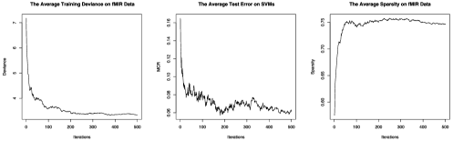
Figure 1: Preliminary reduction by PCA-SIS-MASS on fMRI data $(p=30)$.

Table 1 reports the minimum test MCR, MCR^∗, and its corresponding $p$, $p^{*}$, for each method. For each $p$, we applied MASS twenty times on the training data and obtained the average MCR on the test data. We then reported the minimum average test MCR, and its corresponding $p$. In this table as well as in the rest of the paper, SIS-MASS means that we first used SIS to reduce the data and then applied MASS. Similarly, PCA-SIS-Lars means that PCA-SIS was the first reduction method and then Lars was applied, etc.

Obviously, PCA-SIS-MASS dominates other methods. We show the training deviance, the average test MCR and the average sparsity as some function of the number of iterations in Figure 1. As we can see, the training deviance and the average test MCR decline rapidly and then level off, indicating the model improves quickly. The average $\bar{\xi}$ path for PCA-SIS-MASS indicates MASS chose a relatively sparse matrix as the optimal transformation matrix. We also examined the relative performance of MASS in comparison to a representative sampling of some modern classification methods [Support Vector Machines (SVM), $k$-Nearest Neighbors (kNN), Neural Networks (NN) and Random Forests (RF)] on the $m$-dimensional preliminary reduced data. As shown in Table 2, all four methods were inferior to MASS.

3.2 Leukemia cancer gene microarray data

The second real-world data set was the leukemia cancer data from a gene microarray study by Golub et al. (1999). This data set contained $72$ tissue samples, each with 7129 gene expression measurements and a cancer type label. Among the $72$ tissues, $25$ were samples of acute myeloid leukemia (AML) and $47$ were samples of acute lymphoblast leukemia (ALL). Within the $38$ training samples, $27$ were ALL and $11$ AML. Within the $34$ test samples, $20$ were ALL and $14$ AML. In some previous studies Fan and Fan (2008), Fan and Lv (2008), $16$ genes were ultimately chosen. In this study, we also picked $p=16$ genes for MASS. However, for the other counterpart methods, we examined all possible $p$’s, that is, $p=1,2,\ldots,21$, to obtain MCR^∗ and their corresponding $p^{*}$’s. This is considered to be an advantage for the counterpart methods and a disadvantage for MASS. The intermediate dimension was chosen to be $m=21$ by Equation (12). A LR model was applied for classification. Similar to the fMRI study, PCA-SIS-MASS provided the lowest MCR (see Table 3), and it was better than the nearest shrunken centroids method mentioned in Tibshirani et at. (2002), which obtained a MCR of $2/34=0.059$ based on $21$ selected genes Fan and Lv (2008). Figure 2 shows the resulting graphs. The sparsity of the transformation matrix leveled off at about $0.41$.

Table 2: Test MCR on the preliminary reduced data by different classifiers

	SVM	kNN	NN	RF
SIS-	0.36	0.40	0.44	0.34
PCA-	0.26	0.26	0.38	0.22
PCA-SIS-	0.24	0.20	0.36	0.20

Table 3: Test MCR^∗ and corresponding $p^{*}$ or standard errors (in the parentheses) on leukemia cancer data using LR

	Lars	GLMpath	MASS ($\bolds{p=16}$)
$m=21$
SIS-	$0.147\ (p^{*}=12,14\mbox{--}17,19,20)$	$0.088\ (p^{*}=16,17,20,22\mbox{--}24)$	0.176 (0.010)
PCA-	$0.029\ (p^{*}=13,15\mbox{--}17)$	$0.029\ (p^{*}=9)$	0.056 (0.008)
PCA-SIS-	$0.029\ (p^{*}=16)$	$0.029\ (p^{*}=15)$	0.004 (0.002)

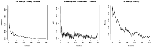
Figure 2: PCA-SIS-MASS on leukemia cancer data.

4 Simulation studies

In this section we further investigate the performance of MASS under different conditions. We give five simulation examples. The first simulation investigates the nonlinear setting, while the remaining simulations concentrate on the linear case. In all simulations we show results with MASS applied using the LR classifier and the SVM classifier. In addition, we also apply LR and SVM to the original full dimensional data (FD) and to lower dimensional data produced using Lars, GLMpath, SIS and PCA.

4.1 Simulation study I: Nonlinear data

In this setting we simulated data using the nonlinear additive model assumed by MASS. We first selected an NCS basis and then generated $\theta_{j,k}$’s such that (5) holds for a given $\lambda$. We used the same generation scheme as that used by the MASS algorithm. Details of the generation process are provided in Appendix B.

We simulated 20 training samples, each containing $100$ observations and $50$ predictor variables generated from $\mathcal{N}(0,\mathbf{I})$. The binary response variable was associated with the true $\mathbf{Z}_{0}\in\mathbb{R}^{n\times p_{0}}$ using a standard logistic regression model. Here we let $p_{0}=2$. For each training data set a corresponding set of $1000$ observations was generated as a test sample. In order to demonstrate the importance of the sparsity of the transformation matrix to the classification performance, we also implemented a modified version of MASS where we fixed the sparsity of the transformation matrix, $\bar{\xi}$, so that it did not change over iterations. We call this method the multivariate fixed stochastic search (MFSS) method. Presumably, MFSS with a good value of sparsity will perform better than MASS, because MASS has to adaptively search for $\bar{\xi}$. For MASS and MFSS, we let $p=p_{0}=2$ dimensions.

We considered two scenarios, where the true curvatures were $\lambda_{0}=5$ and $\lambda_{0}=10$. According to Equation (5), $\lambda$ is one of the indicators of the model complexity. With a larger $\lambda$, the model is more complex. The true sparsity for both scenarios were $\bar{\xi}_{0}=0.3$. The counterpart methods are Lars and PCA with their optimal $p^{*}$’s. We examined all possible values for $p$, that is, $p=1,2,\ldots,50$, for Lars and PCA and report their MCR^∗ in each simulation run. Table 4 shows the average test MCR using LR and SVM classifiers. When we let $\lambda=\lambda_{0}$, MASS and MFSS constantly produced good results. In particular, MFSS with $\lambda_{0}$ was significantly better than other methods. MFSS with incorrect $\lambda$’s were inferior to MFSS with the correct $\lambda$, but were still superior to Lars and PCA. Lars and PCA each suffered from an inability to match the nonlinear structure of the data even with the optimal $p^{*}$. When the model is very complex (e.g., $\lambda=10$), overfitting may occur in MASS even with a small number of iterations. We discuss the potential problem of overfitting in Section 5.

Table 4: Average test MCR (standard errors) in Simulation I

	$\bolds{\lambda_{0}=5,\bar{\xi}_{0}=0.3}$		$\bolds{\lambda_{0}=10,\bar{\xi}_{0}=0.3}$
	LR	SVM	LR	SVM
FD	0.424 (0.005)	0.414 (0.005)	0.412 (0.006)	0.389 (0.007)
Lars (with $p^{*}$)	0.398 (0.006)	0.391 (0.007)	0.407 (0.007)	0.405 (0.008)
PCA (with $p^{*}$)	0.424 (0.008)	0.426 (0.008)	0.487 (0.005)	0.489 (0.004)
MASS $(\lambda=\lambda_{0})$	0.234 (0.008)	0.239 (0.007)	0.302 (0.007)	0.300 (0.006)
MFSS $(\lambda=0,\bar{\xi}=0.3)$	0.289 (0.009)	0.284 (0.008)	0.352 (0.006)	0.351 (0.007)
MFSS $(\lambda=5,\bar{\xi}=0.3)$	0.222 (0.008)	0.230 (0.008)	0.315 (0.005)	0.309 (0.006)
MFSS $(\lambda=10,\bar{\xi}=0.3)$	0.378 (0.007)	0.392 (0.008)	0.279 (0.006)	0.275 (0.005)

4.2 Simulation study II: Sparse $\mathbf{A}$ case

This simulation was designed to examine the performance of MASS in a sparse model situation where the response was only associated with a handful of predictors. The training and test samples were generated from $\mathcal{N}(\mathbf{0},\Sigma)$, where the diagonal elements of $\Sigma$ were 1 and the off-diagonal elements were 0.5. We then rescaled the first $p_{0}=5$ columns to have a standard deviation of $10$. We call these columns with the most variability the major columns, and the rest the minor columns.

We tested two scenarios by creating two different true transformation matrices. In the first scenario the true transformation matrix was $\mathbf{A}_{0}=\operatorname{perm}_{1}([\mathbf{I}_{p_{0}},\mathbf{0}]^{T})$, where $\operatorname{perm}_{1}$ was the row permutation that made the unit row vectors in $\mathbf{A}_{0}$ associate with the major columns of the data matrix. In the second scenario the true transformation matrix was $\mathbf{A}_{0}=\operatorname{perm}_{2}([\mathbf{I}_{p_{0}},\mathbf{0}]^{T})$, where $\operatorname{perm}_{2}$ was the row permutation that made the unit row vectors in $\mathbf{A}_{0}$ associate with any $p_{0}$ of the minor columns. In both scenarios, the true dimension of the subspace is $p_{0}=5$. Again, the group labels were generated by a standard logistic regression model:

$$\Pr(y_{i}=1|Z_{i})=\frac{e^{Z_{i}^{T}\beta}}{1+e^{Z_{i}^{T}\beta}},$$ (13)

where $Z_{i}$ is the $i$th point in the reduced space and $\beta$ is a $p_{0}$-dimensional coefficients vector of the logistic regression. The elements of $\beta$ are generated from some uniform distributions, that is, $\mathcal{U}(-0.5,0.5)$ for scenario 1 and $\mathcal{U}(-2,2)$ for scenario 2, in order to make the Bayes error rates for both scenarios remain roughly around 0.1. We expect that PCA should perform best in scenario 1 because this case matches the PCA working mechanism exactly; on the other hand, it should perform poorly in scenario 2 because the first $p$ eigenvectors tended to concentrate on the major columns where no group information resides.

We ran Lars, GLMpath, SIS and PCA for multiple values of $p$, and for Lars, GLMpath and SIS, $p=5$ is the best value, $p^{*}$. So we reported the average test error when $p=5$ for these methods. We mandatorily assigned $p=5$ to MASS and MFSS (with $\bar{\xi}=\bar{\xi}_{0}=0.98$). This was a disadvantage for these methods. We also calculated the average Bayes rates. As is shown in Table 5, not surprisingly, LR generally outperformed SVM on this data because the data were generated using a logistic regression model. As expected, PCA worked well in scenario 1 but poorly in scenario 2. One of the reasons the performance of PCA is so poor in scenario 2 is that we used $p=5$, not the $p^{*}$. If the $p^{*}$ is used, the performance of PCA in scenario 2 may be improved. The supervised methods had an advantage in the latter scenario because they always looked for $\mathbf{A}$’s with high predictive power. MASS and MFSS performed well in both scenarios. Note that since the true model was highly sparse, the variable selection methods (Lars and GLMpath) performed well too. As we can see from Figure 3, the average test MCR and deviance in both scenarios were decreasing, which means MASS tended to choose “good” directions from $\mathbf{A}^{*}$ over iterations, and hence, the classification accuracy was improved gradually.

It is interesting to see that the sparsity levels for the estimated projection matrices of these two scenarios were different, although the sparsity for the true projection matrices were in fact the same: $\bar{\xi}_{0}=0.98$. One possible reason for the difference is that while $\mathbf{A}$’s may have elements close to zero which make little contribution in extracting variables, these elements still contribute to its “denseness” according to our sparsity definition. Another possible reason is that for scenario 1, where all information was located in major columns, the noise level is low. The inclusion of minor columns does not highly influence classification accuracy. However, in scenario 2, since the noise level is high, the search must find the correct sparsity in order to improve accuracy. This explains why MFSS with $\bar{\xi}=0.98$ performed worse than MASS in scenario 1 but better in scenario 2.

Table 5: Bayes rates and average test MCR in Simulation II

Scenario	Classifier	Bayes	FD	Lars	GLMpath	SIS	PCA	MASS	MFSS
1	LR	0.114	0.268	0.150	0.149	0.192	0.114	0.130	0.154
		(0.007)	(0.011)	(0.012)	(0.012)	(0.021)	(0.009)	(0.007)	(0.008)
	SVM		0.254	0.166	0.166	0.213	0.139	0.136	0.157
			(0.017)	(0.013)	(0.013)	(0.022)	(0.008)	(0.006)	(0.008)
2	LR	0.112	0.273	0.143	0.148	0.217	0.477	0.184	0.141
		(0.006)	(0.009)	(0.009)	(0.010)	(0.017)	(0.006)	(0.012)	(0.006)
	SVM		0.255	0.164	0.169	0.242	0.485	0.189	0.152
			(0.018)	(0.010)	(0.011)	(0.019)	(0.007)	(0.012)	(0.006)

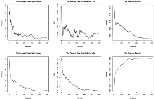
Figure 3: MASS performance graphs in Simulation II. Upper panels are scenario 1 and lower panels scenario 2.

4.3 Simulation study III: Dense $\mathbf{A}$ case

In this simulation we investigated a dense model. We simulated the input data $\mathbf{X}$ (the same size as in Simulation II) from $\mathcal{N}(0,\Sigma)$, where the diagonal elements of $\Sigma$ were 1 and the off-diagonal elements were 0.5. Unlike the sparse case, the elements of the true 5-dimensional $\mathbf{A}_{0}$ were generated from the standard normal distribution. Since the $\mathbf{A}_{0}$ matrix is dense, the columns in $\mathbf{Z}$ will be linear combinations of columns in $\mathbf{X}$. If we use a linear LR model (13) to generate group labels as in Simulation II, the generated group labels will depend on a linear combination of the columns of $\mathbf{Z}$. Therefore, the group labels are actually directly related to a linear combination of all the columns of $\mathbf{X}$, thus, removing the concept of a lower dimensional space. Hence, to ensure the response was a function of the lower dimensional space, we generated the group labels using a nonlinear logistic regression,

$$\Pr(y_{i}=1|Z_{i})=\frac{e^{g(Z_{i})}}{1+e^{g(Z_{i})}},$$ (14)

where $g(Z_{i})=\sin(0.05\pi Z_{i})^{T}\bolds{\beta}$. This guarantees that most $0.05\pi Z_{i}$ values fall into the range of $(-\pi/2,\pi/2)$. Hence, the nonlinearity is produced by that particular part of a sine function.

Since the data scale was moderate and all the variables contain group information, the optimal $p^{*}$ for different methods may be different and not always be $p_{0}$. We reported the average minimal MCR^∗’s and its corresponding $p^{*}$’s for Lars, GLMpath, SIS and PCA, respectively. As to MASS and MFSS, we still fix $p=5$, which is considered a disadvantage for these two but an advantage for other methods. Since $\mathbf{A}_{0}$ is dense, we assigned $\bar{\xi}=0$ to MFSS. Table 6 lists the average MCR^∗ and $p^{*}$’s based on 20 pairs of training and test data. Figure 4 shows the MASS performance graphs. As can be seen, MASS and MFSS are still superior when all the methods use their optimal $p^{*}$’s, with MFSS providing the best results. Figure 5 shows the test MCR values by Lars, GLMpath, SIS and PCA with different $p$’s. These methods all tend to use larger numbers of variables.

Table 6: Average minimum MCR from Simulation III

	LR		SVM
	$\bolds{p^{*}}$	MCR$\bolds{{}^{*}}$	$\bolds{p^{*}}$	MCR$\bolds{{}^{*}}$
Bayes	0.082 (0.002)
FD	—	0.339 (0.006)	—	0.317 (0.007)
Lars	21	0.319 (0.006)	37	0.306 (0.006)
GLMpath	19	0.320 (0.006)	25	0.308 (0.005)
SIS	25	0.321 (0.005)	43	0.305 (0.006)
PCA	32	0.329 (0.005)	35	0.326 (0,006)
MASS($p=5$)		0.271 (0.010)		0.245 (0.008)
MFSS($p=5$)		0.239 (0.008)		0.212 (0.007)

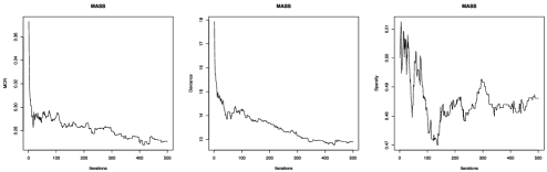
Figure 4: MASS performance graphs in Simulation III with $p=5$.

Figure 5: Average test MCR for all values of $p$ in Simulation III. Upper panels: LR; lower panels: SVM.

4.4 Simulation study IV: Contaminated data

In order to examine the robustness of MASS against outliers, we created a situation where the distributional assumptions were violated. We generated the input data from a multivariate $g$-and-$h$ distribution Field and Genton (2006) with $\mathbf{g}=\mathbf{h}=(0.5,\dots,0.5)^{T}\in\mathbb{R}^{50}$. As with Simulation III, we used Equation (14) to create the group labels, except that here we used $g(Z_{i})=\sin(0.005\pi Z_{i})^{T}\bolds{\beta}$. Since this is a highly skewed and heavy-tailed case, there are many extreme values. Hence, the data domain is rather large. We use $\sin(0.005\pi Z_{i})$ so that most $0.005\pi Z_{i}$ values fall into the range of $(-\pi/2,\pi/2)$. As with Simulation III, only half period of a sine curve is effective.

MASS and MFSS were performed with a fixed $p=5$, while all other methods used their $p^{*}$’s. MFSS was implemented with $\bar{\xi}=0$. The results are listed in Table 7. As with Simulation III, MASS and MFSS with a fixed $p=5$ outperformed other methods with their $p^{*}$’s. All other methods performed poorly on these data. Compared to Simulation III, the performance of MASS and MFSS did not decline as much as other methods. This demonstrates that the proposed method is not very sensitive to outliers.

Table 7: Average minimum MCR from Simulation IV

	LR		SVM
	$\bolds{p^{*}}$	MCR$\bolds{{}^{*}}$	$\bolds{p^{*}}$	MCR$\bolds{{}^{*}}$
Bayes	0.068 (0.002)
FD	—	0.482 (0.006)	—	0.490 (0.007)
Lars	29	0.403 (0.004)	20	0.391 (0.004)
GLMpath	37	0.401 (0.005)	48	0.389 (0.006)
SIS	39	0.410 (0.005)	31	0.392 (0.005)
PCA	35	0.412 (0.005)	31	0.399 (0.005)
MASS($p=5$)		0.294 (0.006)		0.285 (0.007)
MFSS($p=5$)		0.273 (0.005)		0.266 (0.007)

4.5 Simulation study V: Ultra high dimensional data

In this section we simulated an ultra high dimensional situation where $n=100,~{}d=1000$. Thus, a preliminary dimension reduction was needed. Among the $1000$ variables, only 50 contained the group information. These 50 informative variables were generated from a multivariate normal distribution with variance 1 and correlation 0.5. The 950 noise variables were generated from $\mathcal{N}(0,0.5\mathbf{I})$ in order to achieve a reasonable signal-to-noise ratio. Letting $p_{0}=5$, the $\mathbf{Z}_{0}$ was generated from the 50 informative variables through a dense $\mathbf{A}_{0}$, with each element generated from the standard normal distribution. The group labels were still generated by Equation (14).

Figure 6: Average test MCR for all values of $p$ on the first reduced data by Lars in Simulation V. Upper panels: using LR; lower panels: using SVM.

We used the three aforementioned preliminary reduction methods, SIS, PCA and PCA-SIS, to reduce the data into $m=50$ dimensions. Presumably, if the preliminary reduction can extract the $m$ informative variables, MASS and MFSS (with $\bar{\xi}=0$) will perform well. We also implemented Lars and GLMpath on the preliminary reduced data. For Lars and GLMpath, we reported their average test MCR^∗ and $p^{*}$’s, while for MASS and MFSS we still fixed $p=5$. Figure 6 shows the average test MCR from different values of $p$ on the preliminarily reduced data using Lars as the further reduction method. The test MCR for GLMpath looks similar to Lars and thus is not shown. As we can see, no matter what preliminary reduction method is applied, Lars tends to choose larger values of $p^{*}$ than $p_{0}$. However, even with the $p^{*}$’s, the test MCR^∗ are above 0.250. In particular, when PCA and PCA-SIS are applied, MCR^∗ are above 0.320. SIS seems to be a better preliminary reduction method for Lars and GLMpath in this simulation.

The average test MCR, using LR and SVM classifiers, are shown in Table 8. As we can see, all six implementations of MASS and MFSS were statistically significantly better than Lars and GLMpath with their $p^{*}$’s. In particular, SIS-MASS and PCA-SIS-MASS generally provided the best results. It is not surprising that PCA or PCA-SIS as the preliminary reduction methods did not fail, because the signal-to-noise ratio was not large enough in this study. This indicates that the improvement of the classification accuracy by MASS is not only caused by the preliminary reduction but more by the method itself.

In order to further demonstrate that the improvement of the classification accuracy was not due mainly to the preliminary reduction but to the MASS method, we also applied SVM, kNN, NN and RF on the 50-dimensional reduced data without performing any further reduction. The results are shown in Table 9. As can be seen, MASS and MFSS performed extremely well relative to those approaches.

Table 8: Average test MCR (standard errors) in Simulation V

	Classifier	Lars (with $\bolds{p^{*}}$)	GLMpath (with $\bolds{p^{*}}$)	MASS	MFSS
SIS-	LR	0.286 (0.012)	0.288 (0.012)	0.124 (0.007)	0.150 (0.009)
	SVM	0.250 (0.015)	0.253 (0.015)	0.121 (0.008)	0.155 (0.008)
PCA-	LR	0.348 (0.015)	0.347 (0.013)	0.165 (0.011)	0.182 (0.011)
	SVM	0.353 (0.014)	0.356 (0.013)	0.157 (0.011)	0.179 (0.012)
PCA-SIS-	LR	0.337 (0.013)	0.335 (0.012)	0.119 (0.010)	0.125 (0.011)
	SVM	0.325 (0.011)	0.327 (0.010)	0.102 (0.011)	0.119 (0.010)

Table 9: Average test MCR on the 50-dimensional first reduced data using different classifiers

	SVM	kNN	NN	RF
SIS-	0.349 (0.017)	0.356 (0.015)	0.365 (0.016)	0.344 (0.017)
PCA-	0.358 (0.013)	0.377 (0.013)	0.323 (0.013)	0.350 (0.015)
PCA-SIS-	0.359 (0.012)	0.364 (0.014)	0.318 (0.012)	0.351 (0.015)

5 Computational issues

In this section we discuss several issues associated with MASS, including the solution variability, the computational issue and the potential problem of overfitting.

Regarding the randomized nature of MASS, one issue is the variability of the solution, that is, the variability of the selected $\mathbf{A}$ for a fixed training and test pair from different simulation runs. Theoretically, a space is determined by its orthogonal basis. We presume two spaces are the same as long as they have the same basis even though they can be rotated differently. Therefore, $\mathbf{A}$’s can be treated the same if the $\mathbf{Z}$’s they produce have the same principal components (PC). Hence, we examine the first PC of $\mathbf{Z}$’s produced by different simulation runs.

We examine three different cases. The first two are the two scenarios in Simulation II and the third is the fMRI data in Section 3.1. For each of the first two cases, we generate a training data set of 100 observations paired with a test data set of 1000 observations. In each paired data set, we apply MASS 100 times and obtain 100 $\mathbf{Z}$’s. We then extract the first PC for each $\mathbf{Z}$ on the test data and calculate the average absolute pairwise correlations between MASS runs:

$$\overline{|\rho_{\mathrm{PC1}}|}=\frac{1}{4950}\sum_{s<t}|\rho_{s,t}|,$$

where $\rho_{s,t}$ is the correlation of the first PC between the $s$th and the $t$th runs.

For the fMRI data, we fixed the training data (150 observations) and test data (50 observations), and conducted a preliminary reduction using PCA-SIS to reduce the data space to 60 dimensional. The $\overline{|\rho_{\mathrm{PC1}}|}$ was also calculated. In the first two cases, we set $p=5$ and in the third, we set $p=50$.

Table 10 shows $\overline{|\rho_{\mathrm{PC1}}|}$, the proportion of variance that the first PC contains, and the standard errors of test MCR from 100 runs. In all cases, $\overline{|\rho_{\mathrm{PC1}}|}$’s are reasonably high (all above 0.70). Particularly, in the first case, $\overline{|\rho_{\mathrm{PC1}}|}=0.968$, which indicates the first PC accounting for $89\%$ of the data variance, are highly consistent based on 100 simulation runs. PCs containing larger variance are more consistent than PCs with less variance. In addition, the SE for MCR are fairly small for all the cases (e.g., 0.006, 0.007 and 0.005, respectively). All these indicate the solution produced by MASS is fairly stable.

Table 10: Check of solution stability: $\overline{|\rho_{\mathrm{PC1}}|}$’s (standard errors), proportion of variance (standard errors) and standard errors for MCR

	PC1	Variance ($\bolds{\%}$)	SE for MCR
Simulation II (1)	0.968 (0.000)	89% (0.004)	0.006
Simulation II (2)	0.830 (0.001)	74% (0.012)	0.007
fMRI	0.732 (0.002)	42% (0.013)	0.005

We compared MASS on the fMRI data, in terms of both classification accuracy and the computational time, to the SA-Sparse method by Tian, Wilcox and James (2009), which is also a stochastic search procedure. The approach of Tian, Wilcox and James (2009) provides a useful comparison because it also uses a stochastic search but implements the search process using a simulated annealing approach. The code was written in R and run on a Dell Precision workstation (CPU 3.00 GHz; RAM 2.99 GHz, 16.0 GB). We recorded the total CPU time (in seconds) of the R program for both methods. PCA was applied first to reduce the data dimension to $m=80$ and then both methods searched for a $p=30$ dimensional subspace. Table 11 reports the time consumed and the classification accuracy on the test data when both methods use 500 iterations. Both MASS and SA-Sparse took a similar time period to run. The key difference was that MASS converged well before $500$ iterations, while SA-Sparse did not. Hence, the error rate for SA-Sparse was much higher. SA-Sparse took approximately $5000$ iterations to converge, which resulted in an order of magnitude more computational effort. In addition, even when $5000$ iterations were chosen for SA-Sparse, the average test errors were still higher than for the MASS method.

Table 11: Execution time for each run and the average test MCR on fMRI data using SVM

	CPU Time/Run (sec.)	MCR
MASS (500 iterations)	055.3400	0.187 (0.010)
SA-Sparse (500 iterations)	044.7000	0.301 (0.018)
SA-Sparse (5000 iterations)	444.9275	0.237 (0.012)

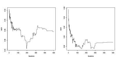
Figure 7: Test MCR paths in Simulation I. Left panel: MFSS with $\lambda=5$; right panel: MFSS with $\lambda=0$.

Since the parameter space for MASS is large ($d\times L$ dimensional), overfitting may be a potential problem. In our nonlinear simulation study, we observed that when the model was very flexible, that is, $\lambda$ was large, MFSS produced poor accuracy. Figure 7 shows the average test MCR paths over 500 iterations in the same setting as Simulation I except with $\lambda_{0}=1$. As is displayed in the left panel of Figure 7, when we assign $\lambda=5$, which is a more flexible model than the true model, the MCR decreases rapidly at the beginning, then it starts increasing dramatically, and it levels off at some point of time. This trend clearly indicates the presence of overfitting. When we used the linear MASS (i.e., assigning $\lambda=0$), which was a less flexible model than the true model, overfitting was less likely to occur. As we can see from the right panel of Figure 7, the MCR decreases rapidly and levels off. In addition, we used a small value for $p$ (the same as the true $p_{0}$). This made the model less flexible. Presumably when $p\gg p_{0}$, overfitting may also become an issue.

6 Discussion

MASS was designed to implement a supervised learning classification method with the flexibility to mimic either a variable selection or a variable combination method. It does this by adaptively adjusting the sparsity of the transformation matrix used to lower the dimensionality of the original data space. We use a stochastic search procedure to address the very high dimensional predictor space. Our simulation results suggest that this approach can provide extremely competitive results relative to a large range of classical and modern classification techniques in both linear and nonlinear cases. We also examined three different preliminary dimension reduction methods which appeared to both increase prediction accuracy as well as improve computational efficiency. MASS seems to converge quickly relative to other stochastic approaches, which makes it feasible to be applied to large data sets. The MASS method for dimensionality reduction could also be generalized to the context of regression where the response is a continuous variable. Further studies are planned for this setting.

Appendix A Proof of Theorem 1

Suppose the theorem is not true. Then for some $\delta>0$ it must be the case that as $n$ and $I$ converge to infinity, $\frac{1}{n}\|\tilde{\mathbf{Z}}_{n}^{(I)}-\mathbf{Z}_{0}\|^{2}>\delta$ happens infinitely often with a probability greater than 0. Without loss of generality, we can assume $\delta<\varepsilon$ where $\varepsilon$ is defined in Assumption 1. But since MASS randomly searches the entire space of $\mathbf{Z}$, as $I\rightarrow\infty$, we are guaranteed at some stage to generate a candidate set of predictors, $\tilde{\mathbf{Z}}_{n}^{(I)}$, such that $\frac{1}{n}\|\tilde{\mathbf{Z}}_{n}^{(I)}-\mathbf{Z}_{0}\|^{2}<\delta<\varepsilon$. The last point to prove is that this candidate set is selected by MASS and does not then get rejected at a later iteration.

By Assumption 1, there exists $\Omega$ with $P(\Omega)=1$ such that for any $\omega\in\Omega$, for all $n>N(\omega)$, $\tilde{\mathbf{Z}}_{n}(\omega)$ is guaranteed to be selected since $\frac{1}{n}\|\tilde{\mathbf{Z}}_{n}(\omega)-\mathbf{Z}_{0}\|^{2}<\varepsilon$. Once $\tilde{\mathbf{Z}}_{n}(\omega)$ is selected, at each future iteration the same set of predictors will be presented to the variable selection method along with other possible candidates. By Assumption 1, the only way that $\tilde{\mathbf{Z}}_{n}(\omega)$ would not be selected at the next iteration would be if an even better set of predictors was generated with squared distance from the true predictors even lower. Hence, as $n$ and $I$ approach infinity, it must be the case that $\frac{1}{n}\|\tilde{\mathbf{Z}}_{n}^{(I)}-\mathbf{Z}_{0}\|^{2}<\delta$. Thus, the theorem is proved.

Appendix B Deduction of nonlinear reduction

We write $f_{j,k}(t)=\mathbf{b}(t)^{T}\theta_{j,k}=b_{1}(t)\theta_{j,k,1}+\cdots+b_{q}(t)\theta_{j,k,q}$, where $\mathbf{b}(t)$ is a NCS basis with $q$ degrees of freedom and $\theta_{j,k}$ is the coefficient vector. We need to generate $\theta_{j,k}$ such that (5) holds. First note that $f^{\prime\prime 2}_{j,k}(t)=\theta^{T}_{j,k}\mathbf{b}^{\prime\prime}(t)\mathbf{b}^{\prime\prime}(t)^{T}\theta_{j,k}$. Then the integral in (5) becomes

$$\int f^{\prime\prime}_{j,k}(t)^{2}\,dt\approx\frac{1}{T}\sum^{T}_{l=1}f^{\prime\prime}_{j,k}(t_{l})^{2}=\theta^{T}_{j,k}\Gamma\theta_{j,k},$$

where $\Gamma=\frac{1}{T}\sum^{T}_{l=1}\mathbf{b}^{\prime\prime}(t_{l})\mathbf{b}^{\prime\prime}(t_{l})^{T}$ and $t_{1},\ldots,t_{T}$ represent a fine grid of time points. Applying the singular value decomposition, we can write $\Gamma=\mathbf{UDU}^{T}$, where $\mathbf{U}$ is orthogonal and $\mathbf{D}=\operatorname{diag}(d_{1},\dots,d_{q-1},0)$. Note the $0$ in the singular value decomposition comes from the slope term (set to zero when you take the second derivative) since there are no intercept terms in the basis function.

We further write

$$\theta^{T}_{j,k}\Gamma\theta_{j,k}=\theta^{T}_{j,k}\mathbf{UDU}^{T}\theta_{j,k}=\theta^{*T}_{j,k}\mathbf{D}\theta^{*}_{j,k}=\theta^{-T}_{j,k}\mathbf{D}^{-}\theta^{-}_{j,k},$$

where $\theta^{*}_{j,k}=\mathbf{U}^{T}\theta_{j,k}$, $\theta^{-}_{j,k}$ is the first $q-1$ elements of $\theta^{*}_{j,k}$, and $\mathbf{D}^{-}=\operatorname{diag}(d_{1},\break\dots,d_{q-1})$. Hence, we need to constrain $\theta^{-T}_{j,k}\mathbf{D}^{-}\theta^{-}_{j,k}\leq\lambda$. This is easily achieved by first generating the $\theta_{j,k}$’s as described in (7) and (8), and computing the corresponding $\theta^{-}_{j,k}$. We then reset $\theta^{-}_{j,k}$ via

$$\theta^{-}_{j,k}\leftarrow\theta^{-}_{j,k}\sqrt{\frac{\lambda}{\theta^{-T}_{j,k}\mathbf{D}^{-}\theta^{-}_{j,k}}}$$

and let $\theta_{jk}={\bf U}\theta^{*}_{j,k}={\bf U}(\theta^{-}_{j,k},\theta^{*}_{j,k,q})^{T}$.

We write

$$f_{j,k}(t)=\mathbf{b}(t)^{T}\mathbf{U}(\theta^{-}_{j,k},\theta^{*}_{j,k,q})^{T}=(\mathbf{b}(t)^{T}\mathbf{U})\theta^{-}_{j,k}+(\mathbf{b}(t)^{T}\mathbf{U})_{q}\theta^{*}_{j,k,q}.$$

In particular, if $\lambda=0$, all elements in $\theta^{-}_{j,k}$ are zero, in which case the integral is also zero and a linear fit is produced, that is, $f_{j,k}(t)=(\mathbf{b}(t)^{T}\mathbf{U})_{q}\theta^{*}_{j,k,q}$.

Since $\theta^{*}_{j,k,q}$ indicates the slope term, standardizing $f_{j,k}$ is equivalent to standardize all the $\theta^{*}_{j,k,q}$’s. We let

$$f^{*}_{j,k}(t)=(\mathbf{b}(t)^{T}\mathbf{U})_{q}\theta^{*}_{j,k,q}=\upsilon t\theta^{*}_{j,k,q},$$

where $\upsilon^{2}=\frac{1}{t}(\mathbf{b}(t)^{T}\mathbf{U})_{q}$. Standardizing $f_{j,k}$ involves setting

$$\sum^{d}_{k=1}\upsilon^{2}\theta^{*2}_{j,k,q}=1.$$

Hence, we reset $\theta^{*}_{j,k,q}$ by

$$\theta^{*}_{j,k,q}\leftarrow\frac{\theta^{*}_{j,k,q}}{\upsilon_{k}\sqrt{\sum^{d}_{k=1}\upsilon^{2}\theta^{*2}_{j,k,q}}}.$$

This approach ensures that (5) holds for all candidate functions.

References

- Candes and Tao (2007) Candes, E. and Tao, T. (2007). The dantzig selector: Statistical estimation when is much larger than (with discussion). Ann. Statist. 35 2313–2351. \MR2382644
- Efron et al. (2004) Efron, B., Hastie, T., Johnstone, I. and Tibshirani, R. (2004). Least angle regression. Ann. Statist. 32 407–451. \MR2060166
- Fan and Fan (2008) Fan, J. and Fan, Y. (2008). High dimensional classification using features annealed independence rules. Ann. Statist. 36 2605–2637. \MR2485009
- Fan and Li (2001) Fan, J. and Li, R. (2001). Variable selection via nonconcave penalized likelihood and its oracle properties. J. Amer. Statist. Assoc. 96 1348–1360. \MR1946581
- Fan and Lv (2008) Fan, J. and Lv, J. (2008). Sure independence screening for ultra-high dimensional feature space. J. Roy. Statist. Soc. Ser. B 70 849–911.
- Field and Genton (2006) Field, C. and Genton, M. G. (2006). The multivariate -and- distribution. Technometrics 48 104–111. \MR2236532
- George and McCulloch (1993) George, E. I. and McCulloch, R. E. (1993). Variable selection via gibbs sampling. J. Amer. Statist. Assoc. 88 881–889.
- George and McCulloch (1997) George, E. I. and McCulloch, R. E. (1997). Approaches for bayesian variable selection. Statistica Sinica 7 339–373.
- Golub et al. (1999) Golub, T., Slonim, D., Tamayo, P., Huard, C., Gaasenbeek, M., Mesirov, J., Coller, H., Loh, M., Downing, J., Caligiuri, M., Bloomfield, C. and Lander, E. (1999). Molecular classification of cancer: Class discovery and class prediction by gene expression monitoring. Science 286 531–537.
- Gosavi (2003) Gosavi, A. (2003). Simulation-Based Optimization: Parametric Optimization Techniques and Reinforcement Learning. Kluwer, Boston. \MR1996863
- Knight and Fu (2000) Knight, L. and Fu, W. (2000). Asymptotics for lasso-type estimators. Ann. Statist. 28 1356–1378. \MR1805787
- Liberti and Kucherenko (2005) Liberti, L. and Kucherenko, S. (2005). Comparison of deterministic and stochastic approaches to global optimization. Int. Trans. Oper. Res. 12 263–285. \MR2141235
- Mitchell and Beauchamp (1988) Mitchell, T. J. and Beauchamp, J. J. (1988). Bayesian variable selection in linear regression (with discussion). J. Amer. Statist. Assoc. 83 1023–1036. \MR0997578
- Park and Hastie (2007) Park, M.-Y. and Hastie, T. (2007). An regularization-path algorithm for generalized linear models. J. Roy. Statist. Soc. Ser. B 69 659–677. \MR2370074
- Radchenko and James (2008) Radchenko, P. and James, G. (2008). Variable inclusion and shrinkage algorithms. J. Amer. Statist. Assoc. 103 1304–1315. \MR2462899
- Radchenko and James (2009) Radchenko, P. and James, G. (2009). Forward-lasso with adaptive shrinkage. Under review.
- Reinsch (1967) Reinsch, C. (1967). Smoothing by spline functions. Numer. Math. 10 177–183. \MR0295532
- Roweis and Saul (2000) Roweis, S. and Saul, L. (2000). Nonlinear dimensionality reduction by locally linear embedding. Science 290 2323–2326.
- Tenenbaum, de Silva and Langford (2000) Tenenbaum, J., de Silva, V. and Langford, J. (2000). A global geometric framework for nonlinear dimensionality reduction. Science 290 2319–2323.
- Tian, Wilcox and James (2009) Tian, T. S., Wilcox, R. R. and James, G. M. (2009). Data reduction in classification: A simulated annealing based projection method. Under review.
- Tibshirani (1996) Tibshirani, R. (1996). Regression shrinkage and selection via the lasso. J. Roy. Statist. Soc. Ser. B 58 267–288. \MR1379242
- Tibshirani et at. (2002) Tibshirani, R., Hastie, T., Narasimhan, B. and Chu, G. (2002). Diagnosis of multiple cancer types by shrunken centroids of gene expression. Proc. Natl. Acad. Sci. USA 99 6567–6572.
- Tsybakov and van de Geer (2005) Tsybakov, A. and van de Geer, S. (2005). Square root penalty: Adaptation to the margin in classification and in edge estimation. Ann. Statist. 33 1203–1224. \MR2195633
- Zou and Hastie (2005) Zou, H. and Hastie, T. (2005). Regularization and variable selection via the elastic net. J. Roy. Statist. Soc. Ser. B 67 301–320. \MR2137327