On the Critical Behavior, the Connection Problem

and the Elliptic Representation

of a Painlevé 6 Equation (Spring 2001)

Davide Guzzetti, May 2001

  Abstract.

In this paper we find a class of solutions of the sixth Painlevé equation appearing in the theory of WDVV equations. This class covers almost all the monodromy data associated to the equation, except one point in the space of the data. We describe the critical behavior close to the critical points in terms of two parameters and we find the relation among the parameters at the different critical points (connection problem). We also study the critical behavior of Painlevé transcendents in the Elliptic representation.

KEY WORDS: Painlevé equation, Elliptic function, isomonodromic deformation, Fuchsian system, connection problem, monodromy.

AMS CLASSIFICATION: 34M55

1 Introduction

This paper was completed in May 2001, at RIMS, Kyoto University. It is published in J. Math. Phys. Anal. Geom. 4: 293-377 (2001). I put it on the archive with 9 years delay, for completeness sake. In the meanwhile, there have been several progresses. Nevertheless, this paper contains an important detailed analysis which has not been repeated in subsequent papers.

This work is devoted to the study of the critical behavior of the solutions of a Painlevé 6 equation given by a particular choice of the four parameters $\alpha$, $\beta$, $\gamma$ $\delta$ of the equation (the notations are the standard ones, see [18]):

$$\alpha={(2\mu-1)^{2}\over 2},~{}~{}~{}\beta=\gamma=0,~{}~{}~{}\delta={1\over 2},~{}~{}~{}~{}~{}\mu\in{\bf C}.$$

The equation is

$${d^{2}y\over dx^{2}}={1\over 2}\left[{1\over y}+{1\over y-1}+{1\over y-x}\right]\left({dy\over dx}\right)^{2}-\left[{1\over x}+{1\over x-1}+{1\over y-x}\right]{dy\over dx}$$

$$+{1\over 2}{y(y-1)(y-x)\over x^{2}(x-1)^{2}}\left[(2\mu-1)^{2}+{x(x-1)\over(y-x)^{2}}\right],~{}~{}~{}~{}~{}\mu\in{\bf C}.$$ (1)

Such an equation will be denoted $PVI_{\mu}$ in the paper. The motivation of our work is that (1) is equivalent to the WDVV equations of associativity in 2-D topological field theory introduced by Witten [39], Dijkgraaf, Verlinde E., Verelinde H. [6]. Such an equivalence is discussed in [9] and it is a consequence of the theory of Frobenius manifolds. Frobenius manifolds are the geometrical setting for the WDVV equations and were introduced by Dubrovin in [7]. They are an important object in many branches of mathematics like singularity theory and reflection groups [34] [35] [12] [9], algebraic and enumerative geometry [24] [26].

The six classical Painlevé equations were discovered by Painlevé [31] and Gambier [15], who classified all the second order ordinary differential equations of the type

$${d^{2}y\over dx^{2}}={\cal R}\left(x,y,{dy\over dx}\right)$$

where ${\cal R}$ is rational in ${dy\over dx}$, $x$ and $y$. The Painlevé equations satisfy the Painlevé property of absence of movable branch points and essential singularities. These singularities will be called critical points; for $PVI_{\mu}$ they are 0,1,$\infty$. The behavior of a solution close to a critical point is called critical behavior. The general solution of the sixth Painlevé equation can be analytically continued to a meromorphic function on the universal covering of ${\bf P}^{1}\backslash\{0,1,\infty\}$. For generic values of the integration constants and of the parameters in the equation, it can not be expressed via elementary or classical transcendental functions. For this reason, it is called a Painlevé transcendent.

The critical behavior for a class of solutions to the Painlevé 6 equation was found by Jimbo in [20] for the general Painlevé equation with generic values of $\alpha$, $\beta$, $\gamma$ $\delta$ (we refer to [20] for a precise definition of generic). A transcendent in this class has behavior:

$$y(x)=a^{(0)}x^{1-\sigma^{(0)}}(1+O(|x|^{\delta})),~{}~{}~{}~{}x\to 0,$$ (2)

$$y(x)=1-a^{(1)}(1-x)^{1-\sigma^{(1)}}(1+O(|1-x|^{\delta})),~{}~{}~{}~{}x\to 1,$$ (3)

$$y(x)=a^{(\infty)}x^{-\sigma^{(\infty)}}(1+O(|x|^{-\delta})),~{}~{}~{}~{}x\to\infty,$$ (4)

where $\delta$ is a small positive number, $a^{(i)}$ and $\sigma^{(i)}$ are complex numbers such that $a^{(i)}\neq 0$ and

$$0\leq\Re\sigma^{(i)}<1.$$ (5)

We remark that $x$ converges to the critical points inside a sector with vertex on the corresponding critical point.

The connection problem, i.e. the problem of finding the relation among the three pairs $(\sigma^{(i)},a^{(i)})$, $i=0,1,\infty$, was solved by Jimbo in [20] for the above class of transcendents using the isomonodromy deformations theory. He considered a fuchsian system

$${dY\over dz}=\left[{A_{0}(x)\over z}+{A_{x}(x)\over z-x}+{A_{1}(x)\over z-1}\right]Y$$

such that the $2\times 2$ matrices $A_{i}(x)$ ($i=0,x,1$ are labels) satisfy Schlesinger equations. This ensures that the dependence on $x$ is isomonodromic, according to the isomonodromic deformation theory developed in [21]. Moreover, for a special choice of the matrices, the Schlesinger equations are equivalent to the sixth Painlevé equation, as it is explained in [22]. In particular, the local behaviors (2), (3), (4) were obtained using a result on the asymptotic behavior of a class of solutions of Schlesinger equations proved by Sato, Miwa, Jimbo in [33]. The connection problem was solved because the parameters $\sigma^{(i)}$, $a^{(i)}$ were expressed as functions of the monodromy data of the fuchsian system. For studies on the asymptotic behavior of the coefficients of Fuchsian systems and Schlesinger equations see also [5].

Later, Dubrovin and Mazzocco [13] applied Jimbo’s procedure to $PVI_{\mu}$, with the restriction that $2\mu\not\in{\bf Z}$. We remark that this case was not studied by Jimbo, being a non-generic case. Dubrovin and Mazzocco obtained a class of transcendents with behaviors (2), (3), (4) (again, $x$ converges to a critical point inside a sector) and restriction (5). They also solved the connection problem.

In the case of $PVI_{\mu}$, the monodromy data of the Fuchsian system, to be introduced later, turn out to be expressed in terms of a triple of complex numbers $(x_{0},x_{1},x_{\infty})$. The two integration constants in $y(x)$ and the parameter $\mu$ are contained in the triple. The following relation holds:

$$x_{0}^{2}+x_{1}^{2}+x_{\infty}^{2}-x_{0}x_{1}x_{\infty}=4\sin^{2}(\pi\mu).$$ (6)

There exists a one-to-one correspondence between triples (define up to the change of two signs) and branches of the Painlevé transcendents. ¹ In other words, any branch $y(x)$ is parameterized by a triple:

$$y(x)=y(x;x_{0},x_{1},x_{\infty}).$$

As it is proved in [13], the transcendents (2), (3), (4) are parameterized by a triple according to the formulae

$$x_{i}^{2}=4\sin^{2}\left({\pi\over 2}\sigma^{(i)}\right),~{}~{}~{}i=0,1,\infty,~{}~{}~{}~{}~{}~{}~{}~{}0\leq\Re\sigma^{(i)}<1.$$

A more complicated expression gives $a^{(i)}=a^{(i)}(x_{0},x_{1},x_{\infty})$ in [13]. We recall that a branch is defined by the choice of branch cuts, like $|\arg(x)|<\pi$, $|\arg(1-x)|<\pi$. The analytic continuation of a branch when $x$ crosses the cuts is obtained by an action of the braid group on the triple. This is explained in [13] and in section 6.

As we mentioned above, it is very important to concentrate on $PVI_{\mu}$ due to its equivalence to WDVV equations in 2-D topological field theory, and due to its central role in the construction of three-dimensional Frobenius manifolds. It is known [9] that the structure of a local chart of a Frobenius manifold can in principle be constructed from a set of monodromy data. To any manifold a $PVI_{\mu}$ equation is associated and the monodromy data of the local chart are contained in $\mu$ and in the triple $(x_{0},x_{1},x_{\infty})$ of a Painlevé transcendent. The mentioned action of the braid group, which gives the analytic continuation of the transcendent, allows to pass from one local chart to another.

The local structure of a Frobenius manifold is explicitly constructed in [17] starting from the Painlevé transcendents. In [17] it is shown that in order to obtain a local chart from its monodromy data we need to know the critical behavior of the corresponding transcendent in terms of the triple $(x_{0},x_{1},x_{\infty})$ (note that this is equivalent to solving the connection problem).

Recently, Frobenius manifolds have become important in enumerative geometry and quantum cohomology [24], [26]. As it is shown in [17], it is possible to compute Gromov-Witten invariants for the quantum cohomology of the two-dimensional projective space starting from a special $PVI_{\mu}$, with $\mu=-1$. In this case the triple is $(x_{0},x_{1},x_{\infty})=(3,3,3)$, as it is proved in [10] and [16]. Due to the restriction $0\leq\Re\sigma^{(i)}<1$, the formulae for the critical behavior and the connection problem obtained by Dubrovin-Mazzocco do not apply if at least one $x_{i}$ ($i=0,1,\infty$) is real and $|x_{i}|\geq 2$. Thus, they do not apply in the case of quantum cohomology, because $x_{i}=3$ and $\Re\sigma^{(i)}=1$.

Therefore, the motivation of our paper becomes clear: in the attempt to extend the results of [13] to the case of quantum cohomology, we actually extended them to almost all monodromy data, namely we found the critical behavior and we solved the connection problem for all the triples satisfying

$$x_{i}\neq\pm 2~{}~{}\Longrightarrow~{}~{}\sigma^{(i)}\neq 1,~{}~{}~{}~{}i=0,1,\infty.$$

In order to do this, we extended Jimbo and Dubrovin-Mazzocco’s method and we analyzed the elliptic representation of the Painlevé 6 equation.

1.1 Our results

We observe that the branch $y(x;x_{0},x_{1},x_{\infty})$ has analytic continuation on the universal covering of ${\bf P}^{1}\backslash\{0,1,\infty\}$. We still denote this continuation by $y(x;x_{0},x_{1},x_{\infty})$, where $x$ is now a point in the universal covering. Therefore:

There is a one to one correspondence between triples of monodromy data $(x_{0},x_{1},x_{\infty})$ (defined up to the change of two signs) and Painlevé transcendents, namely $y(x)=y(x;x_{0},x_{1},x_{\infty})$, $x\in\widetilde{{\bf P}^{1}\backslash}\{0,1,\infty\}$

We mentioned that if we fix a branch, namely if we choose branch cuts like $|\arg x|<\pi$, $|\arg(1-x)|<\pi$, then the branch of $y(x;x_{0},x_{1},x_{\infty})$ has analytic continuation $y(x;x_{0}^{\prime},x_{1}^{\prime},x_{\infty}^{\prime})$ in the cut plane, where $(x_{0}^{\prime},x_{1}^{\prime},x_{\infty}^{\prime})$ is obtained from $(x_{0},x_{1},x_{\infty})$ by an action of the braid group (see section 6 for details).

We obtained the following results 1)A transcendent $y(x;x_{0},x_{1},x_{\infty})$ such that $|x_{i}|\neq 2$ has behaviors (2), (3), (4) in suitable domains, to be defined below, contained in $\widetilde{{\bf C}\backslash\{0\}}$, $\widetilde{{\bf C}\backslash\{1\}}$, $\widetilde{{\bf P}^{1}\backslash\{\infty\}}$ respectively. The exponent are restricted by the condition $\sigma^{(i)}\not\in(-\infty,0)\cup[1,+\infty)$, which extends (5).

2) The parameters $\sigma^{(i)}$, $a^{(i)}$ are computed as functions of $(x_{0},x_{1},x_{\infty})$, and vice versa, by explicit formulae which extend those of [13]

3) If we enlarge the domains where (2), (3), (4) hold, the behavior of $y(x;x_{0},x_{1},x_{\infty})$ becomes oscillatory. The movable poles of the transcendent lie outside the enlarged domains. In proving this, we investigated the elliptic representation of the transcendent, providing a general result stated in Theorem 3 below.

We state result 1) in more detail. Let $\sigma^{(0)}$ be a complex number such that $\sigma^{(0)}\not\in(-\infty,0)\cup[1,+\infty)$. We introduce additional parameters $\theta_{1}$, $\theta_{2}\in{\bf R}$, $0<\tilde{\sigma}<1$ to define a domain

$$D(\epsilon;\sigma^{(0)};\theta_{1},\theta_{2},\tilde{\sigma}):=\{{x}\in\widetilde{{\bf C}_{0}}\hbox{ s.t. }|x|<\epsilon,~{}~{}e^{-\theta_{1}\Im\sigma^{(0)}}|x|^{\tilde{\sigma}}\leq|{x}^{\sigma^{(0)}}|\leq e^{-\theta_{2}\Im\sigma^{(0)}},~{}~{}~{}0<\tilde{\sigma}<1\},$$

which can can be rewritten as

$$|x|<\epsilon,~{}~{}~{}~{}~{}\Re\sigma^{(0)}\log|x|+\theta_{2}\Im\sigma^{(0)}\leq\Im\sigma^{(0)}\arg(x)\leq(\Re\sigma^{(0)}-\tilde{\sigma})\log|x|+\theta_{1}\Im\sigma^{(0)}$$

For real $\sigma^{(0)}$ the domain is more simply defined as

$$D(\sigma^{(0)};\epsilon):=\{{x}\in\widetilde{{\bf C}_{0}}\hbox{ s.t. }|x|<\epsilon\},~{}~{}~{}~{}~{}\hbox{ for }0\leq\sigma^{(0)}<1$$ (7)

For semplicity, we study the critical behavior of the transcendent for $x\to 0$ along the family of path defined below. Such paths start at some point $x_{0}$ belonging to the domain. If $\Im\sigma=0$ any regular path will be allowed. If $\Im\sigma\neq 0$, we considered the family

$$|x|\leq|x_{0}|<\epsilon,~{}~{}~{}~{}\arg x=\arg x_{0}+{\Re\sigma^{(0)}-\Sigma\over\Im\sigma^{(0)}}\ln{|x|\over|x_{0}|},~{}~{}~{}~{}~{}0\leq\Sigma\leq\tilde{\sigma}$$ (8)

The condition $0\leq\Sigma\leq\tilde{\sigma}$ ensures that the paths remain in the domain as $x\to 0$. In general, these paths are spirals.

Theorem 1: Let $\mu\neq 0$. For any $\sigma^{(0)}\not\in(-\infty,0)\cup[1,+\infty)$, for any $a^{(0)}\in{\bf C}$, $a^{(0)}\neq 0$, for any $\theta_{1},\theta_{2}\in{\bf R}$ and for any $0<\tilde{\sigma}<1$, there exists a sufficiently small positive $\epsilon$ and a small positive number $\delta$ such that the equation (1) has a solution

$$y(x;\sigma^{(0)},a^{(0)})=a(x)~{}x^{1-\sigma^{(0)}}\left(1+O(|x|^{\delta})\right),~{}~{}~{}~{}0<\delta<1,$$ (9)

as $x\to 0$ along (8) in the domain $D(\epsilon;\sigma^{(0)};\theta_{1},\theta_{2},\tilde{\sigma})$ defined for non-real $\sigma^{(0)}$, or along any regular path in $D(\epsilon;\sigma^{(0)})$ defined for real $0\leq\sigma^{(0)}<1$. The amplitude $a(x)$ is

$$a(x):=a^{(0)},~{}~{}~{}~{}\hbox{ for $0<\Sigma\leq\tilde{\sigma}$, or for real $\sigma^{(0)}$ }$$

$$a({x}):=a^{(0)}~{}\left(1+{1\over 2a^{(0)}}~{}|x_{0}^{\sigma^{(0)}}|e^{i\alpha({x})}+{1\over 16[a^{(0)}]^{2}}~{}|x_{0}^{\sigma^{(0)}}|^{2}e^{2i\alpha({x})}\right)=O(1),~{}~{}~{}~{}\hbox{ for $\Sigma=0$}$$ (10)

where we have used the notaion $\alpha(x)$ to denote the real phase of $x^{\sigma^{(0)}}=|x^{\sigma^{(0)}}|~{}e^{i\alpha(x)}\equiv|x_{0}^{\sigma^{(0)}}|~{}e^{i\alpha(x)}$, when $\Sigma=0$.

Note that in the case (10) we can rewrite

$$y({x};\sigma^{(0)},a^{(0)})=\sin^{2}\left({i\sigma^{(0)}\over 2}\ln x-{i\over 2}\ln(4a^{(0)})-{\pi\over 2}\right)~{}x~{}(1+O(|x|^{\delta}))$$ (11)

For brevity, we will sometime denote the domain by $D(\sigma^{(0)})$. The condition $\mu\neq 0$ is not restrictive because $PVI_{\mu=0}$ coincides with $PVI_{\mu=1}$.

From Theorem 1 and the symmetries of (1), we prove the existence of solutions with the following local behaviors

$$y(x,\sigma^{(1)},a^{(1)})=1-a^{(1)}(1-x)^{1-\sigma^{(1)}}(1+O(|1-x|^{\delta}))~{}~{}~{}~{}x\to 1$$

$$a^{(1)}\neq 0,~{}~{}~{}~{}\sigma^{(1)}\not\in(-\infty,0)\cup[1,+\infty)$$

and

$$y(x;\sigma^{(\infty)},a^{(\infty)})=a^{(\infty)}{x}^{\sigma^{(\infty)}}\left(1+O({1\over|x|^{\delta}})\right)~{}~{}~{}~{}~{}x\to\infty$$

$$a^{(\infty)}\neq 0,~{}~{}~{}~{}\sigma^{(\infty)}\not\in(-\infty,0)\cup[1,+\infty)$$

in domains $D(\sigma^{(1)})$, $D(\sigma^{(\infty)})$ given by (50), (47) respectively.

The critical behaviors above coincide with (2), (3) and (4) for $0\leq\Re\sigma^{(i)}<1$, $i=0,1,\infty$. But our result is more general because it extends the range of $\sigma^{(i)}$ to $\Re\sigma^{(i)}<0$ and $\Re\sigma^{(i)}\geq 1$. For this larger range, $x$ may tend to $x=i$ ($i=0,1,\infty$) along a spiral, according to the shape of $D(\sigma^{(i)})$. For more comments see sections 3 and 7.

Result 2) is stated in the theorem below – where we write $\sigma,a$ instead of $\sigma^{(0)},a^{(0)}$ – and in its comment.

Theorem 2: Let $\mu$ be any non zero complex number.

The transcendent $y(x;\sigma,a)$ of Theorem 1, defined for $\sigma\not\in(-\infty,0)\cup[1,+\infty)$ and $a\neq 0$, is the representation of a transcendent $y(x;x_{0},x_{1},x_{\infty})$ in $D(\sigma)$. The triple ($x_{0},x_{1},x_{\infty}$) is uniquely determined (up to the change of two signs) by the following formulae: i) $\sigma\neq 0,\pm 2\mu+2m$ for any $m\in{\bf Z}$.

$$\left\{\matrix{x_{0}=2\sin({\pi\over 2}\sigma)\cr\cr x_{1}=i\left({1\over f(\sigma,\mu)G(\sigma,\mu)}~{}\sqrt{a}-G(\sigma,\mu)~{}{1\over\sqrt{a}}\right)\cr\cr x_{\infty}={1\over f(\sigma,\mu)G(\sigma,\mu)e^{-{i\pi\sigma\over 2}}}~{}\sqrt{a}+G(\sigma,\mu)e^{-i{\pi\sigma\over 2}}~{}{1\over\sqrt{a}}\cr}\right.$$

where

$$f(\sigma,\mu)={2\cos^{2}({\pi\over 2}\sigma)\over\cos(\pi\sigma)-\cos(2\pi\mu)},~{}~{}~{}~{}~{}~{}G(\sigma,\mu)={1\over 2}{4^{\sigma}\Gamma({\sigma+1\over 2})^{2}\over\Gamma(1-\mu+{\sigma\over 2})\Gamma(\mu+{\sigma\over 2})}$$

Any sign of $\sqrt{a}$ is good (changing the sign of $\sqrt{a}$ is equivalent to changing the sign of both $x_{1}$, $x_{\infty}$). ii) $\sigma=0$

$$\left\{\matrix{x_{0}=0\cr\cr x_{1}^{2}=2\sin(\pi\mu)~{}\sqrt{1-a}\cr\cr x_{\infty}^{2}=2\sin(\pi\mu)~{}\sqrt{a}\cr}\right.$$

We can take any sign of the square roots

iii) $\sigma=\pm 2\mu+2m$.

iii1) $\sigma=2\mu+2m$, $m=0,1,2,...$

$$\left\{\matrix{x_{0}=2\sin(\pi\mu)\cr\cr x_{1}=-{i\over 2}{16^{\mu+m}\Gamma(\mu+m+{1\over 2})^{2}\over\Gamma(m+1)\Gamma(2\mu+m)}~{}{1\over\sqrt{a}}\cr\cr x_{\infty}=i~{}x_{1}~{}e^{-i\pi\mu}\cr}\right.$$

iii2) $\sigma=2\mu+2m$, $m=-1,-2,-3,...$

$$\left\{\matrix{x_{0}=2\sin(\pi\mu)\cr\cr x_{1}=2i{\pi^{2}\over\cos^{2}(\pi\mu)}{1\over 16^{\mu+m}\Gamma(\mu+m+{1\over 2})^{2}\Gamma(-2\mu-m+1)\Gamma(-m)}~{}\sqrt{a}\cr\cr x_{\infty}=-ix_{1}e^{i\pi\mu}}\right.$$

iii3) $\sigma=-2\mu+2m$, $m=1,2,3,...$

$$\left\{\matrix{x_{0}=-2\sin(\pi\mu)\cr\cr x_{1}=-{i\over 2}{16^{-\mu+m}\Gamma(-\mu+m+{1\over 2})^{2}\over\Gamma(m-2\mu+1)\Gamma(m)}~{}{1\over\sqrt{a}}\cr\cr x_{\infty}=ix_{1}e^{i\pi\mu}\cr}\right.$$

iii4) $\sigma=-2\mu+2m$, $m=0,-1,-2,-3,...$

$$\left\{\matrix{x_{0}=-2\sin(\pi\mu)\cr\cr x_{1}=2i{\pi^{2}\over\cos^{2}(\pi\mu)}{1\over 16^{-\mu+m}\Gamma(-\mu+m+{1\over 2})^{2}\Gamma(2\mu-m)\Gamma(1-m)}~{}\sqrt{a}\cr\cr x_{\infty}=-ix_{1}e^{-i\pi\mu}\cr}\right.$$

In all the above formulae the relation $x_{0}^{2}+x_{1}^{2}+x_{\infty}^{2}-x_{0}x_{1}x_{\infty}=4\sin^{2}(\pi\mu)$ is automatically satisfied. Note that $\sigma\neq 1$ implies $x_{0}\neq\pm 2$. Changes of two signs in the triple of the formulae above are allowed.

Conversely, a transcendent $y(x;x_{0},~{}x_{1},~{}x_{\infty})$, such that $x_{0}^{2}+x_{1}^{2}+x_{\infty}^{2}-x_{0}x_{1}x_{\infty}=4\sin^{2}(\pi\mu)$, $x_{i}\neq\pm 2$, has representation $y(x;\sigma,a)$ in $D(\sigma)$ of Theorem 1 with parameters $\sigma$ and $a$ obtained as follows:

I) Generic case

$$\cos(\pi\sigma)=1-{x_{0}^{2}\over 2}$$

$$a={iG(\sigma,\mu)^{2}\over 2\sin(\pi\sigma)}\Bigl{[}2(1+e^{-i\pi\sigma})-f(x_{0},x_{1},x_{\infty})(x_{\infty}^{2}+e^{-i\pi\sigma}x_{1}^{2})\Bigr{]}~{}f(x_{0},x_{1},x_{\infty})$$

where

$$f(x_{0},x_{1},x_{\infty}):=f(\sigma(x_{0}),\mu)={4-x_{0}^{2}\over 2-x_{0}^{2}-2\cos(2\pi\mu)}={4-x_{0}^{2}\over x_{1}^{2}+x_{\infty}^{2}-x_{0}x_{1}x_{\infty}}.$$

$\sigma$ is determined up to the ambiguity $\sigma\mapsto\pm\sigma+2n$, $n\in{\bf Z}$ [see Remark below]. If $\sigma$ is real we can only choose the solution satisfying $0\leq\sigma<1$. Any solution $\sigma$ of the first equation must satisfy the additional restriction $\sigma\neq\pm 2\mu+2m$ for any $m\in{\bf Z}$, otherwise we encounter the singularities in $G(\sigma,\mu)$ and in $f(\sigma,\mu)$.

II) $x_{0}=0$.

$$\sigma=0,$$

$$a={x_{\infty}^{2}\over x_{1}^{2}+x_{\infty}^{2}}.$$

provided that $x_{1}\neq 0$ and $x_{\infty}\neq 0$, namely $\mu\not\in{\bf Z}$. III) $x_{0}^{2}=4\sin^{2}(\pi\mu)$. Then (6) implies $x_{\infty}^{2}=-x_{1}^{2}~{}\exp(\pm 2\pi i\mu)$ . Four cases which yield the values of $\sigma$ non included in I) and II) must be considered

III1) If $x_{\infty}^{2}=-x_{1}^{2}e^{-2\pi i\mu}$ then

$$\sigma=2\mu+2m,~{}~{}~{}~{}m=0,1,2,...$$

$$a=-{1\over 4x_{1}^{2}}{16^{2\mu+2m}\Gamma(\mu+m+{1\over 2})^{4}\over\Gamma(m+1)^{2}\Gamma(2\mu+m)^{2}}$$

III2) If $x_{\infty}^{2}=-x_{1}^{2}e^{2\pi i\mu}$ then

$$\sigma=2\mu+2m,~{}~{}~{}~{}m=-1,-2,-3,...$$

$$a=-{\cos^{4}(\pi\mu)\over 4\pi^{4}}16^{2\mu+2m}\Gamma(\mu+m+{1\over 2})^{4}\Gamma(-2\mu-m+1)^{2}\Gamma(-m)^{2}~{}x_{1}^{2}$$

III3)If $x_{\infty}^{2}=-x_{1}^{2}e^{2\pi i\mu}$ then

$$\sigma=-2\mu+2m,~{}~{}~{}~{}m=1,2,3,...$$

$$a=-{1\over 4x_{1}^{2}}{16^{-2\mu+2m}\Gamma(-\mu+m+{1\over 2})^{4}\over\Gamma(m-2\mu+1)^{2}\Gamma(m)^{2}}$$

III4) If $x_{\infty}^{2}=-x_{1}^{2}e^{-2\pi i\mu}$ then

$$\sigma=-2\mu+2m,~{}~{}~{}~{}m=0,-1,-2,-3,...$$

$$a=-{\cos^{4}(\pi\mu)\over 4\pi^{4}}16^{-2\mu+2m}\Gamma(-\mu+m+{1\over 2})^{4}\Gamma(2\mu-m)^{2}\Gamma(1-m)^{2}~{}x_{1}^{2}$$

Let us restore the notation $\sigma^{(0)},a^{(0)}$. At $x=1,\infty$ the exponents $\sigma^{(i)}$, $i=1,\infty$ are given by $\cos(\pi\sigma^{(i)})=1-{x_{i}^{2}\over 2}$ and the coefficients $a^{(1)}$, $a^{(\infty)}$ are obtained from the formula of $a=a^{(0)}$ of Theorem 2, provided that we do the substitutions $(x_{0},x_{1},x_{\infty})\mapsto(x_{1},x_{0},x_{0}x_{1}-x_{\infty})$, $\sigma^{(0)}\mapsto\sigma^{(1)}$ and $(x_{0},x_{1},x_{\infty})\mapsto(x_{\infty},-x_{1},x_{0}-x_{1}x_{\infty})$, $\sigma^{(0)}\mapsto\sigma^{(\infty)}$ respectively.

This also solves the connection problem for the transcendents $y(x;\sigma^{(i)},a^{(i)})$, because we are able to compute $(\sigma^{(i)},a^{(i)})$ for $i=0,1,\infty$ in terms of a fixed triple $(x_{0},x_{1},x_{\infty})$.

Remark : Let $(x_{0},x_{1},x_{\infty})$ be given and let us compute $\sigma$ and $a$ by the formulae of Theorem 2. The equation

$$\cos(\pi\sigma)=1-{x_{0}^{2}\over 2}$$ (12)

does not determine $\sigma$ uniquely. We can choose $\sigma$ such that

$$0\leq\Re\sigma\leq 1.$$

This convention will be assumed in the paper. Therefore, all the solutions of (12) are

$$\pm\sigma+2n,~{}~{}~{}~{}n\in{\bf Z}.$$

If $\sigma$ is real, we can only choose $0\leq\sigma<1$. With this convention, there is a one to one correspondence between $(\sigma,a)$ and (a class of equivalence, defined by the change of two signs, of) an admissible triple $(x_{0},x_{1},x_{\infty})$.

We observe that $\sigma=\sigma(x_{0})$ and $a=a(\sigma;x_{0},x_{1},x_{\infty})$; namely, the transformation $\sigma\mapsto\pm\sigma+2n$ affects $a$. The transcendent $y(x;x_{0},x_{1},x_{\infty})$ has representation $y\bigl{(}x;~{}\sigma(x_{0}),~{}a(\sigma;x_{0},x_{1},x_{\infty})~{}\bigr{)}$ in $D(\sigma)$. If we choose another solution $\pm\sigma+2n$ we again have $y(x;x_{0},x_{1},x_{\infty})=y\bigl{(}x;~{}\pm\sigma(x_{0})+2n,~{}a(\pm\sigma(x_{0})+2n;x_{0},x_{1},x_{\infty})~{}\bigr{)}$ in the new domain $D(\pm\sigma+2n)$. Hence – and this is very important! – the transcendent $y(x;x_{0},x_{1},x_{\infty})$ has different representations and different critical behaviors in different domains. Outside the union of these domains we are not able to describe the transcendents and we believe that the movable poles lie there (we show this in one example in the paper).

According to the above remark, we restrict to the case $0\leq\Re\sigma^{(i)}\leq 1$, $\sigma^{(i)}\neq 1$. So the critical behaviors of $y(x;\sigma^{(i)},a^{(i)})$ coincide with (2), (3), (4) when $0\leq\Re\sigma^{(i)}<1$. But for $\Re\sigma^{(i)}=1$ the critical behaviors (2), (3), (4) hold true only if $x$ converges to a critical point along spirals.

We finally describe the third result. In the case $\Re\sigma^{(i)}=1$, we obtained the critical behaviors along radial paths using the elliptic representation of Painlevé transcendents. We only consider now the critical point $x=0$, because the symmetries of (1), to be discussed in section 7, yield the behavior close to the other critical points.

The elliptic representation was introduced by R.Fuchs in [14]:

$$y(x)=\wp\left({u(x)\over 2};\omega_{1}(x),\omega_{2}(x)\right)+{1+x\over 3}$$

Here $u(x)$ solves a non-linear second order differential equation to be studied later and $\omega_{1}(x)$, $\omega_{2}(x)$ are two elliptic integrals, expanded for $|x|<1$ in terms of hyper-geometric functions:

$$\omega_{1}(x)={\pi\over 2}\sum_{n=0}^{\infty}{\left[\left({1\over 2}\right)_{n}\right]^{2}\over(n!)^{2}}x^{n}$$

$$\omega_{2}(x)=-{i\over 2}\left\{\sum_{n=0}^{\infty}{\left[\left({1\over 2}\right)_{n}\right]^{2}\over(n!)^{2}}x^{n}~{}\ln(x)+\sum_{n=0}^{\infty}{\left[\left({1\over 2}\right)_{n}\right]^{2}\over(n!)^{2}}2\left[\psi(n+{1\over 2})-\psi(n+1)\right]x^{n}\right\}$$

where $\psi(z):={d\over dz}\ln\Gamma(z)$. We introduce a new domain, depending on two complex numbers $\nu_{1},\nu_{2}$ and on the small real number $r$:

$${\cal D}(r;\nu_{1},\nu_{2}):=\left\{x\in\tilde{\bf C}_{0}~{}\hbox{ such that }|x|<r,\left|{e^{-i\pi\nu_{1}}\over 16^{2-\nu_{2}}}x^{2-\nu_{2}}\right|<r,\left|{e^{i\pi\nu_{1}}\over 16^{\nu_{2}}}x^{\nu_{2}}\right|<r\right\}$$

The domain can be also written as follows:

$$|x|<r,~{}~{}~{}~{}\Re\nu_{2}\ln|x|+C_{1}-\ln r<\Im\nu_{2}\arg x<(\Re\nu_{2}-2)\ln|x|+C_{2}+\ln r,$$

$$C_{1}:=-\bigl{[}4\ln 2~{}\Re\nu_{2}+\pi~{}\Im\nu_{1}\bigr{]},~{}~{}~{}~{}C_{2}:=C_{1}+8\ln 2,$$

if $\Im\nu_{2}\neq 0$. If $\Im\nu_{2}=0$, the domain is simply $|x|<r$.

Theorem 3: For any complex $\nu_{1}$, $\nu_{2}$ such that

$$\nu_{2}\not\in(-\infty,0]\cup[2,+\infty)$$

there exists a sufficiently small $r<1$ such that $PVI_{\mu}$ has a solution of the form

$$y(x)=\wp(\nu_{1}\omega_{1}(x)+\nu_{2}\omega_{2}(x)+v(x);\omega_{1}(x),\omega_{2}(x))+{1+x\over 3}$$

in the domain ${\cal D}(r;\nu_{1},\nu_{2})$ defined above. The function $v(x)$ is holomorphic in ${\cal D}(r;\nu_{1},\nu_{2})$ and has convergent expansion

$$v(x)=\sum_{n\geq 1}a_{n}x^{n}+\sum_{n\geq 0,~{}m\geq 1}b_{nm}x^{n}\left({e^{-i\pi\nu_{1}}\over 16^{2-\nu_{2}}}x^{2-\nu_{2}}\right)^{m}+\sum_{n\geq 0,~{}m\geq 1}c_{nm}x^{n}\left({e^{i\pi\nu_{1}}\over 16^{\nu_{2}}}x^{\nu_{2}}\right)^{m}$$ (13)

where $a_{n}$, $b_{nm}$, $c_{nm}$ are certain rational functions of $\nu_{2}$. Moreover, there exists a constant $M(\nu_{2})$ depending on $\nu_{2}$ such that $v(x)\leq M(\nu_{2})\left(|x|+\left|{e^{-i\pi\nu_{1}}\over 16^{2-\nu_{2}}}x^{2-\nu_{2}}\right|+\left|{e^{i\pi\nu_{1}}\over 16^{\nu_{2}}}x^{\nu_{2}}\right|\right)$ in ${\cal D}(r;\nu_{1},\nu_{2})$ .

Theorem 3 allows to compute the critical behavior. We consider a family of paths along which $x$ may tend to zero, contained in the domain of the theorem. If $0<\nu_{2}<2$, any regular path is allowed. If $\nu_{2}$ is any non-real number, we consider the following family, starting at $x_{0}\in{\cal D}(r;\nu_{1},\nu_{2})$:

$$|x|\leq|x_{0}|<r,~{}~{}~{}~{}\arg(x)=\arg(x_{0})+{\Re\nu_{2}-{\cal V}\over\Im\nu_{2}}\ln{|x|\over|x_{0}|},~{}~{}~{}~{}~{}0\leq{\cal V}\leq 2.$$ (14)

The restriction $0\leq{\cal V}\leq 2$ ensures that the paths remain in the domain as $x\to 0$. Corollary: Consider a transcendent $y(x)=\wp(\nu_{1}\omega_{1}(x)+\nu_{2}\omega_{2}(x)+v(x);\omega_{1}(x),\omega_{2}(x))+{1+x\over 3}$ of Theorem 3. Its critical behavior for $x\to 0$ in ${\cal D}(r;\nu_{1},\nu_{2})$ along (14) if $\Im\nu_{2}\neq 0$ and $0<{\cal V}<2$, or along any regular path if $0<\nu_{2}<2$ is:

$$y(x)=\left[{1\over 2}x-{1\over 4}\left[{e^{i\pi\nu_{1}}\over 16^{\nu_{2}-1}}\right]x^{\nu_{2}}-{1\over 4}\left[{e^{i\pi\nu_{1}}\over 16^{\nu_{2}-1}}\right]^{-1}x^{2-\nu_{2}}\right](1+O(x^{\delta})),$$ (15)

for some $0<\delta<1$. If $\Im\nu_{2}\neq 0$ and ${\cal V}=0$ the behavior along (14) is:

$$y(x)={1\over\sin^{2}\left(-i{\nu_{2}\over 2}\ln x+\left[i{\nu_{2}\over 2}\ln 16+{\pi\nu_{1}\over 2}\right]+\sum_{m=1}^{\infty}c_{0m}(\nu_{2})\left[{e^{i\pi\nu_{1}}\over 16^{\nu_{2}}}x^{\nu_{2}}\right]^{m}\right)}~{}\bigl{(}1+O(x)\bigr{)}.$$

If $\Im\nu_{2}\neq 0$ and ${\cal V}=2$ the behavior along (14) is:

$$y(x)={1\over\sin^{2}\left(i{2-\nu_{2}\over 2}\ln x+\left[i{\nu_{2}-2\over 2}\ln 16+{\pi\nu_{1}\over 2}\right]+\sum_{m=1}^{\infty}b_{0m}(\nu_{2})\left[{e^{-i\pi\nu_{1}}\over 16^{2-\nu_{2}}}x^{2-\nu_{2}}\right]^{m}\right)}~{}\bigl{(}1+O(x)\bigr{)}.$$

Note that (15) is

$$y(x)=-{1\over 4}\left[{e^{i\pi\nu_{1}}\over 16^{\nu_{2}-1}}\right]x^{\nu_{2}}~{}(1+O(x^{\delta})),~{}~{}~{}~{}~{}\hbox{ if }0<{\cal V}<1,~{}\hbox{ or }0<\nu_{2}<1.$$ (16)

$$y(x)=-{1\over 4}\left[{e^{i\pi\nu_{1}}\over 16^{\nu_{2}-1}}\right]^{-1}x^{2-\nu_{2}}~{}(1+O(x^{\delta})),~{}~{}~{}~{}~{}\hbox{ if }1<{\cal V}<2,~{}\hbox{ or }1<\nu_{2}<2.$$ (17)

and

$$y(x)=\sin^{2}\left(i{1-\nu_{2}\over 2}\ln{|x|\over 16}+{\pi\nu_{1}\over 2}\right)~{}x~{}(1+O(x)),~{}~{}~{}~{}~{}\hbox{ if }{\cal V}=1,~{}\hbox{ or }\nu_{2}=1.$$ (18)

The elliptic representation has been studied from the point of view of algebraic geometry in [27], but to our knowledge Theorem 3 and its Corollary are the first general result on its critical behavior. We however note that for the very special value $\mu={1\over 2}$ the function $v(x)$ vanishes; the transcendents are called Picard solutions in [28], because they were known to Picard [32]. Their critical behavior is studied in [28] and agrees with the Corollary.

Comparing (9) with (16) we prove in section 5.1 that the transcendent of Theorem 3 coincides with $y(x;\sigma^{(0)},a^{(0)})$ of Theorem 1 on the domain $D(\epsilon,\sigma^{(0)})\cap{\cal D}(r;\nu_{1},\nu_{2})$ with the identification $\sigma^{(0)}=1-\nu_{2}$ and $a^{(0)}=-{1\over 4}\left[{e^{i\pi\nu_{1}}\over 16^{\nu_{2}-1}}\right]$ (note also that (11) is (18)). The identification of $a^{(0)}$ and $\sigma^{(0)}$ makes it possible to connect $\nu_{1}$ and $\nu_{2}$ to the monodromy data $(x_{0},x_{1},x_{\infty})$ according to Theorem 2 and to solve the connection problem for the elliptic representation.

The Corollary provides the behavior of the transcendents when $\Re\sigma^{(0)}=1$ ($\sigma^{(0)}\neq 1$) and $x\to 0$ along a radial path. This corresponds to the case $\Re\nu_{2}=0$ ($\nu_{2}\neq 0$), with the identification $\sigma^{(0)}=1-\nu_{2}$ and $a^{(0)}=-{1\over 4}\left[{e^{i\pi\nu_{1}}\over 16^{\nu_{2}-1}}\right]$. The critical behavior along a radial path is then:

$$y(x)={1\over\sin^{2}\left({\nu\over 2}\ln x-\nu\ln 16+{\pi\nu_{1}\over 2}+\sum_{m=1}^{\infty}c_{0m}(\nu)\left[\left({e^{i\pi\nu_{1}}\over 16^{i\nu}}\right)x^{i\nu}\right]^{m}\right)}~{}\bigl{(}1+O(x)\bigr{)},~{}~{}~{}~{}x\to 0.$$ (19)

The number $\nu$ is real, $\nu\neq 0$ and $\sigma^{(0)}=1-i\nu$. The series $\sum_{m=1}^{\infty}c_{0m}(\nu)\left[\left({e^{i\pi\nu_{1}}\over e^{i\nu}}\right)x^{i\nu}\right]^{m}$ converges and defines a holomorphic and bounded function in the domain ${\cal D}(r;\nu_{1},i\nu)$

$$|x|<r,~{}~{}~{}~{}C_{1}-\ln r<\nu\arg x<-2\ln|x|+C_{2}+\ln r$$

Note that not all the values of $\arg x$ are allowed, namely $C_{1}-\ln r<\nu\arg(x)$. Our belief is that $y(x)$ may have movable poles if we extend the range of $\arg x$. We are not able to prove it in general, but we will give an example in section 5.

We finally remark that the critical behavior of Painlevé transcendents can also be investigated using a representation due to S.Shimomura [37] [19]. We will review this representation in the paper. However, the connection problem in this representation was not solved.

To summarize, in this paper we give an extended and unified picture of both elliptic and Shimomura’s representations and Dubrovin-Mazzocco’s works, showing that the transcendents obtained in these three different ways all are included in the wider class of Theorem 1. In this way we solve the connection problem for elliptic and Shimomura’s representations by virtue of Theorem 2. Finally, Theorem 3 provides the oscillatory behavior along radial paths when $\Re\sigma^{(0)}=1$.

2 Monodromy Data and Review of Previous Results

Before giving further details about the result stated above, we review the connection between $PVI_{\mu}$ and the theory of isomonodromic deformations. We also give a detailed expositions of the results of [13] [28].

The equation $PVI_{\mu}$ is equivalent to the equations of isomonodromy deformation (Schlesinger equations) of the fuchsian system

$${dY\over dz}=A(z;u)~{}Y,~{}~{}~{}~{}~{}~{}A(z;u):=\left[{A_{1}(u)\over z-u_{1}}+{A_{2}(u)\over z-u_{2}}+{A_{3}(u)\over z-u_{3}}\right]$$ (20)

$$u:=(u_{1},u_{2},u_{3}),~{}~{}~{}~{}\hbox{tr}(A_{i})=\det{A_{i}}=0,~{}~{}~{}~{}\sum_{i=1}^{3}~{}A_{i}=-\hbox{diag}(\mu,-\mu)$$

The dependence of the system (20) on $u$ is isomonodromic, as it is explained below. From the system we obtain a transcendent $y(x)$ of $PVI_{\mu}$ as follows:

$$x={u_{2}-u_{1}\over u_{3}-u_{1}},~{}~{}~{}y(x)={q(u)-u_{1}\over u_{3}-u_{1}}$$

where $q(u_{1},u_{2},u_{3})$ is the root of

$$[A(q;u_{1},u_{2},u_{3})]_{12}=0~{}~{}~{}~{}~{}~{}\hbox{if }\mu\neq 0$$

The case $\mu=0$ is disregarded, because $PVI_{\mu=0}\equiv PVI_{\mu=1}$.

Conversely, given a transcendent $y(x)$ the system (20) associated to it is obtained as follows. Let’s define

$$k=k(x,u_{3}-u_{1}):={k_{0}~{}\hbox{exp}\left\{(2\mu-1)~{}\int^{x}d\zeta~{}{y(\zeta)-\zeta\over\zeta(\zeta-1)}\right\}\over(u_{3}-u_{1})^{2\mu-1}},~{}~{}~{}~{}k_{0}\in{\bf C}\backslash\{0\}.$$

We have

$$A_{i}=-\mu\pmatrix{\phi_{i1}\phi_{i3}&-\phi_{i3}^{2}\cr\phi_{i1}^{2}&\phi_{i1}\phi_{i3}\cr},~{}~{}~{}~{}i=1,2,3,$$ (21)

where

$$\phi_{13}=i{\sqrt{k}\sqrt{y}\over\sqrt{u_{3}-u_{1}}\sqrt{x}}$$

$$\phi_{23}=-{\sqrt{k}\sqrt{y-x}\over\sqrt{u_{3}-u_{1}}\sqrt{x}\sqrt{1-x}}$$

$$\phi_{33}=i{\sqrt{k}\sqrt{y-1}\over\sqrt{u_{3}-u_{1}}\sqrt{1-x}}$$

$$\phi_{11}={i\over 2\mu^{2}}{\sqrt{u_{3}-u_{1}}\sqrt{y}\over\sqrt{k(x)}\sqrt{x}}\left[A\left(B+{2\mu\over y}\right)+\mu^{2}(y-1-x)\right]$$

$$\phi_{21}=-{1\over 2\mu^{2}}{\sqrt{u_{3}-u_{1}}\sqrt{y-x}\over\sqrt{k(x)}\sqrt{x}\sqrt{1-x}}\left[A\left(B+{2\mu\over y-x}\right)+\mu^{2}(y-1+x)\right]$$

$$\phi_{31}={i\over 2\mu^{2}}{\sqrt{u_{3}-u_{1}}\sqrt{y-1}\over\sqrt{k(x)}\sqrt{1-x}}\left[A\left(B+{2\mu\over y-1}\right)+\mu^{2}(y+1-x)\right]$$

$$A=A(x):={1\over 2}\left[{dy\over dx}x(x-1)-y(y-1)\right],~{}~{}~{}~{}B=B(x):={A\over y(y-1)(y-x)}$$

Any branch of the square roots can be chosen. For a derivation of the above formulae, see [22], [9] and [17].

The system (20) has fuchsian singularities at $u_{1}$, $u_{2}$, $u_{3}$. Let us fix a branch $Y(z,u)$ of a fundamental matrix solution by choosing branch cuts in the $z$ plane and a basis of loops in $\pi({\bf C}\backslash\{u_{1},u_{2},u_{3}\};z_{0})$, where $z_{0}$ is a base-point. Let $\gamma_{i}$ be a basis of loops encircling counter-clockwise the point $u_{i}$, $i=1,2,3$. See figure 1. Then

$$Y(z,u)\mapsto Y(z,u)M_{i},~{}~{}~{}i=1,2,3,~{}~{}~{}~{}\det M_{i}\neq 0,$$

if $z$ goes around a loop $\gamma_{i}$. Along the loop $\gamma_{\infty}:=\gamma_{1}\cdot\gamma_{2}\cdot\gamma_{3}$ we have $Y\mapsto YM_{\infty}$, $M_{\infty}=M_{3}M_{2}M_{1}$. The $2\times 2$ matrices $M_{i}$ are the monodromy matrices, and they give a representation of the fundamental group called monodromy representation. The transformations $Y^{\prime}(z,u)=Y(z,u)B$, $\det(B)\neq 0$ yields all possible fundamental matrices, hence the monodromy matrices of (20) are defined up to conjugation

$$M_{i}\mapsto M_{i}^{\prime}=B^{-1}M_{i}B.$$

From the standard theory of fuchsian systems it follows that we can choose a fundamental solution behaving as follows

$$Y(z;u)=\left\{\matrix{\left[I+O({1\over z})\right]~{}z^{-\hat{\mu}}z^{R}~{}C_{\infty},~{}~{}~{}~{}z\to\infty\cr\cr G_{i}~{}\left[I+O(z-u_{i})\right]~{}(z-u_{i})^{J}~{}C_{i},~{}~{}~{}~{}z\to u_{i},~{}~{}~{}i=1,2,3\cr}\right.$$ (22)

where $J=\pmatrix{0&1\cr 0&0\cr}$, $\hat{\mu}=$diag($\mu,-\mu)$, $G_{i}JG_{i}^{-1}=A_{i}$ and

$$R=\left\{\matrix{~{}~{}~{}~{}~{}~{}0~{}~{}~{}~{},~{}~{}~{}~{}~{}~{}~{}~{}~{}~{}~{}~{}~{}~{}~{}~{}\hbox{ if }2\mu\not\in{\bf Z}\cr\cr\left.\matrix{\pmatrix{0&R_{12}\cr 0&0\cr},~{}~{}~{}~{}~{}~{}~{}~{}\mu>0\cr\pmatrix{0&0\cr R_{21}&0\cr},~{}~{}~{}~{}~{}~{}~{}~{}\mu<0\cr}\right\}\hbox{ if }2\mu\in{\bf Z}\cr}\right.$$

The entries $R_{12}$, $R_{21}$ are determined by the matrices $A_{i}$. Then $M_{i}=C_{i}^{-1}e^{2\pi iJ}C_{i}$, $M_{\infty}=C_{\infty}^{-1}e^{-2\pi i\hat{\mu}}e^{2\pi iR}C_{\infty}$.

The dependence of the fuchsian system on $u$ is isomonodromic. This means that for small deformations of $u$ the monodromy matrices do not change [22] [18]. Small deformation means that $x=(u_{3}-u_{1})/(u_{2}-u_{1})$ can move in the $x$-plane provided it does not go around complete loops around $0,1,\infty$. If the deformation is not small, the monodromy matrices change according to an action of the pure braid group, as it is discussed in [13].

We consider a branch $y(x)$ of a transcendent and we associate to it the fuchsian system through the formulae (21). A branch is fixed by the choice of branch cuts, like $\alpha<\arg(x)<\alpha+2\pi$ and $\beta<\arg(1-x)<\beta+2\pi$, $\alpha,\beta\in{\bf R}$. Therefore, the monodromy matrices of the fuchsian system do not change as $x$ moves in the cut plane. In other words, it is well defined a correspondence which associates a monodromy representation to a branch of a transcendent.

Conversely, the problem of finding a branch of a transcendent for given monodromy matrices (up to conjugation) is the problem of finding a fuchsian system (20) having the given monodromy matrices. This problem is called Riemann-Hilbert problem, or $21^{th}$ Hilbert problem. For a given $PVI_{\mu}$ (i.e. for a fixed $\mu$) there is a one-to-one correspondence between a monodromy representation and a branch of a transcendent if and only if the Riemann-Hilbert problem has a unique solution.

$\bullet$ Riemann-Hilbert problem (R.H.): find the coefficients $A_{i}(u)$, $i=1,2,3$ from the following monodromy data:

a) the matrices

$$\hat{\mu}=\hbox{diag}(\mu,-\mu),~{}~{}~{}~{}~{}\mu\in{\bf C}\backslash\{0\}$$

$$R=\left\{\matrix{~{}~{}~{}~{}~{}~{}0~{}~{}~{}~{},~{}~{}~{}~{}~{}~{}~{}~{}~{}~{}~{}~{}~{}~{}~{}~{}\hbox{ if }2\mu\not\in{\bf Z}\cr\cr\left.\matrix{\pmatrix{0&b\cr 0&0\cr},~{}~{}~{}~{}~{}~{}~{}~{}\mu>0\cr\pmatrix{0&0\cr b&0\cr},~{}~{}~{}~{}~{}~{}~{}~{}\mu<0\cr}\right\}\hbox{ if }2\mu\in{\bf Z}\cr}\right.,~{}~{}~{}~{}b\in{\bf C}$$

b) three poles $u_{1}$, $u_{2}$, $u_{3}$, a base-point and a base of loops in $\pi({\bf C}\backslash\{u_{1},u_{2},u_{3}\};z_{0})$. See figure 1.

Figure 1: Choice of a basis in $\pi_{0}({\bf C}\backslash\{u_{1},u_{2},u_{3}\})$

c) three monodromy matrices $M_{1}$, $M_{2}$, $M_{3}$ relative to the loops (counter-clockwise) and a matrix $M_{\infty}$ similar to $e^{-2\pi i\hat{\mu}}e^{2\pi iR}$, and satisfying

$$\hbox{tr}(M_{i})=2,~{}~{}~{}\hbox{det}(M_{i})=1,~{}~{}~{}~{}i=1,2,3$$

$$M_{3}~{}M_{2}~{}M_{1}=M_{\infty}$$

$$M_{\infty}=C_{\infty}^{-1}~{}e^{-2\pi i\hat{\mu}}e^{2\pi iR}~{}C_{\infty}$$ (23)

where $C_{\infty}$ realizes the similitude. We also choose the indices of the problem, namely we fix ${1\over 2\pi i}\log M_{i}$ as follows: let

$$J:=\pmatrix{0&1\cr 0&0\cr}$$

We require there exist three connection matrices $C_{1}$, $C_{2}$, $C_{3}$ such that

$$C_{i}^{-1}e^{2\pi iJ}C_{i}=M_{i},~{}~{}~{}~{}~{}i=1,2,3$$ (24)

and we look for a matrix valued meromorphic function $Y(z;u)$ such that

$$Y(z;u)=\left\{\matrix{G_{\infty}\bigl{(}I+O({1\over z})\bigr{)}~{}z^{-\hat{\mu}}z^{R}~{}C_{\infty},~{}~{}~{}~{}z\to\infty\cr\cr G_{i}\bigl{(}I+O(z-u_{i})\bigr{)}~{}(z-u_{i})^{J}~{}C_{i},~{}~{}~{}~{}z\to u_{i},~{}~{}~{}i=1,2,3\cr}\right.$$ (25)

$G_{\infty}$ and $G_{i}$ are invertible matrices depending on $u$. The coefficient of the fuchsian system are then given by $A(z;u_{1},u_{2},u_{3}):={dY(z;u)\over dz}Y(z;u)^{-1}$.

A $2\times 2$ R.H. is always solvable at a fixed $u$ [1]. As a function of $u=(u_{1},u_{2},u_{3})$, the solution $A(z;u_{1},u_{2},u_{3})$ extends to a meromorphic function on the universal covering of ${\bf C}^{3}\backslash\cup_{i\neq j}\{u~{}|~{}u_{i}=u_{j}\}$. The monodromy matrices are considered up to the conjugation

$$M_{i}\mapsto M_{i}^{\prime}=B^{-1}M_{i}B,~{}~{}~{}~{}~{}~{}~{}\det{B}\neq 0,~{}~{}~{}~{}i=1,2,3,\infty$$ (26)

and the coefficients of the fuchsian system itself are considered up to conjugation $A_{i}\mapsto F^{-1}A_{i}F$ $(i=1,2,3)$, by an invertible matrix $F$. Actually, two conjugated fuchsian systems admit fundamental matrix solutions with the same monodromy, and a given fuchsian system defines the monodromy up to conjugation.

On the other hand, a triple of monodromy matrices $M_{1}$, $M_{2}$, $M_{3}$ may be realized by two fuchsian systems which are not conjugated. This corresponds to the fact that the solutions $C_{\infty}$, $C_{i}$ of (23), (24) are not unique, and the choice of different particular solutions may give rise to fuchsian systems which are not conjugated. If this is the case, there is no one-to-one correspondence between monodromy matrices (up to conjugation) and solutions of $PVI_{\mu}$. It is proved in [28] that:

The R.H. has a unique solution, up to conjugation, for $2\mu\not\in{\bf Z}$ or for $2\mu\in{\bf Z}$ and $R\neq 0$. ²

Once the R.H. is solved, the sum of the matrix coefficients $A_{i}(u)$ of the solution $A(z;u_{1},u_{2},u_{3})=\sum_{i=1}^{3}{A_{i}(u)\over z-u_{i}}$ must be diagonalized (to give $-$ diag$(\mu,-\mu)$). ³ After that, a branch y(x) of $PVI_{\mu}$ can be computed from $[A(q;u_{1},u_{2},u_{3})]_{12}=0$. The fact that the R.H. has a unique solution for the given monodromy data (if $2\mu\not\in{\bf Z}$ or $2\mu\in{\bf Z}$ and $R\neq 0$) means that there is a one-to-one correspondence between the triple $M_{1}$, $M_{2}$, $M_{3}$ and the branch $y(x)$.

We review some known results [13] [28].

1) One $M_{i}=I$ if and only if $q(u)\equiv u_{i}$. This does not correspond to a solution of $PVI_{\mu}$.

2) If the $M_{i}$’s, $i=1,2,3$, commute, then $\mu$ is integer (as it follows from the fact that the $2\times 2$ matrices with 1’s on the diagonals commute if and only if they can be simultaneously put in upper or lower triangular form). There are solutions of $PVI_{\mu}$ only for

$$M_{1}=\pmatrix{1&i\pi a\cr 0&1\cr},~{}~{}~{}M_{2}=\pmatrix{1&i\pi\cr 0&1\cr},~{}~{}~{}M_{3}=\pmatrix{1&i\pi(1-a)\cr 0&1\cr},~{}~{}~{}~{}~{}a\neq 0,1$$

In this case $R=0$ and $M_{\infty}=I$. For $\mu=1$ the solution is

$$y(x)={ax\over 1-(1-a)x}$$

and for other integers $\mu$ the solution is obtained from $\mu=1$ by a birational transformation [13] [28].

3) Non commuting $M_{i}$’s.

The parameters in the space of the monodromy representation, independent of conjugation, are

$$2-x_{1}^{2}:=\hbox{ tr}(M_{1}M_{2}),~{}~{}~{}2-x_{2}^{2}:=\hbox{ tr}(M_{2}M_{3}),~{}~{}~{}2-x_{3}^{2}:=\hbox{ tr}(M_{1}M_{3})$$

The triple $(x_{0},x_{1},x_{\infty})$ in the Introduction is $(x_{1},x_{2},x_{3})$.

3.1) If at least two of the $x_{j}$’s are zero, then one of the $M_{i}$’s is $I$, or the matrices commute. We return to the case 1 or 2. Note that $(x_{1},x_{2},x_{3})=(0,0,0)$ in case 2.

3.2) At most one of the $x_{j}$’s is zero. We say that the triple $(x_{1},x_{2},x_{3})$ is admissible. In this case it is possible to fully parameterize the monodromy using the triple $(x_{1},x_{2},x_{3})$. Namely, there exists a fundamental matrix solution such that:

$$M_{1}=\pmatrix{1&-x_{1}\cr 0&1\cr},~{}~{}~{}~{}M_{2}=\pmatrix{1&0\cr x_{1}&1\cr},~{}~{}~{}~{}M_{3}=\pmatrix{1+{x_{2}x_{3}\over x_{1}}&-{x_{2}^{2}\over x_{1}}\cr{x_{3}^{2}\over x_{1}}&1-{x_{2}x_{3}\over x_{1}}\cr},$$

if $x_{1}\neq 0$. If $x_{1}=0$ we just choose a similar parameterization starting from $x_{2}$ or $x_{3}$. The relation

$$M_{3}M_{2}M_{1}\hbox{ similar to }e^{-2\pi i\hat{\mu}}e^{2\pi iR}$$

implies

$$x_{1}^{2}+x_{2}^{2}+x_{3}^{2}-x_{1}x_{2}x_{3}=4\sin^{2}(\pi\mu)$$

The conjugation (26) changes the triple by two signs. Thus the true parameters for the monodromy data are classes of equivalence of triples $(x_{1},x_{2},x_{3})$ defined by the change of two signs.

We have to distinguish three sub-cases of 3.2):

i) $2\mu\not\in{\bf Z}$. There is a one to one correspondence between (classes of equivalence of) monodromy data $(x_{0},x_{1},x_{\infty})\equiv(x_{1},x_{2},x_{3})$ and the branches of transcendents of $PVI_{\mu}$. The connection problem was solved in [13] for the class of transcendents with critical behavior

$$y(x)=a^{(0)}x^{1-\sigma^{(0)}}(1+O(|x|^{\delta})),~{}~{}~{}~{}x\to 0,$$ (27)

$$y(x)=1-a^{(1)}(1-x)^{1-\sigma^{(1)}}(1+O(|1-x|^{\delta})),~{}~{}~{}~{}x\to 1,$$ (28)

$$y(x)=a^{(\infty)}x^{-\sigma^{(\infty)}}(1+O(|x|^{-\delta})),~{}~{}~{}~{}x\to\infty,$$ (29)

where $a^{(i)}$ and $\sigma^{(i)}$ are complex numbers such that $a^{(i)}\neq 0$ and $0\leq\Re\sigma^{(i)}<1$. $\delta$ is a small positive number. This behavior is true if $x$ converges to the critical points inside a sector in the $x$-plane with vertex on the corresponding critical point and finite angular width. In [13] all the algebraic solutions are classified and related to the finite reflection groups $A_{3}$, $B_{3}$, $H_{3}$.

ii) The case $\mu$ half integer was studied in [28]. There is an infinite set of Picard type solutions in one to one correspondence to triples of monodromy data not in the equivalence class of $(2,2,2)$. These solutions form a two parameter family, behave asymptotically as the solutions of the case $i)$, and comprise a denumerable subclass of algebraic solutions. In this case $R\neq 0$. For any half integer $\mu\neq{1\over 2}$ there is also a one parameter family of Chazy solutions. In this case $R=0$ and the one to one correspondence with monodromy data is lost. In fact, they form an infinite family but any element of the family corresponds to the class of equivalence of the triple $(2,2,2)$. The result of our paper applies to the Picard’s solutions with $x_{i}\neq\pm 2$.

iii) $\mu$ integer. In this case $R\neq 0$. ⁴ There is a one to one correspondence between monodromy data and branches. To our knowledge, this case has not been studied before our paper. There are relevant examples of Frobenius manifolds included in this case, like the case of Quantum Cohomology of ${\bf CP}^{2}$. For this manifold, $\mu=-1$, the triple $(x_{1},x_{2},x_{3})=(3,3,3)$ (see [10] [16]) and the real part of $\sigma$ is equal to 1.

In this paper we find the critical behavior and we solve the connection problem for any $\mu\neq 0$ and for all the triples $(x_{1},x_{2},x_{3})$ except for the points $x_{i}=\pm 2$ $\Longrightarrow$ $\sigma^{(i)}=1$, $i=0,1,\infty$.

3 Critical Behavior – Theorem 1

Theorem 1 has been stated in the Introduction and will be proved in section 8. Here we give some comments about the domain $D(\sigma)$. The superscript of $\sigma^{(i)},a^{(i)}$ will be omitted in this section and we concentrate on a small punctured neighborhood of $x=0$ ($x=1,\infty$ will be treated in section 7). The point $x$ can be read as a point in the universal covering of ${\bf C}_{0}:={\bf C}\backslash\{0\}$ with $0<|x|<\epsilon$ ($\epsilon<1$). Namely, $x=|x|e^{i\arg(x)}$, where $-\infty<\arg(x)<+\infty$. Let $\sigma$ be such that $\sigma\not\in(-\infty,0)\cup[1,+\infty)$. In the Introduction we defined the domains $D(\epsilon;\sigma;\theta_{1},\theta_{2},\tilde{\sigma})$, or $D(\sigma;\epsilon)$ for real $\sigma$. Theorem 1 holds in these domains; the small number $\epsilon$ depends on $\tilde{\sigma}$, $\theta_{1}$ and $a$. In the following, we may sometimes omit $\epsilon$, $\tilde{\sigma}$, $\theta_{i}$ and write simply $D(\sigma)$.

We observe that $|{x}^{\sigma}|=|x|^{\sigma^{\prime}(x)}$ where $\sigma^{\prime}(x):=\Re\sigma-{\Im\sigma~{}\arg(x)\over\log|x|}$. In particular, for real $\sigma$ we have $\sigma^{\prime}(x)=\sigma$. The exponent $\sigma^{\prime}(x)$ satisfies the restriction $0\leq\sigma^{\prime}(x)<1$ for $x\to 0$, if $x$ lies in the domain, because

$$-{\theta_{2}\Im\sigma\over\ln|x|}\leq\sigma^{\prime}(x)\leq\tilde{\sigma}-{\theta_{1}\Im\sigma\over\ln|x|},$$

and $-{\theta_{2}\Im\sigma\over\ln|x|}\to 0$, $\left(\tilde{\sigma}-{\theta_{1}\Im\sigma\over\ln|x|}\right)\to\tilde{\sigma}<1$ for $x\to 0$. Figure 2 shows the domains in the $(\ln|x|,\Im\sigma\arg x)$-plane ( in the $(\ln|x|,\arg x)$-plane if $\Im\sigma=0$).

Figure 2: We represent the domains $D(\epsilon;\sigma;\theta_{1},\theta_{2})$ in the $(\ln|x|,\Im\sigma\arg(x))$-plane. We also represent some lines along which $x$ converges to 0. These lines are also represented in the $x$-plane: they are radial paths or spirals.

In figure 2 we draw the paths along which $x\to 0$. Any regular path is allowed if $\Im\sigma=0$. If $\Im\sigma\neq 0$, we considered the family of paths (8) connecting a point $x_{0}\in D(\sigma)$ to $x=0$. In general, these paths are spirals, represented in figure 2 both in the plane $(\ln|x|,\Im\sigma\arg x)$ and in the $x$-plane. They are radial paths if $0\leq\Re\sigma<1$ and $\Sigma=\Re\sigma$, because in this case $\arg(x)=\hbox{constant}$. But there are only spiral paths whenever $\Re\sigma<0$ and $\Re\sigma\geq 1$. In particular, the paths

$$\Im\sigma\arg(x)=\Im\sigma\arg(x_{0})+\Re\sigma\log{|x|\over|x_{0}|}$$

are parallel to one of the boundary lines of $D(\sigma)$ in the plane $(\ln|x|,\Im\sigma~{}\arg(x))$ and the critical behavior is (11). The boundary line is $\Im\sigma\arg)x)=\Re\sigma\ln|x|+\Im\sigma\theta_{2}$ and it is shared by $D(\sigma)$ and $D(-\sigma)$ (with the same $\theta_{2}$ – see also Remark 2 of section 4).

$\bullet$ Important Remark on the Domain:. Consider the domain $D(\epsilon;\sigma;\theta_{1},\theta_{2},\tilde{\sigma})$ for $\Im\sigma\neq 0$. In Theorem 1 we can choose $\theta_{1}$ arbitrarily. Apparently, if we increase $\theta_{1}\Im\sigma$ the domain $D(\epsilon;\sigma;\theta_{1},\theta_{2})$ becomes larger. But $\epsilon$ itself depends on $\theta_{1}$. In the proof of Theorem 1 (section 8) we will show that

$$\epsilon^{1-\tilde{\sigma}}\leq c~{}e^{-\theta_{1}\Im\sigma}$$

where $c$ is a constant, depending on $a$. Equivalently, $\theta_{1}\Im\sigma\leq(\tilde{\sigma}-1)\ln\epsilon+\ln c$. This means that if we increase $\Im\sigma\theta_{1}$ we have to decrease $\epsilon$. Therefore, for $x\in D(\epsilon;\sigma;\theta_{1},\theta_{2},\tilde{\sigma})$ we have:

$$\Im\sigma\arg(x)\leq(\Re\sigma-\tilde{\sigma})\ln|x|+\theta_{1}\Im\sigma\leq(\Re\sigma-\tilde{\sigma})\ln|x|+(\tilde{\sigma}-1)\ln\epsilon+\ln c$$

We advise the reader to visualize a point $x$ in the plane $(\ln|x|,\Im\sigma\arg(x))$. With this visualization in mind, let $x_{\epsilon}$ be the point $\left\{\Im\sigma\arg x=(\Re\sigma-\tilde{\sigma})\ln|x|+(\tilde{\sigma}-1)\ln\epsilon+\ln c\right\}\cap\{|x|=\epsilon\}$ (see figure 3). Namely,

$$\Im\sigma\arg x_{\epsilon}=(\Re\sigma-1)\ln\epsilon+\ln c$$

This has the following implication. Let $\sigma$, $a$, $\tilde{\sigma}$, $\theta_{2}$ be fixed. The union of the domains $D(\epsilon=\epsilon(\theta_{1});\sigma;\theta_{1},\theta_{2},\tilde{\sigma})$ obtained by letting $\theta_{1}$ vary is

$$\bigcup_{\theta_{1}}D\bigl{(}\epsilon(\theta_{1});\sigma;\theta_{1},\theta_{2},\tilde{\sigma}\bigr{)}\subseteq B(\sigma,a;\theta_{2},\tilde{\sigma})$$

where

$$B(\sigma,a;\theta_{2},\tilde{\sigma}):=\left\{|x|<1~{}\hbox{ such that }~{}\Re\sigma\ln|x|+\theta_{2}\Im\sigma\leq\Im\sigma\arg(x)<(\Re\sigma-1)\ln|x|+\ln c\right\}$$ (30)

The dependence on $a$ of the domain $B$ is motivated by the fact that $c$ depends on $a$ (but not on $\theta_{1}$, $\theta_{2}$).

Figure 3: Construction of the domain $B(\sigma,a;\theta_{2},\tilde{\sigma})$ for $\Re\sigma=1$.

If $0\leq\Re\sigma<1$, the above result is not a limitation on the values of $\arg(x)$ in $D(\epsilon;\sigma;\theta_{1},\theta_{2},\tilde{\sigma})$, provided that $|x|$ is sufficiently small.

Also in the case $\Re\sigma<0$ there is no limitation, because any point $x$, such that $|x|<\epsilon$, can be included in $D(\epsilon;\sigma;\theta_{1},\theta_{2},\tilde{\sigma})$ for a suitable $\theta_{2}$. In fact, we can always decrease $\Im\sigma\theta_{2}$ without affecting $\epsilon$.

But if $\Re\sigma\geq 1$, the situation is different. Actually, all the points $x$ which lie above the set $B(\sigma,a;\theta_{2},\tilde{\sigma})$ in the $(\ln|x|,\Im\sigma\arg(x))$-plane can never be included in any $D(\epsilon;\sigma;\theta_{1},\theta_{2},\tilde{\sigma})$. See figure 4. This is an important restriction on the domains of Theorem 1.

Figure 4: For $\Re\sigma\geq 1$ we can not include all values of $\arg(x)$ in $B$

4 Parameterization of a branch through Monodromy Data – Theorem 2

The second step in our discussion is to compute the relation between the parameters $\sigma$, $a$ of Theorem 1, stated for $x=0$, and the monodromy data $(x_{0},x_{1},x_{\infty})$, to which a unique transcendent $y(x;x_{0},x_{1},x_{\infty})$ is associated. Also in this section, $\sigma^{(0)},a^{(0)}$ are denoted $\sigma,a$. The points $x=1,\infty$ are studied in section 7.

We consider the fuchsian system (20) for the special choice

$$u_{1}=0,~{}~{}~{}u_{2}=x,~{}~{}~{}u_{3}=1$$

The labels $i=1,2,3$ will be substituted by the labels $i=0,x,1$, and the system becomes

$${dY\over dz}=\left[{A_{0}(x)\over z}+{A_{x}(x)\over z-x}+{A_{1}(x)\over z-1}\right]~{}Y$$ (31)

Also, the triple $(x_{1},x_{2},x_{3})$ will be denoted by $(x_{0},x_{1},x_{\infty})$, as in [13] and in the Introduction. We consider only admissible triples and $x_{i}\neq\pm 2$, $i=0,1,\infty$. We recall that an admissible triple is defined in [13] by the condition that only one $x_{i}$, $i=0,1,\infty$ may be zero. Two admissible triples are equivalent if their elements differ just by the change of two signs and

$$x_{0}^{2}+x_{1}^{2}+x_{\infty}^{2}-x_{0}x_{1}x_{\infty}=4\sin^{2}(\pi\mu).$$ (32)

In the Introduction we called $y(x;x_{0},x_{1},x_{\infty})$ the branch in one to one correspondence with an equivalence class of $(x_{0},x_{1},x_{\infty})$. The branch has analytic continuation on the universal covering of ${\bf P}^{1}\backslash\{0,1,\infty\}$. We also denote this continuation by $y(x;x_{0},x_{1},x_{\infty})$, where $x$ is now a point in the universal covering.

Theorem 2 has been stated in full generality in the Introduction and it will be proved in section 9. The result is a generalization of the formulae of [13] to any $\mu\neq 0$ (including half-integer $\mu$) and to all $x_{i}\neq\pm 2$, $i=0,1,\infty$.

The proof of the theorem is valid also for the resonant case $2\mu\in{\bf Z}\backslash\{0\}$. To read the formulae in this case, it is enough to just substitute an integer for $2\mu$ in the formulae i) or I) of the theorem. The cases ii), iii); II), III) do not occur when $2\mu\in{\bf Z}\backslash\{0\}$.

Note that for $\mu$ integer the case ii), II) degenerates to $(x_{0},x_{1},x_{\infty})=(0,0,0)$ and $a$ arbitrary. This is the case in which the triple is not a good parameterization for the monodromy (not admissible triple). Anyway, we know that in this case there is a one-parameter family of rational solutions [28], which are all obtained by a birational transformation from the family

$$y(x)={ax\over 1-(1-a)x},~{}~{}~{}~{}~{}\mu=1$$

At $x=0$ the the behavior is $y(x)=ax(1+O(x))$, and then the limit of Theorem 2 for $\mu\to n\in{\bf Z}\backslash\{0\}$ and $\sigma=0$ yields the above one-parameter family. Recall that $R=0$ in this case.

Remark 1: We repeat the remark to Theorem 2 we made in the Introduction; namely, the equation (12) does not determine $\sigma$ uniquely. We decided to choose $\sigma$ such that $0\leq\Re\sigma\leq 1$, so that all all the solutions of (12) are $\pm\sigma+2n,$ $n\in{\bf Z}$. If $\sigma$ is real, we can only choose $0\leq\sigma<1$. With this convention, there is a one to one correspondence between $(\sigma,a)$ and (a class of equivalence of) an admissible triple $(x_{0},x_{1},x_{\infty})$.

We observed that $a=a(\sigma;x_{0},x_{1},x_{\infty})$ is affected by $\pm\sigma+2n,$ $n\in{\bf Z}$. Hence, $y(x;x_{0},x_{1},x_{\infty})$ has different critical behaviors in different domains $D(\pm\sigma+2n)$ . Outside their union, we expect movable poles.

Remark 2: The domains $D(\sigma)$ and $D(-\sigma)$, with the same $\theta_{2}$, intersect along the common boundary $\Im\sigma\arg(x)=\Re\sigma\log|x|+\theta_{2}\Im\sigma$ (see figure 2). The critical behavior of $y(x;x_{0},x_{1},x_{\infty})$ along the common boundary is given in terms of $(\sigma(x_{0}),a(\sigma;x_{0},x_{1},x_{\infty}))$ and $(-\sigma(x_{0}),a(-\sigma;x_{0},x_{1},x_{\infty}))$ respectively. According to Theorem 1, the critical behaviors in $D(\sigma)$ and $D(-\sigma)$ are different, but they become equal on the common boundary. Actually, along the boundary of $D(\sigma)$ the behavior is given by (11), which we rewrite as:

$$y(x)=A(x;\sigma,a(\sigma))~{}x~{}\left(1+O(|x|^{\delta})\right)$$

where $\delta$ is a small number between 0 and 1 and

$$A(x;\sigma,a(\sigma))=a(Ce^{i\alpha(x;\sigma)})^{-1}+{1\over 2}+{1\over 16a}Ce^{i\alpha(x;\sigma)}$$

$$x^{\sigma}=Ce^{i\alpha(x;\sigma)},~{}~{}~{}~{}~{}C=e^{-\theta_{2}\Im\sigma},~{}~{}~{}~{}~{}\alpha(x;\sigma)=\Re\sigma\arg(x)+\Im\sigma\ln|x|\bigl{|}_{\Im\sigma\arg(x)=\Re\sigma\log|x|+\theta_{2}\Im\sigma}$$

We observe that $\alpha(x;-\sigma)=-\alpha(x;\sigma)$. At the end of section 9 we prove that $a(\sigma)={1\over 16a(-\sigma)}$. This implies that

$$A(x;-\sigma,a(-\sigma))=A(x;\sigma,a(\sigma))$$

Therefore, the critical behavior, as prescribed by Theorem 1 in $D(\sigma)$ and $D(-\sigma)$, is the same along the common boundary of the two domains.

We end the section with the following

Proposition [unicity]: Let $\sigma\not\in(-\infty,0)\cup[1,+\infty)$ and $a\neq 0$. Let $y(x)$ be a solution of $PVI_{\mu}$ such that $y(x)=ax^{1-\sigma}$(1+higher order terms) as $x\to 0$ in the domain $D(\epsilon;\sigma)$. Suppose that the triple $(x_{0},x_{1},x_{\infty})$ computed by the formulae of Theorem 2 in terms of $\sigma$ and $a$ is admissible. Then, $y(x)$ coincides with $y(x;\sigma,a)$ of Theorem 1 Proof: see section 9.

5 Other Representations of the Transcendents – Theorem 3

We need to further investigate the critical behavior close to $x=0$, in order to extend the results of Theorem 1 for $x\to 0$ along paths not allowed by the theorem. In this section we discuss the critical behavior of the elliptic representation of Painlevé transcendents. According to Remark 1 of section 4 we restrict to $0\leq\Re\sigma\leq 1$ for $\Im\sigma\neq 0$, or $0\leq\sigma<1$ for $\sigma$ real.

In figure 5 (left) we draw domains $D(\sigma)$, $D(-\sigma)$, $D(-\sigma+2)$, $D(2-\sigma)$, etc, where $y(x;x_{0},x_{1},x_{\infty})$ has different critical behaviors. Some small sectors remain uncovered by the union of the domains (figure 5 (right)). If $x\to 0$ inside these sectors, we do not know the behavior of the transcendent. For example, if $\Re\sigma=1$, a radial path converging to $x=0$ will end up in a forbidden small sector (see also figure 7 for the case $\Re\sigma=1$).

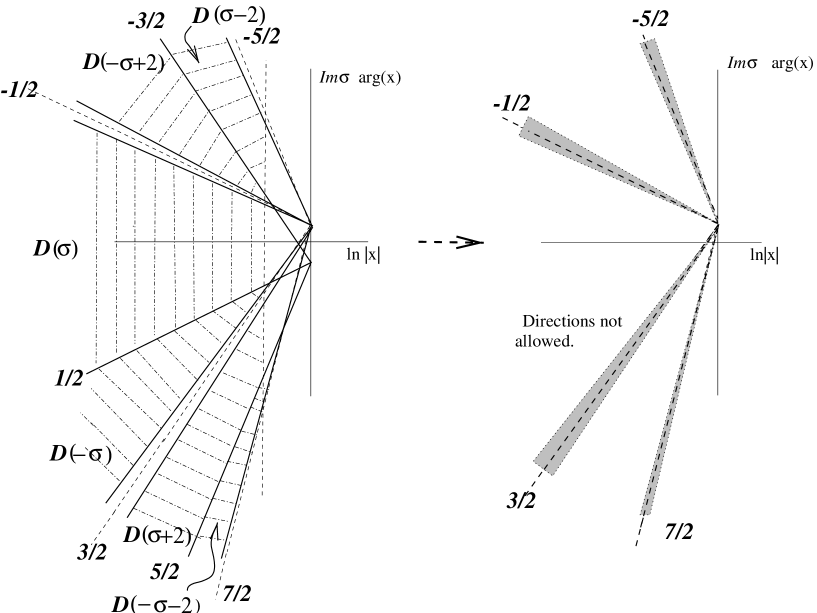
Figure 5: Domains for $\sigma={1\over 2}+i\Im\sigma$. The numbers close to the lines are their slopes. The small sectors around the dotted lines represented in the right figure are not contained in the union of the domains. If $x\to 0$ along a direction which ends in one of these sectors, we do not know the behavior of the transcendent.

If we draw, for the same $\theta_{2}$, the domains $B(\sigma)$, $B(-\sigma)$, $B(-\sigma+2)$, etc, defined in (30) we obtain strips in the $(\ln|x|,\Im\sigma\arg(x))$-plane which are certainly forbidden to Theorem 1 (see figure 6). In the strips we know nothing about the transcendent. We guess that there might be poles there, as we verify in one example later.

Figure 6:

What is the behavior along the directions not allowed by Theorem 1? In the very particular case $(x_{0},x_{1},x_{\infty})\in\{(2,2,2),(2,-2,-2),(-2,-2,2),(-2,2,-2)\}$ it is known that $PVI_{\mu=-1/2}$ has a 1-parameter family of classical solutions. The critical behavior of a branch for radial convergence to the critical points 0, 1 ,$\infty$ was computed in [28]:

$$y(x)=\left\{\matrix{-\ln(x)^{-2}(1+O(\ln(x)^{-1})),~{}~{}~{}~{}~{}x\to 0\cr\cr 1+\ln(1-x)^{-2}(1+O(\ln(1-x)^{-1})),~{}~{}~{}~{}~{}x\to 1\cr\cr-x\ln(1/x)^{-2}(1+O(\ln(1/x)^{-1}),~{}~{}~{}~{}~{}x\to\infty\cr}\right.$$

The branch is specified by $|\arg(x)|<\pi$, $|\arg(1-x)|<\pi$. This behavior is completely different from $\sim a(x)x^{1-\sigma}$ as $x\to 0$. Intuitively, as $x_{0}$ approaches the value 2, $1-\sigma$ approaches 0 and the decay of $y(x)\sim ax^{1-\sigma}$ becomes logarithmic. These solutions were called Chazy solutions in [28], because they can be computed as functions of solutions of the Chazy equation.

This section is devoted to the investigation of the critical behavior at $x=0$ in the regions not allowed in theorem 1.

5.1 Elliptic Representation

The transcendents of $PVI_{\mu}$ can be represented in the elliptic form [14]

$$y(x)=\wp\left({u(x)\over 2};\omega_{1}(x),\omega_{2}(x)\right)+{1+x\over 3}$$

where $\wp(z;\omega_{1},\omega_{2})$ is the Weierstrass elliptic function of half-periods $\omega_{1}$, $\omega_{2}$. $u(x)$ solves the non-linear differential equation

$${\cal L}(u)={\alpha\over x(1-x)}{\partial\over\partial u}\left[\wp\left({u\over 2};\omega_{1}(x),\omega_{2}(x)\right)\right],~{}~{}~{}\alpha={(2\mu-1)^{2}\over 2}$$ (33)

where the differential linear operator ${\cal L}$ applied to $u$ is

$${\cal L}(u):=x(1-x)~{}{d^{2}u\over dx^{2}}+(1-2x)~{}{du\over dx}-{1\over 4}~{}u.$$

The half-periods are two independent solutions of the hyper-geometric equation ${\cal L}(u)=0$:

$$\omega_{1}(x):={\pi\over 2}~{}F\left(x\right),~{}~{}~{}~{}\omega_{2}(x):=-{i\over 2}[F(x)\ln x+F_{1}(x)]$$

where $F(x)$ is the hyper-geometric function

$$F(x):=F\left({1\over 2},{1\over 2},1;x\right)=\sum_{n=0}^{\infty}{\left[\left({1\over 2}\right)_{n}\right]^{2}\over(n!)^{2}}x^{n},$$

and

$$F_{1}(x):=\sum_{n=0}^{\infty}{\left[\left({1\over 2}\right)_{n}\right]^{2}\over(n!)^{2}}2\left[\psi(n+{1\over 2})-\psi(n+1)\right]x^{n}$$

$$\psi(z)={d\over dz}\ln\Gamma(z),~{}~{}~{}\psi\left({1\over 2}\right)=-\gamma-2\ln 2,~{}~{}~{}\psi(1)=-\gamma,~{}~{}~{}\psi(a+n)=\psi(a)+\sum_{l=0}^{n-1}{1\over a+l}.$$

The solutions $u$ of (33) were not studied in the literature, so we did that and we proved a general result in Theorem 3. But first, we give a special example, already known to Picard.

Example: The equation $PVI_{\mu=1/2}$ has a two parameter family of solutions discovered by Picard [32] [30] [28]. It is easily obtained from (33). Since $\alpha=0$, $u$ solves the hyper-geometric equation ${\cal L}(u)=0$ and has the general form

$${u(x)\over 2}:=\nu_{1}\omega_{1}(x)+\nu_{2}\omega_{2}(x),~{}~{}~{}\nu_{i}\in{\bf C},~{}~{}~{}0\leq\Re\nu_{i}<2,~{}~{}~{}(\nu_{1},\nu_{2})\neq(0,0),$$

A branch of $y(x)$ is specified by a branch of $\ln x$ in $\omega_{2}(x)$. The monodromy data computed in [28] are

$$x_{0}=-2\cos\pi r_{1},~{}~{}~{}x_{1}=-2\cos\pi r_{2},~{}~{}~{}x_{\infty}=-2\cos\pi r_{3},$$

$$r_{1}={\nu_{2}\over 2},~{}~{}~{}r_{2}=1-{\nu_{1}\over 2},~{}~{}~{}r_{3}={\nu_{1}-\nu_{2}\over 2},~{}~{}~{}~{}\hbox{ for }\Re\nu_{1}>\Re\nu_{2}$$

$$r_{1}=1-{\nu_{2}\over 2},~{}~{}~{}r_{2}={\nu_{1}\over 2},~{}~{}~{}r_{3}={\nu_{2}-\nu_{1}\over 2},~{}~{}~{}~{}\hbox{ for }\Re\nu_{1}<\Re\nu_{2}.$$

The modular parameter is now a function of $x$:

$$\tau(x)={\omega_{2}(x)\over\omega_{1}(x)}={1\over\pi}(\arg x-i\ln|x|)+{4i\over\pi}\ln 2+O(x),~{}~{}~{}x\to 0.$$

We see that $\Im\tau>0$ as $x\to 0$. Now, if

$$\left|\Im{u(x)\over 4\omega_{1}}\right|<\Im\tau,$$ (34)

we can expand the Weierstrass function in Fourier series. Condition (34) becomes

$${1\over 2}\left|\Im\nu_{1}+{\Im\nu_{2}\over\pi}\arg(x)-{\Re\nu_{2}\over\pi}\ln|x|+{4\ln 2\over\pi}\Re\nu_{2}\right|<-{\ln|x|\over\pi}+{4\ln 2\over\pi}+O(x),~{}~{}~{}~{}\hbox{ as }x\to 0$$

For $\Im\nu_{2}\neq 0$ this can be written as follows:

$$(\Re\nu_{2}+2)\ln|x|+c_{1}<\Im\nu_{2}\arg(x)<(\Re\nu_{2}-2)\ln|x|+c_{2}.$$ (35)

$$c_{1}:=-\pi\Im\nu_{1}-4\ln 2~{}(\Re\nu_{2}+2),~{}~{}~{}~{}~{}c_{2}:=-\pi\Im\nu_{1}-4\ln 2~{}(\Re\nu_{2}-2)$$

On the other hands, if $\Im\nu_{2}=0$ any value of $\arg x$ is allowed. The Fourier expansion is

$$y(x)={x+1\over 3}+{1\over F(x)^{2}}\left[{1\over\sin^{2}\left(-{1\over 2}[i\nu_{2}(\ln(x)+{F_{1}(x)\over F(x)})-\pi\nu_{1}]\right)}-{1\over 3}+\right.$$

$$\left.+8\sum_{n=1}^{\infty}{x^{2n}\over e^{-2n{F_{1}(x)\over F(x)}}-x^{2n}}\sin^{2}\left(-{n\over 2}[i\nu_{2}(\ln(x)+{F_{1}(x)\over F(x)})-\pi\nu_{1}]\right)\right]$$

$$={x\over 2}+(1-{x\over 2}+O(x^{2}))\left[{1\over\sin^{2}\left(-{1\over 2}[i\nu_{2}(\ln(x)+{F_{1}(x)\over F(x)})-\pi\nu_{1}]\right)}+\right.$$

$$\left.-{1\over 4}\left[{e^{i\pi\nu_{1}}\over 16^{\nu_{2}-1}}\right]^{-1}x^{2-\nu_{2}}+O(x^{2}+x^{3-\nu_{2}}+x^{4-\nu_{2}})\right],~{}~{}~{}~{}~{}x\to 0\hbox{ in the domain }(\ref{dominio})$$

As far as radial convergence is concerned, we have:

a) $0<\Re\nu_{2}<2$,

$${1\over\sin^{2}(...)}=-{1\over 4}\left[{e^{i\pi\nu_{1}}\over 16^{\nu_{2}-1}}\right]~{}x^{\nu_{2}}~{}\bigl{(}1+O(|x^{\nu_{2}}|)\bigr{)},$$

and so

$$y(x)=\left\{-{1\over 4}\left[{e^{i\pi\nu_{1}}\over 16^{\nu_{2}-1}}\right]~{}x^{\nu_{2}}+{1\over 2}x-{1\over 4}\left[{e^{i\pi\nu_{1}}\over 16^{\nu_{2}-1}}\right]^{-1}x^{2-\nu_{2}}\right\}~{}\left(1+O(x^{\delta})\right),~{}~{}~{}~{}\delta>0.$$ (36)

This is the same critical behavior of Theorem 1. By virtue of the Proposition of section 4, the transcendent here coincides with $y(x;\sigma,a)$ of Theorem 1 if we identify $1-\sigma$ with $\nu_{2}$ for $0<\Re\nu_{2}<1$, or with $2-\nu_{2}$ for $1<\Re\nu_{2}<2$. In the case $\Re\nu_{2}=1$ the three terms $x^{\nu_{2}}$, $x$, $x^{2-\nu_{2}}$ have the same order and we find again the behavior (10) of Theorem 1 (oscillatory case):

$$y(x)=\left\{ax^{\nu_{2}}+{x\over 2}+{1\over 16a}x^{2-\nu_{2}}\right\}(1+O(x^{\delta}))=ax^{\nu_{2}}\left\{1+{1\over 2a}x^{-i\Im\nu_{2}}+{1\over 16a^{2}}x^{-2i\Im\nu_{2}}\right\}(1+O(x^{\delta})),$$

where $a=-{1\over 4}\left[{e^{i\pi\nu_{1}}\over 16^{\nu_{2}-1}}\right]$.

b) $\Re\nu_{2}=0$. Put $\nu_{2}=i\nu$ ( namely, $\sigma=1-i\nu$ ). The domain (35) is now (for sufficiently small $|x|$):

$$2\ln|x|-\pi\Im\nu_{1}-8\ln 2<\Im\nu_{2}\arg(x)<-2\ln|x|-\pi\Im\nu_{1}+8\ln 2,$$

or

$$2\ln|x|+\pi\Im\nu_{1}-8\ln 2<\Im\sigma\arg(x)<-2\ln|x|+\pi\Im\nu_{1}+8\ln 2.$$ (37)

For radial convergence we have

$$y(x)={1+O(x)\over\sin^{2}({\nu\over 2}\ln(x)+{\nu\over 2}{F_{1}(x)\over F(x)}+{\pi\nu_{1}\over 2})}+O(x).$$

This is an oscillating functions, and it may have poles. Suppose for example that $\nu_{1}$ is real. Since $F_{1}(x)/F(x)$ is a convergent power series ($|x|<1$) with real coefficients and defines a bounded function, then $y(x)$ has a sequence of poles on the positive real axis, converging to $x=0$.

In the domain (37) spiral convergence of $x$ to zero is also allowed and the critical behavior is (36) because $\arg x$ is not constant.

Finally, if $\nu=0$, namely $\nu_{2}=0$ (and then $x_{0}=2$) we have

$$y(x)={1\over\sin^{2}(\pi\nu_{1})}(1+O(|x|)).$$

The case b) in the above example is good to understand the limitation of Theorem 1 in giving a complete description of the behavior of Painlevé transcendents. Actually, Theorem 1 yields the behavior (36) in the domain $D(\sigma)\cup D(-\sigma)$ ($\Re\sigma=1$):

$$(1+\tilde{\sigma})\ln|x|+\theta_{1}\Im\sigma\leq\Im\sigma\arg x\leq(1-\tilde{\sigma})\ln|x|+\theta_{1}\Im\sigma,$$

where radial convergence to $x=0$ is not allowed. On the other hand, the transformations $\sigma\to\pm(\sigma-2)$, gives a further domain $D(\sigma-2)\cup D(-\sigma+2)$:

$$(-1+\tilde{\sigma})\ln|x|+\theta_{1}\Im\sigma\leq\Im\sigma\arg x\leq-(1+\tilde{\sigma})\ln|x|+\theta_{1}\Im\sigma,$$

but again it is not possible for $x$ to converge to $x=0$ along a radial path. Figure 7 shows $D(\sigma)\cup D(-\sigma)\cup D(2-\sigma)\cup D(\sigma-2)$. Note that a radial path would be allowed if it were possible to make $\tilde{\sigma}\to 1$. The interior of the set obtained as the limit for $\tilde{\sigma}\to 1$ of $D(\sigma)\cup D(-\sigma)\cup D(2-\sigma)\cup D(\sigma-2)$ is like (37). Actually, the intersection of (37) and $D(\sigma)\cup D(-\sigma)\cup D(2-\sigma)\cup D(\sigma-2)$ is never empty. On (37) the elliptic representation predicts an oscillating behavior and poles. So it is definitely clear that the “limit” of theorem 1 for $\tilde{\sigma}\to 1$ is not trivial.

Figure 7:

Remark on the example: For $\mu$ half integer all the possible values of $(x_{0},x_{1},x_{\infty})$ such that $x_{0}^{2}+x_{1}^{2}+x_{\infty}^{2}-x_{0}x_{1}x_{\infty}=4$ are covered by Chazy and Picard’s solutions, with the warning that for $\mu={1\over 2}$ the image (through birational transformations) of Chazy solutions is $y=\infty$. See [28].

We turn to the general case. The elliptic representation has been studied from the point of view of algebraic geometry in [27], but to our knowledge Theorem 3 and its Corollary, both stated in the Introduction, are the first general result about its critical behavior appearing in the literature.

We prove Theorem 3 in section 10. Here we prove the Corollary. The critical behavior is obtained expanding $y(x)$ in Fourier series:

$$\wp\left({u\over 2};\omega_{1},\omega_{2}\right)=-{\pi^{2}\over 12\omega_{1}^{2}}+{2\pi^{2}\over\omega_{1}^{2}}\sum_{n=1}^{\infty}{ne^{2\pi in\tau}\over 1-e^{2\pi in\tau}}\left(1-\cos\left(n{\pi u\over 2\omega_{1}}\right)\right)+{\pi^{2}\over 4\omega_{1}^{2}}~{}{1\over\sin^{2}\left({\pi u\over 4\omega_{1}}\right)}$$ (38)

The expansion can be performed if $\Im\tau(x)>0$ and $\left|\Im\left({u(x)\over\omega_{1}(x)}\right)\right|<\Im\tau$; these conditions are satisfied in ${\cal D}(r;\nu_{1},\nu_{2})$. Let’s put $F_{1}/F=-4\ln 2+g(x)$, where $g(x)=O(x)$. Taking into account (38) and Theorem 3, the expansion of $y(x)$ for $x\to 0$ in ${\cal D}(r;\nu_{1},\nu_{2})$ is

$$y(x)=\left[{1+x\over 3}-{\pi^{2}\over 12\omega_{1}(x)^{2}}\right]+{\pi^{2}\over\omega_{1}(x)^{2}}\sum_{n=1}^{\infty}{n\over 1-\left({e^{g(x)}\over 16}\right)^{2n}x^{2n}}\left\{2\left({e^{g(x)}\over 16}\right)^{2n}x^{2n}+\right.$$

$$\left.-e^{n(\nu_{2}+2)g(x)}\left[{e^{i\pi\nu_{1}}\over 16^{2+\nu_{2}}}x^{2+\nu_{2}}\right]^{n}e^{in\pi{v(x)\over\omega_{1}(x)}}-e^{n(2-\nu_{2})g(x)}\left[{e^{-i\pi\nu_{1}}\over 16^{2-\nu_{2}}}x^{2-\nu_{2}}\right]^{n}e^{-i\pi n{v(x)\over\omega_{1}(x)}}\right\}+$$

$$+{\pi^{2}\over 4\omega_{1}(x)^{2}}{1\over\sin^{2}\left(-i{\nu_{2}\over 2}\ln x+i{\nu_{2}\over 2}\ln 16+{\pi\nu_{1}\over 2}-i{\nu_{2}\over 2}g(x)+{\pi v(x)\over 2\omega_{1}(x)}\right)}$$

We observe that $\omega_{1}(x)\equiv{\pi\over 2}F(x)={\pi\over 2}(1+{1\over 4}x+O(x^{2}))$, ${1+x\over 3}-{\pi^{2}\over 12\omega_{1}(x)^{2}}\equiv{1+x\over 3}-{1\over 3F(x)}={1\over 2}x\bigl{(}1+O(x)\bigr{)}$, $e^{g(x)}=1+O(x)$ and

$$e^{\pm i\pi{v(x)\over\omega_{1}(x)}}=1+O\left(|x|+\left|{e^{-i\pi\nu_{1}}\over 16^{2-\nu_{2}}}x^{2-\nu_{2}}\right|+\left|{e^{i\pi\nu_{1}}\over 16^{\nu_{2}}}x^{\nu_{2}}\right|\right)$$

In order to single out the leading terms, we observe that we are dealing with the powers $x$, $x^{2-\nu_{2}}$, $x^{\nu_{2}}$ in ${\cal D}(r;\nu_{1},\nu_{2})$. If $0<\nu_{2}<2$ (the only allowed real values of $\nu_{2}$) $|x^{\nu_{2}}|$ is leading if $0<\nu_{2}<1$ and $|x^{2-\nu_{2}}|$ is leading if $1<\nu_{2}<2$. We have

$${1\over\sin^{2}(...)}=-4{e^{i\pi\nu_{1}}\over 16^{\nu_{2}}}x^{\nu_{2}}\left[1+O(|x|+|x^{\nu_{2}}|+|x^{2-\nu_{2}}|)\right]$$

Thus, there exists $0<\delta<1$ (explicitly computable in terms of $\nu_{2}$) such that

$$y(x)=\left[{1\over 2}x-{1\over 4}\left[{e^{i\pi\nu_{1}}\over 16^{\nu_{2}-1}}\right]x^{\nu_{2}}-{1\over 4}\left[{e^{i\pi\nu_{1}}\over 16^{\nu_{2}-1}}\right]^{-1}x^{2-\nu_{2}}\right](1+O(x^{\delta}))$$

$$=\left\{\matrix{\sin^{2}\left({\pi\nu_{1}\over 2}\right)~{}x~{}(1+O(x^{\delta})),~{}~{}~{}\hbox{ if }\nu_{2}=1\cr\cr-{1\over 4}\left[{e^{i\pi\nu_{1}}\over 16^{\nu_{2}-1}}\right]x^{\nu_{2}}(1+O(x^{\delta}))~{}~{}~{}\hbox{ if }0<\nu_{2}<1\cr\cr-{1\over 4}\left[{e^{i\pi\nu_{1}}\over 16^{\nu_{2}-1}}\right]^{-1}x^{2-\nu_{2}}(1+O(x^{\delta}))~{}~{}~{}\hbox{ if }1<\nu_{2}<2\cr}\right.$$

This behavior coincides with that of Theorem 1 for $\sigma=0$ in the first case, $\sigma=1-\nu_{2}$ in the second, $\sigma=\nu_{2}-1$ in the third.

We turn to the case $\Im\nu_{2}\neq 0$. We consider a path contained in ${\cal D}(r;\nu_{1},\nu_{2})$ of equation

$$\Im\nu_{2}\arg(x)=(\Re\nu_{2}-{\cal V})\ln|x|+b,~{}~{}~{}~{}0\leq{\cal V}\leq 2$$ (39)

with a suitable constant $b$ (the path connects some $x_{0}\in{\cal D}(r;\nu_{1},\nu_{2})$ to $x=0$, therefore $b=\Im\nu_{2}\arg x_{0}-(\Re\nu_{2}-{\cal V})\ln|x_{0}|$). We have$|x^{2-\nu_{2}}|=|x|^{2-{\cal V}}e^{b}$, $|x^{\nu_{2}}|=|x|^{\cal V}e^{-b}$ and so

$$|x^{\nu_{2}}|~{}~{}\hbox{ is leading for }~{}0\leq{\cal V}<1,$$

$$|x^{\nu_{2}}|,~{}|x|,~{}|x^{2-\nu_{2}}|~{}~{}\hbox{ have the same order for }~{}{\cal V}=1,$$

$$|x^{2-\nu_{2}}|~{}~{}\hbox{ is leading for }~{}1<{\cal V}\leq 2.$$

If ${\cal V}=0$,

$$\left|{e^{i\pi\nu_{1}}\over 16^{\nu_{2}}}x^{\nu_{2}}\right|<r,~{}~{}~{}~{}~{}~{}\hbox{ but }~{}x^{\nu_{2}}\not\to 0~{}\hbox{ as }~{}x\to 0.$$

If ${\cal V}=2$,

$$\left|{e^{-i\pi\nu_{1}}\over 16^{2-\nu_{2}}}x^{2-\nu_{2}}\right|<r~{}~{}~{}~{}~{}~{}\hbox{ but }~{}x^{2-\nu_{2}}\not\to 0~{}\hbox{ as }~{}x\to 0.$$

This also implies that $v(x)\not\to 0$ as $x\to 0$ along the paths with ${\cal V}=0$ or ${\cal V}=2$, while $v(x)\to 0$ for all other values $0<{\cal V}<2$. We conclude that:

a) If $x\to 0$ in ${\cal D}(r;\nu_{1},\nu_{2})$ along (39) for ${\cal V}\neq 0,2$, then

$$y(x)=\left[{1\over 2}x-{1\over 4}\left[{e^{i\pi\nu_{1}}\over 16^{\nu_{2}-1}}\right]x^{\nu_{2}}-{1\over 4}\left[{e^{i\pi\nu_{1}}\over 16^{\nu_{2}-1}}\right]^{-1}x^{2-\nu_{2}}\right](1+O(x^{\delta})),~{}~{}~{}~{}0<\delta<1.$$

The three leading terms have the same order if the convergence is along a path asymptotic to (39) with ${\cal V}=1$. Namely

$$y(x)=x~{}\sin^{2}\left(i{1-\nu_{2}\over 2}\ln x+{\pi\nu_{1}\over 2}+2i(\nu_{2}-1)\ln 2\right)~{}\bigl{(}1+O(x)\bigr{)}~{}~{}\hbox{ for }{\cal V}=1.$$

Otherwise

$$y(x)=-{1\over 4}\left[{e^{i\pi\nu_{1}}\over 16^{\nu_{2}-1}}\right]x^{\nu_{2}}(1+O(x^{\delta}))~{}~{}\hbox{ for }0<{\cal V}<1,$$

or

$$y(x)=-{1\over 4}\left[{e^{i\pi\nu_{1}}\over 16^{\nu_{2}-1}}\right]^{-1}x^{2-\nu_{2}}(1+O(x^{\delta}))~{}~{}\hbox{ for }1<{\cal V}<2.$$

This is the behavior of Theorem 1 with $1-\sigma=\nu_{2}$ or $2-\nu_{2}$.

Important Observation: Let $\nu_{2}=1-\sigma$ and consider the intersection ${\cal D}(r;\nu_{1},\nu_{2})\cap\cal D(\sigma)$ in the $(\ln|x|,\Im\nu_{2}\arg(x))$-plane. It is never empty. See figure 7. We choose $\nu_{1}$ such that $a=-{1\over 4}\left[{e^{i\pi\nu_{1}}\over 16^{\nu_{2}-1}}\right]$. According to the Proposition in section 4, the transcendent of the elliptic representation and $y(x;\sigma,a)$ of Theorem 1 coincide on the intersection. Equivalently, we can choose the identification $1-\sigma=2-\nu_{2}$ and repeat the argument.

b) If ${\cal V}=0$ the term

$${1\over\sin^{2}\left(-i{\nu_{2}\over 2}\ln x+\left[i{\nu_{2}\over 2}\ln 16+{\pi\nu_{1}\over 2}\right]-i{\nu_{2}\over 2}g(x)+{\pi v(x)\over 2\omega_{1}(x)}\right)}$$

is oscillatory as $x\to 0$ and does not vanish. Note that there are no poles because the denominator does not vanish in ${\cal D}(r;\nu_{1},\nu_{2})$ since $\left|{e^{i\pi\nu_{1}}\over 16^{\nu_{2}}}x^{\nu_{2}}\right|<r<1$. Then

$$y(x)=O(x)+{1\over F(x)^{2}}{1\over\sin^{2}\left(-i{\nu_{2}\over 2}\ln x+\left[i{\nu_{2}\over 2}\ln 16+{\pi\nu_{1}\over 2}\right]-i{\nu_{2}\over 2}g(x)+{v(x)\over F(x)}\right)}$$

$$={1+O(x)\over\sin^{2}\left(-i{\nu_{2}\over 2}\ln x+\left[i{\nu_{2}\over 2}\ln 16+{\pi\nu_{1}\over 2}\right]+\sum_{m=1}^{\infty}c_{0m}(\nu_{2})\left[{e^{i\pi\nu_{1}}\over 16^{\nu_{2}}}x^{\nu_{2}}\right]^{m}\right)}+O(x)$$

The last step is obtained taking into account the non vanishing term in (13) and ${\pi v(x)\over 2\omega_{1}(x)}={v(x)\over F(x)}=v(x)(1+O(x))$.

c) If ${\cal V}=2$ the series

$$-\sum_{n=1}^{\infty}{n\over 1-\left({e^{g(x)}\over 16}\right)^{2n}x^{2n}}~{}e^{n(2-\nu_{2})g(x)}\left[{e^{-i\pi\nu_{1}}\over 16^{2-\nu_{2}}}x^{2-\nu_{2}}\right]^{n}e^{-i\pi n{v(x)\over\omega_{1}(x)}}$$

which appears in $y(x)$ is oscillating. Simplifying we obtain:

$$y(x)=O(x)-4(1+O(x))~{}\sum_{n=1}^{\infty}n\left[{e^{-i\pi\nu_{1}}\over 16^{2-\nu_{2}}}x^{2-\nu_{2}}\right]^{n}~{}e^{-i\pi n{v(x)\over\omega_{1}(x)}}$$

$$={1+O(x)\over\sin^{2}\left(i{2-\nu_{2}\over 2}\ln x+\left[i{\nu_{2}-2\over 2}\ln 16+{\pi\nu_{1}\over 2}\right]+\sum_{m=1}^{\infty}b_{0m}(\nu_{2})\left[{e^{-i\pi\nu_{1}}\over 16^{2-\nu_{2}}}x^{\nu_{2}}\right]^{m}\right)}+O(x)$$

The observation at the end of point a) makes it possible to investigate the behavior of the transcendents of Theorem 1 along a path (8) with $\Sigma=1$. The path (8) coincides with (39) for ${\cal V}=0$ if we define $1-\sigma:=\nu_{2}$, for ${\cal V}=2$ if we define $1-\sigma=2-\nu_{2}$.

In particular, we can analyze the radial convergence when $\Re\sigma=1$. We identify $\nu_{2}=1-\sigma$ and choose $\nu_{2}=i\nu$, $\nu\neq 0$ real. Namely, $\sigma=1-i\nu$. Let $x\to 0$ in ${\cal D}(r;\nu_{1},i\nu)$ along the line $\arg(x)$= constant (it is the line with ${\cal V}=0$). We have

$$y(x)={1\over F(x)^{2}}{1\over\sin^{2}\left({\nu\over 2}\ln x-\nu\ln 16+{\pi\over 2}\nu_{1}+{\nu\over 2}g(x)+{\pi v(x)\over 2\omega_{1}(x)}\right)}+O(x)$$

$$={1+O(x)\over\sin^{2}\left({\nu\over 2}\ln x-\nu\ln 16+{\pi\nu_{1}\over 2}+\sum_{m=1}^{\infty}c_{0m}(\nu)\left[\left({e^{i\pi\nu_{1}}\over 16^{i\nu}}\right)x^{i\nu}\right]^{m}+O(x)\right)}+O(x)$$

$$={1+O(x)\over\sin^{2}\left({\nu\over 2}\ln x-\nu\ln 16+{\pi\nu_{1}\over 2}+\sum_{m=1}^{\infty}c_{0m}(\nu)\left[\left({e^{i\pi\nu_{1}}\over 16^{i\nu}}\right)x^{i\nu}\right]^{m}\right)}$$

The last step is possible because $\sin(f(x)+O(x))=\sin(f(x))+O(x)=\sin(f(x))\bigl{(}1+O(x)\bigr{)}$ if $f(x)\not\to 0$ as $x\to 0$; this is our case for $f(x)={\nu\over 2}\ln x-\nu\ln 16+{\pi\nu_{1}\over 2}+\sum_{m=1}^{\infty}c_{om}(\nu)\left[\left({e^{i\pi\nu_{1}}\over 16^{i\nu}}\right)x^{i\nu}\right]^{m}$ in ${\cal D}$.

We observe that for $\Re\sigma=1$ we have a limitation on $\arg(x)$ in ${\cal D}(r;\nu_{1},i\nu)$, namely

$$-\pi\Im\nu_{1}-\ln r<\nu\arg(x)$$ (40)

This is the analogous of the limitation imposed by $B(\sigma,a;\theta_{2},\tilde{\sigma})$ of (30).

Remark: If $\Im\nu_{2}\neq 0$, the freedom $\nu_{2}\mapsto\nu_{2}+2N$, $N\in{\bf Z}$, is the analogous of the freedom $\sigma\mapsto\pm\sigma+2n$. Moreover, Theorem 3 yields different critical behaviors for the same transcendent on the different domains corresponding to $\nu_{2}+2N$.

As a last remark we observe that the coefficients in the expansion of $v(x)$ can be computed by direct substitution of $v$ into the elliptic form of $PVI_{\mu}$, the right hand-side being expanded in Fourier series.

5.2 Shimomura’s Representation

In [37] and [19] S. Shimomura proved the following statement for the Painlevé VI equation with any value of the parameters $\alpha,\beta,\gamma,\delta$. For any complex number $k$ and for any $\sigma\not\in(-\infty,0]\cup[1,+\infty)$ there is a sufficiently small $r$ such that the Painlevé VI equation for given $\alpha,\beta,\gamma,\delta$ has a holomorphic solution in the domain

$${\cal D}_{s}(r;\sigma,k)=\{{x}\in\tilde{C_{0}}~{}|~{}|x|<r,~{}|e^{-k}{x}^{1-\sigma}|<r,~{}|e^{k}{x}^{\sigma}|<r\}$$

with the following representation:

$$y({x};\sigma,k)={1\over\cosh^{2}({\sigma-1\over 2}\ln{x}+{k\over 2}+{v({x})\over 2})},$$

where

$$v({x})=\sum_{n\geq 1}a_{n}(\sigma){x}^{n}+\sum_{n\geq 0,~{}m\geq 1}b_{nm}(\sigma){x}^{n}(e^{-k}{x}^{1-\sigma})^{m}+\sum_{n\geq 0,~{}m\geq 1}c_{nm}(\sigma){x}^{n}(e^{k}{x}^{\sigma})^{m},$$

$a_{n}(\sigma),b_{nm}(\sigma),c_{nm}(\sigma)$ are rational functions of $\sigma$ and the series defining $v({x})$ is convergent (and holomorphic) in ${\cal D}(r;\sigma,k)$. Moreover, there exists a constant $M=M(\sigma)$ such that

$$|v(x)|\leq M(\sigma)~{}\left(|x|+|e^{-k}{x}^{1-\sigma}|+|e^{k}{x}^{\sigma}|\right).$$ (41)

The domain ${\cal D}(r;\sigma,k)$ is specified by the conditions:

$$|x|<r,~{}~{}~{}\Re\sigma\ln|x|+[\Re k-\ln r]<\Im\sigma\arg(x)<(\Re\sigma-1)\ln|x|+[\Re k+\ln r].$$ (42)

This is an open domain in the plane $(\ln|x|,\arg(x))$. It can be compared with the domain $D(\epsilon;\sigma,\theta_{1},\theta_{2})$ of Theorem 1 (figure 8). Note that (42) imposes a limitation on $\arg(x)$. For example, if $\Re\sigma=1$ we have

$$\Im\sigma\arg(x)<[\Re k+\ln r],~{}~{}~{}~{}~{}(\ln r<0)$$

This is similar to (40). We will show that Shimomura’s transcendents coincide with those of Theorem 1 (see point a.1) below). So, the above limitation turns out to be the analogous of the limitation imposed to $D(\epsilon;\sigma;\theta_{1},\theta_{2})$ by $B(\sigma,a;\theta_{2},\tilde{\sigma})$ of (30).

Like the elliptic representation, Shimomura’s allows us to investigate what happens when ${x}\to 0$ along a path (8) with $\Sigma=1$, contained in ${\cal D}_{s}(r;\sigma,k)$. It is a radial path if $\Re\sigma=1$. Along (8) we have $|x^{\sigma}|=|x|^{\Sigma}e^{-b}$. We suppose $\Im\sigma\neq 0$.

a) $0\leq\Sigma<1$. We observe that $|x^{1-\sigma}e^{-k}|\to 0$ as $x\to 0$ along the line. Then:

$$y({x};\sigma,k)={1\over\cosh^{2}({\sigma-1\over 2}\ln x+{k\over 2}+{v({x})\over 2})}={4\over x^{\sigma-1}e^{k}e^{v(x)}+x^{1-\sigma}e^{-k}e^{-v(x)}+2}$$

$$=4e^{-k}e^{-v(x)}x^{1-\sigma}~{}{1\over(1+e^{-k}e^{-v(x)}x^{1-\sigma})^{2}}=4e^{-k}e^{-v(x)}x^{1-\sigma}~{}\left(1+e^{-v(x)}O(|e^{-k}x^{1-\sigma}|)\right).$$

Two sub-cases:

a.1) $\Sigma\neq 0$. Then $|x^{\sigma}e^{k}|\to 0$ and $v(x)\to 0$ (see (41)). Thus

$$y({x};\sigma,k)=4e^{-k}x^{1-\sigma}\left(1+O(|x|+|e^{k}x^{\sigma}|+|e^{-k}x^{1-\sigma}|)\right)$$

By the Proposition in section 4, $y(x;\sigma,k)$ and $y(x;\sigma,a)$ coincide, for $a=4e^{-k}$, in $D_{s}(r;\sigma,k)\cap D(\epsilon;\sigma;\theta_{1},\theta_{2})$. The intersection is not empty for any $\theta_{1}$, $\theta_{2}$. See figure 8.

Figure 8: The domains ${\cal D}_{s}(r;\sigma,k)$ and $D(\epsilon;\sigma;\theta_{1},\theta_{2},\tilde{\sigma})$

a.2) $\Sigma=0$. $|x^{\sigma}e^{k}|\to$ constant$<r$, so $|v(x)|$ does not vanish. Then

$$y(x)=a(x)x^{1-\sigma}~{}\left(1+O(|e^{-k}x^{1-\sigma}|)\right),~{}~{}~{}~{}a(x)=4e^{-k}e^{-v(x)},$$

and $a(x)$ must coincide with (10) of Theorem 1:

b) $\Sigma=1$. In this case Theorem 1 fails. Now $|x^{1-\sigma}e^{-k}|\to$ (constant$\neq 0)<r$. Therefore $y(x)$ does not vanish as $x\to 0$. We keep the representation

$$y({x};\sigma,k)={1\over\cosh^{2}({\sigma-1\over 2}\ln x+{k\over 2}+{v({x})\over 2})}\equiv{1\over\sin^{2}(i{\sigma-1\over 2}\ln x+i{k\over 2}+i{v({x})\over 2}-{\pi\over 2})}$$

$v(x)$ does not vanish and $y({x})$ is oscillating as ${x}\to 0$, with no limit. We remark that like in the elliptic representation, $\cosh^{2}(...)$ does not vanish in ${\cal D}_{s}(r;\sigma,k)$, so we do not have poles. Figure 9 synthesizes points a.1), a.2), b).

Figure 9: Critical behavior of $y(x;\sigma,k)$ along different lines in ${\cal D}_{s}(r;\sigma,k)$

As an application, we consider the case $\Re\sigma=1$, namely $\sigma=1-i\nu,$ $\nu\in\bf{R}\backslash\{0\}$. Then, the path corresponding to $\Sigma=1$ is a radial path in the $x$-plane and

$$y({x};1-i\nu,k)={1+O(x)\over\sin^{2}\left({\nu\over 2}\ln(x)+{ik\over 2}-{\pi\over 2}+{i\over 2}\sum_{~{}m\geq 1}b_{0m}(\sigma)(e^{-k}x^{1-\sigma})^{m}\right)}$$

6 Analytic Continuation of a Branch

Figure 10: Base point and loops in ${\bf C}\backslash\{0,1\}$ and in ${\bf CP}^{1}\backslash\{0,1,\infty\}$.

We describe the analytic continuation of the transcendent $y(x;\sigma,a)$. We choose a basis $\gamma_{0}$, $\gamma_{1}$ of two loops around 0 and 1 respectively in the fundamental group $\pi({\bf P}^{1}\backslash\{0,1,\infty\},b)$, where $b$ is the base-point (figure 10). The analytic continuation of a branch $y(x;x_{0},x_{1},x_{\infty})$ along paths encircling $x=0$ and $x=1$ (a loop around $x=\infty$ is homotopic to the product of $\gamma_{0}$, $\gamma_{1}$) is given by the action of the group of the pure braids on the monodromy data. This action is computed in [13], to which we refer. For a counter-clockwise loop around 0 we have to transform ($x_{0},x_{1},x_{\infty}$) by the action of the braid $\beta_{1}^{2}$, where

$$\beta_{1}:~{}~{}(x_{0},x_{1},x_{\infty})\mapsto(-x_{0},x_{\infty}-x_{0}x_{1},x_{1})$$

$$\beta_{1}^{2}:~{}~{}~{}~{}(x_{0},x_{1},x_{\infty})\mapsto(x_{0},~{}x_{1}+x_{0}x_{\infty}-x_{1}x_{0}^{2},~{}x_{\infty}-x_{0}x_{1})$$

The analytic continuation of the branch $y(x;x_{0},x_{1},x_{\infty})$ is the new branch $y(x;x_{0},~{}x_{1}+x_{0}x_{\infty}-x_{1}x_{0}^{2},~{}x_{\infty}-x_{0}x_{1})$. For a counter-clockwise loop around 1 we need the braid $\beta_{2}^{2}$, given by

$$\beta_{2}:~{}~{}(x_{0},x_{1},x_{\infty})\mapsto(x_{\infty},-x_{1},x_{0}-x_{1}x_{\infty})$$

$$\beta_{2}^{2}:~{}~{}(x_{0},x_{1},x_{\infty})\mapsto(x_{0}-x_{1}x_{\infty},~{}x_{1},~{}x_{\infty}+x_{0}x_{1}-x_{\infty}x_{1}^{2})$$

The analytic continuation of $y(x;x_{0},x_{1},x_{\infty})$ is the new branch $y(x;x_{0}-x_{1}x_{\infty},~{}x_{1},~{}x_{\infty}+x_{0}x_{1}-x_{\infty}x_{1}^{2})$. A generic loop ${\bf P}^{1}\backslash\{0,1,\infty\}$ is represented by a braid $\beta$, which is a product of factors $\beta_{1}$ and $\beta_{2}$. The braid $\beta$ acts on $(x_{0},x_{1},x_{\infty})$ and gives a new triple $(x_{0}^{\beta},x_{1}^{\beta},x_{\infty}^{\beta})$ and a new branch $y(x;x_{0}^{\beta},x_{1}^{\beta},x_{\infty}^{\beta})$.

On the other hand, $y(x;x_{0},x_{1},x_{\infty})$ is the branch of a transcendent which has analytic continuation on the universal covering of ${\bf P}^{1}\backslash\{0,1,\infty\}$. We still denote this transcendent by $y(x;x_{0},x_{1},x_{\infty})$, where $x$ is now regarded as a point in the universal covering. A loop transforms $x$ to a new point $x^{\prime}$ in the covering. The transcendent at $x^{\prime}$ is $y(x^{\prime};x_{0},x_{1},x_{\infty})$. Let $\beta$ be the corresponding braid. We have:

$$y(x;x_{0}^{\beta},x_{1}^{\beta},x_{\infty}^{\beta})=y(x^{\prime};x_{0},x_{1},x_{\infty})$$ (43)

Let $\sigma$, $a$ be associated to $(x_{0},x_{1},x_{\infty})$ according to Theorem 2. Let $x\in D(\sigma)$. At $x$ we have $y(x;x_{0},x_{1},x_{\infty})=y(x;\sigma,a)$. Let $\sigma^{\beta}$, $a^{\beta}=a(\sigma^{\beta};x_{0}^{\beta},x_{1}^{\beta},x_{\infty}^{\beta})$ be associated to $(x_{0}^{\beta},x_{1}^{\beta},x_{\infty}^{\beta})$. If $D(\sigma)\cap D(\sigma^{\beta})$ is not empty and $x$ also belongs to $D(\sigma^{\beta})$, then $y(x;x_{0}^{\beta},x_{1}^{\beta},x_{\infty}^{\beta})=y(x;\sigma^{\beta},a^{\beta})$ at $x$. If $x\not\in D(\sigma^{\beta})$, it belongs to one and only one of the domains $D(\pm\sigma^{\beta}+2n)$ and $y(x;x_{0}^{\beta},x_{1}^{\beta},x_{\infty}^{\beta})=y(x;\pm\sigma^{\beta}+2n,\tilde{a}^{\beta})$ at $x$, where $\tilde{a}^{\beta}=a(\pm\sigma^{\beta}+2n;x_{0}^{\beta},x_{1}^{\beta},x_{\infty}^{\beta})$. We note however that if $\Re\sigma^{\beta}=1$, it may happen that $x$ lies in the strip between $B(\sigma^{\beta})$ and $B(2-\sigma^{\beta})$, where there may be poles (see the beginning of section 5). In this case, we are not able to describe the analytic continuation (actually, the new branch may have a pole in $x$). But in this case, we can slightly change $\arg x$ in such a way that $x$ falls in a domain $D(\pm\sigma^{\beta}+2n)$.

As an example, let us start at $x\in D(\sigma)$; we perform the loop $\gamma_{1}$ around $1$ and we go back to $x$. If $x$ also belongs to $D(\sigma^{\beta_{2}^{2}})$ the transformation is

$$\gamma_{1}:~{}y(x;\sigma,a)\longrightarrow y(x;\sigma^{\beta_{2}^{2}},a^{\beta_{2}^{2}}).$$

If $x\not\in D(\sigma^{\beta_{2}^{2}})$ but $x$ belong to one of the $D(\pm\sigma^{\beta_{2}^{2}}+2n)$ we have

$$y(x;\sigma,a)\longrightarrow y(x;\pm\sigma^{\beta_{2}^{2}}+2n,\tilde{a}^{\beta_{2}^{2}}).$$

Again, let us start at $x\in D(\sigma)$; we perform the loop $\gamma_{0}$ around $0$ and we go back to $x$. The transformation of $(\sigma,a)$ according to the braid $\beta_{1}$ is

$$(\sigma^{\beta_{1}^{2}},a^{\beta_{1}^{2}})=(\sigma,ae^{-2\pi i\sigma})$$ (44)

as it follows from the fact that $x_{0}$ is not affected by $\beta_{1}^{2}$, then $\sigma$ does not change, and from the explicit computation of $a(\sigma,x_{0}^{\beta_{1}^{2}},x_{1}^{\beta_{1}^{2}},x_{\infty}^{\beta_{1}^{2}})$ through Theorem 2 (we will do it at the end of section 9). Therefore, the effect of $\gamma_{0}$ is

$$\gamma_{0}:~{}y(x;\sigma,a)\longrightarrow y(x;\sigma^{\beta_{1}^{2}},a^{\beta_{1}^{2}})=y(x;\sigma,ae^{-2\pi i\sigma})$$

Since we are considering a loop around $0$, it makes sense to consider is as a loop in ${\bf C}\backslash\{0\}\cap\{|x|<\epsilon\}$. The loop is $x\mapsto x^{\prime}=e^{2\pi i}x$. Suppose that also $x^{\prime}\in D(\sigma)$. Then, we can represent the analytic continuation on the universal covering as

$$y(x;\sigma,a)\longrightarrow y(x^{\prime};\sigma,a)$$

On the other hand, according to (43), we must have $y(x^{\prime};\sigma,a)=y(x;\sigma^{\beta_{1}^{2}},a^{\beta_{1}^{2}})$. This is immediately verified because:

$$y(x^{\prime};\sigma,a)=a[x^{\prime}]^{1-\sigma}\left(1+O\left(\left|x^{\prime}\right|^{\delta}\right)\right)$$

$$=ae^{-2\pi i\sigma}x^{1-\sigma}(1+O(|x|^{\delta}))\equiv y(x;\sigma,ae^{-2\pi i\sigma})$$

Thus Theorem 1 is in accordance with the analytic continuation obtained by the action of the braid group.

Figure 11: Analytic continuation of a branch for a loop around $x=0$ and a loop around $x=1$. We also draw the analytic continuation on the universal covering

7 Singular Points $x=1$, $x=\infty$ (Connection Problem)

In this section we restore the notation $\sigma^{(0)}$ and $a^{(0)}$ to denote the parameters of Theorem 1 near the critical point $x=0$. We describe now the analogous of Theorem 1 near $x=1$ and $x=\infty$. The three critical points $0$, $1$, $\infty$ are equivalent thanks to the symmetries discussed in [30] and [13].

a) Let

$$x={1\over t}~{}~{}~{}~{}y(x):={1\over t}~{}\hat{y}(t)$$ (45)

Then $y(x)$ is a solution of $PVI_{\mu}$ (variable $x$) if and only if $\hat{y}(t)$ is a solution of $PVI_{\mu}$ (variable $t$). The singularities $0$ and $\infty$ are exchanged. Theorem 1 holds for $\hat{y}(t)$ at $t=0$ with some parameters $\sigma$, $a$ that we call now $\sigma^{(\infty)}$, $a^{(\infty)}$. Then, we go back to $y(x)$ and find a transcendent $y(x;\sigma^{(\infty)},a^{(\infty)})$ with behavior

$$y({x};\sigma^{(\infty)},a^{(\infty)})=a^{(\infty)}{{x}}^{\sigma^{(\infty)}}\left(1+O({1\over|x|^{\delta}})\right)~{}~{}~{}~{}~{}{x}\to\infty$$ (46)

in

$$D(M;\sigma^{(\infty)};\theta_{1},\theta_{2},\tilde{\sigma}):=\{{x}\in\widetilde{{\bf C}\backslash\{\infty\}}\hbox{ s.t. }|x|>M,~{}e^{-\theta_{1}\Im\sigma^{(\infty)}}|x|^{-\tilde{\sigma}}\leq|{x}^{-\sigma^{(\infty)}}|\leq e^{-\theta_{2}\Im\sigma^{(\infty)}}$$

$$0<\tilde{\sigma}<1\}$$ (47)

where $M>0$ is sufficiently big and $0<\delta<1$ is small (figure 12).

Figure 12: Some examples of the domain $D(M;\sigma;\theta_{1},\theta_{2},\tilde{\sigma})$

b) Let

$$x=1-t,~{}~{}~{}~{}y(x)=1-\hat{y}(t)$$ (48)

$y(x)$ satisfies $PVI_{\mu}$ if and only if $\hat{y}(t)$ satisfies $PVI_{\mu}$. Theorem 1 holds for $\hat{y}(t)$ at $t=0$ with some parameters $\sigma$, $a$ that we now call $\sigma^{(1)}$ and $a^{(1)}$. Going back to $y(x)$ we obtain a transcendent $y(x;\sigma^{(1)},a^{(1)})$ such that

$$y({x},\sigma^{(1)},a^{(1)})=1-a^{(1)}(1-{x})^{1-\sigma^{(1)}}(1+O(|1-x|^{\delta}))~{}~{}~{}~{}{x}\to 1$$ (49)

in

$$D(\epsilon;\sigma^{(1)};\theta_{1},\theta_{2},\tilde{\sigma}):=\{{x}\in\widetilde{{\bf C}\backslash\{1\}}\hbox{ s.t. }|1-x|<\epsilon,~{}~{}e^{-\theta_{1}\Im\sigma}|1-x|^{\tilde{\sigma}}\leq|(1-{x})^{\sigma^{(1)}}|\leq e^{-\theta_{2}\Im\sigma},$$

$$0<\tilde{\sigma}<1\}$$ (50)

Consider a branch $y(x;x_{0},x_{1},x_{\infty})$. The symmetries in a) and b) affect the monodromy data, according to the following formulae proved in [13]:

$$y(x;x_{0},x_{1},x_{\infty})={1\over t}\hat{y}(t;x_{\infty},-x_{1},x_{0}-x_{1}x_{\infty}),~{}~{}~{}~{}x={1\over t}$$ (51)

$$y(x;x_{0},x_{1},x_{\infty})=1-\hat{y}(t;x_{1},x_{0},x_{0}x_{1}-x_{\infty}),~{}~{}~{}~{}x=1-t$$ (52)

We are ready to solve the connection problem for the transcendents of Theorem 1, so extending the result of [13]. We recall that we always assume that $0\leq\Re\sigma^{(i)}\leq 1$, $i=0,1,\infty$; otherwise we write $\pm\sigma^{(i)}+2n$, $n\in{\bf Z}$.

We consider a transcendent $y(x;\sigma^{(0)},a^{(0)})$. We choose a point $x\in D(\sigma^{(0)})$. At $x$ there exists a unique branch $y(x;x_{0},x_{1},x_{\infty})$ whose analytic continuation in $D(\sigma^{(0)})$ is precisely $y\bigl{(}x;\sigma^{(0)},a(\sigma^{(0)})\bigr{)}$, where the triple of monodromy data $(x_{0},x_{1},x_{\infty})$ corresponds to $\sigma^{(0)}$, $a^{(0)}$ according to Theorem 2.

If we increase the absolute value of the point and we keep $\arg x$ constant, we obtain a new point $X=|X|\exp\{i\arg x\}$, where $|X|$ is big. The branch $y(x;x_{0},x_{1},x_{\infty})$ is also defined in $X$, because we have not change $\arg x$. According to (51), we compute $\sigma^{(\infty)}$, $a^{(\infty)}$ from the data $(x_{\infty},-x_{1},x_{0}-x_{1}x_{\infty})$ by the formulae of Theorem 2. Therefore, if $X\in D(M;\sigma^{(\infty)})$, the analytic continuation of $y(x;x_{0},x_{1},x_{\infty})=y(x;\sigma^{(0)},a^{(0)})$ at $X$ is $y(X;\sigma^{(\infty)},a^{(\infty)})$.

We observe that if $0\leq\Re\sigma^{(\infty)}<1$, it is always possible to choose $X\in D(M;\sigma^{(\infty)})$, provided that $|X|$ is big enough. But for $\Re\sigma^{(\infty)}=1$ we have a restriction on the argument of the points of $D(M;\sigma^{(\infty)})$ given by a set $B(\sigma^{(\infty)})$ analogous to (30). This implies that $X$ may not be chosen in $D(M;\sigma^{(\infty)})$ for any value of $|X|$. In this case, we can choose $X$ in one of the domains $D(M;\sigma^{(\infty)})$, $D(M;-\sigma^{(\infty)})$, $D(M;2-\sigma^{(\infty)})$, $D(M;\sigma^{(\infty)}-2)$. See figure 13. This is almost always possible, except for the case when $\arg x$ lies in the strip between $B(\sigma^{(\infty)})$ and $B(2-\sigma^{(\infty)})$, where there may be movable poles (see the discussion about these strips at the beginning of section 5).

We recall that $a^{(\infty)}$ depends on $(x_{\infty},-x_{1},x_{0}-x_{1}x_{\infty})$ but it is also affected by the choice of $\pm\sigma^{(\infty)}+2n$. Thus we write below $a^{(\infty)}(\pm\sigma^{(\infty)}+2n)$. We conclude that the analytic continuation of $y(x;x_{0},x_{1},x_{\infty})=y(x;\sigma^{(0)},a^{(0)})$ at $X$ is either $y\bigl{(}X;~{}\sigma^{(\infty)},~{}a^{(\infty)}(\sigma^{(\infty)})~{}\bigr{)}$, or $y\bigl{(}X;~{}-\sigma^{(\infty)},~{}a^{(\infty)}(-\sigma^{(\infty)})~{}\bigr{)}$, or $y\bigl{(}X;~{}2-\sigma^{(\infty)},~{}a^{(\infty)}(2-\sigma^{(\infty)})~{}\bigr{)}$, or $y\bigl{(}X;~{}\sigma^{(\infty)}-2,~{}a^{(\infty)}(\sigma^{(\infty)}-2)~{}\bigr{)}$, provided that $X$ is not in the strip where there may be poles. If $X$ falls in the strip, this is not actually a limitation, because we can slightly change $\arg x$ in such a way that $x$ is still in $D(\sigma^{(0)})$ and $X$ falls into $D(M;\sigma^{(\infty)})\cup D(M;-\sigma^{(\infty)})\cup D(M;2-\sigma^{(\infty)})\cup D(M;\sigma^{(\infty)}-2)$.

Figure 13: Connection problem for the points $x=0$, $x=\infty$

In the same way we treat the connection problem between $x=0$ and $x=1$ We repeat the same argument keeping (52) into account. We remark again that for $\Re\sigma^{(1)}=1$ it is necessary to consider the union of $D(\sigma^{(1)})$, $D(-\sigma^{(1)})$, $D(2-\sigma^{(1)})$, $D(\sigma^{(1)}-2)$ to include all possible values of $\arg(1-x)$.

8 Proof of Theorem 1

We recall that $PVI_{\mu}$ is equivalent to the Schlesinger equations for the 2$\times$2 matrices $A_{0}(x)$, $A_{x}(x)$, $A_{1}(x)$ of (31):

$$\left.\matrix{{dA_{0}\over dx}={[A_{x},A_{0}]\over x}\cr\cr{dA_{1}\over dx}={[A_{1},A_{x}]\over 1-x}\cr\cr{dA_{x}\over dx}={[A_{x},A_{0}]\over x}+{[A_{1},A_{x}]\over 1-x}\cr}\right.$$ (53)

We look for solutions satisfying

$$A_{0}(x)+A_{x}(x)+A_{1}(x)=\pmatrix{-\mu&0\cr 0&\mu\cr}:=-A_{\infty}~{}~{}~{}\mu\in{\bf C},~{}~{}~{}2\mu\not\in{\bf Z}$$

$$\hbox{ tr}(A_{i})=\det(A_{i})=0$$

Now let

$$A(z,x):={A_{0}\over z}+{A_{x}\over z-x}+{A_{1}\over z-1}$$

We explained that $y(x)$ is a solution of $PVI_{\mu}$ if and only if $A(y(x),x)_{12}=0$.

The system (53) is a particular case of the system

$$\left.\matrix{{dA_{\mu}\over dx}=\sum_{\nu=1}^{n_{2}}[A_{\mu},B_{\nu}]~{}f_{\mu\nu}(x)\cr\cr{dB_{\nu}\over dx}=-{1\over x}\sum_{\nu^{\prime}=1}^{n_{2}}[B_{\nu},B_{\nu^{\prime}}]+\sum_{\mu=1}^{n_{1}}[B_{\nu},A_{\mu}]~{}g_{\mu\nu}(x)+\sum_{\nu^{\prime}=1}^{n_{2}}[B_{\nu},B_{\nu^{\prime}}]~{}h_{\nu\nu^{\prime}}(x)}\right.$$ (54)

where the functions $f_{\mu\nu}$, $g_{\mu\nu}$, $h_{\mu\nu}$ are meromorphic with poles at $x=1,\infty$ and $\sum_{\nu}B_{\nu}+\sum_{\mu}A_{\mu}=-A_{\infty}$ (here the subscript $\mu$ is a label, not the eigenvalue of $A_{\infty}$ !). System (53) is obtained for $f_{\mu\nu}=g_{\mu\nu}=b_{\nu}/(a_{\mu}-xb_{\nu})$, $h_{\mu\nu}=0$, $n_{1}=1$, $n_{2}=2$, $a_{1}=b_{2}=1$, $b_{1}=0$ and $B_{1}=A_{0}$, $B_{2}=A_{x}$, $A_{1}=A_{1}$.

We prove the analogous result of [33], page 262, in the domain $D(\epsilon;\sigma;\theta_{1},\theta_{2},\tilde{\sigma})$ for $\sigma\not\in(-\infty,0)\cup[1,+\infty)$:

Lemma 1: Consider matrices $B_{\nu}^{0}$ ($\nu=1,..,n_{2}$), $A_{\mu}^{0}$ ($\mu=1,..,n_{1}$) and $\Lambda$, independent of $x$ and such that

$$\sum_{\nu}B_{\nu}^{0}+\sum_{\mu}A_{\mu}^{0}=-A_{\infty}$$

$$\sum_{\nu}B_{\nu}^{0}=\Lambda,~{}~{}~{}~{}\hbox{ eigenvalues}(\Lambda)={\sigma\over 2},~{}-{\sigma\over 2},~{}~{}~{}\sigma\not\in(-\infty,0)\cup[1,+\infty).$$

Suppose that $f_{\mu\nu}$, $g_{\mu\nu}$, $h_{\mu\nu}$ are holomorphic if $|x|<\epsilon^{\prime}$, for some small $\epsilon^{\prime}<1$.

For any $0<\tilde{\sigma}<1$ and $\theta_{1},\theta_{2}$ real there exists a sufficiently small $0<\epsilon<\epsilon^{\prime}$ such that the system (54) has holomorphic solutions $A_{\mu}({x})$, $B_{\nu}({x})$ in $D(\epsilon;\sigma;\theta_{1},\theta_{2},\tilde{\sigma})$ satisfying:

$$||A_{\mu}({x})-A_{\mu}^{0}||\leq C~{}|x|^{1-\sigma_{1}},~{}~{}~{}~{}~{}||{x}^{-\Lambda}B_{\nu}({x})~{}{x}^{\Lambda}-B_{\nu}^{0}||\leq C~{}|x|^{1-\sigma_{1}}$$

Here $C$ is a positive constant and $\tilde{\sigma}<\sigma_{1}<1$

Important remark: There is no need to assume here that $2\mu\not\in{\bf Z}$. The theorem holds true for any value of $\mu$. If in the system (54) the functions $f_{\mu\nu}$, $g_{\mu\nu}$, $h_{\mu\nu}$ are chosen in such a way to yield Schlesinger equations for the fuchsian system of $PVI_{\mu}$, the assumption $2\mu\not\in{\bf Z}$ is still not necessary, provided the matrix $R$ in (22) is considered as a monodromy datum independent of the deformation parameter $x$.

Proof: Let $A(x)$ and $B(x)$ be $2\times 2$ matrices holomorphic on $D(\epsilon;\sigma)$ (we omit $\theta_{1},\theta_{2},\tilde{\sigma}$) and such that

$$||A(x)||\leq C_{1},~{}~{}~{}~{}||B(x)||\leq C_{2}~{}~{}~{}\hbox{ on }D(\epsilon;\sigma)$$

Let $f(x)$ be a holomorphic function for $|x|<\epsilon^{\prime}$. Let $\sigma_{2}$ be a real number such that $\tilde{\sigma}<\sigma_{2}<1$. Then, there exists a sufficiently small $\epsilon<\epsilon^{\prime}$ such that for $x\in D(\epsilon;\sigma)$ we have:

$$||x^{\pm\Lambda}~{}A(x)~{}x^{\mp\Lambda}||\leq C_{1}|x|^{-\sigma_{2}}$$

$$||x^{\pm\Lambda}~{}B(x)~{}x^{\mp\Lambda}||\leq C_{2}|x|^{-\sigma_{2}}$$

$$\left|\left|x^{-\Lambda}~{}\int_{L(x)}ds~{}A(s)~{}s^{\Lambda}~{}B(s)~{}s^{-\Lambda}~{}f(s)~{}x^{\Lambda}\right|\right|\leq C_{1}C_{2}~{}|x|^{1-\sigma_{2}}$$

$$\left|\left|x^{-\Lambda}~{}\int_{L(x)}ds~{}s^{\Lambda}~{}B(s)~{}s^{-\Lambda}~{}A(s)~{}f(s)~{}x^{\Lambda}\right|\right|\leq C_{1}C_{2}~{}|x|^{1-\sigma_{2}}$$

where $L(x)$ is a path in $D(\epsilon;\sigma)$ joining $0$ to $x$. To prove the estimates, we observe that

$$||x^{\Lambda}||=||x^{\hbox{diag}({\sigma\over 2},-{\sigma\over 2})}||=\max\{|x^{\sigma}|^{1\over 2},|x^{\sigma}|^{-{1\over 2}}\}\leq e^{{\theta_{1}\over 2}\Im\sigma}~{}|x|^{-{\tilde{\sigma}\over 2}},~{}~{}~{}~{}~{}~{}\hbox{ in }~{}D(\epsilon;\sigma)$$

Note here the importance of the bound $|x^{\sigma}|\leq e^{-\theta_{2}\Im\sigma}$ in the definition of $D(\epsilon;\sigma)$: it determines the above estimates of $||x^{\Lambda}||$ because it assures that $|x^{-\sigma}|^{1\over 2}$ is dominant. If this were not true, the lemma would fail, and Theorem 1 could not be proved. Now we estimate

$$||x^{\Lambda}~{}A(x)~{}x^{-\Lambda}||\leq||x^{\Lambda}||~{}||A(x)||~{}||~{}x^{-\Lambda}||\leq e^{\theta_{1}\Im\sigma}~{}C_{1}~{}|x|^{-\tilde{\sigma}}$$

$$=\left(e^{\theta_{1}\Im\sigma}~{}|x|^{\sigma_{2}-\tilde{\sigma}}\right)~{}C_{1}~{}|x|^{-\sigma_{2}}$$

Thus, if $\epsilon$ is small enough (we require $\epsilon^{\sigma_{2}-\tilde{\sigma}}\leq e^{-\theta_{1}\Im\sigma}$) we obtain $||x^{\Lambda}~{}A(x)~{}x^{-\Lambda}||\leq C_{1}|x|^{-\sigma_{2}}$.

Figure 14:

We turn to the integrals. We choose a real number $\sigma^{*}$ such that $0\leq\sigma^{*}\leq\tilde{\sigma}$ and we choose a path $L(x)$ from 0 to $x$, represented in figure 14. For $\Im\sigma\neq 0$, $L(x)$ is given by

$$\arg(s)=a\log|s|+b,~{}~{}~{}~{}a={\Re\sigma-\sigma^{*}\over\Im\sigma},~{}~{}~{}~{}b=\arg x-{\Re\sigma-\sigma^{*}\over\Im\sigma}\log|x|,~{}~{}~{}~{}|s|\leq|x|$$

For $\Im\sigma=0$ we choose $L(x)$ with $\sigma^{*}=\sigma$ and $\arg(s)=\arg(x)$. Note that on the $L(x)$ we have

$$|s^{\sigma}|=|x^{\sigma}|{|s|^{\sigma^{*}}\over|x|^{\sigma^{*}}}$$

Then we compute

$$\left|\left|x^{-\Lambda}~{}\int_{L(x)}ds~{}A(s)~{}s^{\Lambda}~{}B(s)~{}s^{-\Lambda}~{}f(s)~{}x^{\Lambda}\right|\right|=\left|\left|\int_{L(x)}ds~{}x^{-\Lambda}~{}A(s)~{}x^{\Lambda}~{}\left({s\over x}\right)^{\Lambda}~{}B(s)~{}\left({s\over x}\right)^{-\Lambda}~{}f(s)~{}\right|\right|$$

$$\leq e^{\theta_{1}\Im\sigma}|x|^{-\tilde{\sigma}}~{}C_{1}C_{2}~{}\max_{|x|<\epsilon}|f(x)|~{}\int_{L(x)}|ds|~{}{|s|^{-\sigma^{*}}\over|x|^{-\sigma^{*}}}$$

The last step in the above inequality follows from

$$\left|\left|\left({s\over x}\right)^{\Lambda}\right|\right|=\left|\left|\hbox{diag}({s^{\sigma\over 2}\over x^{\sigma\over 2}},{s^{-{\sigma\over 2}}\over x^{-{\sigma\over 2}}})\right|\right|=\max_{L}\left\{{|s^{\sigma\over 2}|\over|x^{\sigma\over 2}|},{|s^{-{\sigma\over 2}}|\over|x^{-{\sigma\over 2}}|}\right\}$$

$$=\max\left\{{|s|^{\sigma^{*}\over 2}\over|x|^{\sigma^{*}\over 2}},{|s|^{-{\sigma^{*}\over 2}}\over|x|^{-{\sigma^{*}\over 2}}}\right\}={|s|^{-{\sigma^{*}\over 2}}\over|x|^{-{\sigma^{*}\over 2}}},~{}~{}~{}~{}~{}~{}|s|\leq|x|$$

We choose the parameter $\rho=|s|$ on $L(x)$; therefore:

$$s=\rho~{}e^{i\left\{\arg x+{\Re\sigma-\sigma^{*}\over\Im\sigma}~{}\log{\rho\over|x|}\right\}},~{}~{}~{}~{}0<\rho\leq|x|$$

and we obtain

$$|ds|=P(\sigma,\sigma^{*})~{}d\rho,~{}~{}~{}~{}~{}P(\sigma,\sigma^{*}):=\left\{\matrix{\sqrt{1+\left({\Re\sigma-\sigma^{*}\over\Im\sigma}\right)^{2}}\hbox{ for }\Im\sigma\neq 0\cr\cr 1\hbox{ for }\Im\sigma=0\cr}\right.$$

$$\int_{L(x)}|ds|~{}|s|^{-\sigma^{*}}=P(\sigma,\sigma^{*})~{}\int_{0}^{|x|}d\rho~{}\rho^{-\sigma^{*}}={P(\sigma,\sigma^{*})\over 1-\sigma^{*}}~{}|x|^{1-\sigma^{*}}$$

Let $P(\sigma):=\max_{\sigma^{*}}P(\sigma,\sigma^{*})$. The initial integral is less or equal to

$$e^{\theta_{1}\Im\sigma}~{}\max_{|x|<\epsilon}|f(x)|~{}C_{1}C_{2}~{}{P(\sigma)\over 1-\tilde{\sigma}}~{}|x|^{1-\tilde{\sigma}}$$

Now, we write $|x|^{1-\tilde{\sigma}}=|x|^{\sigma_{2}-\tilde{\sigma}}~{}|x|^{1-\sigma_{2}}$ and we obtain, for sufficiently small $\epsilon$:

$$e^{\theta_{1}\Im\sigma}~{}\max_{|x|<\epsilon}|f(x)|~{}C_{1}C_{2}~{}{P(\sigma)\over 1-\tilde{\sigma}}~{}|x|^{1-\tilde{\sigma}}\leq C_{1}C_{2}~{}|x|^{1-\sigma_{2}}$$

We remark that for $\sigma=0$ the above estimates are still valid. Actually $||x^{\Lambda}||\equiv||x^{\pmatrix{0&1\cr 0&0\cr}}||$ diverges like $|\log x|$, $||x^{\Lambda}A(x)x^{-\Lambda}||$ are less or equal to $C_{1}~{}|\log(x)|^{2}$, and finally $||x^{-\Lambda}~{}\int_{L(x)}ds~{}A(s)$ $s^{\Lambda}~{}B(s)~{}s^{-\Lambda}~{}f(s)~{}x^{\Lambda}||$ is less or equal to $C_{1}C_{2}\max|f|~{}|\log(x)|^{2}\int_{L(x)}|ds|~{}|\log s|^{2}$. We chose $L(x)$ to be a radial path $s=\rho\exp(i\arg x)$, $0<\rho\leq|x|$. Then the integral is $|x|(\log|x|^{2}-2\log|x|+2+\alpha^{2})$. The factor $|x|$ does the job, because we rewrite it as $|x|^{\sigma_{2}}~{}|x|^{1-\sigma_{2}}$ (here $\sigma_{2}$ is any number between 0 and 1) and we proceed as above to choose $\epsilon$ small enough in such a way that $\bigl{(}\max|f|~{}|x|^{\sigma_{2}}\times$ function diverging like $\log^{2}|x|\bigr{)}\leq 1$.

The estimates above are useful to prove the lemma.

We solve the Schlesinger equations by successive approximations, as in [33]: let $\tilde{B}_{\nu}(x):=x^{-\Lambda}B_{\nu}(x)x^{\Lambda}$. The Schlesinger equations are re-written as

$${dA_{\mu}\over dx}=\sum_{\nu=1}^{n_{2}}[A_{\mu},x^{\Lambda}\tilde{B}_{\nu}x^{-\Lambda}]~{}f_{\mu\nu}(x)$$ (55)

$${d\tilde{B}_{\nu}\over dx}={1\over x}[\tilde{B}_{\nu},\sum_{\mu}x^{-\Lambda}(A_{\mu}(x)-A_{\mu}^{0})x^{\Lambda}]+\sum_{\mu=1}^{n_{1}}[\tilde{B}_{\nu},x^{-\Lambda}A_{\mu}x^{\Lambda}]~{}g_{\mu\nu}(x)+\sum_{\nu^{\prime}=1}^{n_{2}}[\tilde{B}_{\nu},\tilde{B}_{\nu^{\prime}}]~{}h_{\nu\nu^{\prime}}(x)$$ (56)

We consider the following system of integral equations:

$$A_{\mu}(x)=A_{\mu}^{0}+\int_{L(x)}ds~{}\sum_{\nu}[A_{\mu}(s),s^{\Lambda}\tilde{B}_{\nu}(s)s^{-\Lambda}]~{}f_{\mu\nu}(s)$$ (57)

$$\tilde{B}_{\nu}(x)=B_{\nu}^{0}+\int_{L(x)}ds~{}\left\{{1\over s}[\tilde{B}_{\nu}(s),\sum_{\mu}s^{-\Lambda}(A_{\mu}(s)-A_{\mu}^{0})s^{\Lambda}]+\right.$$

$$\left.+\sum_{\mu}[\tilde{B}_{\nu}(s),s^{-\Lambda}A_{\mu}(s)s^{\Lambda}]~{}g_{\mu\nu}(s)+\sum_{\nu^{\prime}}[\tilde{B}_{\nu}(s),\tilde{B}_{\nu^{\prime}}(s)]~{}h_{\nu\nu^{\prime}}\right\}$$ (58)

We solve it by successive approximations:

$$A_{\mu}^{(k)}(x)=A_{\mu}^{0}+\int_{L(x)}ds~{}\sum_{\nu}[A_{\mu}^{(k-1)}(s),s^{\Lambda}\tilde{B}_{\nu}^{(k-1)}(s)s^{-\Lambda}]~{}f_{\mu\nu}(s)$$

$$\tilde{B}_{\nu}^{(k)}(x)=B_{\nu}^{0}+\int_{L(x)}ds~{}\left\{{1\over s}[\tilde{B}_{\nu}^{(k-1)}(s),\sum_{\mu}s^{-\Lambda}(A_{\mu}^{(k-1)}(s)-A_{\mu}^{0})s^{\Lambda}]+\right.$$

$$\left.+\sum_{\mu}[\tilde{B}_{\nu}^{(k-1)}(s),s^{-\Lambda}A_{\mu}^{(k-1)}(s)s^{\Lambda}]~{}g_{\mu\nu}(s)+\sum_{\nu^{\prime}}[\tilde{B}_{\nu}^{(k-1)}(s),\tilde{B}_{\nu^{\prime}}^{(k-1)}(s)]~{}h_{\nu\nu^{\prime}}\right\}$$

The functions $A_{\mu}^{(k)}(x)$, $\tilde{B}_{\nu}^{(k)}(x)$ are holomorphic in $D(\epsilon;\sigma)$, by construction. Observe that $||A_{\mu}^{0}||\leq C$, $||B_{\nu}^{0}||\leq C$ for some constant $C$. We claim that for $|x|$ sufficiently small

$$\left.\matrix{||A_{\mu}^{(k)}(x)-A_{\mu}^{0}||\leq C|x|^{1-\sigma_{1}}\cr\cr\left|\left|x^{-\Lambda}\left(A_{\mu}^{(k)}(x)-A_{\mu}^{0}\right)x^{\Lambda}\right|\right|\leq C^{2}|x|^{1-\sigma_{2}}\cr\cr||\tilde{B}_{\nu}^{(k)}(x)-B_{\nu}^{0}||\leq C|x|^{1-\sigma_{1}}\cr}\right.$$ (59)

where $\tilde{\sigma}<\sigma_{2}<\sigma_{1}<1$. Note that the above inequalities imply $||A_{\mu}^{(k)}||\leq 2C$, $||\tilde{B}_{\nu}^{(k)}||\leq 2C$. Moreover we claim that

$$\left.\matrix{||A_{\mu}^{(k)}(x)-A_{\mu}^{(k-1)}(x)||\leq C~{}\delta^{k-1}~{}|x|^{1-\sigma_{1}}\cr\cr\left|\left|x^{-\Lambda}\left(A_{\mu}^{(k)}(x)-A_{\mu}^{(k-1)}(x)\right)x^{\Lambda}\right|\right|\leq C^{2}~{}\delta^{k-1}~{}|x|^{1-\sigma_{2}}\cr\cr||\tilde{B}_{\nu}^{(k)}(x)-\tilde{B}_{\nu}^{(k-1)}(x)||\leq C~{}\delta^{k-1}|x|^{1-\sigma_{1}}\cr}\right.$$ (60)

where $0<\delta<1$.

For $k=1$ the above inequalities are proved using the simple methods used in the estimates at the beginning of the proof. Then we proceed by induction, still using the same estimates. As an example, we prove the $(k+1)^{th}$ step of the first of (60) supposing that the $k^{th}$ step of (60) is true. All the other inequalities are proved in the same way. Let us consider:

$$||A_{\mu}^{(k+1)}(x)-A_{\mu}^{(k)}(x)||=\left|\left|\int_{L(x)}ds~{}\sum_{\nu=1}^{n_{2}}\left(A_{\mu}^{(k)}s^{\Lambda}\tilde{B}_{\nu}^{(k)}s^{-\Lambda}-A_{\mu}^{(k-1)}s^{\Lambda}\tilde{B}_{\nu}^{(k-1)}s^{-\Lambda}+\right.\right.\right.$$

$$\left.\left.\left.+s^{\Lambda}\tilde{B}_{\nu}^{(k-1)}s^{-\Lambda}A_{\mu}^{(k-1)}-s^{\Lambda}\tilde{B}_{\nu}^{(k)}s^{-\Lambda}A_{\mu}^{(k)}\right)~{}f_{\mu\nu}(s)\right|\right|\leq$$

$$\leq\int_{L(x)}|ds|~{}\sum_{\nu=1}^{n_{2}}\left|\left|A_{\mu}^{(k)}s^{\Lambda}\tilde{B}_{\nu}^{(k)}s^{-\Lambda}-A_{\mu}^{(k-1)}s^{\Lambda}\tilde{B}_{\nu}^{(k-1)}s^{-\Lambda}\right|\right|~{}|f_{\mu\nu}(s)|+$$

$$+\int_{L(x)}|ds|~{}\sum_{\nu=1}^{n_{2}}\left|\left|s^{\Lambda}\tilde{B}_{\nu}^{(k-1)}s^{-\Lambda}A_{\mu}^{(k-1)}-s^{\Lambda}\tilde{B}_{\nu}^{(k)}s^{-\Lambda}A_{\mu}^{(k)}\right|\right|~{}|f_{\mu\nu}(s)|$$

Now we estimate

$$\left|\left|A_{\mu}^{(k)}s^{\Lambda}\tilde{B}_{\nu}^{(k)}s^{-\Lambda}-A_{\mu}^{(k-1)}s^{\Lambda}\tilde{B}_{\nu}^{(k-1)}s^{-\Lambda}\right|\right|\leq$$

$$\leq\left|\left|A_{\mu}^{(k)}s^{\Lambda}\tilde{B}_{\nu}^{(k)}s^{-\Lambda}-A_{\mu}^{(k-1)}s^{\Lambda}\tilde{B}_{\nu}^{(k)}s^{-\Lambda}\right|\right|+$$

$$+\left|\left|A_{\mu}^{(k-1)}s^{\Lambda}\tilde{B}_{\nu}^{(k)}s^{-\Lambda}-A_{\mu}^{(k-1)}s^{\Lambda}\tilde{B}_{\nu}^{(k-1)}s^{-\Lambda}\right|\right|$$

$$\leq||A_{\mu}^{(k)}-A_{\mu}^{(k-1)}||~{}||s^{\Lambda}\tilde{B}_{\nu}^{(k)}s^{-\Lambda}||+||A_{\mu}^{(k-1)}||~{}||s^{\Lambda}||~{}||\tilde{B}_{\nu}^{(k)}-\tilde{B}_{\nu}^{(k-1)}||~{}||s^{-\Lambda}||$$

By induction then:

$$\leq\left(C~{}\delta^{k-1}~{}|s|^{1-\sigma_{1}}\right)~{}2C~{}e^{\theta_{1}\Im\sigma}|s|^{-\tilde{\sigma}}+2C~{}\left(C~{}\delta^{k-1}~{}|s|^{1-\sigma_{1}}\right)~{}e^{\theta_{1}\Im\sigma}|s|^{-\tilde{\sigma}}$$

The other term is estimated in an analogous way. Then

$$||A_{\mu}^{(k+1)}-A_{\mu}^{(k)}||\leq~{}{P(\sigma)\over 1-\tilde{\sigma}}~{}8n_{2}C^{2}\max|f_{\mu\nu}|~{}\delta^{k-1}~{}e^{\theta_{1}\Im\sigma}|x|^{1-\tilde{\sigma}}~{}|x|^{1-\sigma_{1}}$$

We choose $\epsilon$ small enough to have ${P(\sigma)\over 1-\sigma^{*}}~{}8n_{2}C\max|f|~{}e^{\theta_{1}\Im\sigma}|x|^{1-\tilde{\sigma}}\leq\delta$. Note that the choice of $\epsilon$ is independent of $k$. In the case $\sigma=0$, $|x|^{1-\tilde{\sigma}}$ is substituted by $|x|(\log^{2}|x|+O(\log|x|))$.

The inequalities (59) (60) imply the convergence of the successive approximations to a solution of the integral equations (57), (58) satisfying the assertion of the lemma, plus the additional inequality

$$||x^{-\Lambda}(A_{\mu}(x)-A_{\mu}^{0})x^{\Lambda}||\leq C^{2}|x|^{1-\sigma_{2}}$$

In order to prove that the solution also solves the differential equations (55), (56) we need the following:

Sub-Lemma 1: Let $f(x)$ be a holomorphic function in $D(\epsilon,\sigma)$ such that $f(x)=O(|x|+|x^{1-\sigma}|)$ for $x\to 0$ in $D(\epsilon,\sigma)$. Then

$$F(x):=\int_{L(x)}{1\over s}~{}f(s)~{}ds$$

is holomorphic in $D(\epsilon,\sigma)$ and ${dF(x)\over dx}={1\over x}~{}f(x)$

We understand that the Sub-Lemma applies to our case, because the entries of the matrices in the integrals in (57), (58) are of order $s^{-1}$, $s^{-\sigma}$ or higher. Thus, if we prove it, the proof of Lemma 1 will be complete.

Proof of Sub-Lemma 1: Let $x+\Delta x$ be another point in $D(\epsilon;\sigma)$ close to $x$. To prove the Sub-Lemma it is enough to prove that $\int_{L(x+\Delta x)}{1\over s}~{}f(s)~{}ds-\int_{L(x)}{1\over s}~{}f(s)~{}ds=\int_{x}^{x+\Delta x}{1\over s}~{}f(s)~{}ds$, where the last integral is on a segment from $x$ to $x+\Delta x$. Namely, we prove that

$$\left(\int_{L(x)}-\int_{L(x+\Delta x)}-\int_{x}^{x+\Delta x}\right)ds~{}{f(s)\over s}=0$$

We consider a small disk $U_{R}$ centered at $x=0$ of small radius $R<\min\{\epsilon,|x|\}$ and the points $x_{R}:=L(x)\cap U_{R}$, $x^{\prime}_{R}:=L(x+\Delta x)\cap U_{R}$. Since the integral of $f/s$ on a finite close curve (not containing 0)is zero we have:

$$\left(\int_{L(x)}-\int_{L(x+\Delta x)}-\int_{x}^{x+\Delta x}\right)ds~{}{f(s)\over s}=\left(\int_{L(x_{R})}-\int_{L(x^{\prime}_{R})}-\int_{\gamma(x_{R},x^{\prime}_{R})}\right)ds~{}{f(s)\over s}$$ (61)

The last integral is on the arc $\gamma(x_{R},x^{\prime}_{R})$ from $x_{R}$ to $x^{\prime}_{R}$ on the circle $|s|=R$. We have also kept into account the obvious fact that $L(x_{R})$ is contained in $L(x)$ and $L(x^{\prime}_{R})$ is contained in $L(x+\Delta x)$.

We take $R\to 0$ and we prove that the r.h.s. in (61) vanishes. First of all we use the hypothesis, we estimate integrals in the same way we did before and we obtain:

$$\left|\int_{L(x_{R})}{f(s)\over s}~{}ds\right|\leq\int_{L(x_{R})}~{}{1\over|s|}O(|s|+|s^{1-\sigma}|)~{}|ds|\leq{P(\sigma,\sigma^{*})\over 1-\sigma^{*}}O(R+O(R^{1-\sigma^{*}}))$$

Therefore $\int_{L(x_{R})}{f(s)\over s}~{}ds\to 0$ for $R\to 0$ (recall that $0\leq\sigma^{*}<1$). In the same way we prove that $\int_{L(x^{\prime}_{R})}{f(s)\over s}~{}ds\to 0$ for $R\to 0$. We finally estimate the integral on the arc. Since $x_{R}\in L(x)$ and $x^{\prime}_{R}\in L(x+\Delta x)$ we have

$$\arg x_{R}=\arg x+{\Re\sigma-\sigma^{*}\over\Im\sigma}\log{R\over|x|},~{}~{}~{}~{}\arg x^{\prime}_{R}=\arg(x+\Delta x)+{\Re\sigma-\sigma^{*}\over\Im\sigma}\log{R\over|x|}.$$

Thus $|\arg x_{R}-\arg x^{\prime}_{R}|=\left|\arg x-\arg(x+\Delta x)+{\Re\sigma-\sigma^{*}\over\Im\sigma}\log\left|1+{\Delta x\over x}\right|\right|$ is independent of $R$. This implies that the length of $\gamma(x_{R},x^{\prime}_{R})$ is $O(R)$. Moreover $f(x)=O(R+R^{1-\sigma^{*}})$ on the arc. Hence:

$$\left|\int_{\gamma(x_{R},x^{\prime}_{R})}{1\over s}f(s)~{}ds\right|\leq{1\over R}\int_{\gamma}|f(s)||ds|=O(R^{1-\sigma^{*}})\to 0\hbox{ for }R\to 0$$

This completes the proof of Sub-Lemma 1 and Lemma 1.

$\Box$

We observe that in the proof of Lemma 1 we imposed ${P(\sigma)\over 1-\tilde{\sigma}}~{}8n_{2}C\max|f|~{}e^{\theta_{1}\Im\sigma}|x|^{1-\tilde{\sigma}}\leq\delta$. We obtain an important condition on $\epsilon$ which we used for the Remark in section 3.

$$~{}e^{\theta_{1}\Im\sigma}|\epsilon|^{1-\tilde{\sigma}}\leq c,~{}~{}~{}~{}c:={\delta\over 8n_{2}C}{1-\tilde{\sigma}\over P(\sigma)}~{}{1\over\max|f_{\mu\nu}|}$$ (62)

( here $C=\max\{||A_{\mu}^{0}||,||B_{\nu}^{0}||\}$ ).

We turn to the case in which we are concerned: we consider three matrices $A_{0}^{0},A_{x}^{0},A_{1}^{0}$ such that

$$A_{0}^{0}+A_{x}^{0}=\Lambda,~{}~{}~{}A_{0}^{0}+A_{x}^{0}+A_{1}^{0}=\hbox{diag}(-\mu,\mu),~{}~{}~{}~{}\hbox{tr}(A_{i}^{0})=\det(A_{i}^{0})=0,~{}~{}i=0,x,1$$

Lemma 2: Let $r$ and $s$ be two complex numbers not equal to 0 and $\infty$. Let $T$ be the matrix which brings $\Lambda$ to the Jordan form:

$$T^{-1}\Lambda T=\left\{\matrix{\hbox{ diag}({\sigma\over 2},-{\sigma\over 2}),~{}~{}~{}~{}\sigma\neq 0\cr\cr\pmatrix{0&1\cr 0&0\cr},~{}~{}~{}~{}\sigma=0\cr}\right.$$

The general solution of

$$A_{0}^{0}+A_{x}^{1}+A_{1}^{0}=\pmatrix{-\mu&0\cr 0&\mu\cr},~{}~{}~{}~{}\hbox{ tr}(A_{i})=\det(A_{i})=0,~{}~{}~{}~{}A_{0}^{0}+A_{x}^{0}=\Lambda$$

is the following: For $\sigma\neq 0,\pm 2\mu$:

$$\Lambda={1\over 8\mu}\pmatrix{-\sigma^{2}-(2\mu)^{2}&(\sigma^{2}-(2\mu)^{2})r\cr{(2\mu)^{2}-\sigma^{2}\over r}&\sigma^{2}+(2\mu)^{2}\cr}~{}~{}~{}~{}A_{1}^{0}={\sigma^{2}-(2\mu)^{2}\over 8\mu}\pmatrix{1&-r\cr{1\over r}&-1\cr}$$

$$A_{0}^{0}=T\pmatrix{{\sigma\over 4}&{\sigma\over 4}~{}s\cr-{\sigma\over 4}{1\over s}&-{\sigma\over 4}\cr}~{}T^{-1},~{}~{}~{}~{}A_{x}^{0}=T\pmatrix{{\sigma\over 4}&-{\sigma\over 4}~{}s\cr{\sigma\over 4}{1\over s}&-{\sigma\over 4}\cr}~{}T^{-1}$$

where

$$T=\pmatrix{1&1\cr{(\sigma+2\mu)^{2}\over\sigma^{2}-(2\mu)^{2}}{1\over r}&{(\sigma-2\mu)^{2}\over\sigma^{2}-(2\mu)^{2}}{1\over r}\cr}$$

For $\sigma=-2\mu$: $A_{0}^{0}$ and $A_{x}^{0}$ as above, but

$$\Lambda=\pmatrix{-\mu&r\cr 0&\mu\cr}~{}~{}~{}~{}~{}A_{1}^{0}=\pmatrix{0&-r\cr 0&0\cr}~{}~{}~{}~{}~{}T=\pmatrix{1&1\cr 0&{2\mu\over r}\cr}$$ (63)

or

$$\Lambda=\pmatrix{-\mu&0\cr r&\mu\cr}~{}~{}~{}~{}~{}A_{1}^{0}=\pmatrix{0&0\cr-r&0\cr}~{}~{}~{}~{}~{}T=\pmatrix{1&0\cr-{r\over 2\mu}&1\cr}$$ (64)

For $\sigma=2\mu$: $A_{0}^{0}$ and $A_{x}^{0}$ as above, but

$$\Lambda=\pmatrix{-\mu&r\cr 0&\mu\cr}~{}~{}~{}~{}~{}A_{1}^{0}=\pmatrix{0&-r\cr 0&0\cr}~{}~{}~{}~{}~{}T=\pmatrix{1&1\cr{2\mu\over r}&0\cr}$$ (65)

or

$$\Lambda=\pmatrix{-\mu&0\cr r&\mu\cr}~{}~{}~{}~{}~{}A_{1}^{0}=\pmatrix{0&0\cr-r&0\cr}~{}~{}~{}~{}~{}T=\pmatrix{0&1\cr 1&-{r\over 2\mu}\cr}$$ (66)

For $\sigma=0$:

$$A_{0}^{0}=T\pmatrix{0&s\cr 0&0\cr}T^{-1}~{}~{}~{}~{}~{}A_{x}^{0}=T\pmatrix{0&1-s\cr 0&0\cr}T^{-1}$$

$$\Lambda=\pmatrix{-{\mu\over 2}&-{\mu^{2}\over 4}r\cr{1\over r}&{\mu\over 2}\cr}~{}~{}~{}~{}~{}~{}A_{1}^{0}=\pmatrix{-{\mu\over 2}&{\mu^{2}\over 4}r\cr-{1\over r}&{\mu\over 2}\cr},~{}~{}~{}~{}~{}~{}T=\pmatrix{1&1\cr-{2\over\mu r}&-2{\mu+2\over\mu^{2}}{1\over r}\cr}$$

We leave the proof as an exercise for the reader. $\Box$

We are ready to prove Theorem 1, namely:

Let $a:=-{1\over 4s}$ if $\sigma\neq 0$, or $a:=s$ if $\sigma=0$. Consider the family of paths

$$\Im\sigma\arg(x)=\Im\sigma\arg(x_{0})+(\Re\sigma-\Sigma)\log{|x|\over|x_{0}|},~{}~{}~{}0\leq\Sigma\leq\tilde{\sigma},$$

contained in $D(\epsilon;\sigma,\theta_{1},\theta_{2})$, starting at $x_{0}$. If $\Im\sigma=0$ we consider any regular path. Along these paths, the solutions of $PVI_{\mu}$, corresponding to the solutions of Schlesinger equations (53) obtained in Lemma 1, have the following behavior for ${x}\to 0$

$$y(x)=a(x)~{}{x}^{1-\sigma}(1+O(|x|^{\delta}))$$

where $0<\delta<1$ is a small number, and

$$a(x)=a~{}~{}~{}~{}\hbox{ if }0<\Sigma\leq\tilde{\sigma}~{}\hbox{ or if $\sigma$ is real}$$

If $\Sigma=0$, then $x^{\sigma}=Ce^{i\alpha(x)}$ ( $C$ is a constant =$~{}|x_{0}^{\sigma}|\equiv|x^{\sigma}|$ and $\alpha(x)$ is the real phase of $x^{\sigma}$) and

$$a(x)=a~{}\left(1+{1\over 2a}~{}Ce^{i\alpha(x)}+{1\over 16a^{2}}~{}C^{2}e^{2i\alpha(x)}\right)=O(1).$$ (67)

Proof: $y(x)$ can be computed in terms of the $A_{i}(x)$ from $A(y(x),x)_{12}=0$:

$$y(x)={x(A_{0})_{12}\over(1+x)(A_{0})_{12}+(A_{x})_{12}+x(A_{1})_{12}}\equiv{x(A_{0})_{12}\over x(A_{0})_{12}-(A_{1})_{12}+x(A_{1})_{12}}$$

$$=-x{(A_{0})_{12}\over(A_{1})_{12}}~{}{1\over 1-x(1+{(A_{0})_{12}\over(A_{1})_{12}})}$$

As a consequence of Lemma 1 and 2 it follows that $|x~{}(A_{1})_{12}|\leq c~{}|x|~{}(1+O(|x|^{1-\sigma_{1}}))$ and $|x~{}(A_{0})_{12}|\leq c~{}|x|^{1-\tilde{\sigma}}~{}(1+O(|x|^{1-\sigma_{1}}))$, where $c$ is a constant. Then

$$y(x)=-x{(A_{0})_{12}\over(A_{1})_{12}}~{}(1+O(|x|^{1-\tilde{\sigma}}))$$

From Lemma 2 we find, for $\sigma\neq 0,\pm 2\mu$:

$$(A_{0})_{12}=-r{\sigma^{2}-4\mu^{2}\over 32\mu}\left[{x^{-\sigma}\over s}(1+O(|x|^{1-\sigma_{1}}))+s~{}x^{\sigma}~{}(1+O(|x|^{1-\sigma_{1}}))-2(1+O(|x|^{1-\sigma_{1}}))\right]$$

$$(A_{1})_{12}=-r{\sigma^{2}-4\mu^{2}\over 8\mu}(1+O(|x|^{1-\sigma_{1}}))$$

Then (recall that $\tilde{\sigma}<\sigma_{1}$)

$$y(x)=-{x\over 4}\left[{x^{-\sigma}\over s}(1+O(|x|^{1-\sigma_{1}}))+s~{}x^{\sigma}~{}(1+O(|x|^{1-\sigma_{1}}))-2(1+O(|x|^{1-\sigma_{1}}))\right]~{}\bigl{(}1+O(|x|^{1-\sigma_{1}})\bigr{)}$$

Now $x\to 0$ along a path

$$\Im\sigma\arg(x)=\Im\sigma\arg(x_{0})+(\Re\sigma-\Sigma)\log{|x|\over|x_{0}|}$$

for $0\leq\Sigma\leq\tilde{\sigma}$. Along this path we rewrite $x^{\sigma}$ in terms of its absolute value $|x^{\sigma}|=C|x|^{\Sigma}$ ($C=|x_{0}^{\sigma}|/|x_{0}|^{\Sigma}$) and its real phase $\alpha(x)$

$$x^{\sigma}=C~{}|x|^{\Sigma}~{}e^{i\alpha(x)},~{}~{}~{}~{}\alpha(x)=\Re\sigma\arg(x)+\Im\sigma\ln|x|\Bigl{|}_{\Im\sigma\arg(x)=\Im\sigma\arg(x_{0})+(\Re\sigma-\Sigma)\log{|x|\over|x_{0}|}}.$$

Then

$$y(x)=-{x^{1-\sigma}\over 4}\left[{1\over s}-2Ce^{i\alpha(x)}|x|^{\Sigma}(1+O(|x|^{1-\sigma_{1}}))+sC^{2}e^{2i\alpha(x)}~{}|x|^{2\Sigma}~{}(1+O(|x|^{1-\sigma_{1}}))\right]~{}\left(1+O(|x|^{1-\sigma_{1}})\right)$$

For $\Sigma\neq 0$ the above expression becomes

$$y(x)=ax^{1-\sigma}~{}\left(1+O(|x|^{1-\sigma_{1}})+O(|x|^{\Sigma})\right),~{}~{}~{}\hbox{ where }~{}a:=-{1\over 4s}$$

We collect the two $O(..)$ contribution in $O(|x|^{\delta})$ where $\delta=\min\{1-\sigma_{1},\Sigma\}$ is a small number between 0 and 1.

We take the occasion here to remark that in the case of real $0<\sigma<1$, if we consider $x\to 0$ along a radial path (i.e. $\arg(x)=\arg(x_{0})$), then $\Sigma=\tilde{\sigma}=\sigma$ and thus:

$$y(x)=\left\{\matrix{-{1\over 4s}x^{1-\sigma}(1+O(|x|^{\sigma}))\hbox{ for }0<\sigma<{1\over 2}\cr\cr-{1\over 4s}x^{1-\sigma}(1+O(|x|^{1-\sigma_{1}}))\hbox{ for }{1\over 2}<\sigma<1\cr}\right.$$

Along the path with $\Sigma=0$ we have:

$$y(x)=-{x^{1-\sigma}\over 4}~{}\left({1\over s}-2Ce^{i\alpha(x)}+s~{}C^{2}e^{2i\alpha(x)}\right)~{}\left(1+O(|x|^{1-\sigma_{1}})\right).$$

This is (67), for $a=-{1\over 4s}$. We let the reader verify the theorem also in the cases $\sigma=\pm 2\mu$ (use the matrices (63) and (65) – We must disregard the matrices (64), (66); the reason will be clarified in the comment following Lemma 5 and at the end of the proof of Theorem 2) and in the case $\sigma=0$. For $\sigma=0$ we obtain

$$y(x)=a~{}x~{}\bigl{(}1+O(|x|^{1-\sigma_{1}})\bigr{)},~{}~{}~{}\hbox{ where }a:=s.$$

$\Box$

In the proof of Lemma 1 we imposed (62). Hence, the reader may observe that $\epsilon$ depends on $\tilde{\sigma}$, $\theta_{1}$ and on $||A_{0}^{0}||$, $||A_{x}^{0}||$, $||A_{1}^{0}||$; thus it depends also on $a$.

9 Proof of theorem 2

We are interested in Lemma 1 when $f_{\mu\nu}=g_{\mu\nu}={b_{\nu}\over a_{\mu}-xb_{\nu}}$, $h_{\mu\nu}=0$, $a_{\mu},b_{\nu}\in{\bf C}$, $a_{\mu}\neq 0~{}~{}~{}\forall\mu=1,...,n_{1}$. Equations (54) are the isomonodromy deformation equations for the fuchsian system

$${dY\over dz}=\left[\sum_{\mu=1}^{n_{1}}{A_{\mu}(x)\over z-a_{\mu}}+\sum_{\nu=1}^{n_{2}}{B_{\nu}(x)\over z-xb_{\nu}}\right]~{}Y$$

As a corollary of Lemma 1, for a fundamental matrix solution $Y(z,x)$ of the fuchsian system the limits

$$\hat{Y}(z):=\lim_{{x}\to 0}Y(z,{x}),~{}~{}~{}~{}\tilde{Y}(z):=\lim_{{x}\to 0}~{}{x}^{-\Lambda}Y({x}z,{x})$$

exist when ${x}\to 0$ in $D(\epsilon;\sigma)$. They satisfy

$${d\hat{Y}\over dz}=\left[\sum_{\mu=1}^{n_{1}}{A_{\mu}^{0}\over z-a_{\mu}}+{\Lambda\over z}\right]~{}\hat{Y},~{}~{}~{}~{}{d\tilde{Y}\over dz}=\sum_{\nu=1}^{n_{2}}{B_{\nu}(x)\over z-b_{\nu}}~{}\tilde{Y}$$

In our case, the last three systems reduce to

$${dY\over dz}=\left[{A_{0}({x})\over z}+{A_{x}({x})\over z-x}+{A_{1}({x})\over z-1}\right]~{}Y$$ (68)

$${d\hat{Y}\over dz}=\left[{A_{1}^{0}\over z-1}+{\Lambda\over z}\right]~{}\hat{Y}$$ (69)

$${d\tilde{Y}\over dz}=\left[{A_{0}^{0}\over z}+{A_{x}^{0}\over z-1}\right]~{}\tilde{Y}$$ (70)

Before taking the limit ${x}\to 0$, let us choose

$$Y(z,{x})=\left(I+O\left({1\over z}\right)\right)~{}z^{-A_{\infty}}z^{R},~{}~{}~{}~{}~{}~{}z\to\infty$$ (71)

and define as above

$$\hat{Y}(z):=\lim_{{x}\to 0}Y(z,{x}),~{}~{}~{}\tilde{Y}(z):=\lim_{{x}\to 0}~{}x^{-\Lambda}Y({x}z,{x})$$

For the system (69) we choose a fundamental matrix solution normalized as follows

$$\hat{Y}_{N}(z)=\left(I+O\left({1\over z}\right)\right)~{}z^{-A_{\infty}}z^{R},~{}~{}~{}~{}z\to\infty$$ (72)

$$=(I+O(z))~{}z^{\Lambda}~{}\hat{C}_{0},~{}~{}~{}~{}z\to 0$$

$$=\hat{G}_{1}(I+O(z-1))~{}(z-1)^{J}~{}\hat{C}_{1},~{}~{}~{}~{}z\to 1$$

Where $\hat{G}_{1}^{-1}A_{1}^{0}\hat{G}_{1}=J$, $J=\pmatrix{0&1\cr 0&0\cr}$ and $\hat{C}_{0}$, $\hat{C}_{1}$ are invertible connection matrices. Note that $R$ is the same of (71), since it is independent of $x$. For (70) we choose a fundamental matrix solution normalized as follows

$$\tilde{Y}_{N}(z)=\left(I+O\left({1\over z}\right)\right)~{}z^{\Lambda},~{}~{}~{}~{}z\to\infty$$ (73)

$$=\tilde{G}_{0}(I+O(z))~{}z^{J}~{}\tilde{C}_{0},~{}~{}~{}~{}z\to 0$$

$$=\tilde{G}_{1}(I+O(z-1))~{}(z-1)^{J}~{}\tilde{C}_{1},~{}~{}~{}~{}z\to 1.$$

Here $\tilde{G}_{0}^{-1}A_{0}^{0}\tilde{G}_{0}=J$, $\tilde{G}_{1}^{-1}A_{x}^{0}\tilde{G}_{1}=J$. We prove that

$$\hat{Y}(z)=\hat{Y}_{N}(z)$$

$$\tilde{Y}(z)=\tilde{Y}_{N}(z)~{}\hat{C}_{0}$$ (74)

The proof we give here uses the technique of the proof of Proposition 2.1 in [20], generalized to the domain $D(\sigma)$. The (isomonodromic) dependence of $Y(z,x)$ on $x$ is given by

$${dY(z,x)\over dx}=-{A_{x}(x)\over z-x}Y(z,x):=F(z,x)Y(z,x)$$

Then

$$Y(z,x)=\hat{Y}(z)+\int_{L(x)}dx_{1}~{}F(z,x_{1})Y(z,x_{1})$$

The integration is on a path $L(x)$ defined by $\arg(x)=a\log|x|+b$, $a={\Re\sigma-\sigma^{*}\over\Im\sigma}$ ($0\leq\sigma^{*}\leq\tilde{\sigma}$), or $\arg(x)=0$ if $\Im\sigma=0$. The path is contained in $D(\sigma)$ and joins $0$ and $x$, like in the proof of Theorem 1 (figure 10). By successive approximations we have:

$$Y^{(1)}(z,x)=\hat{Y}(z)+\int_{L(x)}dx_{1}F(z,x_{1})\hat{Y}(z)$$

$$Y^{(2)}(z,x)=\hat{Y}(z)+\int_{L(x)}dx_{1}F(z,x_{1})Y^{(1)}(z,x_{1})$$

$$\vdots$$

$$Y^{(n)}(z,x)=\hat{Y}(z)+\int_{L(x)}dx_{1}F(z,x_{1})Y^{(n-1)}(z,x_{1})$$

$$=\left[I+\int_{L(x)}dx_{1}\int_{L(x_{1})}dx_{2}...\int_{L(x_{n-1})}dx_{n}F(z,x_{1})F(z,x_{2})...F(z,x_{n})\right]~{}\hat{Y}(z)$$

Performing integration like in the proof of theorem 1 we evaluate $||Y^{(n)}(z,x)-Y^{(n-1)}(z,x)||$. Recall that $\hat{Y}(z)$ has singularities at $z=0$, $z=x$. Thus, if $|z|>|x|$ we obtain

$$||Y^{(n)}(z,x)-Y^{(n-1)}(z,x)||\leq{MC^{n}\over\Pi_{m=1}^{n}(m-\sigma^{*})}|x|^{n-\sigma^{*}},$$

where $M$ and $C$ are constants. Then $Y^{(n)}=\hat{Y}+(Y^{(1)}-\hat{Y})+...+(Y^{(n)}-Y^{(n-1)})$ converges for $n\to\infty$ uniformly in $z$ in every compact set contained in $\{z~{}|~{}|z|>|x|\}$ and uniformly in $x\in D(\sigma)$. We can exchange limit and integration, thus obtaining $Y(z,x)=\lim_{n\to\infty}Y^{(n)}(z,x)$. Namely

$$Y(z,x)=U(z,x)\hat{Y}(z),$$

$$U(z,x)=I+\sum_{n=1}^{\infty}\int_{L(x)}dx_{1}\int_{L(x_{1})}dx_{2}...\int_{L(x_{n-1})}dx_{n}F(z,x_{1})F(z,x_{2})...F(z,x_{n})$$

being the convergence of the series uniformly in $x\in D(\sigma)$ and in $z$ in every compact set contained in $\{z~{}|~{}|z|>|x|\}$. Of course

$$U(z,x)=I+O\left({1\over z}\right)\hbox{ for }x\to 0\hbox{ and }Y(z,x)\to\hat{Y}(z)$$

But now observe that

$$\hat{Y}(z)=U(z,x)^{-1}Y(z,x)=\left(I+O\left({1\over z}\right)\right)~{}\left(I+O\left({1\over z}\right)\right)z^{-A_{\infty}}z^{R},~{}~{}~{}~{}z\to\infty$$

Then

$$\hat{Y}(z)\equiv\hat{Y}_{N}(z)$$

Finally, for $z\to 1$,

$$Y(z,x)=U(x,z)\hat{Y}_{N}(z)=U(x,z)~{}\hat{G}_{1}(I+O(z-1))(z-1)^{J}\hat{C}_{1}$$

$$=G_{1}(x)(I+O(z-1))(z-1)^{J}\hat{C}_{1}$$

This implies

$$C_{1}\equiv\hat{C}_{1}$$

and then

$$M_{1}=\hat{C}_{1}^{-1}e^{2\pi iJ}\hat{C}_{1}$$ (75)

Here we have chosen a monodromy representation for (68) by fixing a base-point and a basis in the fundamental group of ${\bf P}^{1}$ as in figure 15. $M_{0}$, $M_{1}$, $M_{x}$, $M_{\infty}$ are the monodromy matrices for the solution (71) corresponding to the loops $\gamma_{i}$ $i=0,x,1,\infty$. $M_{\infty}M_{1}M_{x}M_{0}=I$. The result (75) may also be proved simply observing that $M_{1}$ becomes $\hat{M}_{1}$ as $x\to 0$ in $D(\sigma)$ because the system (69) is obtained from (68) when $z=x$ and $z=0$ merge and the singular point $z=1$ does not move. $x$ may converge to $0$ along spiral paths (figure 15). We recall that the braid $\beta_{i,i+1}$ changes the monodromy matrices of ${dY\over dz}=\sum_{i=1}^{n}{A_{i}(u)\over z-u_{i}}Y$ according to $M_{i}\mapsto M_{i+1}$, $M_{i+1}\mapsto M_{i+1}M_{i}M_{i+1}^{-1}$, $M_{k}\mapsto M_{k}$ for any $k\neq i,i+1$ (see [13]). Therefore, if $\arg(x)$ increases of $2\pi$ as $x\to 0$ in (68) we have

$$M_{0}\mapsto M_{x},~{}~{}~{}~{}M_{x}\mapsto M_{x}M_{0}M_{x}^{-1},~{}~{}~{}M_{1}\mapsto M_{1}$$

If follows that $M_{1}$ does not change and then

$$M_{1}\equiv\hat{M}_{1}=\hat{C}_{1}^{-1}e^{2\pi iJ}\hat{C}_{1}$$ (76)

where $\hat{M}_{1}$ is the monodromy matrix of (72) for the loop $\hat{\gamma}_{1}$ in the basis of figure 15.

Now we turn to $\tilde{Y}(z)$. Let $\tilde{Y}(z,x):=x^{-\Lambda}Y(xz,x)$, and by definition $\tilde{Y}(z,x)\to\tilde{Y}(z)$ as $x\to 0$. In this case

$${d\tilde{Y}(z,x)\over dx}=\left[{x^{-\Lambda}(A_{0}+A_{x})x^{\Lambda}-\Lambda\over x}+{x^{-\Lambda}A_{1}x^{\Lambda}\over x-{1\over z}}\right]\tilde{Y}(z,x):=\tilde{F}(z,x)\tilde{Y}(z,x)$$

Proceeding by successive approximations as above we get

$$\tilde{Y}(z,x)=V(z,x)\tilde{Y}(z),$$

$$V(z,x)=I+\sum_{n=1}^{\infty}\int_{L(x)}dx_{1}...\int_{L(x_{n-1})}dx_{n}\tilde{F}(z,x_{1})...\tilde{F}(z,x_{n})\to I\hbox{ for }x\to 0$$

uniformly in $x\in D(\sigma)$ and in $z$ in every compact subset of $\{z~{}|~{}|z|<{1\over|x|}\}$.

Let’s investigate the behavior of $\tilde{Y}(z)$ as $z\to\infty$ and compare it to the behavior of $\tilde{Y}_{N}(z)$. First we note that

$$x^{-\Lambda}\hat{Y}_{N}(xz)=x^{-\Lambda}(I+O(xz))(xz)^{\Lambda}\hat{C}_{0}\to z^{\Lambda}\hat{C}_{0}\hbox{ for }x\to 0.$$

Then

$$\left[x^{-\Lambda}Y(xz,x)\right]\left[x^{-\Lambda}\hat{Y}_{N}(xz)\right]^{-1}=x^{-\Lambda}U(xz,x)x^{\Lambda}\to\tilde{Y}(z)\hat{C}_{0}^{-1}z^{-\Lambda}.$$

On the other hand, from the properties of $U(z,x)$ we know that $x^{-\Lambda}U(xz,x)x^{\Lambda}$ is holomorphic in every compact subset of $\{z~{}|~{}|z|>1\}$ and $x^{-\Lambda}U(xz,x)x^{\Lambda}=I+O\left({1\over z}\right)$ as $z\to\infty$. Thus

$$\tilde{U}(z):=\lim_{x\to 0}x^{-\Lambda}U(xz,x)x^{\Lambda}$$

exists uniformly in every compact subset of $\{z~{}|~{}|z|>1\}$ and

$$\tilde{U}(z)=I+O\left({1\over z}\right),~{}~{}~{}~{}z\to\infty$$

Then

$$\tilde{Y}(z)=\tilde{U}(z)z^{\Lambda}\hat{C}_{0}\equiv\tilde{Y}_{N}(z)\hat{C}_{0},$$

as we wanted to prove. Finally, the above result implies

$$Y(z,x)=x^{\Lambda}V({z\over x},x)\tilde{Y}_{N}({z\over x})\hat{C}_{0}$$

$$=\left\{\matrix{x^{\Lambda}V({z\over x},x)\tilde{G}_{0}\left(I+O(z/x)\right)x^{-J}z^{J}\tilde{C}_{0}\hat{C}_{0}~{}=~{}G_{0}(x)(I+O(z))z^{J}\tilde{C}_{0}\hat{C}_{0},~{}~{}~{}z\to 0\cr\cr x^{\Lambda}V({z\over x},x)\tilde{G}_{1}\left(O\left({z\over x}-1)\right)\right)\left({z\over x}-1\right)^{J}\tilde{C}_{1}\hat{C}_{0}~{}=~{}G_{x}(x)(I+O(z-x))(z-x)^{J}\tilde{C}_{1}\hat{C}_{0},~{}~{}~{}z\to x\cr}\right.$$

Let $\tilde{M}_{0}$, $\tilde{M}_{1}$ denote the monodromy matrices of $\tilde{Y}_{N}(z)$ in the basis of figure 13. Then:

$$M_{0}=\hat{C}_{0}^{-1}\tilde{C}_{0}^{-1}e^{2\pi iJ}\tilde{C}_{0}\hat{C}_{0}=\hat{C}_{0}^{-1}\tilde{M}_{0}\hat{C}_{0}$$ (77)

$$M_{x}=\hat{C}_{0}^{-1}\tilde{C}_{1}^{-1}e^{2\pi iJ}\tilde{C}_{1}\hat{C}_{0}=\hat{C}_{0}^{-1}\tilde{M}_{1}\hat{C}_{0}$$ (78)

The same result may be obtained observing that from

$${d(x^{-\Lambda}Y(xz,x))\over dz}=\left[{x^{-\Lambda}A_{0}x^{\Lambda}\over z}+{x^{-\Lambda}A_{x}x^{\Lambda}\over z-1}+{x^{-\Lambda}A_{1}x^{\Lambda}\over z-{1\over x}}\right]~{}x^{-\Lambda}Y(xz,x)$$ (79)

we obtain the system (70) as $z={1\over x}$ and $z=\infty$ merge (figure 15). The singularities $z=0$, $z=1$, $z=1/x$ of (79) correspond to $z=0$, $z=x$, $z=1$ of (68). The poles $z=0$ and $z=1$ of (79) do not move as $x\to 0$ and ${1\over x}$ converges to $\infty$, in general along spirals. At any turn of the spiral the system (79) has new monodromy matrices according to the action of the braid group

$$M_{1}\mapsto M_{\infty},~{}~{}~{}M_{\infty}\mapsto M_{\infty}M_{1}M_{\infty}^{-1}$$

but

$$M_{0}\mapsto M_{0},~{}~{}~{}~{}M_{x}\mapsto M_{x}$$

Hence, the limit $\tilde{Y}(z)$ still has monodromy $M_{0}$ and $M_{x}$ at $z=0,x$. Since $\tilde{Y}=\tilde{Y}_{N}\hat{C}_{0}$ we conclude that $M_{0}$ and $M_{x}$ are (77) and (78).

Figure 15:

In order to find the parameterization $y({x};\sigma,a)$ in terms of $(x_{0},x_{1},x_{\infty})$ we have to compute the monodromy matrices $M_{0}$, $M_{1}$, $M_{\infty}$ in terms of $\sigma$ and $a$ and then take the traces of their products. In order to do this we use the formulae (76), (77),(78). In fact, the matrices $\tilde{M}_{i}$ ($i=0,1$) and $\hat{M}_{1}$ can be computed explicitly because a $2\times 2$ fuchsian system with three singular points can be reduced to the hyper-geometric equation, whose monodromy is completely known.

Before going on with the proof, we recall that in the proof of Theorem 1 we defined $a=-{1\over 4s}$ (or $a=s$ for $\sigma=0$).

Lemma 3: The Gauss hyper-geometric equation

$$z(1-z)~{}{d^{2}y\over dz^{2}}+[\gamma_{0}-z(\alpha_{0}+\beta_{0}+1)]~{}{dy\over dz}-\alpha_{0}\beta_{0}~{}y=0$$ (80)

is equivalent to the system

$${d\Psi\over dz}=\left[{1\over z}\pmatrix{0&0\cr-\alpha_{0}\beta_{0}&-\gamma_{0}\cr}+{1\over z-1}\pmatrix{0&1\cr 0&\gamma_{0}-\alpha_{0}-\beta_{0}\cr}\right]~{}\Psi$$ (81)

where $\Psi=\pmatrix{y\cr(z-1){dy\over dz}\cr}$.

Lemma 4: Let $B_{0}$ and $B_{1}$ be matrices of eigenvalues $0,1-\gamma$, and $0,\gamma-\alpha-\beta-1$ respectively, such that

$$B_{0}+B_{1}=\hbox{ diag}(-\alpha,-\beta),~{}~{}~{}\alpha\neq\beta$$

Then

$$B_{0}=\pmatrix{{\alpha(1+\beta-\gamma)\over\alpha-\beta}&{\alpha(\gamma-\alpha-1)\over\alpha-\beta}~{}r\cr{\beta(\beta+1-\gamma)\over\alpha-\beta}~{}{1\over r}&{\beta(\gamma-\alpha-1)\over\alpha-\beta}\cr},~{}~{}~{}B_{1}=\pmatrix{{\alpha(\gamma-\alpha-1)\over\alpha-\beta}&-(B_{0})_{12}\cr-(B_{0})_{21}&{\beta(\beta+1-\gamma)\over\alpha-\beta}\cr}$$

for any $r\neq 0$. We leave the proof as an exercise. The following lemma connects lemmas 3 and 4:

Lemma 5: The system (81) with

$$\alpha_{0}=\alpha,~{}~{}~{}\beta_{0}=\beta+1,~{}~{}~{}\gamma_{0}=\gamma,~{}~{}~{}\alpha\neq\beta$$

is gauge-equivalent to the system

$${dX\over dz}=\left[{B_{0}\over z}+{B_{1}\over z-1}\right]~{}X$$ (82)

where $B_{0}$, $B_{1}$ are given in lemma 4. This means that there exists a matrix

$$G(z):=\pmatrix{1&0\cr{(\alpha-\beta)z+\beta+1-\gamma\over(1+\alpha-\gamma)r}&z~{}{\alpha-\beta\over\alpha(1+\alpha-\gamma)}~{}{1\over r}\cr}$$

such that $X(z)=G(z)~{}\Psi(z)$. It follows that (82) and the corresponding hyper-geometric equation (80) have the same fuchsian singularities 0,1,$\infty$ and the same monodromy group. Proof: By direct computation. $\Box$

Note that the form of $G(z)$ ensures that if $y_{1}$, $y_{2}$ are independent solutions of the hyper-geometric equation, then a fundamental matrix of (82) may be chosen to be $X(z)=\pmatrix{y_{1}(z)&y_{2}(z)\cr*&*\cr}$. We also observe that if we re-define $r_{1}:=r~{}{\alpha(\gamma-\alpha-1)\over\alpha-\beta}$, the matrices $G(z)$, $B_{0}$, $B_{1}$ are not singular except for $\alpha=\beta$. Actually, we have

$$B_{0}=\pmatrix{{\alpha(\beta+1-\gamma)\over\alpha-\beta}&r_{1}\cr{\alpha\beta(\beta+1-\gamma)(\gamma-1-\alpha)\over(\alpha-\beta)^{2}}~{}{1\over r_{1}}&{\beta(\gamma-\alpha-1)\over\alpha-\beta}\cr},~{}~{}~{}B_{1}=\pmatrix{{\alpha(\gamma-\alpha-1)\over\alpha-\beta}&-r_{1}\cr-(B_{0})_{21}&{\beta(\beta+1-\gamma)\over\alpha-\beta}\cr}$$

$$G(z)=\pmatrix{1&0\cr{\alpha((\alpha-\beta)z+\beta+1-\gamma)\over\beta-\alpha}~{}{1\over r_{1}}&-{z\over r_{1}}\cr}$$

The form of $B_{0}$, $B_{1}$ of Lemma 4 will correspond to the matrices define in Lemma 2 in general, while the form of $B_{0}$, $B_{1}$ above will correspond to (63) and (65) of Lemma 2 (with $r_{1}\mapsto r$). For this reason, we must disregard the matrices (64), (66) when we prove Theorem 1.

Now we compute the monodromy matrices for the systems (69), (70) by reduction to an hyper-geometric equation. We first study the case $\sigma\not\in{\bf Z}$. Let us start with (69). With the gauge

$$Y^{(1)}(z):=z^{-{\sigma\over 2}}~{}\hat{Y}(z)$$

we transform (69) in

$${dY^{(1)}\over dz}=\left[{A_{1}^{0}\over z-1}+{\Lambda-{\sigma\over 2}I\over z}\right]~{}Y^{(1)}$$ (83)

We identify the matrices $B_{0}$, $B_{1}$ with $\Lambda-{\sigma\over 2}I$ and $A_{1}^{0}$, with eigenvalues 0, $-\sigma$ and 0, 0 respectively. Moreover $A_{1}^{0}+\Lambda-{\sigma\over 2}I=$ diag($-\mu-{\sigma\over 2},\mu-{\sigma\over 2})$. Thus:

$$\alpha=\mu+{\sigma\over 2},~{}~{}~{}\beta=-\mu+{\sigma\over 2},~{}~{}~{}\gamma=\sigma+1;~{}~{}~{}~{}\alpha-\beta=2\mu\neq 0~{}~{}~{}\hbox{ by hypothesis}$$

The parameters of the correspondent hyper-geometric equation are

$$\left\{\matrix{\alpha_{0}=\mu+{\sigma\over 2}\cr\beta_{0}=1-\mu+{\sigma\over 2}\cr\gamma_{0}=\sigma+1\cr}\right.$$

From them we deduce the nature of two linearly independent solutions at $z=0$. Since $\gamma_{0}\not\in{\bf Z}$ ($\sigma\not\in{\bf Z}$) the solutions are expressed in terms of hyper-geometric functions. On the other hand, the effective parameters at $z=1$ and $z=\infty$ are respectively:

$$\left\{\matrix{\alpha_{1}:=\alpha_{0}=\mu+{\sigma\over 2}\cr\beta_{1}:=\beta_{0}=1-\mu+{\sigma\over 2}\cr\gamma_{1}:=\alpha_{0}+\beta_{0}-\gamma_{0}+1=1\cr}\right.,~{}~{}~{}~{}\left\{\matrix{\alpha_{\infty}:=\alpha_{0}=\mu+{\sigma\over 2}\cr\beta_{\infty}:=\alpha_{0}-\gamma_{0}+1=\mu-{\sigma\over 2}\cr\gamma_{\infty}=\alpha_{0}-\beta_{0}+1=2\mu\cr}\right.$$

Since $\gamma_{1}=1$, at least one solution has a logarithmic singularity at $z=1$. Also note that $\gamma_{\infty}=2\mu$, therefore logarithmic singularities appear at $z=\infty$ if $2\mu\in{\bf Z}\backslash\{0\}$.

For the derivations which follows, we use the notations of the fundamental paper by Norlund [29]. To derive the connection formulae we use the paper of Norlund when logarithms are involved. Otherwise, in the generic case, any textbook of special functions (like [25]) may be used.

First case: $\alpha_{0},\beta_{0}\not\in{\bf Z}$. This means

$$\sigma\neq\pm 2\mu+2m,~{}~{}~{}~{}m\in{\bf Z}$$

We can choose the following independent solutions of the hyper-geometric equation:

At $z=0$

$$y_{1}^{(0)}(z)=F(\alpha_{0},\beta_{0},\gamma_{0};z)$$

$$y_{2}^{(0)}(z)=z^{1-\gamma_{0}}~{}F(\alpha_{0}-\gamma_{0}+1,\beta_{0}-\gamma_{0}+1,2-\gamma_{0};z)$$ (84)

where $F(\alpha,\beta,\gamma;z)$ is the well known hyper-geometric function (see [29]).

At $z=1$

$$y_{1}^{(1)}(z)=F(\alpha_{1},\beta_{1},\gamma_{1};1-z),~{}~{}~{}~{}y_{2}^{(1)}(z)=g(\alpha_{1},\beta_{1},\gamma_{1};1-z)$$

Here $g(\alpha,\beta,\gamma;z)$ is a logarithmic solution introduced in [29], and $\gamma\equiv\gamma_{1}=1$.

At $z=\infty$, we consider first the case $2\mu\not\in{\bf Z}$, while the resonant case will be considered later. Two independent solutions are:

$$y_{1}^{(\infty)}=z^{-\alpha_{0}}~{}F(\alpha_{\infty},\beta_{\infty},\gamma_{\infty};{1\over z}),~{}~{}~{}~{}y_{2}^{(\infty)}=z^{-\beta_{0}}~{}F(\beta_{0},\beta_{0}-\gamma_{0}+1,\beta_{0}-\alpha_{0}+1;{1\over z})$$

Then, from the connection formulas between $F(...;z)$ and $g(...;z)$ of [25] and [29] we derive

$$[y_{1}^{(\infty)},y_{2}^{(\infty)}]=[y_{1}^{(0)},y_{2}^{(0)}]~{}C_{0\infty}$$

$$C_{0\infty}=\pmatrix{e^{-i\pi\alpha_{0}}{\Gamma(1+\alpha_{0}-\beta_{0})\Gamma(1-\gamma_{0})\over\Gamma(1-\beta_{0})\Gamma(1+\alpha_{0}-\gamma_{0})}&e^{-i\pi\beta_{0}}{\Gamma(1+\beta_{0}-\alpha_{0})\Gamma(1-\gamma_{0})\over\Gamma(1-\alpha_{0})\Gamma(1+\beta_{0}-\gamma_{0})}\cr e^{i\pi(\gamma_{0}-\alpha_{0}-1)}{\Gamma(1+\alpha_{0}-\beta_{0})\Gamma(\gamma_{0}-1)\over\Gamma(\alpha_{0})\Gamma(\gamma_{0}-\beta_{0})}&e^{i\pi(\gamma_{0}-\beta_{0}-1)}{\Gamma(1+\beta_{0}-\alpha_{0})\Gamma(\gamma_{0}-1)\over\Gamma(\beta_{0})\Gamma(\gamma_{0}-\alpha_{0})}\cr}$$

$$[y_{1}^{(0)},y_{2}^{(0)}]=[y_{1}^{(1)},y_{2}^{(1)}]~{}C_{01}$$

$$C_{01}=\pmatrix{0&-{\pi\sin(\pi(\alpha_{0}+\beta_{0}))\over\sin(\pi\alpha_{0})\sin(\pi\beta_{0})}{\Gamma(2-\gamma_{0})\over\Gamma(1-\alpha_{0})\Gamma(1-\beta_{0})}\cr-{\Gamma(\gamma_{0})\over\Gamma(\gamma_{0}-\alpha_{0})\Gamma(\gamma_{0}-\beta_{0})}&-{\Gamma(2-\gamma_{0})\over\Gamma(1-\alpha_{0})\Gamma(1-\beta_{0})}\cr}$$

We observe that

$$Y^{(1)}(z)=\left(I+{F\over z}+O\left({1\over z^{2}}\right)\right)~{}z^{\hbox{diag}(-\mu-{\sigma\over 2},\mu-{\sigma\over 2})},~{}~{}~{}~{}z\to\infty$$

$$=\hat{G}_{0}(I+O(z))~{}z^{\hbox{diag}(0,-\sigma)}~{}\hat{G}_{0}^{-1}\hat{C_{0}},~{}~{}~{}~{}z\to 0$$

$$=\hat{G}_{1}(I+O(z-1))~{}(z-1)^{J}~{}\hat{C}_{1},~{}~{}~{}~{}z\to 1$$

where $\hat{G}_{0}\equiv T$ of lemma 2; namely $\hat{G}_{0}^{-1}\Lambda\hat{G}_{0}=$ diag$({\sigma\over 2},-{\sigma\over 2})$. By direct substitution in the differential equation we compute the coefficient $F$

$$F=-\pmatrix{(A_{1}^{0})_{11}&{(A_{1}^{0})_{12}\over 1-2\mu}\cr{(A_{1}^{0})_{21}\over 1+2\mu}&(A_{1}^{0})_{22}},~{}~{}~{}\hbox{where}~{}~{}A_{1}^{0}={\sigma^{2}-(2\mu)^{2}\over 8\mu}\pmatrix{1&-r\cr{1\over r}&-1\cr}$$

Thus, from the asymptotic behavior of the hyper-geometric function ($F(\alpha,\beta,\gamma;{1\over z})\sim 1$, $z\to\infty$ ) we derive

$$Y^{(1)}(z)=\pmatrix{y_{1}^{(\infty)}(z)&r{\sigma^{2}-(2\mu)^{1}\over 8\mu(1-2\mu)}~{}y_{2}^{(\infty)}\cr*&*\cr}$$

From

$$Y^{(1)}(z)\sim\pmatrix{1&z^{-\sigma}\cr*&*\cr}~{}\hat{G}_{0}^{-1}\hat{C}_{0},~{}~{}~{}z\to 0$$ (85)

we derive

$$Y^{(1)}(z)=\pmatrix{y_{1}^{(0)}(z)&y_{2}^{(0)}(z)\cr*&*\cr}\hat{G}_{0}^{-1}\hat{C}_{0}$$

Finally, observe that $\hat{G}_{1}=\pmatrix{u&{u\over\omega}+vr\cr{u\over r}&v\cr}$ for arbitrary $u,v\in{\bf C}$, $u\neq 0$, and $\omega:={\sigma^{2}-(2\mu)^{2}\over 8\mu}$. We recall that $y_{2}^{(1)}=g(\alpha_{1},\beta_{1},1;1-z)\sim\psi(\alpha_{1})+\psi(\beta_{1})-2\psi(1)-i\pi+\log(z-1)$, $|\arg(1-z)|<\pi$, as $z\to 1$. We can choose $u=1$ and a suitable $v$, in such a way that the asymptotic behavior of $Y^{(1)}$ for $z\to 1$ is precisely realized by

$$Y^{(1)}(z)=\pmatrix{y_{1}^{(1)}(z)&y_{2}^{(1)}(z)\cr*&*\cr}~{}\hat{C}_{1}$$

Therefore we conclude that the connection matrices are:

$$\hat{C}_{0}=\hat{G}_{0}\pmatrix{(C_{0\infty})_{11}&r~{}{\sigma^{2}-(2\mu)^{2}\over 8\mu(1-2\mu)}(C_{0\infty})_{12}\cr(C_{0\infty})_{21}&r~{}{\sigma^{2}-(2\mu)^{2}\over 8\mu(1-2\mu)}(C_{0\infty})_{22}\cr}$$

$$\hat{C}_{1}=C_{01}~{}(\hat{G}_{0}^{-1}\hat{C}_{0})=C_{01}\pmatrix{(C_{0\infty})_{11}&r~{}{\sigma^{2}-(2\mu)^{2}\over 8\mu(1-2\mu)}(C_{0\infty})_{12}\cr(C_{0\infty})_{21}&r~{}{\sigma^{2}-(2\mu)^{2}\over 8\mu(1-2\mu)}(C_{0\infty})_{22}\cr}$$

It’s now time to consider the resonant case $2\mu\in{\bf Z}\backslash\{0\}$. The behavior of $Y^{(1)}$ at $z=\infty$ is

$$Y^{(1)}(z)=\left(I+{F\over z}+O\left({1\over z^{2}}\right)\right)~{}z^{\hbox{diag}(-\mu-{\sigma\over 2},\mu-{\sigma\over 2})}z^{R}$$

$$R=\pmatrix{0&R_{12}\cr 0&0\cr},~{}~{}~{}\hbox{ for }\mu={1\over 2},1,{3\over 2},2,{5\over 2},...$$

$$R=\pmatrix{0&0\cr R_{21}&0\cr},~{}~{}~{}\hbox{ for }\mu=-{1\over 2},-1,-{3\over 2},-2,-{5\over 2},...$$

and the entry $R_{12}$ is determined by the entries of $A^{0}_{1}$. For example, if $\mu={1\over 2}$ we can compute $R_{12}=(A^{0}_{1})_{12}=-r{\sigma^{2}-1\over 4}$ (and $F_{12}$ arbitrary); if $\mu=-{1\over 2}$ we have $R_{21}=(A^{0}_{1})_{21}=-{1\over r}{\sigma^{2}-1\over 4}$ (and $F_{21}$ arbitrary); if $\mu=1$ we have $R_{12}=-r{\sigma^{2}(\sigma^{2}-4)\over 32}$.

Since $\sigma\not\in{\bf Z}$, $R\neq 0$. This is true for any $2\mu\in{\bf Z}\backslash\{0\}$. Note that the $R$ computed here coincides (by isomonodromicity) to the $R$ of the system(68).

Therefore, there is a logarithmic solution at $\infty$. Only $C_{0\infty}$ and thus $\hat{C}_{0}$ and $\hat{C}_{1}$ change with respect to the non-resonant case. We will see in a while that such matrices disappear in the computation of tr($M_{i}M_{j})$, $i,j=0,1,x$. Therefore, it is not necessary to know them explicitly, the only important matrix to know being $C_{01}$, which is not affected by resonance of $\mu$. This is the reason why the formulae of theorem 2 hold true also in the resonant case.

Second case: $\alpha_{0},\beta_{0}\in{\bf Z}$, namely

$$\sigma=\pm 2\mu+2m,~{}~{}~{}~{}~{}~{}m\in{\bf Z}$$

The formulae are almost identical to the first case, but $C_{01}$ changes. To see this, we need to distinguish four cases.

i) $\sigma=2\mu+2m$, $m=-1,-2,-3,...$. We choose

$$y_{2}^{(1)}(z)=g_{0}(\alpha_{1},\beta_{1},\gamma_{1};1-z)$$

Here $g_{0}(z)$ is another logarithmic solution of [29]. Thus

$$C_{01}=\pmatrix{{\Gamma(-m)\Gamma(-2\mu-m+1)\over\Gamma(-2\mu-2m)}&0\cr 0&-{\Gamma(1-2\mu-2m)\over\Gamma(1-m-2\mu)\Gamma(-m)}\cr}$$

As usual, the matrix is computed from the connection formulas between the hyper-geometric functions and $g_{0}$ that the reader can find in [29].

ii) $\sigma=2\mu+2m$, $m=0,1,2,...$. We choose

$$y_{1}^{(2)}=g(\alpha_{1},\beta_{1},\gamma_{1};1-z)$$

Thus

$$C_{01}=\pmatrix{0&{\Gamma(m+1)\Gamma(2\mu+m)\over\Gamma(2\mu+2m)}\cr-{\Gamma(2\mu+2m+1)\over\Gamma(2\mu+m)\Gamma(m+1)}&0\cr}$$

iii) $\sigma=-2\mu+2m$, $m=0,-1,-2,...$. We choose

$$y_{2}^{(1)}(z)=g_{0}(\alpha_{1},\beta_{1},\gamma_{1};1-z)$$

Thus

$$C_{01}=\pmatrix{{\Gamma(1-m)\Gamma(2\mu-m)\over\Gamma(2\mu-2m)}&0\cr 0&-{\Gamma(1+2\mu-2m)\over\Gamma(2\mu-m)\Gamma(1-m)}\cr}$$

iv) $\sigma=-2\mu+2m$, $m=1,2,3,...$. We choose

$$y_{2}^{(1)}(z)=g(\alpha_{1},\beta_{1},\gamma_{1};1-z)$$

Thus

$$C_{01}=\pmatrix{0&{\Gamma(m)\Gamma(m+1-2\mu)\over\Gamma(2m-2\mu)}\cr-{\Gamma(2m+1-2\mu)\over\Gamma(m+1-2\mu)\Gamma(m)}&0\cr}$$

Note that this time $F=\pmatrix{0&{r\over 1-2\mu}\cr 0&0\cr}$ in the case $\sigma=\pm 2\mu$ (i.e. $m=0$) because $A_{1}^{0}$ has a special form in this case. Then in $\hat{C}_{0}$ the elements ${\sigma^{2}-(2\mu)^{2}\over 8\mu(1-2\mu)}(C_{0\infty})_{12}$, ${\sigma^{2}-(2\mu)^{2}\over 8\mu(1-2\mu)}(C_{0\infty})_{22}$ must be substituted, for $m=0$, with ${1\over 1-2\mu}(C_{0\infty})_{12}$, ${1\over 1-2\mu}(C_{0\infty})_{22}$.

We turn to the system (70). Let $\tilde{Y}$ be the fundamental matrix (73). With the gauge

$$Y^{(2)}(z):=\hat{G}_{0}^{-1}~{}\left(\tilde{Y}_{N}(z)\hat{G}_{0}\right)$$

we have

$${dY^{(2)}\over dz}=\left[{\tilde{B}_{0}\over z}+{\tilde{B}_{1}\over z-1}\right]Y^{(2)}$$

$$\tilde{B}_{0}=\hat{G}^{-1}A_{0}^{0}\hat{G}_{0}=\pmatrix{{\sigma\over 4}&{\sigma\over 4}s\cr-{\sigma\over 4s}&-{\sigma\over 4}\cr},~{}~{}~{}~{}~{}\tilde{B}_{1}=\hat{G}^{-1}A_{x}^{0}\hat{G}_{0}=\pmatrix{{\sigma\over 4}&-{\sigma\over 4}s\cr{\sigma\over 4s}&-{\sigma\over 4}\cr}$$

This time the effective parameters at $z=0,1,\infty$ are

$$\left\{\matrix{\alpha_{0}=-{\sigma\over 2}\cr\beta_{0}={\sigma\over 2}+1\cr\gamma_{0}=1}\right.,~{}~{}~{}~{}\left\{\matrix{\alpha_{1}=-{\sigma\over 2}\cr\beta_{1}={\sigma\over 2}+1\cr\gamma_{1}=1}\right.,~{}~{}~{}~{}\left\{\matrix{\alpha_{\infty}=-{\sigma\over 2}\cr\beta_{\infty}={\sigma\over 2}\cr\gamma_{\infty}=\sigma}\right.$$

If follows that both at $z=0$ and $z=1$ there are logarithmic solutions. We skip the derivation of the connection formulae, which is done as in the previous cases, with some more technical complications. Before giving the results we observe that

$$Y^{(2)}(z)=\left(I+O\left({1\over z}\right)\right)z^{\hbox{diag}({\sigma\over 2},-{\sigma\over 2})},~{}~{}~{}~{}z\to\infty$$

$$=\hat{G}_{0}^{-1}\tilde{G}_{0}~{}(1+O(z))z^{J}~{}C_{0}^{\prime},~{}~{}~{}~{}z\to 0$$

$$=\hat{G}_{0}^{-1}\tilde{G}_{1}~{}(1+O(z-1))(z-1)^{J}~{}C_{1}^{\prime},~{}~{}~{}~{}z\to 1$$

where

$$C_{i}^{\prime}:=\tilde{C}_{i}\hat{G}_{0},~{}~{}~{}~{}~{}i=0,1$$

Then

$$\tilde{M}_{0}=\hat{G}_{0}~{}(C_{0}^{\prime})^{-1}~{}\pmatrix{1&2\pi i\cr 0&1}~{}C_{0}^{\prime}~{}\hat{G}_{0}^{-1},~{}~{}~{}~{}~{}\tilde{M}_{1}=\hat{G}_{0}~{}(C_{1}^{\prime})^{-1}~{}\pmatrix{1&2\pi i\cr 0&1}~{}C_{1}^{\prime}~{}\hat{G}_{0}^{-1}$$

So, we need to compute $C_{i}^{\prime}$, $i=0,1$. The result is

$$C_{0}^{\prime}=\pmatrix{(C_{0\infty}^{\prime})_{11}&{\sigma\over\sigma+1}{s\over 4}(C_{0\infty}^{\prime})_{12}\cr(C_{0\infty}^{\prime})_{21}&{\sigma\over\sigma+1}{s\over 4}(C_{0\infty}^{\prime})_{22}\cr},~{}~{}~{}~{}C_{1}^{\prime}=C_{01}^{\prime}C_{0}^{\prime}$$

where

$$(C_{0\infty}^{\prime})^{-1}=\pmatrix{{\Gamma(\beta_{0}-\alpha_{0})\over\Gamma(\beta_{0})\Gamma(1-\alpha_{0})}e^{i\pi\alpha_{0}}&0\cr{\Gamma(\alpha_{0}-\beta_{0})\over\Gamma(\alpha_{0})\Gamma(1-\beta_{0})}e^{i\pi\beta_{0}}&-{\Gamma(1-\alpha_{0})\Gamma(\beta_{0})\over\Gamma(\beta_{0}-\alpha_{0}+1)}~{}e^{i\pi\beta_{0}}\cr},~{}~{}~{}C_{01}^{\prime}=\pmatrix{0&-{\pi\over\sin(\pi\alpha_{0})}\cr-{\sin(\pi\alpha_{0})\over\pi}&-e^{-i\pi\alpha_{0}}\cr}$$

The case $\sigma\in{\bf Z}$ interests us only if $\sigma=0$, otherwise $\sigma\not\in{\bf C}\backslash\{(-\infty,0)\cup[1,+\infty)\}$. We observe that the system (69) is precisely the system for $Y^{(2)}(z)$ with the substitution $\sigma\mapsto-2\mu$. In the formulae for $x_{i}^{2}$, $i=0,1,\infty$ we only need $C_{01}$, which is obtained from $C_{01}^{\prime}$ with $\alpha_{0}=\mu$.

As for the system (70), the gauge $Y^{(2)}=\hat{G}_{0}^{-1}\tilde{Y}\hat{G}_{0}$ yields $\tilde{B}_{0}=\pmatrix{0&s\cr 0&0\cr}$, $\tilde{B}_{1}=\pmatrix{0&1-s\cr 0&0\cr}$. Here $\hat{G}_{0}$ is the matrix such that $\hat{G}_{0}^{-1}\Lambda\hat{G}_{0}=\pmatrix{0&1\cr 0&0\cr}$. The behavior of $Y^{(2)}(z)$ is now:

$$Y^{(2)}(z)=(I+O({1\over z}))~{}z^{J}~{}~{}~{}~{}~{}~{}~{}~{}~{}~{}~{}z\to\infty$$

$$=\tilde{\tilde{G}}_{0}^{-1}~{}(1+O(z))z^{J}~{}C_{0}^{\prime},~{}~{}~{}~{}z\to 0$$

$$=\tilde{\tilde{G}}_{1}~{}(1+O(z-1))(z-1)^{J}~{}C_{1}^{\prime},~{}~{}~{}~{}z\to 1$$

Here $\tilde{\tilde{G}}_{i}$ is the matrix that puts $\tilde{B}_{i}$ in Jordan form, for $i=0,1$. $Y^{(2)}$ can be computed explicitly:

$$Y^{(2)}(z)=\pmatrix{1&s\log(z)+(1-s)\log(z-1)\cr 0&1\cr}$$

If we choose $\tilde{\tilde{G}}_{0}=$diag$(1,1/s)$, then

$$C_{0}^{\prime}=\pmatrix{1&0\cr 0&s\cr}$$

In the same way we find

$$C_{1}^{\prime}=\pmatrix{1&0\cr 0&1-s\cr}$$

To prove Theorem 2 it is now enough to compute

$$2-x_{0}^{2}=\hbox{ tr}(M_{0}M_{x})\equiv\hbox{ tr}(e^{2\pi iJ}(C_{01}^{\prime})^{-1}e^{2\pi iJ}C_{01}^{\prime})$$

$$2-x_{1}^{2}=\hbox{ tr}(M_{x}M_{1})\equiv\hbox{ tr}((C_{1}^{\prime})^{-1}e^{2\pi iJ}C_{1}^{\prime}C_{01}^{-1}e^{2\pi iJ}C_{01})$$

$$2-x_{\infty}^{2}=\hbox{ tr}(M_{0}M_{1})\equiv\hbox{ tr}((C_{0}^{\prime})^{-1}e^{2\pi iJ}C_{0}^{\prime}C_{01}^{-1}e^{2\pi iJ}C_{01})$$

Note the remarkable simplifications obtained from the cyclic property of the trace (for example, $\hat{C}_{0}$, $\hat{C}_{1}$ and $\hat{G}_{0}$ disappear). The fact that $\hat{C}_{0}$ and $\hat{C}_{1}$ disappear implies that the formulae of Theorem 2 are derived for any $\mu\neq 0$, including the resonant cases. Thus, the connection formulae in the resonant case $2\mu\in{\bf Z}\backslash\{0\}$ are the same of the non-resonant case. The final result of the computation of the traces is:

I) Generic case:

$$\left\{\matrix{2(1-cos(\pi\sigma))=x_{0}^{2}\cr\cr{1\over f(\sigma,\mu)}\left(2+F(\sigma,\mu)~{}s+{1\over F(\sigma,\mu)~{}s}\right)=x_{1}^{2}\cr\cr{1\over f(\sigma,\mu)}\left(2-F(\sigma,\mu)e^{-i\pi\sigma}~{}s-{1\over F(\sigma,\mu)e^{-i\pi\sigma}~{}s}\right)=x_{\infty}^{2}\cr}\right.$$ (86)

where

$$f(\sigma,\mu)={2\cos^{2}({\pi\over 2}\sigma)\over\cos(\pi\sigma)-\cos(2\pi\mu)}\equiv{4-x_{0}^{2}\over x_{1}^{2}+x_{\infty}^{2}-x_{0}x_{1}x_{\infty}},~{}~{}~{}~{}~{}~{}F(\sigma,\mu)=f(\sigma,\mu){16^{\sigma}\Gamma({\sigma+1\over 2})^{4}\over\Gamma(1-\mu+{\sigma\over 2})^{2}\Gamma(\mu+{\sigma\over 2})^{2}}$$

II) $\sigma\in 2{\bf Z}$, $x_{0}=0$.

$$\left\{\matrix{2(1-cos(\pi\sigma))=0\cr\cr 4\sin^{2}(\pi\mu)~{}(1-s)=x_{1}^{2}\cr\cr 4\sin^{2}(\pi\mu)~{}s=x_{\infty}^{2}}\right.$$

III) $x_{0}^{2}=4\sin^{2}(\pi\mu)$. Then (32) implies $x_{\infty}^{2}=-x_{1}^{2}~{}\exp(\pm 2\pi i\mu)$ . Four cases which yield the values of $\sigma$ non included in I) and II) must be considered

III1) $x_{\infty}^{2}=-x_{1}^{2}e^{-2\pi i\mu}$

$$\sigma=2\mu+2m,~{}~{}~{}~{}m=0,1,2,...$$

$$s={\Gamma(m+1)^{2}\Gamma(2\mu+m)^{2}\over 16^{2\mu+2m}\Gamma(\mu+m+{1\over 2})^{4}}~{}x_{1}^{2}$$

III2) $x_{\infty}^{2}=-x_{1}^{2}e^{2\pi i\mu}$

$$\sigma=2\mu+2m,~{}~{}~{}~{}m=-1,-2,-3,...$$

$$s={\pi^{4}\over\cos^{4}(\pi\mu)}\left[16^{2\mu+2m}\Gamma(\mu+m+{1\over 2})^{4}\Gamma(-2\mu-m+1)^{2}\Gamma(-m)^{2}~{}x_{1}^{2}\right]^{-1}$$

III3) $x_{\infty}^{2}=-x_{1}^{2}e^{2\pi i\mu}$

$$\sigma=-2\mu+2m,~{}~{}~{}~{}m=1,2,3,...$$

$$s={\Gamma(m-2\mu+1)^{2}\Gamma(m)^{2}\over 16^{-2\mu+2m}\Gamma(-\mu+m+{1\over 2})^{4}}~{}x_{1}^{2}$$

III4) $x_{\infty}^{2}=-x_{1}^{2}e^{-2\pi i\mu}$

$$\sigma=-2\mu+2m,~{}~{}~{}~{}m=0,-1,-2,-3,...$$

$$s={\pi^{4}\over\cos^{4}(\pi\mu)}\left[16^{-2\mu+2m}\Gamma(-\mu+m+{1\over 2})^{4}\Gamma(2\mu-m)^{2}\Gamma(1-m)^{2}~{}x_{1}^{2}\right]^{-1}$$

We recall that $a$ in $y(x;\sigma,a)$ is $a=-{1\over 4s}$ in general, and $a=s$ for $\sigma=0$.

To compute $\sigma$ and $s$ in the generic case $I$) for a given triple $(x_{0},x_{1},x_{\infty})$, we solve the system (86). It has two unknowns and three equations and we need to prove that it is compatible. Actually, the first equation $2(1-cos(\pi\sigma))=x_{0}^{2}$ has always solutions. Let us choose a solution $\sigma_{0}$ ($\pm\sigma_{0}+2n$, $\forall n\in{\bf Z}$ are also solutions). Substitute it in the last two equations. We need to verify they are compatible. Instead of $s$ and ${1\over s}$ write $X$ and $Y$. We have the linear system in two variable $X$, $Y$

$$\pmatrix{F(\sigma_{0})&{1\over F(\sigma_{0})}\cr\cr F(\sigma_{0})~{}e^{-i\pi\sigma_{0}}&{1\over F(\sigma_{0})}e^{-i\pi\sigma_{0}}\cr}\pmatrix{X\cr\cr Y\cr}=\pmatrix{f(\sigma_{0})~{}x_{1}^{2}-2\cr\cr 2-f(\sigma_{0})~{}x_{\infty}^{2}\cr}$$

The system has a unique solution if and only if $2i\sin(\pi\sigma_{0})=\det\pmatrix{F(\sigma_{0})&{1\over F(\sigma_{0})}\cr\ F(\sigma_{0})~{}e^{-i\pi\sigma_{0}}&{1\over F(\sigma_{0})}e^{-i\pi\sigma_{0}}\cr}\neq 0$. This happens for $\sigma_{0}\not\in{\bf Z}$. The condition is not restrictive, because for $\sigma$ even we turn to the case $II$), and $\sigma$ odd is not in ${\bf C}\backslash[(-\infty,0)\cup[1,+\infty)]$. The solution is then

$$X={2(1+e^{-i\pi\sigma_{0}})-f(\sigma_{0})(x_{1}^{2}+x_{\infty}^{2}e^{-i\pi\sigma_{0}})\over F(\sigma_{0})(e^{-2\pi i\sigma_{0}}-1)}$$

$$Y=F(\sigma_{0})~{}{f(\sigma_{0})e^{-i\pi\sigma_{0}}(e^{-i\pi\sigma_{0}}x_{1}^{2}+x_{\infty}^{2})-2e^{-i\pi\sigma_{0}}(1+e^{-i\pi\sigma_{0}})\over e^{-2\pi i\sigma_{0}}-1}$$

Compatibility of the system means that $X~{}Y\equiv 1$. This is verified by direct computation.

$$XY={e^{-i\pi\sigma}~{}\left[2(1+e^{-i\pi\sigma})-(x_{1}^{2}+x_{\infty}^{2}e^{-i\pi\sigma})f(\sigma)\right]~{}\left[(x_{1}^{2}e^{-i\pi\sigma}+x_{\infty}^{2})f(\sigma)-2(1+e^{-i\pi\sigma})\right]\over(e^{-2i\pi\sigma}-1)^{2}}$$

$$={8\cos^{2}({\pi\sigma\over 2})(x_{1}^{2}+x_{\infty}^{2})f(\sigma)-4(4-\sin^{2}({\pi\sigma\over 2}))-((x_{1}^{2}+x_{\infty}^{2})^{2}-x_{0}^{2}x_{1}^{2}x_{\infty}^{2})f(\sigma)^{2}\over-4\sin^{2}(\pi\sigma)}$$

Using the relations $\cos^{2}({\pi\sigma\over 2})=1-x_{0}^{2}/4$, $\cos(\pi\sigma)=1-x_{0}^{2}/2$ and $f(\sigma)={4-x_{0}^{2}\over x_{1}^{2}+x_{\infty}^{2}-x_{0}x_{1}x_{\infty}}$ we obtain

$$XY={1\over x_{0}^{2}}~{}\left(-2(x_{1}^{2}+x_{\infty}^{2})f(\sigma)+4+{(x_{1}^{2}+x_{\infty}^{2})^{2}-(x_{0}x_{1}x_{\infty})^{2}\over x_{1}^{2}+x_{\infty}^{2}-x_{0}x_{1}x_{\infty}}f(\sigma)\right)$$

$$={1\over x_{0}^{2}}~{}\left(4-(x_{1}^{2}+x_{\infty}^{2}-x_{0}x_{1}x_{\infty})f(\sigma)\right)={1\over x_{0}^{2}}\left(4-(4-x_{0}^{2})\right)=1$$

It follows from this construction that for any $\sigma$ solution of the first equation of (86), there always exists a unique $s$ which solves the last two equations.

To complete the proof of Theorem 2 (points $i)$, $ii)$, $iii)$), we just have to compute the square roots of the $x_{i}^{2}$ ($i=0,1,\infty$) in such a way that (32) is satisfied. For example, the square root of I) satisfying (32) is

$$\left\{\matrix{x_{0}=2\sin({\pi\over 2}\sigma)\cr\cr x_{1}={1\over\sqrt{f(\sigma,\mu)}}\left(\sqrt{F(\sigma,\mu)~{}s}+{1\over\sqrt{F(\sigma,\mu)~{}s}}\right)\cr\cr x_{\infty}={i\over\sqrt{f(\sigma,\mu)}}\left(\sqrt{F(\sigma,\mu)~{}s}~{}e^{-i{\pi\sigma\over 2}}-{1\over\sqrt{F(\sigma,\mu)~{}s}~{}e^{-i{\pi\sigma\over 2}}}\right)\cr}\right.$$

which yields i), with $F(\sigma,\mu)=f(\sigma,\mu)(2G(\sigma,\mu))^{2}$. .

We remark that in case II) only $\sigma=0$ is in ${\bf C}\backslash\{(-\infty,0)\cup[1,+\infty)\}$. If $\mu$ integer in II), the formulae give $(x_{0},x_{1},x_{\infty})=(0,0,0)$. The triple is not admissible, and direct computation gives $R=0$ for the system (83). This is the case of commuting monodromy matrices with a 1-parameter family of rational solutions of $PVI_{\mu}$.

The last remark concerns the choice of (63), (65) instead of (64), (66). The reason is that at $z=0$ the system (83) has solution corresponding to (84). This is true for any $\sigma\neq 0$ in ${\bf C}\backslash\{(-\infty,0)\cup[1,+\infty)\}$, also for $\sigma\to\pm 2\mu$. Its behavior is (85), which is obtainable from the $\hat{G}_{0}=T$ of (63), (65) but not of (64), (66). See also the comment following Lemma 5.

$\Box$

Remark: In the proof of Theorem 2 we take the limits of the system and of the rescaled system for $x\to 0$ in $D(\sigma)$. At $x$ we assign the monodromy $M_{0},M_{1},M_{x}$ characterized by $(x_{0},x_{1},x_{\infty})$ and then we take the limit proving the theorem. If we start from another point $x^{\prime}\in D(\sigma)$ we have to choose the same monodromy $M_{0},M_{1},M_{x}$, because what we are doing is the limit for $x\to 0$ in $D(\sigma)$ of the matrix coefficient $A(z,x;x_{0},x_{1},x_{\infty})$ of the system (68) considered as a function defined on the universal covering of ${\bf C}_{0}\cap\{|x|<\epsilon\}$.

Proof of Remark 2 of section 4:

We prove that $a(\sigma)={1\over 16a(-\sigma)}$, namely $s(\sigma)={1\over s(-\sigma)}$ ($a=-{1\over 4s}$). Given monodromy data $(x_{0},x_{1},x_{\infty})$ the parameter $s$ corresponding to $\sigma$ is uniquely determined by

$${1\over f(\sigma)}\left(2+F(\sigma)~{}s+{1\over F(\sigma)~{}s}\right)=x_{1}^{2}$$

$${1\over f(\sigma)}\left(2-F(\sigma)e^{-i\pi\sigma}~{}s-{1\over F(\sigma)e^{-i\pi\sigma}~{}s}\right)=x_{\infty}^{2}$$

We observe that $f(\sigma)=f(-\sigma)$ and that the properties of the Gamma function

$$\Gamma(1-z)\Gamma(z)={\pi\over\sin(\pi z)},~{}~{}~{}~{}~{}\Gamma(z+1)=z\Gamma(z)$$

imply

$$F(-\sigma)={1\over F(\sigma)}$$

Then the value of $s$ corresponding to $-\sigma$ is (uniquely) determined by

$${1\over f(\sigma)}\left(2+{s\over F(\sigma)}+{F(\sigma)\over s}\right)=x_{1}^{2}$$

$${1\over f(\sigma)}\left(2-{s\over F(\sigma)e^{-i\pi\sigma}}-{F(\sigma)e^{-i\pi\sigma}\over s}\right)=x_{\infty}^{2}$$

We conclude that $s(-\sigma)=-{1\over s(\sigma)}$.

Proof of formula (44):

We are ready to prove formula (44), namely:

$$\beta_{1}^{2}:~{}~{}(\sigma,a)\mapsto(\sigma,ae^{-2\pi i\sigma})$$

For $\sigma=0$ we have $x_{0}=0$ and $\beta_{1}^{2}:(0,x_{1},x_{\infty})\mapsto(0,x_{1},x_{\infty})$. Thus

$$a={x_{\infty}^{2}\over x_{1}^{2}+x_{\infty}^{2}}\mapsto{x_{\infty}^{2}\over x_{1}^{2}+x_{\infty}^{2}}\equiv a$$

For $\sigma=\pm 2\mu+2m$, we consider the example $\sigma=2\mu+2m$, $m=0,1,2,...$. The other cases are analogous. We have $s=x_{1}^{2}~{}H(\sigma)=-x_{\infty}^{2}H(\sigma)e^{2\pi i\mu}$, where the function $H(\sigma)$ is explicitly given in theorem 2, $III$). Then

$$\beta_{1}:~{}~{}s=-x_{\infty}^{2}H(\sigma)e^{2\pi i\mu}\mapsto-x_{1}^{2}H(\sigma)e^{2\pi i\mu}=-se^{2\pi i\mu}$$

Then

$$\beta_{1}^{2}:~{}~{}s\mapsto se^{4\pi i\mu}~{}~{}~{}\Longrightarrow~{}~{}~{}a\mapsto ae^{-4\pi i\mu}\equiv ae^{-2\pi i\sigma}$$

For the generic case $I$) ($\sigma\not\in{\bf Z}$, $\sigma\neq\pm 2\mu+2m$) recall that

$$\left\{\matrix{F(\sigma)~{}s+{1\over F(\sigma)~{}s}=x_{1}^{2}f(\sigma)-2\cr\cr F(\sigma)e^{-i\pi\sigma}~{}s+{1\over F(\sigma)e^{-i\pi\sigma}~{}s}=2-x_{\infty}^{2}f(\sigma)}\right.$$

has a unique solution $s$. Also observe that $\beta_{1}:x_{\infty}\mapsto x_{1}$. Then the transformed parameter $\beta_{1}:~{}s\mapsto s^{\beta_{1}}$ satisfies the equation

$$F(\sigma)e^{-i\pi\sigma}~{}s^{\beta_{1}}+{1\over F(\sigma)e^{-i\pi\sigma}~{}s^{\beta_{1}}}=2-x_{1}^{2}f(\sigma)$$

$$\equiv-\left(F(\sigma)~{}s+{1\over F(\sigma)~{}s}\right)$$

Thus $s^{\beta_{1}}=-e^{i\pi\sigma}~{}s$. This implies

$$\beta_{1}^{2}:~{}s\mapsto se^{2\pi i\sigma}~{}~{}~{}\Longrightarrow~{}~{}~{}a\mapsto a~{}e^{-2\pi i\sigma}$$

$\Box$

We finally prove the Proposition stated at the end of Section 4.

Proof: Observe that both $y(x)$ and $y(x;\sigma,a)$ have the same asymptotic behavior for $x\to 0$ in $D(\sigma)$. Let $A_{0}(x)$, $A_{1}(x)$, $A_{x}(x)$ be the matrices constructed from $y(x)$ and $A^{*}_{0}(x)$, $A^{*}_{1}(x)$, $A^{*}_{x}(x)$ constructed from $y(x;\sigma,a)$ by means of the formulae (21). It follows that $A_{i}(x)$ and $A^{*}_{i}(x)$, $i=0,1,x$, have the same asymptotic behavior as $x\to 0$. This is the behavior of Lemma 1 of section 8 (adapted to our case). From the proof of Theorem 2 if follows that $A_{0}(x)$, $A_{1}(x)$, $A_{x}(x)$ and $A^{*}_{0}(x)$, $A^{*}_{1}(x)$, $A^{*}_{x}(x)$ produce the same triple $(x_{0},x_{1},x_{\infty})$. The solution of the Riemann-Hilbert problem for such a triple is unique, up to conjugation of the fuchsian systems. Therefore $A_{i}(x)$ and $A^{*}_{i}(x)$, $i=0,1,x$ are conjugated. If $2\mu\not\in{\bf Z}$ the conjugation is diagonal. If $2\mu\in{\bf Z}$ and $R\neq 0$, then $A_{i}(x)=A^{*}_{i}(x)$ (see notes 2 and 3 for details). Putting $[A(z;x)]_{12}=0$ and $[A^{*}(z;x)]_{12}=0$ we conclude that $y(x)\equiv y(x;\sigma,a)$.

$\Box$

10 Proof of Theorem 3

The elliptic representation was derived by R. Fuchs in [14]. In the case of $PVI_{\mu}$ the representation is discussed at the beginning of sub-section 5.1. Here we study the solutions of (33).

To start with, we derive the elliptic form for the general Painlevé 6 equation. We follow [14]. We put

$$u=\int_{\infty}^{y}~{}{d\lambda\over\sqrt{\lambda(\lambda-1)(\lambda-x)}}$$ (87)

We observe that

$${du\over dx}={\partial u\over\partial y}~{}{dy\over dx}+{\partial u\over\partial x}={1\over\sqrt{y(y-1)(y-x)}}~{}{dy\over dx}+{\partial u\over\partial x}$$

from which we compute

$${d^{2}u\over dx^{2}}+{2x-1\over x(x-1)}{du\over dx}+{u\over 4x(x-1)}=$$

$$={1\over\sqrt{y(y-1)(y-x)}}\left[{d^{2}y\over dx^{2}}+\left({1\over x}+{1\over x-1}+{1\over y-x}\right)~{}{dy\over dx}-{1\over 2}\left({1\over y}+{1\over y-1}+{1\over y-x}\right)~{}\left({dy\over dx}\right)^{2}\right]$$

$$+{\partial^{2}u\over\partial x^{2}}+{2x-1\over x(x-1)}~{}{\partial u\over\partial x}+{u\over 4x(x-1)}$$

By direct calculation we have:

$${\partial^{2}u\over\partial x^{2}}+{2x-1\over x(x-1)}~{}{\partial u\over\partial x}+{u\over 4x(x-1)}=-{1\over 2}{\sqrt{y(y-1)(y-x)}\over x(x-1)}~{}{1\over(y-x)^{2}}$$

Therefore, $y(x)$ satisfies the Painlevé 6 equation if and only if

$${d^{2}u\over dx^{2}}+{2x-1\over x(x-1)}~{}{du\over dx}+{u\over 4x(x-1)}={\sqrt{y(y-1)(y-x)}\over 2x^{2}(1-x)^{2}}~{}\left[2\alpha+2\beta{x\over y^{2}}+\gamma{x-1\over(y-1)^{2}}+\left(\delta-{1\over 2}\right){x(x-1)\over(y-x)^{2}}\right]$$ (88)

We invert the function $u=u(y)$ by observing that we are dealing with an elliptic integral. Therefore, we write

$$y=f(u,x)$$

where $f(u,x)$ is an elliptic function of $u$. This implies that

$${\partial y\over\partial u}=\sqrt{y(y-1)(y-x)}$$

The above equality allows us to rewrite (88) in the following way:

$$x(1-x)~{}{d^{2}u\over dx^{2}}+(1-2x)~{}{du\over dx}-{1\over 4}~{}u={1\over 2x(1-x)}~{}{\partial\over\partial u}\psi(u,x),$$ (89)

where

$$\psi(u,x):=2\alpha f(u,x)-2\beta{x\over f(u,x)}+2\gamma{1-x\over f(u,x)-1}+(1-2\delta){x(x-1)\over f(u,x)-x}$$

The last step concerns the form of $f(u,x)$. We observe that $4\lambda(\lambda-1)(\lambda-x)$ is not in Weierstrass canonical form. We change variable:

$$\lambda=t+{1+x\over 3},$$

and we get the Weierstrass form:

$$4\lambda(\lambda-1)(\lambda-x)=4t^{3}-g_{2}t-g_{3},~{}~{}~{}~{}g_{2}={4\over 3}(1-x+x^{2}),~{}~{}~{}~{}g_{3}:={4\over 27}(x-2)(2x-1)(1+x)$$

Thus

$${u\over 2}=\int_{\infty}^{y-{1+x\over 3}}~{}{dt\over\sqrt{4t^{3}-g_{2}t-g_{3}}}$$

which implies

$$y(x)=\wp\left({u\over 2};\omega_{1},\omega_{2}\right)+{1+x\over 3}$$

We still need to explain what are the half periods $\omega_{1}$, $\omega_{2}$. In order to do that, we first observe that the Weierstrass form is

$$4t^{3}-g_{2}t-g_{3}=4(t-e_{1})(t-e_{2})(t-e_{3})$$

where

$$e_{1}={2-x\over 3},~{}~{}~{}e_{2}={2x-1\over 3},~{}~{}~{}e_{3}=-{1+x\over 3}.$$

Therefore

$$g:=\sqrt{e_{1}-e_{2}}=1,~{}~{}~{}{\kappa}^{2}:={e_{2}-e_{3}\over e_{1}-e_{3}}=x,~{}~{}~{}{{\kappa}^{\prime}}^{2}:=1-{\kappa}^{2}=1-x$$

and the half-periods are

$$\omega_{1}={1\over g}\int_{0}^{1}~{}{d\xi\over\sqrt{(1-\xi^{2})(1-\kappa^{2}\xi^{2})}}=\int_{0}^{1}~{}{d\xi\over\sqrt{(1-\xi^{2})(1-x\xi^{2})}}={\bf K}(x)$$

$$\omega_{2}={i\over g}\int_{0}^{1}~{}{d\xi\over\sqrt{(1-\xi^{2})(1-{\kappa^{\prime}}^{2}\xi^{2})}}=i~{}\int_{0}^{1}~{}{d\xi\over\sqrt{(1-\xi^{2})(1-(1-x)\xi^{2})}}=i{\bf K}(1-x)$$

The elliptic integral ${\bf K}(x)$ is known:

$${\bf K}(x)={\pi\over 2}~{}F\left({1\over 2},{1\over 2},1;x\right),~{}~{}~{}~{}F\left({1\over 2},{1\over 2},1;x\right)=\sum_{n=0}^{\infty}{\left[\left({1\over 2}\right)_{n}\right]^{2}\over(n!)^{2}}x^{n}.$$

${\bf K}(x)$ and ${\bf K}(1-x)$ are two linearly independent solutions of the hyper-geometric equation

$$x(1-x)\omega^{\prime\prime}+(1-2x)\omega^{\prime}-{1\over 4}\omega=0.$$

Observe that for $|\hbox{arg}(x)|<\pi$:

$$-\pi F\left({1\over 2},{1\over 2},1;1-x\right)=F\left({1\over 2},{1\over 2},1;x\right)\ln(x)+F_{1}(x)$$

where

$$F_{1}(x):=\sum_{n=0}^{\infty}{\left[\left({1\over 2}\right)_{n}\right]^{2}\over(n!)^{2}}2\left[\psi(n+{1\over 2})-\psi(n+1)\right]x^{n},~{}~{}~{}~{}\psi(z)={d\over dz}\ln\Gamma(z).$$

Therefore $\omega_{2}(x)=-{i\over 2}[F(x)\ln(x)+F_{1}(x)]$ where $F(x)$ is a abbreviation for $F\left({1\over 2},{1\over 2},1;x\right)$. The series of $F(x)$ and $F_{1}(x)$ converge for $|x|<1$. We conclude that $PVI_{\mu}$ is equivalent to (33).

Incidentally, we observe that

$$y(x)=\wp\left({u(x)\over 2};\omega_{1}(x),\omega_{2}(x)\right)-e_{3}={1\over\hbox{sn}^{2}\left({u(x)\over 2},\kappa^{2}=x\right)}$$

Proof of theorem 3: We let $x\to 0$. If $\Im\tau>0$ and

$$\left|\Im\left({u\over 4\omega_{1}}\right)\right|<\Im\tau$$ (90)

we expand the elliptic function in Fourier series (38). The first condition $\Im\tau>0$ is always satisfied for $x\to 0$ because

$$\Im\tau(x)=-{1\over\pi}\ln|x|+{4\over\pi}\ln 2+O(x),~{}~{}~{}~{}x\to 0.$$

Therefore, in the following we assume that $|x|<\epsilon<1$ for a sufficiently small $\epsilon$. We look for a solution $u(x)$ of (33) of the form

$$u(x)=2\nu_{1}\omega_{1}(x)+2\nu_{2}\omega_{2}(x)+2v(x)$$

where $v(x)$ is a (small) perturbation to be determined from (33). We observe that

$${u(x)\over 4\omega_{1}(x)}={\nu_{1}\over 2}+{\nu_{2}\over 2}\tau(x)+{v(x)\over 2\omega_{1}(x)}={\nu_{1}\over 2}+{\nu_{2}\over 2}\left[-{i\over\pi}\ln x-{i\over\pi}{F_{1}(x)\over F(x)}\right]+{v(x)\over 2\omega_{1}(x)}$$

Note that for $x\to 0$ ${F_{1}(x)\over F(x)}=-4\ln 2+g(x)$, where $g(x)=O(x)$ is a convergent Taylor series starting with $x$. Thus, the condition (90) becomes

$$(2+\Re\nu_{2})\ln|x|-{\cal C}(x,\nu_{1},\nu_{2})-8\ln 2<\Im\nu_{2}\arg(x)<(\Re\nu_{2}-2)\ln|x|-{\cal C}(x,\nu_{1},\nu_{2})+8\ln 2,$$ (91)

where ${\cal C}(x,\nu_{1},\nu_{2})=[\Im{\pi v\over\omega_{1}}+4\ln 2~{}\Re\nu_{2}+\pi~{}\Im\nu_{1}+O(x)]$. We expand the derivative of $\wp$ appearing in (33)

$${\partial\over\partial u}\wp\left({u\over 2};\omega_{1},\omega_{2}\right)=\left({\pi\over\omega_{1}}\right)^{3}\sum_{n=1}^{\infty}{n^{2}e^{2\pi in\tau}\over 1-e^{2\pi in\tau}}\sin\left({n\pi u\over 2\omega_{1}}\right)-\left({\pi\over 2\omega_{1}}\right)^{3}{\cos\left({\pi u\over 4\omega_{1}}\right)\over\sin^{3}\left({\pi u\over 4\omega_{1}}\right)}$$

$$={1\over 2i}\left({\pi\over\omega_{1}}\right)^{3}\sum_{n=1}^{\infty}{n^{2}e^{2\pi in\tau}\over 1-e^{2\pi in\tau}}\left(e^{in{\pi u\over 2\omega_{1}}}-e^{-in{\pi u\over 2\omega_{1}}}\right)+4i\left({\pi\over 2\omega_{1}}\right)^{3}{e^{i{\pi u\over 4\omega_{1}}}+e^{-i{\pi u\over 4\omega_{1}}}\over\left(e^{i{\pi u\over 4\omega_{1}}}-e^{-i{\pi u\over 4\omega_{1}}}\right)^{3}}$$

Now we come to a crucial step in the construction: we collect $e^{-i{\pi u\over 4\omega_{1}}}$ in the last term, which becomes

$$4i\left({\pi\over 2\omega_{1}}\right)^{3}{e^{4\pi i{u\over 4\omega_{1}}}+e^{2\pi i{u\over 4\omega_{1}}}\over\left(e^{2\pi i{u\over 4\omega_{1}}}-1\right)^{3}}.$$

The denominator does not vanish if $\left|e^{2\pi i{u\over 4\omega_{1}}}\right|<1$. From now on, this condition is added to (90) and reduces the domain (91). The expansion of ${\partial\over\partial u}\wp$ becomes

$${\partial\over\partial u}\wp\left({u\over 2};\omega_{1},\omega_{2}\right)={1\over 2i}\left({\pi\over\omega_{1}}\right)^{3}\sum_{n=1}^{\infty}{n^{2}e^{i\pi n\left[-\nu_{1}+(2-\nu_{2})\tau-{v\over\omega_{1}}\right]}\over 1-e^{2\pi in\tau}}\left(e^{2i\pi n\left[\nu_{1}+\nu_{2}\tau+{v\over\omega_{1}}\right]}-1\right)$$

$$+4i\left({\pi\over 2\omega_{1}}\right)^{3}{e^{2\pi i\left[\nu_{1}+\nu_{2}\tau+{v\over\omega_{1}}\right]}+e^{\pi i\left[\nu_{1}+\nu_{2}\tau+{v\over\omega_{1}}\right]}\over\left(e^{\pi i\left[\nu_{1}+\nu_{2}\tau+{v\over\omega_{1}}\right]}-1\right)^{3}}$$

We observe that

$$e^{i\pi C\tau}={x^{C}\over 16^{C}}~{}e^{C~{}g(x)}={x^{C}\over 16^{C}}(1+O(x)),~{}~{}~{}x\to 0,~{}~{}~{}~{}~{}~{}\hbox{ for any }C\in{\bf C}.$$

Hence

$${\partial\over\partial u}\wp\left({u\over 2};\omega_{1},\omega_{2}\right)={\cal F}\left(x,{e^{-i\pi\nu_{1}}\over 16^{2-\nu_{2}}}x^{2-\nu_{2}}e^{-i\pi{v\over\omega_{1}}},{e^{i\pi\nu_{1}}\over 16^{\nu_{2}}}x^{\nu_{2}}e^{i\pi{v\over\omega_{1}}}\right)$$

where

$${\cal F}(x,y,z)={1\over 2i}\left({\pi\over\omega_{1}(x)}\right)^{3}\sum_{n=1}^{\infty}{n^{2}e^{n(2-\nu_{2})g(x)}\over 1-\left[{1\over 16}e^{g(x)}\right]^{2n}x^{2n}}y^{n}(e^{2n\nu_{2}g(x)}z^{2n}-1)+4i\left({\pi\over 2\omega_{1}(x)}\right)^{3}{e^{2\nu_{2}g(x)}z^{2}+e^{\nu_{2}g(x)}z\over(e^{\nu_{2}g(x)}z-1)^{3}}$$

The series converges for $|x|<\epsilon$ and for $|y|<1$, $|yz|<1$; this is precisely (90). However, we require that the last term is holomorphic, so we have to further impose $|e^{\nu_{2}g(x)}~{}z|<1$. On the resulting domain $|x|<\epsilon$, $|y|<1$, $|e^{\nu_{2}g(x)}~{}z|<1$, ${\cal F}(x,y,z)$ is holomorphic and satisfies

$${\cal F}(0,0,0)=0.$$

The condition $|y|<1$, $|e^{\nu_{2}g(x)}~{}z|<1$ is $\left|{e^{-i\pi\nu_{1}}\over 16^{2-\nu_{2}}}x^{2-\nu_{2}}e^{-i\pi{v\over\omega_{1}}}\right|<1$, $\left|e^{\nu_{2}g(x)}~{}{e^{i\pi\nu_{1}}\over 16^{\nu_{2}}}x^{\nu_{2}}e^{i\pi{v\over\omega_{1}}}\right|<1$ , namely

$$\Re\nu_{2}\ln|x|-{\cal C}(x,\nu_{1},\nu_{2})<\Im\nu_{2}\arg(x)<(\Re\nu_{2}-2)\ln|x|-{\cal C}(x,\nu_{1},\nu_{2})+8\ln 2,$$ (92)

which is more restrictive that (91). For $\Im\nu_{2}=0$ any value of $\arg(x)$ is allowed, but $\left|{e^{-i\pi\nu_{1}}\over 16^{2-\nu_{2}}}x^{2-\nu_{2}}e^{-i\pi{v\over\omega_{1}}}\right|<1$, $\left|e^{\nu_{2}g(x)}~{}{e^{i\pi\nu_{1}}\over 16^{\nu_{2}}}x^{\nu_{2}}e^{i\pi{v\over\omega_{1}}}\right|<1$ imply

$$0<\nu_{2}<2.$$

Thus, $\nu_{2}=0$ is not allowed.

The function ${\cal F}$ can be decomposed as follows:

$${\cal F}={\cal F}\left(x,{e^{-i\pi\nu_{1}}\over 16^{2-\nu_{2}}}x^{2-\nu_{2}},{e^{i\pi\nu_{1}}\over 16^{\nu_{2}}}x^{\nu_{2}}\right)+$$

$$+\left[{\cal F}\left(x,{e^{-i\pi\nu_{1}}\over 16^{2-\nu_{2}}}x^{2-\nu_{2}}e^{-i\pi{v\over 2\omega_{1}}},{e^{i\pi\nu_{1}}\over 16^{\nu_{2}}}x^{\nu_{2}}e^{i\pi{v\over 2\omega_{1}}}\right)-{\cal F}\left(x,{e^{-i\pi\nu_{1}}\over 16^{2-\nu_{2}}}x^{2-\nu_{2}},{e^{i\pi\nu_{1}}\over 16^{\nu_{2}}}x^{\nu_{2}}\right)\right]$$

$$=:{\cal F}\left(x,{e^{-i\pi\nu_{1}}\over 16^{2-\nu_{2}}}x^{2-\nu_{2}},{e^{i\pi\nu_{1}}\over 16^{\nu_{2}}}x^{\nu_{2}}\right)+{\cal G}\left(x,{e^{-i\pi\nu_{1}}\over 16^{2-\nu_{2}}}x^{2-\nu_{2}},{e^{i\pi\nu_{1}}\over 16^{\nu_{2}}}x^{\nu_{2}},v(x)\right)$$

The above defines ${\cal G}(x,y,z,v)$. It is holomorphic for $|x|$, $|y|$, $|z|$, $|v|$ less than a sufficiently small $\epsilon<1$. Moreover

$${\cal G}(0,0,0,v)={\cal G}(x,y,z,0)=0.$$

Let us put $u=u_{0}+2v$, where $u_{0}=2\nu_{1}\omega_{1}+2\nu_{2}\omega_{2}$. Therefore ${\cal L}(u_{0})=0$ and ${\cal L}(u_{0}+2v)={\cal L}(u_{0})+{\cal L}(2v)\equiv 2{\cal L}(v)$. Hence (33) becomes

$${\cal L}(v)={\alpha\over 2x(1-x)}({\cal F}+{\cal G}),$$ (93)

where ${\cal F}={\cal F}\left(x,{e^{-i\pi\nu_{1}}\over 16^{2-\nu_{2}}}x^{2-\nu_{2}},{e^{i\pi\nu_{1}}\over 16^{\nu_{2}}}x^{\nu_{2}}\right)$, ${\cal G}={\cal G}\left(x,{e^{-i\pi\nu_{1}}\over 16^{2-\nu_{2}}}x^{2-\nu_{2}},{e^{i\pi\nu_{1}}\over 16^{\nu_{2}}}x^{\nu_{2}},v(x)\right)$. We put

$$w:=xv^{\prime}~{}~{}~{}(\hbox{where }v^{\prime}={dv\over dx}),$$

and the equation (93) becomes

$$w^{\prime}={1\over x}\left[{\alpha\over 2(1-x)^{2}}{\cal F}+{x(w+{1\over 4}v)\over 1-x}+{\alpha\over 2(1-x)^{2}}{\cal G}\right]$$

Now, let us define

$$\Phi(x,y,z):={\alpha\over 2(1-x)^{2}}{\cal F}(x,y,z),$$

$$\Psi(x,y,z,v,w):={x(w+{1\over 4}v)\over 1-x}+{\alpha\over 2(1-x)^{2}}{\cal G}(x,y,z,v).$$

They are holomorphic for $|x|,|y|,|z|,|v|,|w|$ less than $\epsilon$ and

$$\Phi(0,0,0)=0,~{}~{}~{}~{}\Psi(0,0,0,v,w)=\Psi(x,y,z,0,0)=0.$$

Equation (33) becomes the system

$$x{dv\over dx}=w,$$

$$x{dw\over dx}=\Phi(x,{e^{-i\pi\nu_{1}}\over 16^{2-\nu_{2}}}x^{2-\nu_{2}},{e^{i\pi\nu_{1}}\over 16^{\nu_{2}}}x^{\nu_{2}})+\Psi(x,{e^{-i\pi\nu_{1}}\over 16^{2-\nu_{2}}}x^{2-\nu_{2}},{e^{i\pi\nu_{1}}\over 16^{\nu_{2}}}x^{\nu_{2}},v(x),w(x)).$$

We reduce it to a system of integral equations

$$w(x)=\int_{L(x)}{1\over s}\left\{\Phi(s,{e^{-i\pi\nu_{1}}\over 16^{2-\nu_{2}}}s^{2-\nu_{2}},{e^{i\pi\nu_{1}}\over 16^{\nu_{2}}}s^{\nu_{2}})+\Psi(s,{e^{-i\pi\nu_{1}}\over 16^{2-\nu_{2}}}s^{2-\nu_{2}},{e^{i\pi\nu_{1}}\over 16^{\nu_{2}}}s^{\nu_{2}},v(s),w(s))\right\}~{}ds$$

$$v(x)=\int_{L(x)}{1\over s}~{}\int_{L(s)}{1\over t}\left\{\Phi(t,{e^{-i\pi\nu_{1}}\over 16^{2-\nu_{2}}}t^{2-\nu_{2}},{e^{i\pi\nu_{1}}\over 16^{\nu_{2}}}t^{\nu_{2}})+\Psi(t,{e^{-i\pi\nu_{1}}\over 16^{2-\nu_{2}}}t^{2-\nu_{2}},{e^{i\pi\nu_{1}}\over 16^{\nu_{2}}}t^{\nu_{2}},v(t),w(t))\right\}~{}dt~{}ds$$

The point $x$ and the path of integration are chosen to belong to the domain where $|x|$, $|{e^{-i\pi\nu_{1}}\over 16^{2-\nu_{2}}}x^{2-\nu_{2}}|$, $|{e^{i\pi\nu_{1}}\over 16^{\nu_{2}}}x^{\nu_{2}}|$, $|v(x)|$, $|w(x)|$ are less than $\epsilon$, in such a way that $\Phi$ and $\Psi$ are holomorphic. That such a domain is not empty will be shown below. In particular, we’ll show that if we require that $|x|<r$, $|{e^{-i\pi\nu_{1}}\over 16^{2-\nu_{2}}}x^{2-\nu_{2}}|<r$, $|{e^{i\pi\nu_{1}}\over 16^{\nu_{2}}}x^{\nu_{2}}|<r$, where $r<\epsilon$ is small enough, also $|v(x)|$ and $|w(x)|$ are less than $\epsilon$. Such a domain is precisely the domain of Theorem 3, which is contained in (92).

We choose the path of integration $L(x)$ connecting 0 to $x$, defined by $\arg(s)={\Re\nu_{2}-\nu^{*}\over\Im\nu_{2}}\log|s|+b$, where $b=\arg x-{\Re\nu_{2}-\nu^{*}\over\Im\nu_{2}}\log|x|$. Namely:

$$\arg(s)=\arg(x)+{\Re\nu_{2}-\nu^{*}\over\Im\nu_{2}}\log{|s|\over|x|}$$

If $x$ belongs to the domain (92) (or to ${\cal D}(r;\nu_{1},\nu_{2})$ ) than the path does not leave the domain when $s\to 0$, provided that

$$0<\nu^{*}<2.$$

If $\Im\nu_{2}=0$ we take the path $\arg s=\arg x$, namely $\nu^{*}=\nu_{2}$. The parameterization of the path is

$$s=\rho~{}e^{i\left\{\arg x+{\Re\nu_{2}-\nu^{*}\over\Im\nu_{2}}\log{\rho\over|x|}\right\}},~{}~{}~{}~{}0<\rho\leq|x|$$

therefore

$$|ds|=P(\nu_{2},\nu^{*})~{}d\rho,~{}~{}~{}~{}~{}P(\nu_{2},\nu^{*}):=\sqrt{1+\left({\Re\nu_{2}-\nu^{*}\over\Im\nu_{2}}\right)^{2}}$$

We observe that for any complex numbers $A$, $B$ we have

$$\int_{L(x)}{1\over|s|}\left(|s|+|As^{2-\nu_{2}}|+|Bs^{\nu_{2}}|\right)^{n}~{}|ds|\leq{P(\nu_{2},\nu^{*})\over n\min(\nu^{*},2-\nu^{*})}\left(|x|+|Ax^{2-\nu_{2}}|+|Bx^{\nu_{2}}|\right)^{n}$$ (94)

This follows from the consideration that on $L(x)$ we have

$$|s^{\nu_{2}}|=|x^{\nu_{2}}|{|s|^{\nu^{*}}\over|x|^{\nu^{*}}}.$$

Therefore

$$\int_{L(x)}{1\over|s|}|s|^{i}|As^{2-\nu_{2}}|^{j}|Bs^{\nu_{2}}|^{k}~{}|ds|={|Ax^{2-\nu_{2}}|^{j}~{}|Bx^{\nu_{2}}|^{k}\over|x|^{(2-\nu^{*})j}~{}|x|^{\nu^{*}k}}~{}P(\nu_{2},\nu^{*})\int_{0}^{|x|}d\rho~{}\rho^{i-1+(2-\nu^{*})j+\nu^{*}k}$$

$$={P(\nu_{2},\nu^{*})\over i+j(2-\nu^{*})+k\nu^{*}}|x|^{i}~{}|Ax^{2-\nu_{2}}|^{j}~{}|Bx^{\nu_{2}}|^{k}\leq{P(\nu_{2},\nu^{*})\over(i+j+k)\min(\nu^{*},2-\nu^{*})}|x|^{i}~{}|Ax^{2-\nu_{2}}|^{j}~{}|Bx^{\nu_{2}}|^{k}$$

from which (94) follows, provided that $0<\nu^{*}<2$. For $\Im\nu_{2}=0$ this brings again $0<\nu_{2}<2$.

We observe that a solution of the integral equations is also a solution of the differential equations, by virtue of the analogous of Sub-Lemma 1 of section 8:

Sub-Lemma 2: Let $f(x)$ be a holomorphic function in the domain $|x|<\epsilon$, $|Ax^{2-\nu_{2}}|<\epsilon$, $|Bx^{\nu_{2}}|<\epsilon$, such that $f(x)=O(|x|+|Ax^{2-\nu_{2}}|+|Bx^{\nu_{2}}|)$, $A,B\in{\bf C}$. Let $L(x)$ be the path of integration define above for $0<\nu^{*}<2$ and

$$F(x):=\int_{L(x)}{1\over s}f(s)~{}ds$$

Then, $F(x)$ is holomorphic on the domain and ${dF(x)\over dx}={1\over x}f(x)$

Proof: We repeat exactly the argument of the proof of Sub-Lemma 1, section 8. We choose the point $x+\Delta x$ close to $x$ and we prove that $\int_{L(x)}-\int_{L(x+\Delta x)}=\int_{x}^{x+\Delta x}$, where the last integral is on a segment. Again, we reduce to the evaluation of the integral in the small portion of $L(x)$, $L(x+\Delta x)$ contained in the disc $U_{R}$ of radius $R<|x|$ and on the arc $\gamma(x_{R},x^{\prime}_{R})$ on the circle $|s|=R$. Taking into account that $f(x)=O(|x|+|Ax^{2-\nu_{2}}|+|Bx^{\nu_{2}}|)$ and (94) we have

$$\left|\int_{L(x_{R})}{1\over s}f(s)~{}ds\right|\leq\int_{L(x_{R})}{1\over|s|}O(|s|+|As^{2-\nu_{2}}|+|Bs^{\nu_{2}}|)~{}|ds|$$

$$\leq{P(\nu_{2},\nu^{*})\over\min(\nu^{*},2-\nu^{*})}O(|x_{R}|+|Ax_{R}^{2-\nu_{2}}|+|Bx_{R}^{\nu_{2}}|)={P(\nu_{2},\nu^{*})\over\min(\nu^{*},2-\nu^{*})}~{}O(R^{\min\{\nu^{*},2-\nu^{*}\}})$$

The last step follows from $|x_{R}^{\nu_{2}}|={|x^{\nu_{2}}|\over|x|^{\nu^{*}}}R^{\nu^{*}}$. So the integral vanishes for $R\to 0$. The same is proved for $\int_{L(x+\Delta x)}$. As for the integral on the arc we have

$$|\arg x_{R}-\arg x^{\prime}_{R}|=\left|\arg x-\arg(x+\Delta x)+{\Re\nu_{2}-\nu^{*}\over\Im\nu_{2}}\log\left|1+{\Delta x\over x}\right|\right|$$

or $|\arg x_{R}-\arg x^{\prime}_{R}|=\left|\arg x-\arg(x+\Delta x)\right|$ if $\Im\nu_{2}=0$. This is independent of $R$, therefore the length of the arc is $O(R)$ and

$$\left|\int_{\gamma(x_{R},x^{\prime}_{R}){1\over|s|}|f(s)|}~{}|ds|\right|=O(R^{\min\{\nu^{*},2-\nu^{*}\}})\to 0\hbox{ for }x\to 0$$

$\Box$

Now we prove a fundamental lemma:

Lemma 6: For any complex $\nu_{1}$, $\nu_{2}$ such that

$$\nu_{2}\not\in(-\infty,0]\cup[2,+\infty)$$

there exists a sufficiently small $r<1$ such that the system of integral equations has a solution $v(x)$ holomorphic in

$${\cal D}(r;\nu_{1},\nu_{2}):=\left\{x\in\tilde{\bf C}_{0}~{}\hbox{ such that }|x|<r,\left|{e^{-i\pi\nu_{1}}\over 16^{2-\nu_{2}}}x^{2-\nu_{2}}\right|<r,\left|{e^{i\pi\nu_{1}}\over 16^{\nu_{2}}}x^{\nu_{2}}\right|<r\right\}$$

Moreover, there exists a constant $M(\nu_{2})$ depending on $\nu_{2}$ such that $v(x)\leq M(\nu_{2})\left(|x|+\left|{e^{-i\pi\nu_{1}}\over 16^{2-\nu_{2}}}x^{2-\nu_{2}}\right|+\left|{e^{i\pi\nu_{1}}\over 16^{\nu_{2}}}x^{\nu_{2}}\right|\right)$ in ${\cal D}(r;\nu_{1},\nu_{2})$ .

To prove Lemma 6 we need some sub-lemmas Sub-Lemma 3: Let $\Phi(x,y,z)$ and $\Psi(x,y,z,v,w)$ be two holomorphic functions of their arguments for $|x|,|y|,|z|,|v|,|w|<\epsilon$, satisfying

$$\Phi(0,0,0)=0,~{}~{}~{}~{}\Psi(0,0,0,v,w)=\Psi(x,y,z,0,0)=0$$

Then, there exists a constant $c>0$ such that:

$$\left|\Phi(x,y,z)\right|\leq c~{}\left(|x|+|y|+|z|\right)$$ (95)

$$\left|\Psi(x,y,z,v,w)\right|\leq c~{}\left(|x|+|y|+|z|\right)$$ (96)

$$\left|\Psi(x,y,z,v_{2},w_{2})-\Psi(x,y,z,v_{1},w_{1})\right|\leq c\left(|x|+|y|+|z|\right)~{}\left(|v_{2}-v_{1}|+|w_{2}-w_{1}|\right)$$ (97)

for $|x|,|y|,|z|,|v|,|w|<\epsilon$.

Proof: Let’s proof (96).

$$\Psi(x,y,z,v,w)=\int_{0}^{1}~{}{d\over d\lambda}\Psi(\lambda x,\lambda y,\lambda z,v,w)~{}d\lambda$$

$$x~{}\int_{0}^{1}{\partial\Psi\over\partial x}(\lambda x,\lambda y,\lambda z,v,w)~{}d\lambda~{}+~{}y\int_{0}^{1}{\partial\Psi\over\partial y}(\lambda x,\lambda y,\lambda z,v,w)~{}d\lambda~{}+~{}z\int_{0}^{1}{\partial\Psi\over\partial z}(\lambda x,\lambda y,\lambda z,v,w)~{}d\lambda$$

Moreover, for $\delta$ small:

$${\partial\Psi\over\partial x}(\lambda x,\lambda y,\lambda z,v,w)=\int_{|\zeta-\lambda x|=\delta}~{}{\Psi(\zeta,\lambda y,\lambda z,v,w)\over(\zeta-\lambda x)^{2}}~{}{d\zeta\over 2\pi i}$$

which implies that ${\partial\Psi\over\partial x}$ is holomorphic and bounded when its arguments are less than $\epsilon$. The same holds true for ${\partial\Psi\over\partial y}$ and ${\partial\Psi\over\partial z}$. This proves (96), $c$ being a constant which bounds $\left|{\partial\Psi\over\partial x}\right|$, $\left|{\partial\Psi\over\partial y}\right|$ $\left|{\partial\Psi\over\partial z}\right|$. The inequality (95) is proved in the same way. We turn to (97). First we prove that for $|x|,|y|,|z|,|v_{1}|,|w_{1}|,|v_{2}|,|w_{2}|<\epsilon$ there exist two holomorphic and bounded functions $\psi_{1}(x,y,z,v_{1},w_{1},v_{2},w_{2})$, $\psi_{2}(x,y,z,v_{1},w_{1},v_{2},w_{2})$ such that

$$\Psi(x,y,z,v_{2},w_{2})-\Psi(x,y,z,v_{1},w_{1})$$

$$=(v_{2}-v_{1})~{}\psi_{1}(x,y,z,v_{1},w_{1},v_{2},w_{2})+(w_{1}-w_{2})~{}\psi_{2}(x,y,z,v_{1},w_{1},v_{2},w_{2})$$ (98)

In order to prove this, we write

$$\Psi(x,y,z,v_{2},w_{2})-\Psi(x,y,z,v_{1},w_{1})=$$

$$=\int_{0}^{1}{d\over d\lambda}\Psi(x,y,z,\lambda v_{2}+(1-\lambda)v_{1},\lambda w_{2}+(1-\lambda)w_{1})~{}d\lambda$$

$$=(v_{2}-v_{1})\int_{0}^{1}{\partial\Psi\over\partial v}(x,y,z,\lambda v_{2}+(1-\lambda)v_{1},\lambda w_{2}+(1-\lambda)w_{1})~{}d\lambda~{}+$$

$$+~{}(w_{2}-w_{1})\int_{0}^{1}{\partial\Psi\over\partial w}(x,y,z,\lambda v_{2}+(1-\lambda)v_{1},\lambda w_{2}+(1-\lambda)w_{1})~{}d\lambda$$

$$=:(v_{2}-v_{1})~{}\psi_{1}(x,y,z,v_{1},w_{1},v_{2},w_{2})+(w_{2}-w_{1})~{}\psi_{2}(x,y,z,v_{1},w_{1},v_{2},w_{2})$$

Moreover, for small $\delta$,

$${\partial\Psi\over\partial v}(x,y,z,v,w)=\int_{|\zeta-v|=\delta}{\Psi(x,y,z,\zeta,w)\over(\zeta-v)^{2}}~{}{dz\over 2\pi i}$$

which implies that $\psi_{1}$ is holomorphic and bounded for its arguments less than $\epsilon$. We also obtain ${\partial\Psi\over\partial v}(0,0,0,v,w)=0$, then $\psi_{1}(0,0,0,v_{1},w_{1},v_{2},w_{2})=0$. The proof for $\psi_{2}$ is analogous. We use (98) to complete the proof of (97). Actually, we observe that

$$\psi_{i}(x,y,z,v_{1},w_{1},v_{2},w_{2})=\int_{0}^{1}{d\over d\lambda}\psi_{i}(\lambda x,\lambda y,\lambda z,v_{1},w_{1},v_{2},w_{2})~{}d\lambda$$

$$=x\int_{0}^{1}{\partial\psi_{i}\over\partial x}d\lambda+y\int_{0}^{1}{\partial\psi_{i}\over\partial y}d\lambda+z\int_{0}^{1}{\partial\psi_{i}\over\partial z}d\lambda$$

and we conclude as in the proof of (96).

$\Box$

We solve the system of integral equations by successive approximations. We can choose any path $L(x)$ such that $0<\nu^{*}<2$. Here we choose $\nu^{*}=1$. For convenience, we put

$$A:={e^{-i\pi\nu_{1}}\over 16^{2-\nu_{2}}},~{}~{}~{}~{}B:={e^{i\pi\nu_{1}}\over 16^{\nu_{2}}}$$

Therefore, for any $n\geq 1$ the successive approximations are:

$$v_{0}=w_{0}=0$$

$$w_{n}(x)=\int_{L(x)}{1\over t}\left\{\Phi(s,As^{2-\nu_{2}},Bs^{\nu_{2}})+\Psi(s,As^{2-\nu_{2}},Bs^{\nu_{2}},v_{n-1}(s),w_{n-1}(s))\right\}~{}ds$$ (99)

$$v_{n}(x)=\int_{L(x)}{1\over s}~{}w_{n}(s)~{}ds$$ (100)

Sub-Lemma 4: There exists a sufficiently small $\epsilon^{\prime}<\epsilon$ such that for any $n\geq 0$ the functions $v_{n}(x)$ and $w_{n}(x)$ are holomorphic in the domain

$${\cal D}(\epsilon^{\prime};\nu_{1},\nu_{2}):=\left\{x\in\tilde{\bf C}_{0}~{}\hbox{ such that }|x|<\epsilon^{\prime},\left|Ax^{2-\nu_{2}}\right|<\epsilon^{\prime},\left|Bx^{\nu_{2}}\right|<\epsilon^{\prime}\right\}$$

They are also correctly bounded, namely $|v_{n}(x)|<\epsilon$, $|w_{n}(x)|<\epsilon$ for any $n$. They satisfy

$$|v_{n}-v_{n-1}|\leq{(2c)^{n}P(\nu_{2})^{2n}\over n!}\left(|x|+|Ax^{2-\nu_{2}}|+|Bx^{\nu_{2}}|\right)^{n}$$ (101)

$$|w_{n}-w_{n-1}|\leq{(2c)^{n}P(\nu_{2})^{2n}\over n!}\left(|x|+|Ax^{2-\nu_{2}}|+|Bx^{\nu_{2}}|\right)^{n}$$ (102)

where $P(\nu_{2}):=P(\nu_{2},\nu^{*}=1)$ and $c$ is the constant appearing in Sub-Lemma 3. Moreover

$$x{dv_{n}\over dx}=w_{n}$$

Proof: We proceed by induction.

$$w_{1}=\int_{L(x)}{1\over s}\Phi(s,As^{2-\nu_{2}},Bs^{\nu_{2}})~{}ds,~{}~{}~{}~{}v_{1}=\int_{L(x)}{1\over s}w_{1}(s)ds$$

It follows from Sub-Lemma 2 and (95) that $w_{1}(x)$ is holomorphic for $|x|,|Ax^{2-\nu_{2}}|,|Bx^{\nu_{2}}|<\epsilon$. From (94) and (95) we have

$$|w_{1}(x)|\leq\int{1\over|s|}|\Phi(s,As^{2-\nu_{2}},Bs^{\nu_{2}})|~{}|ds|$$

$$\leq cP(\nu_{2})(|x|+|Ax^{2-\nu_{2}}|+|Bx^{\nu_{2}}|)\leq 3cP(\nu_{2})\epsilon^{\prime}<\epsilon$$

on ${\cal D}(\epsilon^{\prime};\nu_{1},\nu_{2})$, provided that $\epsilon^{\prime}$ is small enough. By Sub-Lemma 2, also $v_{1}(x)$ is holomorphic for $|x|,|Ax^{2-\nu_{2}}|,|Bx^{\nu_{2}}|<\epsilon$ and

$$x{dv_{1}\over dx}=w_{1}$$

By (94) we also have

$$|v_{1}(x)|\leq cP(\nu_{2})^{2}(|x|+|Ax^{2-\nu_{2}}|+|Bx^{\nu_{2}}|)\leq 3cP(\nu_{2})^{2}\epsilon^{\prime}<\epsilon$$

on ${\cal D}(\epsilon^{\prime};\nu_{1},\nu_{2})$. Note that $P(\nu_{2})\geq 1$, so (102) (101) are true for $n=1$. Now we suppose that the statement of the sub-lemma is true for $n$ and we prove it for $n+1$. Consider:

$$|w_{n+1}(x)-w_{n}(x)|=\left|\int_{L(x)}{1\over s}~{}\left[\Psi(s,As^{2-\nu_{2}},Bs^{\nu_{2}},v_{n},w_{n})-\Psi(s,As^{2-\nu_{2}},Bs^{\nu_{2}},v_{n-1},w_{n-1})\right]~{}ds\right|$$

By (97) the above is

$$\leq c~{}\int_{L(x)}{1\over|s|}(|s|+|As^{2-\nu_{2}}|+|Bs^{\nu_{2}}|)~{}(|v_{n}-v_{n-1}|+|w_{n}-w_{n-1}|)~{}|ds|$$

By induction this is

$$\leq 2c~{}{(2c)^{n}P(\nu_{2})^{2n}\over n!}~{}\int_{L(x)}{1\over|s|}(|s|+|As^{2-\nu_{2}}|+|Bs^{\nu_{2}}|)^{n+1}~{}|ds|$$

$$\leq 2c~{}{(2c)^{n}P(\nu_{2})^{2n}\over n!}~{}{P(\nu_{2})\over n+1}~{}(|x|+|Ax^{2-\nu_{2}}|+|Bx^{\nu_{2}}|)^{n+1}$$

$$\leq{(2c)^{n+1}P(\nu_{2})^{2(n+1)}\over(n+1)!}(|x|+|Ax^{2-\nu_{2}}|+|Bx^{\nu_{2}}|)^{n+1}$$

This proves (102). Now we estimate

$$|v_{n+1}(x)-v_{n}(x)|\leq\int_{L(x)}|w_{n+1}(s)-w_{n}(s)|~{}|ds|$$

$$\leq{(2c)^{n+1}P(\nu_{2})^{2n+1}\over(n+1)!}~{}\int_{L(x)}{1\over|s|}(|s|+|As^{2-\nu_{2}}|+|Bs^{\nu_{2}}|)^{n+1}~{}|ds|$$

$$\leq{(2c)^{n+1}P(\nu_{2})^{2(n+1)}\over(n+1)~{}(n+1)!}~{}(|x|+|Ax^{2-\nu_{2}}|+|Bx^{\nu_{2}}|)^{n+1}$$

$$\leq{(2c)^{n+1}P(\nu_{2})^{2(n+1)}\over~{}(n+1)!}~{}(|x|+|Ax^{2-\nu_{2}}|+|Bx^{\nu_{2}}|)^{n+1}$$

This proves (101). From Sub-Lemma 2 we also conclude that $w_{n}$ and $v_{n}$ are holomorphic in ${\cal D}(\epsilon^{\prime},\nu_{1},\nu_{2})$ and

$$x{dv_{n}\over dx}=w_{n}$$

Finally we see that

$$|v_{n}(x)|\leq\sum_{k=1}^{n}|v_{k}(x)-v_{k-1}(x)|\leq\exp\{2cP^{2}(\nu_{2})(|x|+|Ax^{2-\nu_{2}}|+|Bx^{\nu_{2}}|)\}-1\leq\exp\{6cP^{2}(\nu_{2})\epsilon^{\prime}\}-1$$

and the same for $|w_{n}(x)|$. Therefore, if $\epsilon^{\prime}$ is small enough we have $|v_{n}(x)|<\epsilon$, $|w_{n}(x)|<\epsilon$ on ${\cal D}(\epsilon^{\prime},\nu_{1},\nu_{2})$.

$\Box$

Let’s define

$$v(x):=\lim_{n\to\infty}v_{n}(x),~{}~{}~{}~{}~{}w(x):=\lim_{n\to\infty}w_{n}(x)$$

if they exist. We can also rewrite

$$v(x)=\lim_{n\to\infty}v_{n}(x)=\sum_{n=1}^{\infty}(v_{n}(x)-v_{n-1}(x)).$$

We see that the series converges uniformly in ${\cal D}(\epsilon^{\prime},\nu_{1},\nu_{2})$ because

$$|\sum_{n=1}^{\infty}(v_{n}(x)-v_{n-1}(x))|$$

$$\leq\sum_{n=1}^{\infty}{(2c)^{n}P(\nu_{2})^{2n}\over~{}n!}~{}(|x|+|Ax^{2-\nu_{2}}|+|Bx^{\nu_{2}}|)^{n}$$

$$=\exp\{2cP^{2}(\nu_{2})(|x|+|Ax^{2-\nu_{2}}|+|Bx^{\nu_{2}}|)\}-1$$

The same holds for $w_{n}(x)$. Therefore, $v(x)$ and $w(x)$ define holomorphic functions in ${\cal D}(\epsilon^{\prime},\nu_{1},\nu_{2})$. From Sub-Lemma 4 we also have

$$x{dv(x)\over dx}=w(x)$$

in ${\cal D}(\epsilon^{\prime},\nu_{1},\nu_{2})$.

We show that $v(x),w(x)$ solve the initial integral equations. The l.h.s. of (99) converges to $w(x)$ for $n\to\infty$. Let’s prove that the r.h.s. also converges to

$$\int_{L(x)}{1\over s}\left\{\Phi(s,As^{2-\nu_{2}},Bs^{\nu_{2}})+\Psi(s,As^{2-\nu_{2}},Bs^{\nu_{2}},v(s),w(s))\right\}~{}ds.$$

We have to evaluate the following difference:

$$\left|\int_{L(x)}{1\over s}\Psi(s,As^{2-\nu_{2}},Bs^{\nu_{2}},v(s),w(s))~{}ds~{}-~{}\int_{L(x)}{1\over s}\Psi(s,As^{2-\nu_{2}},Bs^{\nu_{2}},v_{n}(s),w_{n}(s))~{}ds\right|$$

By (97) the above is

$$c~{}\leq\int_{L(x)}{1\over|s|}(|s|+|As^{2-\nu_{2}}|+|Bs^{\nu_{2}}|)~{}(|v-v_{n}|+|w-w_{n}|)~{}|ds|$$ (103)

Now we observe that

$$|v(x)-v_{n}(x)|\leq\sum_{k=n+1}^{\infty}|v_{k}-v_{k-1}|$$

$$=\sum_{k=n+1}^{\infty}{(2c)^{k}P(\nu_{2})^{2k}\over k!}(|x|+|Ax^{2-\nu_{2}}|+|Bx^{\nu_{2}}|)^{k}$$

$$\leq(|x|+|Ax^{2-\nu_{2}}|+|Bx^{\nu_{2}}|)^{n+1}~{}\sum_{k=0}^{\infty}{(2c)^{k+n+1}P(\nu_{2})^{2(k+n+1)}\over(k+n+1)!}(|x|+|Ax^{2-\nu_{2}}|+|Bx^{\nu_{2}}|)^{k}$$

The series converges. Its sum is less than some constant $S(\nu_{2})$ independent of $n$. We obtain

$$|v(x)-v_{n}(x)|\leq S(\nu_{2})(|x|+|Ax^{2-\nu_{2}}|+|Bx^{\nu_{2}}|)^{n+1}.$$

The same holds for $|w-w_{n}|$. Thus, (103) is

$$\leq 2c~{}S(\nu_{2})~{}\int_{L(x)}{1\over|s|}(|s|+|As^{2-\nu_{2}}|+|Bs^{\nu_{2}}|)^{n+2}~{}|ds|\leq{2cS(\nu_{2})P(\nu_{2})\over n+2}~{}(|x|+|Ax^{2-\nu_{2}}|+|Bx^{\nu_{2}}|)^{n+2}$$

Namely:

$$\left|\int_{L(x)}{1\over s}\Psi(s,As^{2-\nu_{2}},Bs^{\nu_{2}},v(s),w(s))~{}ds~{}-~{}\int_{L(x)}{1\over s}\Psi(s,As^{2-\nu_{2}},Bs^{\nu_{2}},v_{n}(s),w_{n}(s))~{}ds\right|$$

$$\leq{2cS(\nu_{2})P(\nu_{2})\over n+2}~{}(3\epsilon^{\prime})^{n+2}$$

In a similar way, the r.h.s. of (100) is

$$\left|\int{1\over s}(w(s)-w_{n}(s))~{}ds\right|\leq{S(\nu_{2})P(\nu_{2})\over n+1}(3\epsilon^{\prime})^{n+1}$$

Therefore, the r.h. sides of (99) (100) converge on the domain ${\cal D}(r,\nu_{1},\nu_{2})$ for $r<\min\{\epsilon^{\prime},1/3\}$. We finally observe that $|v(x)|$ and $|w(x)|$ are bounded on ${\cal D}(r)$. For example

$$|v(x)|\leq(|x|+|Ax^{2-\nu_{2}}|+|Bx^{\nu_{2}}|)~{}\sum_{k=0}^{\infty}{(2c)^{k+1}P(\nu_{2})^{2(k+1)}\over(k+1)!}(|x|+|Ax^{2-\nu_{2}}|+|Bx^{\nu_{2}}|)^{k}$$

$$=:M(\nu_{2})(|x|+|Ax^{2-\nu_{2}}|+|Bx^{\nu_{2}}|)$$

where the sum of the series is less than a constant $M(\nu_{2})$. We have proved Lemma 6.

$\Box$

We note that the proof of Lemma 6 only makes use of the properties of $\Phi$ and $\Psi$, regardless of how these functions have been constructed. The structure of the integral equations implies that $v(x)$ is bounded (namely $|v(x)|=O(r)$). Now, we come back to our case, where $\Phi$ and $\Psi$ have been constructed from the Fourier expansion of elliptic functions. We need to check if (92) and ${\cal D}(r,\nu_{1},\nu_{2})$ have non-empty intersection. This is true, indeed ${\cal D}(r)$ is contained in (92), because in (92) the term $\Im{\pi v\over 2\omega_{1}}$ is $O(r)$, while in ${\cal D}(r,\nu_{1},\nu_{2})$ the term $\ln r$ appear, and $r$ is small.

To conclude the proof of Theorem 3 we have to work out the explicit series (13). In order to do this we observe that $w_{1}$ and $v_{1}$ are series of the type

$$\sum_{p,q,r\geq 0}c_{pqr}(\nu_{2})~{}x^{p}~{}(Ax^{2-\nu_{2}})^{q}~{}(Bx^{\nu_{2}})^{r}$$ (104)

where $c_{pqr}(\nu_{2})$ is rational in $\nu_{2}$. This follows from

$$w_{1}(x)=\int_{L(x)}\Phi(s,As^{2-\nu_{2}},Bs^{\nu_{2}})~{}ds$$

and from the fact that $\Phi(x,Ax^{2-\nu_{2}},Bx^{\nu_{2}})$ itself is a series (104) by construction, with coefficients $c_{pqr}(\nu_{2})$ which are rational functions of $\nu_{2}$. The same holds true for $\Psi$. We conclude that $w_{n}(x)$ and $v_{n}(x)$ have the form (104) for any $n$. This implies that the limit $v(x)$ is also a series of type (104). We can reorder such a series to obtain (13). Consider the term

$$c_{pqr}(\nu_{2})~{}x^{p}~{}(Ax^{2-\nu_{2}})^{q}~{}(Bx^{\nu_{2}})^{r},$$

and recall that by definition $B={1\over 16^{2}~{}A}$. We absorb $16^{-2r}$ into $c_{pqr}(\nu_{2})$ and we study the factor

$$A^{q-r}x^{p+(2-\nu_{2})q+\nu_{2}r}=A^{q-r}x^{p+2q+(r-q)\nu_{2}}$$

We have three cases:

1) $r=q$, then we have $x^{p+2q}=:x^{n}$, $n=p+2q$.

2) $r>q$, then we have $x^{p+2q}~{}\left[{1\over A}x^{\nu_{2}}\right]^{r-q}=:x^{n}~{}\left[{1\over A}x^{\nu_{2}}\right]^{m}$, $n=p+2q$, $m=q-r$.

3) $r<q$, then we have $A^{q-r}~{}x^{p+2r}~{}\left[Ax^{2-\nu_{2}}\right]^{q-r}=:x^{n}~{}\left[Ax^{2-\nu_{2}}\right]^{m}$, $n={p+2r}$, $m=q-r$..

This brings a series of the type (104) to the form (13). The proof of Theorem 3 is complete.

A system of integral equations similar to the one we considered here was first studied by S.Shimomura in [37] and [19].

NOTES:

1. (Section 1)

There are only some exceptions to the one-to-one correspondence above, which are already treated in [28]. In order to rule them out we require that at most one of the entries $x_{i}$ of the triple may be zero and that $(x_{0},x_{1},x_{\infty})\not\in\{(2,2,2)$ $(-2,-2,2)$, $(2,-2,-2)$, $(-2,2,-2)\}$. See also Note 2 below. Two triples which differ by the change of two signs identify the same transcendent. They are called equivalent triples. The one to one correspondence is between transcendents and classes of equivalence.

2. (Section 2)

The proof is done in the following way: consider two solutions $C$ and $\tilde{C}$ of the equations (23), (24). Then

$$(C_{i}\tilde{C}_{i}^{-1})^{-1}e^{2\pi iJ}(C_{i}\tilde{C}_{i}^{-1})=e^{2\pi iJ}$$

$$(C_{\infty}\tilde{C}_{\infty}^{-1})^{-1}e^{-2\pi i\hat{\mu}}e^{2\pi iR}(C_{\infty}\tilde{C}_{\infty}^{-1})=e^{-2\pi i\hat{\mu}}e^{2\pi iR}$$

We find

$$C_{i}\tilde{C}_{i}^{-1}=\pmatrix{a&b\cr 0&a\cr}~{}~{}~{}~{}~{}~{}a,b\in{\bf C},~{}~{}~{}a\neq 0$$

Note that this matrix commutes with $J$, then

$$(z-u_{i})^{J}C_{i}=(z-u_{i})^{J}\pmatrix{a&b\cr 0&a\cr}\tilde{C}_{i}=\pmatrix{a&b\cr 0&a\cr}(z-u_{i})^{J}\tilde{C_{i}}$$

We also find

$$C_{\infty}\tilde{C}_{\infty}^{-1}=\left\{\matrix{i)~{}~{}~{}~{}~{}~{}~{}\hbox{diag}(\alpha,\beta),~{}~{}~{}\alpha\beta\neq 0;~{}~{}~{}~{}~{}~{}~{}~{}~{}~{}~{}~{}~{}~{}~{}~{}~{}~{}~{}~{}~{}~{}~{}~{}~{}~{}~{}~{}~{}~{}~{}~{}~{}~{}~{}~{}~{}\hbox{if }2\mu\not\in{\bf Z}\cr ii)~{}\pmatrix{\alpha&\beta\cr 0&\alpha\cr}~{}~{}(\mu>0),~{}~{}~{}\pmatrix{\alpha&0\cr\beta&\alpha\cr}~{}~{}(\mu<0),~{}~{}~{}\alpha\neq 0,~{}~{}~{}\hbox{if }2\mu\in{\bf Z},R\neq 0\cr iii)~{}\hbox{ Any invertible matrix}~{}~{}~{}~{}~{}~{}~{}~{}~{}~{}~{}~{}~{}~{}~{}~{}~{}~{}~{}~{}~{}~{}~{}~{}~{}~{}~{}~{}~{}~{}~{}~{}~{}~{}~{}~{}~{}\hbox{ if }2\mu\in{\bf Z},R=0\cr}\right.$$ (105)

Then

$$i)~{}z^{-\hat{\mu}}C_{\infty}=z^{-\hat{\mu}}\hbox{diag}(\alpha,\beta)\tilde{C}_{\infty}=\hbox{diag}(\alpha,\beta)z^{\hat{\mu}}\tilde{C}_{\infty}$$

$$ii)~{}z^{-\hat{\mu}}z^{-R}C_{\infty}=~{}...~{}=\left[\alpha I+{1\over z^{|2\mu|}}Q\right]~{}z^{-\hat{\mu}}z^{-R}\tilde{C}_{\infty}$$

where $Q=\pmatrix{0&\beta\cr 0&0\cr}$, or $Q=\pmatrix{0&0\cr\beta&0\cr}$.

$$iii)~{}z^{-\hat{\mu}}C_{\infty}=~{}...~{}=\left[{Q_{1}\over z^{|2\mu|}}+Q_{0}+Q_{-1}z^{|2\mu|}\right]z^{-\hat{\mu}}\tilde{C}_{\infty}$$

where $Q_{0}=$ diag$(\alpha,\beta)$, $Q_{\pm 1}$ are respectively upper and lower triangular (or lower and upper triangular, depending on the sign of $\mu$), and $C_{\infty}\tilde{C}_{\infty}^{-1}=Q_{1}+Q_{0}+Q_{-1}$

This implies that the two solutions $Y(z;u)$, $\tilde{Y}(z;u)$ of the form (25) with $C_{\nu}$ and $\tilde{C}_{\nu}$ respectively ($\nu=1,2,3,\infty$), are such that $Y(z;u)~{}\tilde{Y}(z;u)^{-1}$ is holomorphic at each $u_{i}$, while at $z=\infty$ it is

$$Y(z;u)~{}\tilde{Y}(z;u)^{-1}\to\left\{\matrix{i)~{}G_{\infty}\hbox{diag}(\alpha,\beta)G_{\infty}^{-1}\cr ii)~{}\alpha I\cr iii)~{}\hbox{ divergent }}\right.$$

Thus the two fuchsian systems are conjugated only in the cases $i)$ and $ii)$, because in those cases $Y\tilde{Y}^{-1}$ is holomorphic everywhere on ${\bf P}^{1}$, and then it is a constant. In other words the R.H. has a unique solution, up to conjugation, for $2\mu\not\in{\bf Z}$ or for $2\mu\in{\bf Z}$ and $R\neq 0$.

3. (Section 2)

Note that if $G_{\infty}=I$, then $\sum_{i=1}^{3}A_{i}$ is already diagonal. Therefore, there is no loss of generality if, for $2\mu\not\in{\bf Z}$, we solve the Riemann-Hilbert problem for given $M_{1}$, $M_{2}$, $M_{3}$ with the choice of normalization $Y(z;u)z^{\hat{\mu}}\to I$ if $z\to\infty$. This determines uniquely $A_{1}$, $A_{2}$, $A_{3}$ up to diagonal conjugation. Note that for any diagonal invertible matrix $D$, the sum of $D^{-1}A_{i}D$ is still diagonal.

On the other hand, if $2\mu\in{\bf Z}$ and $R\neq 0$, then $Y(z;u)~{}\tilde{Y}(z;u)^{-1}=\alpha$, where $\alpha$ appears in (105), case ii). Therefore the two fuchsian systems obtained from $A(z;u):=dY/dz~{}Y^{-1}$ and $\tilde{A}(z;u)=d\tilde{Y}/dz~{}\tilde{Y}^{-1}$ coincide.

In both cases, $A_{12}(z,u)$ changes at most for the multiplication by a constant, therefore the same $y(x)$ is defined by $A_{12}(z,u)=0$ and $\tilde{A}_{12}(z,u)=0$

4. (Section 2)

$R=0$ only in the case 2) of commuting monodromy matrices and $\mu$ integer.

Acknowledgments (spring 2001) I am grateful to B.Dubrovin for many discussions and advice. I would like to thank A.Bolibruch, A.Its, M. Jimbo, M.Mazzocco, S.Shimomura for fruitful discussions. The paper was completed while the author was supported by a fellowship of the Japan Society for the Promotion of Science (JSPS) in RIMS, Kyoto University.

References

[1] D.V.Anosov - A.A.Bolibruch: The Riemann-Hilbert Problem ,
Publication from the Steklov
Institute of Mathematics, 1994.
[2] W.Balser, W.B.Jurkat, D.A.Lutz: Birkhoff
Invariants and Stokes’ Multipliers for Meromorphic Linear Differential
Equations,
Journal Math. Analysis and Applications, 71, (1979), 48-94.
[3] W.Balser, W.B.Jurkat, D.A.Lutz: On the reduction
of connection problems for differential equations with an irregular
singular point to ones with only regular singularities,
SIAM J. Math. Anal., 12, (1981), 691-721.
[4] J.S.Birman: Braids, Links, and Mapping Class Groups,
Annals of Mathematics Studies 82, Princeton Univ. Press 1975.
[5] Bolibruch A.A.: On movable singular points of Schlesinger
Equation of Isomonodromic Deformation, preprint (1995).
On Isomonodromic Confluences of Fuchsian Singularities, Proceedings of
the Steklov Institute of Mathematics, Vol 221 (1998), 117-132.
On Fuchsian Systems with given Asymptotics and Monodromy, Proceedings of
the Steklov Institute of Mathematics, Vol 224 (1999), 98-106.
[6] Dijkgraaf R.,Verlinde E., Verlinde H.: Topological
Strings in ,
Nucl. Phys B, 352, (1991), 59-86.
[7] B.Dubrovin: Integrable Systems in Topological Field Theory,
Nucl. Phys B, 379, (1992), 627-689.
[8] B.Dubrovin: Geometry and Itegrability of Topological-Antitopological Fusion,
Comm.Math.Phys, 152, (1993), 539-564.
[9] B.Dubrovin: Geometry of 2D topological field theories,
Lecture Notes in Math, 1620, (1996), 120-348.
[10] B.Dubrovin: Painlevé trascendents in
two-dimensional topological field theory, in R.Conte, The Painlevé Property, One
Century later, Springer 1999.
[11] B.Dubrovin: Geometry and Analytic Theory of Frobenius Manifolds,
math.AG/9807034, (1998).
[12] B.Dubrovin: Differential geometry on the space of orbits
of a Coxeter group,
math.AG/9807034, (1998).
[13] B.Dubrovin- M.Mazzocco: Monodromy of Certain
Painlevé-VI trascendents and Reflection Groups, Invent. math., 141, (2000), 55-147.
[14] Fuchs R.: Uber lineare homogene Differentialgleichungen
zweiter Ordnung mit drei im Endlichen gelegenen wesentlich singularen Stellen,
Mathematische Annalen LXIII, (1907),
301-321
[15] Gambier B.: Sur des Equations Differentielles du second
Ordre et du Premier Degré dont l’Intégrale est à Points Critiques
Fixes,
Acta Math., 33,
(1910), 1-55
[16] Guzzetti D: Stokes matrices and monodromy for the
quantum cohomology of projective spaces,
Comm.Math.Phys
207, (1999), 341-383.
[17] Guzzetti D: Inverse Problem and Monodromy Data for 3-dimensional Frobenius Manifolds , Journal of Mathematical
Physics, Analysis and Geometry 4 (2001), 245-291
[18] A.R.Its - V.Y.Novokshenov: The isomonodromic
deformation
method in the theory of Painleve equations,
Lecture Notes in Math, 1191, (1986).
[19] K.Iwasaki, H.Kimura, S.Shimomura, M.Yoshida From Gauss
to Painleve’,
Aspects of Mathematics 16, (1991).
[20] M.Jimbo: Monodromy Problem and the Boundary
Condition for Some Painlevé Trascendents,
Publ. RIMS, Kyioto Univ.,18 (1982), 1137-1161.
[21]M.Jimbo, T.Miwa, K.Ueno: Monodromy Preserving
Deformations of Linear Ordinary Differential Equations with Rational
Coefficients (I),
Physica , D 2 ,
(1981), 306
[22]M.Jimbo, T.Miwa : Monodromy Preserving
Deformations of Linear Ordinary Differential Equations with Rational
Coefficients (II),
Physica , D 2 ,
(1981), 407-448
[23]M.Jimbo, T.Miwa : Monodromy Preserving
Deformations of Linear Ordinary Differential Equations with Rational
Coefficients (III),
Physica , D 4 ,
(1981), 26
[24] Kontsevich M., Manin Y.I. : Gromov-Witten classes, Quantum
Cohomology and
Enumerative Geometry,
Comm.Math.Phys, 164,
(1994), 525-562
[25] Y.L.Luke: Special Functions and their Approximations,
A.P. 1969
[26] Manin V.I. : Frobenius Manifolds, Quantum Cohomology and Moduli Spaces,
Max Planck Institut fur Mathematik. Bonn. Germany,
(1998 ).
[27] Manin V.I. : Sixth Painlevé
Equation, Universal Elliptic Curve, and Mirror of
, alg-geom/9605010
[28] M.Mazzocco: Picard and Chazy Solutions to the
Painlevé VI Equation,
SISSA Preprint no. 89/98/FM (1998), to appear in Math. Annalen (2001).
[29] N.E.Norlund: The Logaritmic Solutions of the
Hypergeometric Equation,
Mat.Fys.Skr.Dan.Vid.Selsk., 2, nr. 5, (1963), 1-58
[30] Okamoto: Studies on the Painlevé
equations I, the six Painlevé Equation. ,
Ann. Mat. Pura Appl, 146, (1987), 337-381
[31] Painlevé P.: Sur les Equations Differentielles du Second
Ordre et d’Ordre Supérieur, dont l’Intégrale Générale est Uniforme,
Acta Math, 25 , (1900), 1-86
[32] Picard, E.: Mémoire sur la
Théorie des functions algébriques de deux variables,
Journal de Liouville, 5 , (1889), 135- 319
[33] M.Sato, T.Miwa, M.Jimbo: Holonomic Quantum
Fields. II –The Riemann-Hilbert Problem –,
Publ. RIMS. Kyioto. Univ, 15, (1979), 201-278.
[35] Saito K., Yano T., Sekeguchi J.:
Comm. in Algebra, 8(4), (1980), 373-408.
[36] Shibuya Y., Funkcial Ekvac. 11, (1968), 235
[37] S.Shimomura:
Painlevé Trascendents in the
Neighbourhood of Fixed Singular Points,
Funkcial.Ekvac.,25, (1982), 163-184.
Series Expansions of Painlevé Trascendents in the
Neighbourhood of a Fixed Singular Point,
Funkcial.Ekvac.,25, (1982), 185-197.
Supplement to “Series Expansions of Painlevé Trascendents in the
Neighbourhood of a Fixed Singular Point”,
Funkcial.Ekvac.,25, (1982), 363-371.
A Family of Solutions of a Nonlinear Ordinary Differntial
Equation and its Application to Painlevé Equations (III), (V), (VI),
J.Math. Soc. Japan, 39, (1987), 649-662.
[38] H.Umemura:
Painlevé Birational automorphism groups and differential equations,
Nagoya Math. J.,119, (1990), 1-80.
[39] Witten E.: On the Structure of the Topological
Phase of Two Dimensional Gravity Nucl. Phys B, 340, (1990), 281-332.