Quantum Criticality of 1D Attractive Fermi Gas

Abstract

We obtain an analytical equation of state for one-dimensional strongly attractive Fermi gas for all parameter regime in current experiments. From the equation of state we derive universal scaling functions that control whole thermodynamical properties in quantum critical regimes and illustrate physical origin of quantum criticality. It turns out that the critical properties of the system are described by these of free fermions and those of mixtures of fermions with mass $m$ and $2m$. We also show how these critical properties of bulk systems can be revealed from the density profile of trapped Fermi gas at finite temperatures and can be used to determine the $T=0$ phase boundaries without any arbitrariness.

I I. Introduction

Quantum critical phenomena are associated with phase transitions at zero temperature as the parameters of the system are varied. They are among the most challenging problems in condensed matter, since quantum fluctuations couple strongly with thermal fluctuations in this regime. From this viewpoint, 1D integrable models exhibiting phase transitions at $T=0$ are particularly valuable, as they can be solved exactly using Bethe Ansatz (BA) Yang-Gaudin . These exact solutions will illustrate the microscopic origin of their quantum criticality and provide unique advance in the study of quantum critical phenomena and universal scaling theory at quantum criticality. On the other hand, recent advances in cold atoms experiments have provided a highly controlled environment to study 1D quantum gases in practically all physical regimes, thus allowing one to study the predictions of Bethe Ansatz.

Despite much work on 1D Fermi gases Takahashi ; 1D-Hubbard , there are little studies of quantum criticality using BA solutions. This is mainly because the thermodynamic properties of integrable models at finite temperature are notoriously difficult and present formidable challenges in theoretical and mathematical physics. On the other hand, the bosonization field theory prediction Giamarchi on the low temperature thermodynamics of 1D many-body systems merely relies on the low-lying excitations which do not give proper thermal potentials in quantum critical regime. Here, we first present these studies of quantum criticality and scaling functions for 1D Fermi gas with attractive $\delta$-function interaction, which is known to have many interesting phases at $T=0$ Orso ; Hu ; Guan ; Wadati ; Mueller ; Feiguin ; Kakashvili , including the so-called Fulde-Ferrell-Larkin-Ovchinnikov (FFLO) FFLO like phase. Our purpose is multifold: (I) We present exact analytic expressions of the pressure, equation of state, and other thermodynamic quantities in the strongly interacting regime which are valid over all the parameter regime in current experiments Hulet . These expressions will be useful to compare with current results and to examine the features of the model confirmed in the experiment Hulet . (II) We show that the pressure $P$ takes on an intuitive form. It can be regarded as a sum of the pressures of free fermions and hard core bosons, plus interactions of clusters of these entities – 2-clusters, 3-clusters, etc. (III) We show that at criticality, the pressure of this system reduces to that of free fermions or mixtures of them. The criticality of the FFLO phase when entered from different phase is characterized by the latter. (IV) We show that using the scaling properties of density of each spin component in the quantum critical region, one can map out the $T=0$ phase diagram of a bulk systems using the $T>0$ density data of a trapped gas, as pointed out recently by one of us ZhouHo . We show how quantum criticality can help determine the presence of the FFLO like phase, universal Tomonaga-Luttinger liquid (TLL), and how the entire $T=0$ phase diagram of the bulk system can be mapped out from the finite temperature non-uniform density profile of different spin components in experiments. This new approach to quantum criticality will open to study of quantum critical phenomena of spinor Fermi and Bose gases with higher spin symmetries.

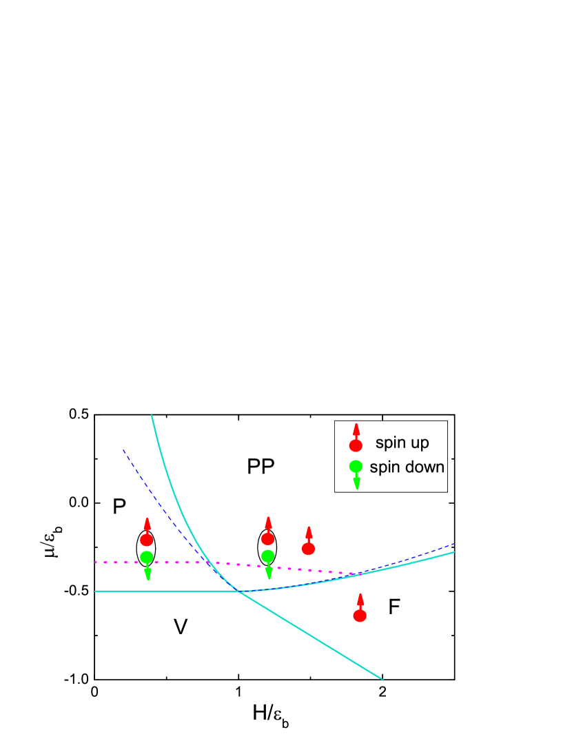
Figure 1: (Color online)Phase diagram in $\mu-H$ plane: The phase boundaries are represented by solid lines. The $V-F$, $V-P$ boundaries are given in Eq.(5), and $F-PP$ and $P-PP$ boundaries are numerical plot of Eq. (3) and (4). The blue-dashed lines are the extrapolation of the phase boundaries Eq. (6) and (7) in the strongly coupling regime, which is the region below the purple dotted lines, given by $\sqrt{\tilde{\mu}+1/2}\sim 1$, and $\sqrt{\tilde{\mu}+h/2}\sim 1$. Quantum phase transition occurs as the driving parameters $\tilde{\mu}$ and $h$ cross the phase boundaries at zero temperature. The $\mu-h$ phase diagram was found from the ground state Fredholm equations in Orso ; Hu .

II II. Exact $T=0$ phase boundaries of attractive 1D Fermi gas

The Hamiltonian of a 1D Fermi gas with attractive $\delta$-function interaction is ${\cal K}={\cal H}-\mu N-hM$,

$${\cal H}=\frac{\hbar^{2}}{2m}\int{\rm d}x\left(\partial\psi^{\dagger}_{\sigma}\partial\psi_{\sigma}+c\psi^{\dagger}_{\uparrow}\psi^{\dagger}_{\downarrow}\psi_{\downarrow}\psi_{\uparrow}\right),$$ (1)

$N=\sum_{\sigma}\int{\rm d}x\psi^{\dagger}_{\sigma}\psi_{\sigma}$, $M=\frac{1}{2}\int{\rm d}x(\psi^{\dagger}_{\uparrow}\psi_{\uparrow}-\psi^{\dagger}_{\downarrow}\psi_{\downarrow})$, where $\sigma=\uparrow,\downarrow$ are the spin labels. $c$ has the dimension of (length)^-1. Because of attractive interaction, i.e. $c<0$, fermions with opposite spin can form a bound pair with binding energy $\varepsilon_{b}=\hbar^{2}c^{2}/4m$ and spatial extent $|c|^{-1}$. The parameter $\gamma=|c|/n$, which is the ratio between inter-particle spacing ($1/n)$ and width of the bound pair $|c|^{-1}$, divides the system into a regime of tightly bound pairs ($\gamma<-1$), and overlapping pairs ($-1<\gamma<0$). For systems with spin polarization, both bound pairs and unpaired fermions coexist. The equilibration between them, even for very small polarization, will make $h\sim\varepsilon_{b}$; and we shall later consider temperature regimes, $T<\varepsilon_{b},h$. For our discussions, it is convenient to use dimensionless quantities where energy and length are measured is in units of $\varepsilon_{b}$ and $c^{-1}$ respectively. We shall define $\tilde{\mu}\equiv\mu/\varepsilon_{b}$, $h\equiv H/\varepsilon_{b}$, $t\equiv T/\varepsilon_{b}$, $\tilde{n}\equiv n/|c|=\gamma^{-1}$, $\tilde{p}\equiv P/|c\varepsilon_{b}|$. From the BA equation, it can be shown that the strongly coupling limit $\gamma>>1$ corresponds to $\sqrt{\tilde{\mu}+h/2}<<1$ and $\sqrt{\tilde{\mu}+{1}/2}<<1$.

1D interacting Fermi gas with contact interaction is one of the most important exactly solvable quantum many-body systems, and the associating BA solution is among the greatest achievements in mathematical physics Yang-a . This model contains only one interaction parameter $c$. Yet it is enough to generate a great diversity of intricate collective phenomena, including spin-charge separation (for $c>0$) and oscillatory paring $(c<0)$. The BA solution, however, is formidable. Despite the considerable analytical effort in deriving the thermodynamic Bethe Ansatz (TBA) equations that describe the thermodynamics of the system, they have only been solved numerically in most cases Mueller ; Kakashvili ; Hulet and analytically for special coupling regimes Guan ; Erhai .

The $T=0$ phase diagram has been worked out by Orso Orso and by others Hu ; Guan ; Wadati using BA equations, which describe the ground state within a canonical ensemble Yang-Gaudin . Here we study the phase diagram by taking the $T\rightarrow 0$ limit of the TBA equations Takahashi in a grand canonical ensemble Y-Y and present analytical critical fields in $\mu-H$ plane. The phase diagram is shown in Figure  1. It consists of four phases: vacuum $(V)$, fully paired phase $(P)$, ferromagnetic phase $(F)$, and partially paired $(PP)$ or ($FFLO$-like) phase. The phase boundaries between $V-F$, $V-P$, $F-PP$, and $P-PP$ are denoted as $\mu_{c1}$ to $\mu_{c4}$ respectively. The quantum phase transitions in the 1D attractive Fermi gas are determined by the following dressed energy equations Takahashi ; Guan

$$\epsilon^{\rm b}(\Lambda) = 2\left(\Lambda^{2}-\mu-\frac{c^{2}}{4}\right)-\int_{-B}^{B}a_{2}(\Lambda-\Lambda^{\prime}){\epsilon^{\rm b}}(\Lambda^{\prime})d\Lambda^{\prime}$$

$$-\int_{-Q}^{Q}a_{1}(\Lambda-k){\epsilon^{\rm u}}(k)dk,$$

$$\epsilon^{\rm u}(k) = \left(k^{2}-\mu-\frac{H}{2}\right)-\int_{-B}^{B}a_{1}(k-\Lambda){\epsilon^{\rm b}}(\Lambda)d\Lambda$$ (2)

which are obtained from the TBA equations in the limit $T\to 0$. In the above equations $a_{m}(\lambda)=\frac{1}{2\pi}\frac{m|c|}{(mc/2)^{2}+\lambda^{2}}$. The dressed energy $\epsilon^{\rm b}(\Lambda)\leq 0$ ($\epsilon^{\rm u}(k)\leq 0$) for $|\Lambda|\leq B$ ($|k|\leq Q$) correspond to the occupied states. The positive part of $\epsilon^{\rm b}$ ($\epsilon^{\rm u}$) corresponds to the unoccupied states. The integration boundaries $B$ and $Q$ characterize the Fermi surfaces for bound pairs and unpaired fermions, respectively. The phase boundary can be worked out by analyzing the band fillings with respect to the field $H$ and the chemical potential $\mu$ at $T=0$. The ($V-F$) phase boundary is determined by the conditions $\epsilon^{\rm u}(0)\leq 0$ and $\epsilon^{\rm b}(0)>0$, which gives $\mu_{c1}=-h/2$. Whereas the ($V-P$) phase boundary is determined by the conditions $\epsilon^{u}(0)>0$ and $\epsilon^{b}(0)\leq 0$, which gives $\mu_{c2}=-1/2$.

The ($F-PP$) phase boundary is determined by $\epsilon^{\rm b}(0)\leq 0$ and $\epsilon^{\rm u}(\pm Q)=0$ which gives the critical field in dimensionless units by

$$\mu_{c3}=-\frac{1}{2}-\frac{1}{2\pi}\left[Q-(2\mu_{c3}+h+1)\arctan{Q}\right]$$ (3)

with $Q=\sqrt{2\mu_{c3}+h}$ footnote , see the solid ($F-PP$) phase line $\mu_{3}$ in Fig. 1. The most complicated phase boundary indicating the quantum phase transition ($P-PP$) from fully paired phase into the partially polarized phase may be determined by the conditions $\epsilon^{\rm u}(0)\leq 0$ and $\epsilon^{\rm b}(\pm B)=0$, i.e. the Fermi sea of unpaired fermion starts filling. Thus we have

$$\mu_{c4} = -\frac{h}{2}-\frac{4}{\pi}\int_{-\tilde{B}}^{\tilde{B}}\frac{\epsilon^{b}(\Lambda)d\Lambda}{1+4\Lambda^{2}}$$

$$\epsilon^{b}(\Lambda) = 2\Lambda^{2}-\mu_{c4}-\frac{1}{2}-\frac{1}{\pi}\int_{-\tilde{B}}^{\tilde{B}}\frac{\epsilon^{b}(\Lambda^{\prime})d\Lambda^{\prime}}{1+(\Lambda-\Lambda^{\prime})^{2}}$$

$$\tilde{B}^{2} = \frac{1}{2}\left(\mu_{c4}+\frac{1}{2}\right)+\frac{1}{2\pi}\int_{-\tilde{B}}^{\tilde{B}}\frac{\epsilon^{b}(\Lambda)d\Lambda}{1+(\tilde{B}-\Lambda)^{2}},$$ (4)

which provide exact critical field $\mu_{c4}$, see solid $P-PP$ line in Fig. 1. In order to study quantum criticality of strongly Fermi gas, close forms of critical fields are essential to determine scaling functions of thermodynamical properties. They are

$$\mu_{c1} = -\frac{h}{2};\,\,\,\,\mu_{c2}=-\frac{1}{2},$$ (5)

$$\mu_{c3} = -\frac{1}{2}\left(1-\frac{2}{3\pi}(h-1)^{\frac{3}{2}}-\frac{2}{3\pi^{2}}(h-1)^{2}\right),$$ (6)

$$\mu_{c4} = -\frac{h}{2}+\frac{4}{3\pi}(1-h)^{\frac{3}{2}}+\frac{3}{2\pi^{2}}(1-h)^{2}.$$ (7)

While Eq.(5) applies to all regimes, Eq.(6) and (7) are expressions in the strongly interacting regime, see the dashed lines in Fig. 1. The above critical fields (6) and (7) can be also obtained by converting the critical fields in the $h-n$ plane, which were found in Guan , into the $\mu-h$ plane.

III III. Equation of state

The lack of analytic solutions of the TBA equation has made calculations of physical properties cumbersome, severely limits ones ability to make predictions and to identify the physical origin of observed effects. While bosonization or Luttinger liquid theory can provide qualitative information of low temperature properties, they do not give equation of states and are accurate only within a limited range of temperature. The construction of more transparent solutions for thermodynamic functions becomes even more desirable in view of the recent progress in the experiments on 1D Fermi gas with attractive interaction, as well as the successes in deducing equation of state of Fermi gases from non-uniform density data. A close analytic form of thermodynamic functions will certainly make comparisons between theory and experiments easier.

The thermodynamics of this system has been studied analytically Guan ; Erhai and numerically Mueller ; Kakashvili ; Hulet using TBA equations. Ref. Guan studies the free energy at very low temperatures for the spin balanced case, and shows that it is well described by Tomonaga-Luttinger liquid theory. The Luttinger description, however, is incapable of describing quantum criticality for it does not contain the critical fluctuations. TBA equations are a complex set of equations in terms of the so-called “dressed energies” of bound pairs, unpaired fermions, and spin wave bound states. In Ref.Erhai , these equations were recasted into coupled equations of thermodynamic quantities, obtained by approximating the dressed energies to the lowest order in $t$, and taking the $T|c|\rightarrow\infty$ limit for the so-called “string contributions” which describe the effect of the spin waves. To describe quantum criticality accurately, however, higher order terms in $t$ in the dressed energy have to be retained. (See footnote note below). From the TBA equations Takahashi ; Guan , it can be shown that the dressed energies can be calculated in terms of plolylog functions

$$\epsilon^{\rm b}(k)=2(\frac{h^{2}}{2m}k^{2}-\mu-\frac{\hbar^{2}}{2m}\frac{c^{2}}{4})+\frac{|c|p^{b}}{c^{2}+k^{2}}$$

$$+\frac{T^{\frac{5}{2}}}{4\sqrt{2\pi}|c|^{3}}\mathrm{Li}_{\frac{5}{2}}\left(-e^{\frac{A_{0}^{\rm b}}{T}}\right)+\frac{|c|p^{u}}{\frac{c^{2}}{4}+k^{2}}$$

$$+\frac{T^{\frac{5}{2}}}{\sqrt{\pi}|c|^{3}}\mathrm{Li}_{\frac{5}{2}}\left(-e^{\frac{A_{0}^{\rm u}}{T}}\right)+O\left(\frac{1}{|c|^{4}}\right)$$ (8)

$$\epsilon^{\rm u}(k)=\frac{\hbar^{2}}{2m}k^{2}-\mu-\frac{H}{2}+\frac{p^{\rm b}}{2}\frac{|c|}{\frac{c^{2}}{4}+k^{2}}$$

$$+\frac{\sqrt{2}}{\sqrt{\pi}}\frac{1}{|c|^{3}}\frac{T^{\frac{5}{2}}}{\left(\frac{\hbar^{2}}{2m}\right)^{\frac{3}{2}}}\mathrm{Li}_{\frac{5}{2}}\left(-e^{\frac{A_{0}^{b}}{T}}\right)$$

$$-Te^{-\frac{H}{T}}e^{-K}I_{0}(K)+O\left(\frac{1}{c^{4}},e^{\frac{-2H}{T}}\right)$$ (9)

where

$$A_{0}^{\rm b} \approx 2\mu+\frac{c^{2}}{2}-\frac{p^{\rm b}}{|c|}-\frac{4p^{\rm u}}{|c|},$$

$$A_{0}^{\rm u} \approx \mu+\frac{H}{2}-\frac{2p^{\rm b}}{|c|}-\frac{4p^{\rm u}}{|c|}$$

and $Li_{s}(z)=\sum_{k=1}^{\infty}z^{k}/k^{s}$ is the polylog function, $K=-\frac{t^{\frac{1}{2}}}{\sqrt{2\pi}}f_{3/2}^{u}$, and $I_{0}(x)=\sum_{k=0}^{\infty}\frac{1}{(k!)^{2}}(\frac{x}{2})^{2k}$ comes from the so-called “string” or spin wave contributions. The above result depends on an important observation that the convolution terms in the TBA equations converge quickly as $\epsilon^{\rm b}(k)$ and $\epsilon^{\rm u}(k)$ become greater than zero at low temperatures. Using the above asymptotic of dressed energies we can calculate pressure in a straightforward way. Substituting above dressed energies into the pressure per unit length $p=p^{b}+p^{u}$

$$p^{b} = \frac{T}{\pi}\int_{-\infty}^{\infty}dk\ln(1+\mathrm{e}^{-\epsilon^{\rm b}(k)/{T}})$$

$$P^{u} = \frac{T}{2\pi}\int_{-\infty}^{\infty}dk\ln(1+\mathrm{e}^{-\epsilon^{\rm u}(k)/{T}}),$$ (10)

and taking integration by part, thus we obtain the following dimensionless form of the pressure of the system as

$$\tilde{p}(t,\tilde{\mu},h)\equiv p/(|c|\varepsilon_{b})=\tilde{p}^{b}+\tilde{p}^{u},$$ (11)

where $\tilde{p}^{b}$ and $\tilde{p}^{u}$ can be interpreted as the pressure of the bound pair and unpaired fermions, and are coupled through the following set of equations,

$$\tilde{p}^{b} = -\frac{t^{\frac{3}{2}}}{2\sqrt{\pi}}F_{3/2}^{b}\left[1+\frac{\tilde{p}^{b}}{8}+2\tilde{p}^{u}\right]+O(t^{4})$$ (12)

$$\tilde{p}^{u} = -\frac{t^{\frac{3}{2}}}{2\sqrt{2\pi}}F_{3/2}^{u}\left[1+2\tilde{p}^{b}\right]+O(t^{4})$$ (13)

$$\frac{X_{b}}{t} = \frac{\nu_{b}}{t}-\frac{\tilde{p}^{b}}{t}-\frac{4\tilde{p}^{u}}{t}-\frac{t^{\frac{3}{2}}}{\sqrt{\pi}}\left(\frac{1}{16}f_{5/2}^{b}+\sqrt{2}f_{5/2}^{u}\right)$$ (14)

$$\frac{X_{u}}{t} = \frac{\nu_{u}}{t}-\frac{2\tilde{p}^{b}}{t}-\frac{t^{\frac{3}{2}}}{2\sqrt{\pi}}f_{5/2}^{b}+e^{-\frac{h}{t}}e^{-K}I_{0}(K)$$ (15)

where the functions $F_{n}^{b}$, $F_{n}^{u}$, $f_{n}^{b}$, and $f_{n}^{u}$ are defined as

$$F_{n}^{b}\equiv Li_{n}\left(-e^{\frac{X_{b}}{t}}\right),\qquad F_{n}^{u}\equiv Li_{n}\left(-e^{\frac{X_{u}}{t}}\right)$$

$$f_{n}^{b}\equiv Li_{n}\left(-e^{\frac{\nu_{b}}{t}}\right),\qquad f_{n}^{u}\equiv Li_{n}\left(-e^{\frac{\nu_{u}}{t}}\right)$$ (16)

where $\nu_{b}\equiv 2{\tilde{\mu}}+1$, $\nu_{u}\equiv\tilde{\mu}+h/2$; $X_{b}$, $X_{u}$ are defined as in Eq.(14) and Eq.(15).

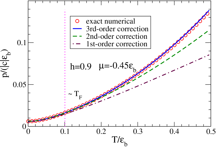
Figure 2: (Color online)Pressure vs temperature: Comparisons between the numerical results from Eq.(12) to (15) (represented by circles) with the analytical result from Eq. (17) up to the order $Y^{(u,b)}_{\frac{1}{2}}$ (1st order), $Y^{(u,b)}_{1}$ (2nd order) and $Y^{(u,b)}_{\frac{3}{2}}$ (3rd oder).

The derivation of Eq.(12) to (15) is very involved. That we present these equations is to prepare for the later discussions of the mathematical manipulation needed to extract the singularity near the quantum critical point. To solve these equations, one substitutes Eqs (14) and (15) into Eq.(12) and (13). This gives two coupled equations of $\tilde{p}^{b}$ and $\tilde{p}^{u}$, which can be solved by iteration. From Eqs (14) and (15), we can rewrite the functions $\mathrm{Li}_{\frac{3}{2}}\left(-e^{X_{b}/t}\right)$ and $\mathrm{Li}_{\frac{3}{2}}\left(-e^{X_{u}/t}\right)$ in terms of the function $f_{n}^{b}$ and $f_{n}^{u}$. After lengthy algebra, the pressures are given by $\tilde{p}=\sqrt{2}\tilde{p}^{\rm b}+\tilde{p}^{\rm u}$ with

$$\tilde{p}^{x} = -\frac{t^{\frac{3}{2}}}{2\sqrt{2\pi}}\left[f_{\frac{3}{2}}^{x}+t^{\frac{1}{2}}Y_{\frac{1}{2}}^{x}+tY_{1}^{x}+t^{\frac{3}{2}}Y^{x}_{\frac{3}{2}}+O(t^{2})\right].$$ (17)

where $x=b,u$ and $\left\{Y_{n}^{b}\right\}$ and $\left\{Y_{n}^{u}\right\}$ are given by

$$Y_{\frac{1}{2}}^{b} = \frac{1}{\sqrt{\pi}}f_{\frac{1}{2}}^{b}\left(\frac{1}{2}f_{\frac{3}{2}}^{b}+\sqrt{2}f_{\frac{3}{2}}^{u}\right),\qquad Y_{\frac{1}{2}}^{u}=\frac{1}{\sqrt{\pi}}f_{\frac{1}{2}}^{u}f_{\frac{3}{2}}^{b},$$

$$Y_{1}^{b} = \frac{1}{\pi}\left[f_{\frac{1}{2}}^{b}\left(\frac{1}{4}f_{\frac{1}{2}}^{b}f_{\frac{3}{2}}^{b}+\sqrt{2}f_{\frac{1}{2}}^{u}f_{\frac{3}{2}}^{b}+\frac{1}{\sqrt{2}}f_{\frac{1}{2}}^{b}f_{\frac{3}{2}}^{u}\right)\right.$$

$$\left.+f_{-\frac{1}{2}}^{b}\left(\left(f_{\frac{3}{2}}^{u}\right)^{2}+\frac{1}{8}\left(f_{\frac{3}{2}}^{b}\right)^{2}+\frac{1}{\sqrt{2}}f_{\frac{3}{2}}^{b}f_{\frac{3}{2}}^{u}\right)\right],$$

$$Y_{1}^{u} = \frac{1}{\pi}\left[\sqrt{2}f_{\frac{1}{2}}^{b}f_{\frac{1}{2}}^{u}f_{\frac{3}{2}}^{u}+\frac{1}{2}f_{\frac{1}{2}}^{b}f_{\frac{1}{2}}^{u}f_{\frac{3}{2}}^{b}+\frac{1}{2}\left(f_{\frac{3}{2}}^{b}\right)^{2}f_{-\frac{1}{2}}^{u}\right].$$ (18)

The expressions of $Y^{b}_{\frac{3}{2}}$ and $Y^{u}_{\frac{3}{2}}$ are given in Appendix. The accuracy of Eq.(17) is shown in Figure 2, where the result of the expansion is compared with the numerical solution of the recast TBA equations. Eq.(12) to (15) served as equation of state (represented by circles). The vertical dotted line represents the Fermi temperature $T_{F}$ in the Rice experiment in ref. Hulet , where $T_{F}/\epsilon_{b}\sim 0.1$. Figure 2 shows that for $t<0.1$, (corresponds to $T<T_{F}$ in Hulet ), the pressure is accurately given by the first order correction in Eq.(17) (to about 1$\%$). At higher temperatures, higher order terms are needed. It is worth noting that by including terms up to third order, Eq.(17) agree essentially with the exact result for $t>0,5$.

Furthermore, if defining

$$\tilde{p}^{u}_{o} \equiv -\frac{t^{\frac{3}{2}}}{2\sqrt{2\pi}}f_{\frac{3}{2}}^{u},\qquad\tilde{p}^{b}_{o}\equiv-\frac{t^{\frac{3}{2}}}{2\sqrt{\pi}}f_{\frac{3}{2}}^{b},$$

$$\tilde{n}^{(b,u)}_{o} = \frac{\partial\tilde{p}^{(b,u)}_{o}}{\partial\tilde{\mu}^{(b,u)}},\qquad\tilde{\kappa}^{(b,u)}_{o}=\frac{\partial\tilde{n}^{(u,n)}_{o}}{\partial\tilde{\mu}^{(b,u)}},$$ (19)

up to the order of $Y^{(u,b)}_{1}$, we can rewrite the pressure (17) as

$$\tilde{p}^{b} \approx \tilde{p}_{o}^{b}-\tilde{n}_{o}^{b}\left(\tilde{p}^{b}_{o}+4\tilde{p}_{o}^{u}\right)+\tilde{n}_{o}^{b}\left(\tilde{n}_{o}^{b}\tilde{p}^{b}_{o}+8\tilde{n}_{o}^{u}\tilde{p}_{o}^{b}+4\tilde{n}_{o}^{b}\tilde{p}^{u}_{o}\right)$$

$$+\tilde{k}_{o}^{b}\left(8(\tilde{p}^{u}_{o})^{2}+\frac{1}{2}(\tilde{p}^{b}_{o})^{2}+4\tilde{p}^{b}_{o}\tilde{p}^{u}_{o}\right),$$

$$\tilde{p}^{u} \approx \tilde{p}_{o}^{b}-2\tilde{n}_{o}^{u}\tilde{p}_{o}^{b}+8\tilde{n}_{0}^{b}\tilde{n}_{o}^{u}\tilde{p}^{u}_{o}+2\tilde{n}_{o}^{b}\tilde{n}_{o}^{u}\tilde{p}_{o}^{b}+2\tilde{k}_{o}^{b}(\tilde{p}^{u}_{o})^{2}$$ (20)

which give insight into understanding cluster-cluster effect. From these analytical result of pressures, we see that the bound pairs interfere with each other and with excess fermions. The $Y$-terms in Eq.(17) can be viewed as interactions of boson-boson and boson-fermion clusters of increasingly size. We find that The pressure Eq. (17) can reach $95\%$ accuracy for $T/\varepsilon_{b}=0.2$ by including upto the $Y^{x}_{1}$ terms, and has less than $1\%$ error if one includes the $Y_{\frac{3}{2}}^{x}$ terms, see Figure 2.

Finally, we note that in the limit $|c|\rightarrow\infty$, the pressure (10) gives the following equation of state $P(T,\mu,H)=\sqrt{2}{\cal P}(2\mu_{b})+{\cal P}(\mu_{u})$ with $T\ll\mu_{b},\,\mu_{u}$, where

$${\cal P}(x)\approx\frac{2\sqrt{2}}{3\pi}\sqrt{\frac{m}{\hbar^{2}}}x^{\frac{3}{2}}\left(1+\frac{\pi^{2}}{8}\left(\frac{T}{x}\right)^{2}+\frac{7\pi^{4}}{640}\left(\frac{T}{x}\right)^{4}\right)$$ (21)

is the pressure of a 1D Fermi gas with mass $m$. In this limit, for fixed total density $n$, the effective chemical potentials for pairs and unpaired fermions are given by

$$\mu_{\rm b}\approx\frac{\hbar^{2}n^{2}\pi^{2}}{2m}\frac{(1-P)^{2}}{16},$$ (22)

$$\mu_{\rm u}\approx\frac{\hbar^{2}n^{2}\pi^{2}}{2m}P^{2}.$$ (23)

Where $P=(N_{\uparrow}-N_{\downarrow})/(N_{\uparrow}-N_{\downarrow})$ is the polarization. This result reflects the fact that the system reduces to a mixture of hard core boson (mass $2m$) and a gas of unpaired fermions (mass $m$) in this limit. Since hard core bosons in 1D behaves like fermions, the thermodynamics of the system is that of a mixture of two Fermi gases with mass $2m$ and $m$.

IV IV. Quantum Criticality

Quantum critical behaviors are reflected in the singularities in thermodynamic quantities such as density $\tilde{n}=n/|c|$, compressibility $\tilde{\kappa}=\partial\tilde{n}/\partial\tilde{\mu}$, and magnetization $\tilde{M}=M/|c|$, which are derivatives of pressure $p$ with respect to $\mu$ and $h$. Such singularities, however, cannot be obtained by directly differentiating the expansion Eq.(17). The reason is that even though Eq.(17) gives highly accurate value for the pressure with a few terms, all higher order terms which contribute insignificantly to the pressure have singularities when differentiated with respect to $\mu$. To account for these singular structures, say, in the density, one must first differentiate Eq.(12)-(15) with respect to $\tilde{\mu}$ to obtained coupled equations of $\partial\tilde{p}^{x}/\partial\tilde{\mu}$ and then solves for these quantities by iteration. Quantum phase transition occurs as the driving parameters $\tilde{\mu}$ and $\tilde{h}$ cross the phase bounaries at zero temperature. At very low temperatures, $T\ll\varepsilon_{b}$ (Boltzmann’s constant $k_{B}=1$), the thermodynamics of the 1D FFLO like phase is governed by the linearly dispersing phonon modes, i.e., the long wavelength density fluctuations of the two weakly coupled gases. In this low temperature regime, spin strings are suppressed. The suppression of spin fluctuations leads to a universality class of a two-component TLL in the gapless phase of FFLO, where the charge bound states form hard-core composite bosons. The leading low temperature corrections to the free energy give Guan ; Erhai

$$f\approx f_{0}-\frac{\pi T^{2}}{6\hbar}\left(\frac{1}{v_{b}}+\frac{1}{v_{u}}\right).$$ (24)

Here $f_{0}$ is the ground state energy and $v_{b,u}$ are the sound velocities of pairs and unpaired fermions, i.e.

$$v_{\rm b} \approx \frac{v_{\rm F}(1-P)}{4}\left(1+\frac{(1-P)}{|\gamma|}+\frac{4P}{|\gamma|}\right),$$

$$v_{\rm u} \approx v_{\rm F}P\left(1+\frac{4(1-P)}{|\gamma|}\right).$$ (25)

Here the Fermi velocity is $v_{\rm F}=\hbar\pi n/m$. The TLL maintains below the cross-over temperature at which the relation of the linear temperature-dependent entropy (or specific) heat breaks down. The equation of state Eq.(12) to (15) and the TLL nature (24) allow ones to quantitatively investigate quantum criticality of the Fermi gas, see Fig.  3.

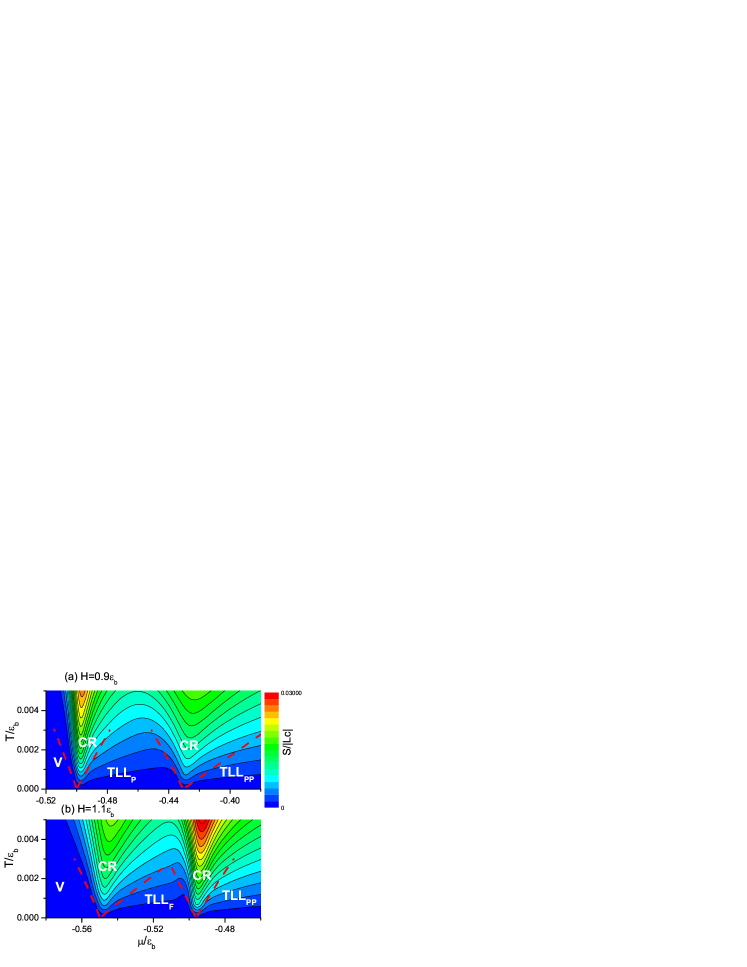
Figure 3: (Color online)Contour plot entropy $S$ vs chemical potential $\mu$ from Eq. Eq.(12) to (15) for different values of effective magnetic field note-figure . The cross-over temperatures separated TLL phases from quantum critical regimes are determined from the breakdown of linear temperature-dependent entropy. Here $TLL_{F}$ stands for the Tomonaga-Luttinger liquid of the single component of unpaired fermions. While $TLL_{P}$ stands for the TLL of pairs and $TLL_{PP}$ for the two-component TLL of FLLO-like states. The left-most dashed line separates quasi-classical regime from the quantum critical regime. The cross-over temperatures merge at critical points as $T\to 0$.

Using the standard thermodynamic relations, we can derive close forms of density, magnetization, compressibility which allow ones to capture universal low temperature thermodynamics of the Fermi gas as well as critical phenomena. Without losing generality, we can safely ignore spin wave contribution at quantum criticality due to its exponentially small contribution as $T\to 0$. For our convenience in calculating the thermodynamical properties, we denote

$$f_{n}^{A_{b}} \equiv Li_{n}\left(-e^{\frac{A_{b}}{t}}\right),\,\frac{A_{b}}{t}=\frac{\nu_{b}}{t}+\frac{t^{\frac{1}{2}}}{\sqrt{\pi}}\left(\frac{1}{2}f_{\frac{3}{2}}^{b}+\sqrt{2}f_{\frac{3}{2}}^{u}\right),$$

$$f_{n}^{A_{u}} \equiv Li_{n}\left(-e^{\frac{A_{u}}{t}}\right),\,\,\,\frac{A_{u}}{t}=\frac{\nu_{u}}{t}+\frac{t^{\frac{1}{2}}}{\sqrt{\pi}}f_{\frac{3}{2}}^{b}.$$ (26)

From the equations Eq.(12)-(15), We derived the total density $\tilde{n}=(\tilde{n}_{\uparrow}+\tilde{n}_{\downarrow})$

$$\tilde{n}=-\frac{\sqrt{t}}{\sqrt{\pi}\Delta}\left\{\frac{1}{2\sqrt{2}}f_{\frac{1}{2}}^{A_{u}}\left[1+\frac{3\sqrt{t}}{2\sqrt{\pi}}f_{\frac{1}{2}}^{A_{b}}-\frac{47t^{\frac{3}{2}}}{16\sqrt{\pi}}f_{\frac{3}{2}}^{A_{b}}\right]\right.$$

$$\left.+f_{\frac{1}{2}}^{A_{b}}\left[1+\frac{\sqrt{t}}{\sqrt{2\pi}}f_{\frac{1}{2}}^{A_{u}}-\frac{t^{\frac{3}{2}}}{\sqrt{\pi}}\left(\frac{1}{8}f_{\frac{3}{2}}^{A_{b}}+\frac{3\sqrt{2}}{2}f_{\frac{3}{2}}^{A_{u}}\right)\right]\right\}$$ (27)

with

$$\Delta = 1-\frac{\sqrt{t}}{2\sqrt{\pi}}f_{\frac{1}{2}}^{A_{b}}-\frac{t\sqrt{2}}{\pi}f_{\frac{1}{2}}^{A_{b}}f_{\frac{1}{2}}^{A_{u}}+\frac{t^{\frac{3}{2}}}{16\sqrt{\pi}}f_{\frac{3}{2}}^{A_{b}}.$$ (28)

The density in dimensionless scale naturally services as the dimensionless equation of state which contain two free-fermion-like densities with singular behaviour near different critical points. The interaction binding energy rescales temperature. This close form of equation of state is very convenient to make fitting of experimental finite temperature density profiles of the 1D trapped gas within local density approximation, see Hulet ; note-figure .

Similarly, magnetization $\tilde{M}=(\tilde{n}_{\uparrow}-\tilde{n}_{\downarrow})/2$

$$\tilde{M} = -\frac{\sqrt{t}}{2\sqrt{\pi}\Delta}\left\{\frac{1}{2\sqrt{2}}f_{1/2}^{A_{u}}\left[1-\frac{\sqrt{t}}{2\sqrt{\pi}}f_{1/2}^{A_{b}}-\frac{31t^{\frac{3}{2}}}{16\sqrt{\pi}}f_{3/2}^{A_{b}}\right]\right.$$

$$\left.+\frac{\sqrt{t}}{\sqrt{2\pi}}f_{1/2}^{A_{b}}\left[f_{1/2}^{A_{u}}-tf_{\frac{3}{2}}^{A_{u}}\right]\right\};$$

susceptibility $\tilde{\chi}=\chi\varepsilon_{b}/|c|$ with $\chi=\partial M/\partial H$

$$\tilde{\chi} = -\frac{1}{8\sqrt{2\pi}\Delta^{3}}\left\{\frac{1}{\sqrt{t}}f_{-1/2}^{A_{u}}\left[1+\frac{3\sqrt{t}}{2\sqrt{\pi}}f_{1/2}^{A_{b}}+\frac{2\sqrt{2}t}{\pi}f_{1/2}^{A_{b}}f_{1/2}^{A_{u}}\right]\right.$$ (29)

$$\left.+\frac{2\sqrt{2}\sqrt{t}}{\pi}f_{-1/2}^{A_{b}}\left(f_{1/2}^{A_{u}}\right)^{2}\right\};$$

and compressibility $\tilde{\kappa}=\kappa\varepsilon_{b}/|c|$ with $\kappa=\partial n/\partial\mu$

$$\tilde{\kappa} = -\frac{1}{\sqrt{\pi}\Delta^{3}}\left\{\frac{1}{2\sqrt{2}\sqrt{t}}f_{-1/2}^{A_{u}}\left[1-\frac{5\sqrt{t}}{2\sqrt{\pi}}f_{1/2}^{A_{b}}-\frac{t}{4\pi}\left(f_{1/2}^{A_{b}}\right)^{2}\right]\right.$$ (30)

$$\left.+\frac{2}{\sqrt{t}}f_{-1/2}^{A_{b}}\left[1-\frac{\sqrt{t}}{2\sqrt{2\pi}}f_{1/2}^{A_{u}}-\frac{t}{4\pi}\left(f_{1/2}^{A_{u}}\right)^{2}\right]\right\}$$

can be derived in a systematic way.

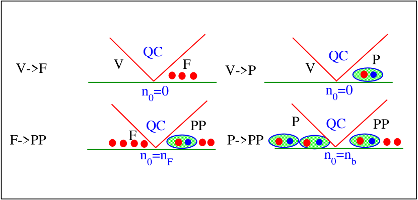
Figure 4: (Color online)Schematic illustration of universal critical phenomena near critical points for the 1D strongly attractive Femi gas, see Eq. (40). The density of bound pairs (excess fermions) become a regular part as the background meanwhile the one of excess fermions (bound pairs) become a singular part. However, there is no back ground density for the phase transition from vacuum into the fully-paired or fully-polarized phase, i.e. $V\to F$ or $V-P$.

Quantum criticality describes strongly coupled thermal and quantum fluctuations of matter as quantum phase transitions take place at zero temperature. Such quantum phase transitions are uniquely characterized by the critical exponents depending only on the dimensionality and the symmetry of the system. Here we show that scaling functions at quantum criticality can be calculated from the above close forms of thermodynamical properties. Near the critical points, we expand thermodynamical properties in the limit $|\mu-\mu_{c}|\ll 1$. For the quantum critical regime, i.e. $T>|\mu-\mu_{c}|$, we find that the thermodynamical properties of the Fermi liquid of bound pairs (excess fermions) become a regular part as the background meanwhile the ones of the Fermi liquid of excess fermions (bound pairs) become a singular part. Near the $T=0$ phase boundaries, we find that $\tilde{n}$ and $\tilde{M}$ have universal scaling forms

$$(V{\rm-}F) \,\,\,\,\,\,\tilde{n}\approx-\frac{\sqrt{t}}{2\sqrt{2\pi}}Li_{\frac{1}{2}}\left(-e^{\frac{(\tilde{\mu}-\mu_{c1})}{t}}\right)\hskip 36.135pt$$ (31)

$$\tilde{M}\approx-\frac{\sqrt{t}}{4\sqrt{2\pi}}Li_{\frac{1}{2}}\left(-e^{\frac{(\tilde{\mu}-\mu_{c1})}{t}}\right)\hskip 36.135pt$$ (32)

$$(F{\rm-}PP) \,\,\tilde{n}\approx n_{o3}-\lambda_{1}\sqrt{t}Li_{\frac{1}{2}}\left(-e^{\frac{2(\tilde{\mu}-\mu_{c3})}{t}}\right)\hskip 36.135pt$$ (33)

$$\tilde{M}\approx M_{o}+\lambda_{3}\sqrt{t}Li_{\frac{1}{2}}\left(-e^{\frac{2(\tilde{\mu}-\mu_{c3})}{t}}\right)\ \hskip 36.135pt$$ (34)

$$(V{\rm-}P)\hskip 14.45377pt\,\,\tilde{n}\approx-\frac{\sqrt{t}}{\sqrt{\pi}}Li_{\frac{1}{2}}\left(-e^{\frac{2(\tilde{\mu}-\mu_{c2})}{t}}\right)\hskip 36.135pt$$ (35)

$$\tilde{M}\approx\frac{t}{2\sqrt{2}\pi}Li_{\frac{1}{2}}\left(-e^{\frac{2(\tilde{\mu}-\mu_{c2})}{t}}\right)Li_{\frac{1}{2}}\left(-e^{\frac{(h-1)}{2t}}\right)\sim 0$$ (36)

$$(P{\rm-}PP)\hskip 14.45377pt\,\,\tilde{n}\approx n_{o4}-\lambda_{2}\sqrt{t}Li_{\frac{1}{2}}\left(-e^{\frac{(\tilde{\mu}-\mu_{c4})}{t}}\right)\hskip 21.68121pt$$ (37)

$$\,\,\tilde{M}\approx-\frac{\sqrt{t}}{4\sqrt{2\pi}}Li_{\frac{1}{2}}\left(-e^{\frac{(\tilde{\mu}-\mu_{c}4)}{t}}\right)\left(1-\frac{4\sqrt{b}}{\pi}\right)\hskip 21.68121pt$$ (38)

where $n_{o3},n_{o4},a,b,M_{o}$ are constants independent of $\tilde{\mu}$ and $t$. The expressions are given by

$$n_{o3} = \frac{\sqrt{a}}{2\pi},\qquad\lambda_{1}=\frac{1}{\sqrt{\pi}}\left(1-\frac{2\sqrt{a}}{\pi}+\frac{a}{\pi^{2}}\right),$$

$$a = (h-1)(1+\frac{2}{3\pi}\sqrt{h-1}),$$

$$n_{o4} = \frac{2\sqrt{b}}{\pi}\left(1-\frac{\sqrt{b}}{\pi}+\frac{b}{\pi^{2}}\right),$$

$$\lambda_{2} = \frac{1}{2\sqrt{2\pi}}\left(1-\frac{8\sqrt{b}}{\pi}+\frac{17b}{\pi^{2}}\right),$$

$$b = (1-h)(1+\frac{2}{\pi}\sqrt{1-h}),$$

$$M_{o} = \frac{\sqrt{a}}{4\pi},\,\,\lambda_{3}=\frac{\sqrt{a}}{2\pi^{\frac{3}{2}}}\left(1-\frac{\sqrt{a}}{\pi}-\frac{2a}{3}\right).$$ (39)

In the above equations $n_{o3}$ and $n_{o4}$ are the background densities near the critical points $\mu_{3}$ and $\mu_{4}$, respectively. At quantum criticality, the above densities can be casted into a universal scaling form, e.g. ZhouHo ; Fisher ; Sachdev ; Mueller2 ,

$$n(\mu,T)=n_{0}+T^{\frac{d}{z}+1-\frac{1}{\nu z}}{\cal G}\left(\frac{\mu-\mu_{c}}{T^{\frac{1}{\nu z}}}\right),$$ (40)

Where the dynamic exponent $z=2$ and correlation exponent $\nu=1/2$ can be read off the scaling functions within the expressions Eq.(31) to (38) from which physical origin of quantum criticality is conceivable.

Eq.(31) to (38) has a simple interpretation. First of all, it is straightforward to work out the critical properties of a 1D free Fermi gas (single component), as well as for a mixture of two different Fermi gases. In the former case, the quantum phase transition (as a function of chemical potential) is from vacuum to Fermi gas, which we denote as type ${\bf(a)}$. In the two component case, if the two Fermi gases have different particle numbers, then there is a transition from vacuum to the majority component as a function of $\tilde{\mu}$ (for fixed $h$), i.e. type ${\bf(a)}$. There is also another transition from the majority component to a mixture, which we denote as type ${\bf(b)}$. Comparing Eq.(31) to (38) with the critical properties of Fermi gas mixtures, one notes that the transition $V-F$ and $V-P$ is that of type ${\bf(a)}$ where the “fermion mass” for the $V-F$ transition is $m$, and $2m$ for the $V-P$ transition. In the $V-P$ case, this is due to the fact that the tightly bound fermion pair acts like a hard core boson, which in turn acts as a fermion in 1D. In contrast, the transitions $F-PP$ and $P-PP$ are of type ${\bf(b)}$, where the Fermi gas mixture is made of particles with mass $m$ and $2m$. This critical phenomena is schematically illustrated in Fig . 4.

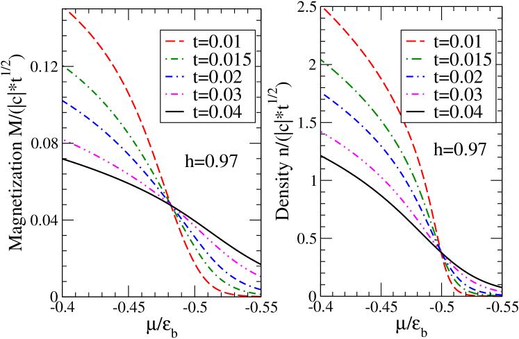
Figure 5: (Color online)Magnetization $M$ and density $n$ vs chemical potential $\mu$ at different temperatures. The intersections at the right and left panel give the phase boundaries of $V-P$ and $P-PP$ transition respectively.

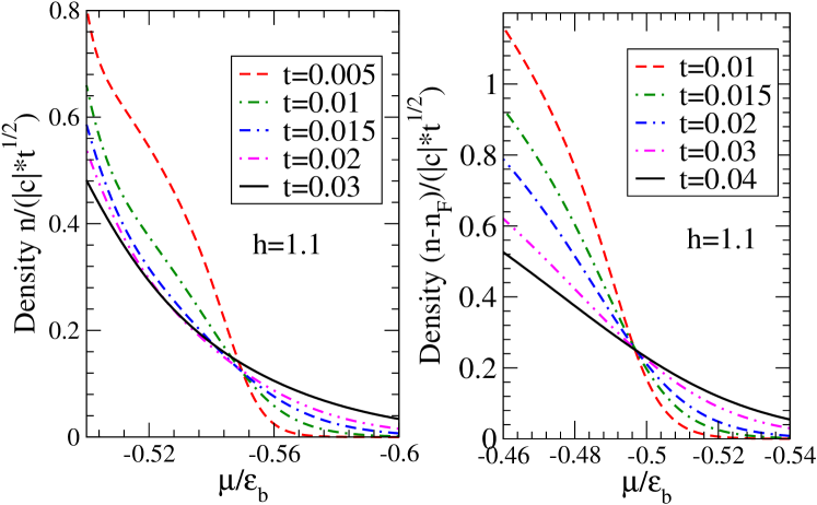
Figure 6: (Color online)Density vs chemical potential: The right panel shows the intersection of the density difference $(\tilde{n}-\tilde{n}_{F})/\sqrt{t}$ at different temperatures, which gives the $F-PP$ phase boundary. Here, we have $\tilde{n}_{F}=-\frac{\sqrt{t}}{2\sqrt{2\pi}}Li_{\frac{1}{2}}(-e^{A_{u}/t})$ with $A_{u}\approx\nu_{u}+t^{\frac{3}{2}}f_{3/2}^{b}/\sqrt{\pi}$. It becomes the density of a free fermion system in the vicinity of $F-PP$ phase boundary, i.e. $A_{u}$ reduces to $\nu_{u}$. The left panel shows the intersection of densities which gives the $V-F$ phase boundary. It also shows that the scaling form begins to fail for $t\geq 0.03$.

V V. Mapping out the $T=0$ phase diagram using quantum criticality

As pointed out in Ref.ZhouHo , the scaling property of the density near a quantum critical point enables one to determine the $T=0$ phase boundary of homogenous bulk systems from the non-uniform density profile of a trapped gas at $T>0$. All one needs to do is to plot the density profile $n(x)$ of the trapped gas as a function of local chemical potential $\mu(x)=\mu-V(x)$ at different temperatures, where $V(x)$ is the trapping potential. At low temperatures, these density curves will intersect at the same point. The chemical potential ($\mu_{c}$) associated with this intersection point is $T=0$ phase boundary. The existence of this intersection is due to the fact that the singular part of the density is a function of $(\mu-\mu_{c})/T$, as seen in Eq.(31) to Eq.(38). These intersections are seen in Fig. 5 to Fig.  6, which show the numerical solution of the recast TBA equations Eq.(12) to (15) for the $n$ and $M$ as a function of $\mu$ over a range of chemical potential much larger than the scaling region where Eq.(31) to Eq.(38) hold. They are equivalent to plotting the experimental density data in a manner mentioned above. The left and right panel of Fig.  5 show the $\tilde{\mu}$ dependence of $\tilde{M}$ and $\tilde{n}$ across the $V-PP$ phase boundaries (Eq.(38) and Eq.(35) ) respectively. In Fig.  6, the left panel shows $\tilde{n}$ vs $\tilde{\mu}$ across the $V-F$ phase boundary, Eq.(31). The right panel shows $\tilde{n}-\tilde{n}_{F}$ vs $\tilde{\mu}$ across the $F-PP$ phase boundary, Eq.(33). The intersections of these curves yield the critical value $\mu_{c}$ at $T=0$. In these figures, we displayed temperature variations from $t=0.01$ to $t=0.04$. The former corresponds to $T/T_{F}=0.1$ in the recent Rice set up, which is the temperature in the current Rice experiment Hulet .

In general, the slope of densities at the quantum criticality can be written as the following universal scaling form near the critical points:

$$\left(n(t,\mu)-n_{0}\right)t^{-1/2}=\lambda\sum_{m=0}^{\infty}c_{m}x^{m}$$ (41)

where $x=\frac{\mu-\mu_{c}}{t}$ and the coefficients $c_{m}=\frac{1}{m!}Li_{\frac{1}{2}-m}(-1)$. The intersection behaviour can accurately determine the temperature from the slops near the intersection point. For a given polarization (or say fixed polarization), the $\lambda$ becomes constant, (see, Eq.(31) to Eq.(38)). Thus the slops are uniquely fixed by temperatures. Perhaps this scaling behaviour is a good thermometry Mueller-note .

Finally, we would like to mention that similar plots can be constructed for compressibility across all phase boundaries, see Fig. 7. For compressibility, it is important (as stressed before) to include all higher order terms in Eq.(17), as they are all singular at criticality; and such inclusion can be achieved efficiently by taking derivatives of Eq (27) with respect to $\tilde{\mu}$ together with performing proper iteration via Eq.(12)-(15) . The expression of the critical behavior near various phase boundaries are given by

$$V{\rm-}F:\,\,\tilde{\kappa} \approx -\frac{1}{2\sqrt{2\pi t}}{\rm Li}_{-\frac{1}{2}}\left(-e^{\frac{(\tilde{\mu}-\mu_{c1})}{t}}\right)$$ (42)

$$F{\rm-}PP:\,\,\tilde{\kappa} \approx \kappa_{o3}-\frac{\lambda_{4}}{\sqrt{t}}{\rm Li}_{-\frac{1}{2}}\left(-e^{\frac{2(\tilde{\mu}-\mu_{c3})}{t}}\right)$$ (43)

$$V{\rm-}P:\,\,\tilde{\kappa} = -\frac{2}{\sqrt{\pi t}}{\rm Li}_{-\frac{1}{2}}\left(-e^{\frac{2(\tilde{\mu}-\mu_{c2})}{t}}\right)$$ (44)

$$P{\rm-}PP:\,\,\tilde{\kappa} = \kappa_{o4}-\frac{\lambda_{5}}{\sqrt{t}}{\rm Li}_{-\frac{1}{2}}\left(-e^{\frac{(\tilde{\mu}-\mu_{c4})}{t}}\right)$$ (45)

where $\kappa_{o3},\kappa_{o4},\lambda_{4},\lambda_{5}$ are given

$$\kappa_{o3} = \frac{1}{2\pi\sqrt{a}},\,\,\lambda_{4}=\frac{2}{\sqrt{\pi}}\left(1+\frac{\sqrt{a}}{2\pi}-\frac{a}{2\pi^{2}}\right)$$

$$\kappa_{o4} = \frac{2}{\pi\sqrt{b}}\left(1-\frac{3\sqrt{b}}{\pi}+\frac{6b}{\pi^{2}}\right),$$

$$\lambda_{5} = \frac{1}{2\sqrt{2\pi}}\left(1+\frac{2\sqrt{b}}{\pi}-\frac{10b}{\pi^{2}}\right).$$ (46)

The critical exponents $z=2$ and $\nu=1/2$ can be read off the universal scaling function

$$\kappa(\mu,T)=\kappa_{0}+T^{\frac{d}{z}+1-\frac{2}{\nu z}}{\cal F}\left(\frac{\mu-\mu_{c}}{T^{\frac{1}{\nu z}}}\right)$$ (47)

with an universal scaling function ${\cal F}(x)={\rm Li}_{-\frac{1}{2}}(x)$.

VI VI. Conclusion

We have studied the quantum critical phenomena of strongly attractive 1D Fermi gas via exact BA solution. We have obtained the equation of state with high precision from zero temperature up to the temperature scale of binding energy. From the equation of state, we have obtain the exact scaling form for density, compressibility, and spin susceptibility in the vicinity of the $T=0$ phase boundaries between different phases. These scaling forms illustrate the universal TLL signature and physical origin of quantum criticality. The excitations near various phase boundary is such that their critical behaviors are either described by that of free fermions and that mixtures of fermions with mass m and 2m.

Our exact results can help analyze the recent experiments on attractive 1D spin-imbalanced atomic Fermi gas Hulet . It can also help to verify the working of an algorithm for determining the $T=0$ phase boundary and quantum critical behavior based solely on measured density profile ZhouHo . The BA method proves to be a powerful tool to obtain exact results for quantum critical behavior. Further application of this method to other integrable systems including spinor gases may reveal new excitations and interesting physics.

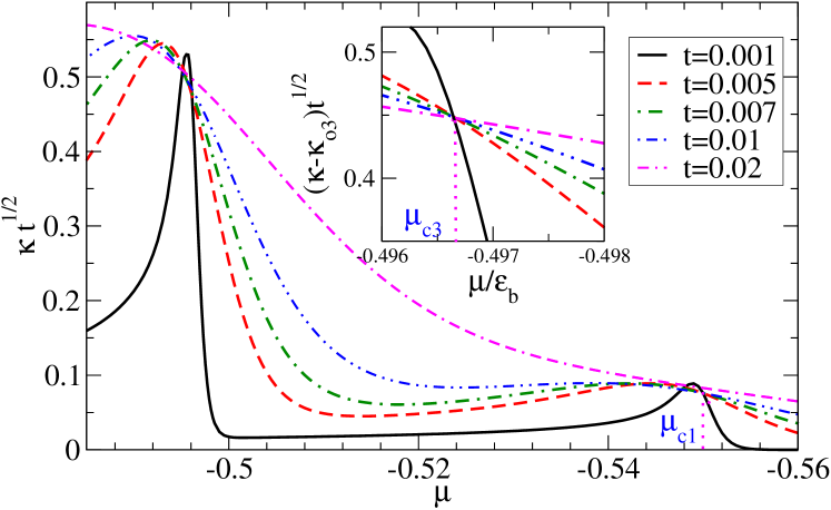
Figure 7: (Color online) Compressibility $\sqrt{t}\kappa$ (dimensionless) vs $\mu$ for $h=1.1$ at different values of $t$. At the critical point $\mu_{c3}$, there is a background compressibility. The curves truly intersect at a single point after the background is removed.

Acknowledgment. This work is supported by NSF Grant DMR-0907366 and by DARPA under the Army Research Office Grant Nos. W911NF-07-1-0464, W911NF0710576. XWG has been supported by the Australian Research Council. He acknowledges the Ohio State University for their kind hospitality.

Appendix: Coefficients

The pressures (12) and (13) provide the precise equation of states for studying two-component Fermi gases with population imbalance. By iteration we found the analytical equation of state (17) which provides high insights into many-body effect in the so called FFLO phase. The first two coefficients are given in (18). The higher order correction terms are given by

$$Y_{\frac{3}{2}}^{b}=\frac{1}{\pi^{\frac{3}{2}}}\left[f_{-\frac{3}{2}}^{b}\left(\frac{\sqrt{2}}{8}\left(f_{\frac{3}{2}}^{b}\right)^{2}f_{\frac{3}{2}}^{u}+\frac{1}{2}\left(f_{\frac{3}{2}}^{u}\right)^{2}f_{\frac{3}{2}}^{b}+\frac{1}{48}\left(f_{\frac{3}{2}}^{b}\right)^{3}\right.\right.$$

$$\left.\left.+\frac{\sqrt{2}}{3}\left(f_{\frac{3}{2}}^{u}\right)^{3}\right)+f_{-\frac{1}{2}}^{b}\left(\frac{3}{16}\left(f_{\frac{3}{2}}^{b}\right)^{2}f_{\frac{1}{2}}^{b}+\frac{1}{\sqrt{2}}\left(f_{\frac{3}{2}}^{b}\right)^{2}f_{\frac{1}{2}}^{u}\right.\right.$$

$$\left.\left.+\frac{3}{2}\left(f_{\frac{3}{2}}^{u}\right)^{2}f_{\frac{1}{2}}^{b}+2f_{\frac{3}{2}}^{b}f_{\frac{3}{2}}^{u}f_{\frac{1}{2}}^{u}+\frac{3\sqrt{2}}{4}f_{\frac{3}{2}}^{b}f_{\frac{3}{2}}^{u}f_{\frac{1}{2}}^{b}\right)\right.$$

$$\left.+f_{\frac{1}{2}}^{b}\left(\frac{1}{\sqrt{2}}\left(f_{\frac{1}{2}}^{b}\right)^{2}f_{\frac{3}{2}}^{u}+\frac{1}{8}\left(f_{\frac{1}{2}}^{b}\right)^{2}f_{\frac{3}{2}}^{b}+\frac{1}{\sqrt{2}}\left(f_{\frac{3}{2}}^{b}\right)^{2}f_{-\frac{1}{2}}^{u}\right.\right.$$

$$\left.\left.+2f_{\frac{1}{2}}^{b}f_{\frac{1}{2}}^{u}f_{\frac{3}{2}}^{u}+\sqrt{2}f_{\frac{1}{2}}^{b}f_{\frac{1}{2}}^{u}f_{\frac{3}{2}}^{b}\right)\right]$$

$$-\frac{1}{\sqrt{\pi}}\left(\sqrt{2}f_{\frac{1}{2}}^{b}f_{\frac{5}{2}}^{u}+\frac{1}{16}\left(f_{\frac{3}{2}}^{b}\right)^{2}+\frac{1}{\sqrt{2}}f_{\frac{3}{2}}^{b}f_{\frac{3}{2}}^{u}\right),$$

$$Y_{\frac{3}{2}}^{u}=\frac{1}{\pi^{\frac{3}{2}}}\left[\frac{1}{6}\left(f_{\frac{3}{2}}^{b}\right)^{3}f_{-\frac{3}{2}}^{u}+f_{-\frac{1}{2}}^{b}\left(\frac{1}{8}\left(f_{\frac{3}{2}}^{b}\right)^{2}f_{-\frac{1}{2}}^{u}\right.\right.$$

$$\left.\left.+\left(f_{\frac{3}{2}}^{b}\right)^{2}f_{\frac{1}{2}}^{u}+\frac{1}{\sqrt{2}}f_{\frac{3}{2}}^{u}f_{\frac{3}{2}}^{b}f_{\frac{1}{2}}^{u}\right)\right.$$

$$\left.+f_{\frac{1}{2}}^{b}\left(\frac{1}{2}\left(f_{\frac{3}{2}}^{b}\right)^{2}f_{-\frac{1}{2}}^{u}+\sqrt{2}\left(f_{\frac{1}{2}}^{u}\right)^{2}f_{\frac{3}{2}}^{b}+\frac{1}{\sqrt{2}}f_{\frac{1}{2}}^{b}f_{\frac{1}{2}}^{u}f_{\frac{3}{2}}^{u}\right.\right.$$

$$\left.\left.+\frac{1}{4}f_{\frac{1}{2}}^{b}f_{\frac{1}{2}}^{u}f_{\frac{3}{2}}^{b}+\sqrt{2}f_{\frac{3}{2}}^{b}f_{\frac{3}{2}}^{u}f_{-\frac{1}{2}}^{u}\right)\right]$$

$$-\frac{1}{\sqrt{\pi}}\left(\frac{1}{2}f_{\frac{1}{2}}^{u}f_{\frac{5}{2}}^{b}+f_{\frac{3}{2}}^{b}f_{\frac{3}{2}}^{u}\right),$$

which reveal cluster-cluster interacting effect.

References

• (1) C. N. Yang, Phys. Rev. Lett. 19, 1312 (1967); M. Gaudin, Phys. Lett. A 24, 55 (1967)
• (2) M. Takahashi, Thermodynamics of One-Dimensional Solvable Models, Cambridge University Press, Cambridge, (1999)
• (3) F.H.L. Essler, et.al. The One-Dimensional Hubbard Model (Cambridge University Press, Cambridge, 2005).
• (4) T. Giamarchi, Quantum Physics in one dimension, Oxford University Press, Oxford (2004)
• (5) G. Orso, Phys. Rev. Lett. 98, 070402 (2007)
• (6) H. Hu, X.-J. Liu and P. Drummond, Phys. Rev. Lett. 98, 070403 (2007)
• (7) X.-W. Guan, M. T. Batchelor, C. Lee and M. Bortz, Phys. Rev. B 76, 085120 (2007).
• (8) T. Iida and M. Wadati, J. Phys. Soc. Jpn, 77, 024006 (2008)
• (9) A. E. Feiguin and F. Heidrich-Meisner, Phys. Rev. B 76 220508 (2008)
• (10) M. Casula, D M. Ceperley and E. J. Mueller, Phys. Rev. A 78, 033607 (2008).
• (11) P. Kakashvili and C. J. Bolech, Phys. Rev. A, 79, 041603(R) (2009).
• (12) P. Fulde and R. A. Ferrell, Phys. Rev. 135, A550 (1964); A. I. Larkin and Yu. N. Ovchinnikov, Sov. Phys. JETP 20, 762 (1965).
• (13) Liao Y, et. al, Nature 467, 567 (2010)
• (14) Qi Zhou and Tin-Lun Ho, Phys. Rev. Lett. 105, 245702 (2010)
• (15) E. Zhao, X.-W. Guan, W. V. Liu, M. T. Batchelor and M. Oshikawa, Phys. Rev. Lett. 103, 140404 (2009)
• (16) C. N. Yang, Selected papers 1945-1980, W. H. Freeman and Company (1983).
• (17) C. N. Yang and C. P. Yang, J. Math. Phys. 10, 1115 (1969).
• (18) Our approach is different from that of Ref. Orso . The equation (8) in Ref. Orso can be expressed as $\mu=-\frac{1}{2}-\frac{1}{2\pi}\left[2Q-\left(2\mu+2h+1)\tan^{-1}(2Q)\right)\right]$ with $Q=\sqrt{(\mu+h)/2}$ in dimensionless unit, which is the same as our result (3) via a rescaling $h\to h/2$.
• (19) The equations in Ref.Erhai is obtained by (i) approximating the $[...]$ in Eq.(12) and (13) by 1, (ii) omitting the $t^{3/2}$ correction terms in Eq.(15), and (iii) by taking the $Tc\rightarrow\infty$ in string equations Takahashi .
• (20) The figure was prepared by X.-G. Yin. The analytical result of quantum criticality obtained in this paper(arXiv: 1010.130) has inspired further study of quantum critical phenomena of the Fermi gas in an harmonic trap, see X.-G. Yin, X.-W. Guan, S. Chen and M. T. Bachelor, Phys. Rev. A 84, 011602(R) (2011).
• (21) M. P. A. Fisher, P. B. Weichman, G. Grinstein and D. F. Fisher, Phys. Rev. B 40, 546 (1989).
• (22) S. Sachdev, Quantum Phase transitions (Cambridge University Press, Cambridge, England, 1999).
• (23) K. R. A. Hazzard and E. J. Mueller, Phys. Rev. A 84, 013604 (2011).
• (24) E. Mueller, private communication.