Identification of strong photometric activity in the components of LHS 1070

Abstract

Context. Activity in low-mass stars is an important ingredient in the evolution of such objects. Fundamental physical properties such as age, rotation, magnetic field are correlated with activity.

Aims. We show that two components of the low-mass triple system LHS 1070 exhibit strong flaring activity. We identify the flaring components and obtained an improved astrometric solution for the LHS 1070 $\mathcal{A}$/($\mathcal{B}$+$\mathcal{C}$) system.

Methods. Time-series CCD observations were used to monitor LHS 1070 in the B and I_C bands. H-band data were used to obtain accurate astrometry for the LHS 1070 $\mathcal{A}$/($\mathcal{B}$+$\mathcal{C}$) system.

Results. We have found that two components of the triple system LHS 1070 exhibit photometric activity. We identified that components $\mathcal{A}$ and $\mathcal{B}$ are the flaring objects. We estimate the total energy, $\sim 2.0\times 10^{33}$ ergs, and the magnetic field strength, $\sim$ 5.5 kG, of the flare observed in LHS 1070 $\mathcal{B}$. This event is the largest amplitude, $\Delta\rm B\gtrsim 8.2$ mag, ever observed in a flare star.

Conclusions.

1 Introduction

LHS 1070 is a triple system of low-mass stars at a distance of $7.72\pm 0.15\,{\rm pc}$ (Costa et al. 2005). Component $\mathcal{A}$ has spectral type M5.5-6 and components $\mathcal{B}$ and $\mathcal{C}$ have spectral types M8.5 and M9-9.5, respectively (Leinert et al. 2000). There is a great deal of interest in this system since the astrometric orbits (specially of components $\mathcal{B}$+$\mathcal{C}$) are well determined, making possible the derivation of precise masses. Seifahrt et al. (2008) obtained values of $0.157\pm 0.009\,{\rm M}_{\odot}$ for the combined dynamical mass of the $\mathcal{B}$+$\mathcal{C}$ components and $0.272\pm 0.017\,{\rm M}_{\odot}$ for the combined dynamical mass of the whole system. The masses are close to the H-burning limit making these objects interesting targets for detailed studies of the transition between low-mass stars and brown dwarfs.

Besides the low masses, the stars in LHS 1070 present other interesting features: the rotational velocities are $v\sin i\simeq 8,16,16\,{\rm km\,s}^{-1}$ for components $\mathcal{A}$, $\mathcal{B}$ and $\mathcal{C}$, respectively. While components $\mathcal{A}$ and $\mathcal{B}$ present signs of activity with H$\alpha$ emission, component $\mathcal{C}$ does not (Reiners et al. 2007). LHS 1070 also shows intense radio emission (Berger 2006). Under the reasonable assumptions of coevality and spin alignment, Reiners et al. (2007) use a Skumanich-like law (Skumanich 1972) with a variable breaking-law index to estimate an age of $\sim 1\,{\rm Gyr}$ for the system.

In this work we report on photometric evidences for strong activity in the $\mathcal{A}$ and $\mathcal{B}$ components of LHS 1070 and discuss the importance of these results in the context of low-mass stars.

2 Observations

The data were collected along an observational program on activity of low-mass stars that is being carried out with the facilities of Laboratório Nacional de Astrofísica (LNA/MCT), in Brazil. We have selected 30 objects in the Southern Hemisphere for at least three differential photometry observing sessions. They were chosen according criteria of being low-mass objects, having suitable comparison stars in a small field-of-view, and being bright enough to be observed even at the 0.6-m telescopes. Table 1 summarizes the characteristics of the data collected for LHS 1070. $N$ is the number of individual images obtained with integration time t_exp. The H-band images were obtained mainly to improve the astrometric solution for the orbital elements of the pair $\mathcal{A}$/($\mathcal{B}$+$\mathcal{C}$).

Table 1: Log of the photometric observations

Date	$N$	texp(s)	Telescope	Filter
Jul 04, 2008	140	30	1.6-m	B
Jul 05, 2008	150	30	1.6-m	B
Aug 25, 2008	653	20	0.6-m	IC
Aug 26, 2008	640	20	0.6-m	IC
Aug 27, 2008	600	20	0.6-m	IC
Aug 28, 2008	570	20	0.6-m	IC
Oct 10, 2008	100	1	1.6-m	H
Sep 01, 2009	100	1	1.6-m	H

3 Data reduction

The reduction of the data was done with the usual IRAF  cl  tasks and consists of subtracting a master median bias image from each program image, and dividing the result by a normalized flat-field. In the H-band, additional steps of linearization and sky subtraction from dithered images were used in the preparation of the data. We treated the photometry extraction in the B- and I_C/H-bands in slightly different ways. The reason for this will become clear in the following discussion.

In the B-band, component $\mathcal{A}$ dominates the flux of the system. This allows us to extract the relevant fluxes using plain aperture photometry. In the flare event (see Figure 1), since additional light could be coming from components $\mathcal{B}$ or $\mathcal{C}$, we fitted a double 2-D Moffat function to the stellar profile.

In the I_C-band, since in principle both $\mathcal{B}$ and $\mathcal{C}$ components could contribute with substantial flux, we fitted simultaneously three 2-D Moffat functions to the stellar profile leaving only the position of component $\mathcal{A}$ and the amplitudes of the three components as free parameters to be searched for. Essentially the same procedure is used for the H-band data. The distances $\mathcal{A}$-$\mathcal{B}$ and $\mathcal{A}$-$\mathcal{C}$ were obtained from the orbital elements listed in Table 3 for LHS 1070 $\mathcal{A}$/($\mathcal{B}$+$\mathcal{C})$ and the orbital elements for LHS 1070 $\mathcal{B}$/$\mathcal{C}$ from Seifahrt et al. (2008). Our own measurements were used to improve the astrometric solution for the pair $\mathcal{A}$/($\mathcal{B}$+$\mathcal{C})$ (see Section 4.2). In all cases we used the amoeba routine of Press et al. (1992) for the fitting procedure.

In order to increase the stability of the fits, for both bands we fixed the Moffat parameters derived from the profile of star 6417-00147-1 in the Tycho catalog and used $\beta=4.765$ as in Trujillo et al. (2001). This star is located at $\Delta\alpha=103.13\,{\rm arcsec}$ and $\Delta\delta=157.32\,\rm{arcsec}$ from LHS 1070 $\mathcal{A}$.

Figure 1 shows the B-band differential photometry for LHS 1070 on July 4, 2008. As one can see, a very strong flare characterized by an e-folding decay time of $\sim 165\,{\rm sec}$ and a factor of $\sim 80$ increase in brightness with respect to quiescence was observed. Figure 2 shows the I_C-band light curve of an event with a longer time-scale (the e-folding time is $\>\sim 1080\,{\rm sec}$) in August 28th. Unfortunately, the onset of this flare was not observed.

Figure 1: B-band differential photometry of LHS 1070 on July 04, 2008. The light curves of LHS 1070 and of a comparison star are presented with full circles and stars, respectively.

Figure 2: I_C-band differential photometry of LHS 1070 on August 28, 2008. From top to bottom we show the aperture photometry for LHS 1070, the results of the 2-D Moffat function fitting for LHS 1070 $\mathcal{A}$ and LHS 1070 $\mathcal{B}$+$\mathcal{C}$ and the aperture photometry for a faint comparison star in the field.

4 Analysis and results

4.1 Astrometry

Visual examination of the CCD images during the B-band flare suggests a significant displacement of the photocenter of LHS 1070 during the event. 101 pre-flare images allow the average relative position of LHS 1070 $\mathcal{A}$ with respect to a reference star to be measured with $\sim 20$ mas accuracy. As the flare progresses, the photocenter shifts toward North and East indicating that component $\mathcal{A}$ was not the flaring object. Figure 3 shows the differential positions of LHS 1070 with respect to a reference object. To identify which component, $\mathcal{B}$ or $\mathcal{C}$, was responsible for the event, we proceeded as follows. First, we obtained an astrometric solution for the whole field using the registered pre-flare images. Seven stars (excluding LHS 1070) can be used for the astrometry. We used the IRAF ccmap  task to obtain the plate scale (0.315 arcsec/pixel) and rotation of the images ($+0\aas@@fstack{\circ}1$ with respect to North). The position corresponding to the flare was found by fitting a double 2-D Moffat function to the stellar profile in the six images closer to the flare peak. The flare position is shown together with the orbital solutions for LHS 1070 $\mathcal{B}$/$\mathcal{C}$ (Seifahrt et al. 2008) and LHS 1070 $\mathcal{A}$/($\mathcal{B}$+$\mathcal{C}$) (Table 3) in Figure 4. We conclude that the flaring object was component $\mathcal{B}$.

Figure 3: The position of the photocenter of LHS 1070 with respect to a Tycho catalog star. The pre-flare position was obtained using the 101 images before the flare. Its uncertainty can be estimated from the bidimensional distribution of individual positions, and results in a positional accuracy of $\sim 20\,{\rm mas}$. The six images around the peak of the event define the position of the photocenter during the flare. The predicted positions of $\mathcal{B}$ and $\mathcal{C}$ components are marked with a “$\times$” symbol considering component $\mathcal{A}$ at the origin. The box shown in the upper right corner represents the size of one pixel.

Figure 4: Configuration of LHS 1070 on Jul 04, 2008. The solid line represents the trajectory of the barycenter of LHS 1070 $\mathcal{B}$+$\mathcal{C}$ around LHS 1070 $\mathcal{A}$ which is at the origin. The dotted lines show the trajectories of components $\mathcal{B}$ and $\mathcal{C}$ around the barycenter of LHS 1070 $\mathcal{B}$+$\mathcal{C}$, assuming the two components have the same mass. The positions measured by Leinert et al. (2001) and Seifahrt et al. (2008) are shown as open and full squares. Our measurements appear as open circles. The full circle shows our estimated position for the flaring object. The predicted positions of the barycenter of LHS 1070 $\mathcal{B}$+$\mathcal{C}$ and of components $\mathcal{B}$ and $\mathcal{C}$ are marked with a “$\times$” symbol. The box shown in the upper right corner represents the size of one pixel of our detector

.

4.2 Astrometric solution and orbital fitting for LHS 1070 $\mathcal{A}$/($\mathcal{B}$+$\mathcal{C})$

We used the Monte Carlo Markov Chain approach to explore the distribution of probability of the orbital elements of LHS 1070 $\mathcal{A}$/($\mathcal{B}$+$\mathcal{C}$). The data from Seifahrt et al. (2008), Leinert et al. (2001) and our own measurements (see Table 2) were used in this analysis. The orbital elements distributions of Seifahrt et al. (2008) were used as prior information to obtain the posterior distribution of the parameters. Figure 5 shows the marginal distributions and Table 3 presents the numerical values with the associated $\pm 68\%$ uncertainties.

It is interesting to compare the results of the orbital elements obtained for the LHS 1070 $\mathcal{A}$/($\mathcal{B}$+$\mathcal{C}$) system with the results obtained by Seifahrt et al. (2008) for LHS 1070 $\mathcal{B}$/$\mathcal{C}$. The orbits of the three components are, within the uncertainties, coplanar.

Table 2: Distances between the photocenters of LHS 1070 $\mathcal{B}$+$\mathcal{C}$ and LHS 1070 $\mathcal{A}$.

Date	$\Delta\alpha$ (′′)	$\Delta\delta$ (′′)
Oct 10, 2008	0.644$\pm$0.022	1.344$\pm$0.022
Sep 01, 2009	0.665$\pm$0.013	1.303$\pm$0.013

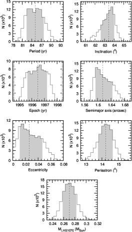
Figure 5: Marginal distribution of posterior probability for the orbital elements of LHS 1070 $\mathcal{A}$/($\mathcal{B}$+$\mathcal{C}$). The dashed line shows the median and the grey areas mark the $\pm 68\%$ confidence regions.

Table 3: Orbital elements for the LHS 1070 $\mathcal{A}$/($\mathcal{B}$+$\mathcal{C}$) binary.

Parameter	Value
P (yr)	85.1$\pm 2.7$
$T_{0}$ (yr)	1996.48${}^{+0.72}_{-0.82}$
$a$ (′′)	1.615${}^{+0.029}_{-0.021}$
$e$	0.026${}^{+0.021}_{-0.015}$
$i$ (∘)	63.44${}^{+0.57}_{-0.83}$
$\Omega$ (∘)	14.24${}^{+0.42}_{-0.47}$
M${}_{\textrm{\tiny{LHS\,1070}}}\leavevmode\nobreak\$(M⊙)	0.270$\pm 0.012$

4.3 The flare in LHS 1070 $\mathcal{B}$

As one can see in Figure 1, the B-band flare is relatively fast, with a rise-time of $\sim$225$\,{\rm s}$. The decay back to quiescence took $\sim$880$\,{\rm s}$. The duration of the event is thus $\sim$1100$\,{\rm s}$. The flare amplitude with respect to the quiescent magnitude of component $\mathcal{A}$ is $\sim$4.8 mag. However, since component $\mathcal{B}$ is the flaring object, and adopting B $=17.17$ and B $=20.57$ (Leinert et al. 2000) as the quiescent B-magnitudes of components $\mathcal{A}$ and $\mathcal{B}$, we obtain $\sim$8.2 mag as a lower limit for the flare amplitude.

4.3.1 Luminosity and total energy

The luminosity of the flare can be estimated as follows. The monochromatic flux associated to the apparent quiescent magnitude B is,

$$F_{\rm{\tiny{B}},\lambda}=F_{\tiny{\rm B}_{0}}10^{-\left(\frac{\tiny{\rm B}}{2.5}\right)},$$ (1)

where $F_{\tiny{\rm B}_{0}}=6.32\times 10^{-9}\,\rm erg\,\rm cm^{-2}\,\rm s^{-1}$ $\mathring{\rm A}^{-1}$ is the absolute flux corresponding to zero magnitude (Bessell et al. 1998). The quiescent level observed prior to the flare is due to component $\mathcal{A}$. It corresponds to B=17.17 (Leinert et al. 2000). This sets a reference level to which the flare flux may be referred to. Thus, the quiescent level of component $\mathcal{A}$, expressed as luminosity in the B-band is,

$$L_{\tiny{\rm B}}=4\pi D^{2}F_{\tiny{\rm B}_{0}}\Delta\lambda 10^{-\left(\frac{\tiny{\rm B}}{2.5}\right)}\sim 5.4\times 10^{27}\rm{erg}\,\rm{s}^{-1},$$ (2)

where $\Delta\lambda=890\,\mathring{\rm A}$ is the B-band FWHM (Bessell 2005) and $D=7.72\,\rm pc$ is the distance to the system. The luminosity of the event can be obtained using Eq. 2 and the differential magnitudes of each point along the flare with respect to the quiescent level. The time-integral under the flare luminosity light curve is the total energy of the flare in the B-band. From this procedure we obtain $E_{\rm\tiny B}\sim 9.8\times 10^{31}$ erg.

4.3.2 Magnetic field strength

In order to obtain the magnetic field strength, we have to estimate the bolometric energy of the event, $E_{bol}$. We start with the flare energy in the B-band, $E_{\rm\tiny{B}}$, and use the relation among optical, UV and X-ray energies obtained from multispectral observations of flares in low-mass stars (Gershberg 2005),

$$E_{bol}\sim 20.9\,E_{\tiny{\rm B}}\sim 2.0\times 10^{33}\,\rm ergs.$$ (3)

Knowing the total energy irradiated and assuming that this flare has the same mechanisms as in solar flares, we can estimate a lower limit for the magnetic field strength in the region of the event. Stellar flares are caused by sudden changes of magnetic field strength in the stellar corona as result of the reconnection of magnetic field lines (see e.g., Kopp & Pneuman 1976; Priest 1986). Such changes convert magnetic potential energy into plasma acceleration (see e.g., Kuperus 1976; Dauphin 2007). Part of the plasma is released from the star as coronal mass ejection and part is accelerated towards the chromosphere. The latter part interacts with denser plasma converting kinetic energy into thermal energy and is associated with optical and X-ray emission. According to Hawley & Fisher (1992), a blackbody at a temperature $\sim$ 10${}^{4}\,\rm K$ can be used as a raw description of the optical emitting region. In terms of fractional area $X$ on the star (Hawley et al. 2003), we have the flux at the maximum of the flare given by

$$F_{\lambda}=X\frac{R^{2}_{\ast}}{D^{2}}\pi B_{\lambda}(T),$$ (4)

where $T$ is the blackbody temperature, $B_{\lambda}$ is the Planck function, $R_{\ast}$ is the radius of the star and $D$ is the distance to the object. Using Eq. 1 and $\Delta\rm B\sim 4.8$ for the maximum flare amplitude, the flux at the B-band pivotal wavelength is $F_{\rm B}\sim 7.12\times 10^{-14}\,\rm erg\,cm^{-2}\,s^{-1}\,\mathring{\rm A}^{-1}$. With the aid of the mass-radius relation for low-mass stars Chabrier et al. (2009), and $M=0.0815\,\rm M_{\odot}$ for LHS 1070 $\mathcal{B}$ (Leinert et al. 2000), the fractional area obtained is $\sim 1.4\times 10^{-2}$. The corresponding covered area and spherical volume are $\sim 1.4\times 10^{18}\rm\,cm^{2}$ and $\sim$1.7$\times 10^{27}\leavevmode\nobreak\ {\rm cm}^{3}$, respectively.

Using the simplest case where the volume occupied by the magnetic field lines is spherical, and assuming the dimension of the acceleration region equal to the emitting region (Aschwanden 2002) and considering the standard model, i.e., the total flare energy being produced by magnetic energy decay (see e.g., Brown et al. 1994; Dauphin 2007), we can estimate the magnetic field strength, $B$, using the relation:

$$\frac{E_{bol}}{V}=\frac{B^{2}}{8\pi}.$$ (5)

This gives a value of $B\sim 5.5$ kG in the flaring region. Notice that this is a lower limit. Reiners et al. (2007) obtained an average $B$-field of $\sim 4$ kG over the entire star, from analysis of spectroscopic data. We would expect to have larger values of the magnetic field strength in a flare.

5 Discussion

As one can see in Figure 2, component $\mathcal{A}$ was responsible for the flare on August 28, 2008. The photometric activity detected in both $\mathcal{A}$ and $\mathcal{B}$ components is consistent with the spectroscopic results of Leinert et al. (2000).

Photometric activity was unknown in LHS 1070 before. The noticeable flare in LHS 1070 $\mathcal{B}$ shows that even close to the Hydrogen-burning limit, relatively old objects can still show significant magnetic fields. The activity level observed in the components of the LHS 1070 system, and the age estimated by Reiners et al. (2007) are in agreement with the activity lifetime-spectral type relation discussed by West et al. (2008).

In order to stress the importance of the event observed in LHS 1070 $\mathcal{B}$, we recollect the most impulsive optical flares previously recorded on dMe stars. Impulsive stellar flares are events lasting $\sim$100-1000 s with large amplitudes. Gershberg (2005) describes several flares among which the most impulsive was the one observed by de de Jager et al. (1989) on a dM5.5e star, UV Cet, on December 23, 1985, with amplitude of 5 mag in the B-band. Another impulsive flare with 7 mag amplitude at blue wavelengths was observed by Bond (1976) on a dMe star. Stelzer et al. (2006) reported a multi-wavelength observation of a flare on LP 412-31. This object has spectral type M8 and showed a 6 mag amplitude flare in the V-band. More recently, Kowalski et al. (2010) observed a flare on the dM4.5e star YZ CMi with amplitude $\sim 6$ mag in the U-band. Thus, since the lower limit for the LHS 1070 $\mathcal{B}$ flare presented here is $\sim$8.2 mag in the B-band, we conclude that this event has the largest amplitude ever observed in a flare star.

Regarding the energy released in flares, Gershberg (2005) discusses a few events observed in BY Dra and AD Leo in the B-band that reached $\sim 10^{35}$ erg. However, the time-scales for these events are larger than the observed by us. Besides, those objects have spectral types earlier than that of LHS 1070 $\mathcal{B}$. This means that a fair comparison between the energy released in the event observed on LHS 1070 $\mathcal{B}$ and other objects should be restricted to similar spectral types and similar time-scales. Using these criteria there is only one object that has a similar energy budget in a flare: the M8 dwarf, LP 412-31 for which $E_{bol}\sim 6\times 10^{32}$ erg.