UFSCARF-TH-10-10

The Yang-Baxter Equation for $\mathcal{PT}$ Invariant Nineteen Vertex Models
R.A. Pimenta and M.J. Martins

Universidade Federal de São Carlos
Departamento de Física
C.P. 676, 13565-905  São Carlos(SP), Brazil

We study the solutions of the Yang-Baxter equation associated to nineteen vertex models invariant by the parity-time symmetry from the perspective of algebraic geometry. We determine the form of the algebraic curves constraining the respective Boltzmann weights and found that they possess a universal structure. This allows us to classify the integrable manifolds in four different families reproducing three known models besides uncovering a novel nineteen vertex model in a unified way. The introduction of the spectral parameter on the weights is made via the parameterization of the fundamental algebraic curve which is a conic. The diagonalization of the transfer matrix of the new vertex model and its thermodynamic limit properties are discussed. We point out a connection between the form of the main curve and the nature of the excitations of the corresponding spin-1 chains.

PACS numbers: 05.50+q, 02.30.IK

Keywords: Yang-Baxter Equation, Lattice Integrable Models, Bethe Ansatz

October 2010

1 Introduction

An important concept in the theory of soluble two-dimensional lattice models of statistical mechanics is to embed the respective transfer matrices into a family of pairwise commuting operators [1]. Let $T_{L}\left(\omega_{1}^{(i)},\ldots,\omega_{n}^{(i)}\right)$ denote the transfer matrix on a chain of size $L$ with Boltzmann weights $\omega_{1}^{i},\ldots,\omega_{n}^{(i)}$. This approach requires that the transfer matrix fulfill the following property,

$$\left[T_{L}\left(\omega_{1}^{(1)},\ldots,\omega_{n}^{(1)}\right),T_{L}\left(\omega_{1}^{(2)},\ldots,\omega_{n}^{(2)}\right)\right]=0,$$ (1)

for arbitrary $L$ and weights $\omega_{1}^{(i)},\ldots,\omega_{n}^{(i)}$ for $i=1,2$.

At first sight it appears one needs to verify an infinite number of constraints for the weights since Eq.(1) should be valid for any values of $L$. This is however not the case since Baxter argued that a finite number of local conditions on the weights are sufficient to assure the commutativity among distinct transfer matrices for arbitrary $L$ [2]. These conditions can be written as a matrix equation whose structure depend much on the family of lattice model under consideration. In what follows we shall discuss them for a relevant class of lattice systems denominated vertex models.

Lets us for example consider a vertex model on a square lattice of size $L\times L$. The respective statistical configurations sit on the edges of the lattice. In the simplest case the number of states living on the horizontal and vertical edges are the same and take values on a set of integers numbers $1,2,\ldots,N$. Furthermore, to each vertex configuration $a,b,c,d=1,\ldots,N$ is assigned the Boltzmann weight $\mathcal{L}\left(a,c|b,d\right)$ as defined in Figure 1.

Figure 1: Elementary configuration in a vertex model on a square lattice.

The sufficient condition for the commutativity of two distinct transfer matrices associated to a given vertex model for arbitrary $L$ is the celebrated Yang-Baxter equation [2]. Considering the notation of Figure 1, these set of functional relations can be written as follows,

$$\sum_{\gamma_{1},\gamma_{2},\gamma_{3}=1}^{N}R\left(a_{1},\gamma_{1}|a_{2},\gamma_{2}\right)\mathcal{L}^{(1)}\left(\gamma_{1},b_{1}|a_{3},\gamma_{3}\right)\mathcal{L}^{(2)}\left(\gamma_{2},b_{2}|\gamma_{3},b_{3}\right)=$$

$$\sum_{\gamma_{1},\gamma_{2},\gamma_{3}=1}^{N}\mathcal{L}^{(2)}\left(a_{2},\gamma_{2}|a_{3},\gamma_{3}\right)\mathcal{L}^{(1)}\left(a_{1},\gamma_{1}|\gamma_{3},b_{3}\right)R\left(\gamma_{1},b_{1}|\gamma_{2},b_{2}\right).$$ (2)

where $R(a,c|b,d)$ are the elements of an invertible $N^{2}\times N^{2}$ matrix often called $R-$matrix.

In order to classify solvable vertex models with given statistical configurations one has to find the possible solutions of the corresponding Yang-Baxter equation. In principle, we can consider this problem by following the method devised by Baxter for two states vertex models [2]. We start by eliminating the matrix elements $R(a,b|c,d)$ with the help of suitable subset of relations derived from Eq.(2). The remaining functional equations will then depend only on the weights $\mathcal{L}^{(1)}(a,b|c,d)$ and $\mathcal{L}^{(2)}(a,b|c,d)$ which need to be decoupled by means of the technique of separation of variables. This step is essential to reveal us the algebraic invariants constraining the Boltzmann weights parameter space. The parameterization of such manifolds provides us the dependence of Boltzmann weights on spectral parameters which is for instance useful to formulate the algebraic Bethe ansatz [3, 4, 5].

The implementation of all the steps described above, even for a given fixed vertex state configuration, is in general a tantalizing problem in mathematical physics. The concrete results are mostly concentrated on vertex models having two states per edge, see for instance [6, 7, 8]. In this case the non-trivial models that have been uncovered are mainly associated to the algebraic manifolds of the asymmetric six vertex model [9], the symmetric eight vertex model [10] and the so-called free-fermions systems [11]. The difficulties of the problem increase with the number $N$ of states due to the proliferation of the possible allowed weights that are ultimately fixed by different classes of functional relations. The merit of this approach is that it makes possible an unambiguous classification of integrable vertex models with a given statistical configuration from first principles.

The purpose of this paper is to begin a study of the Baxter method for three state models satisfying the so-called ice-rule. The respective statistical configuration leads us to the total number of nineteen Boltzmann weights. Here we shall consider a relevant subclass of such models whose weights are invariant by the joint action of the parity and time ($\mathcal{PT}$) reversal symmetry. For this family of nineteen vertex models we show that the dependence of the underlying algebraic curves on the respective weights are rather universal. The possible solvable vertex models are classified by the distinct branches of certain invariants values entering the definition of these manifolds. This general analysis provides us the classification of nineteen vertex models in four different families. The first three of them have already been discovered in the context of integrable spin-1 XXZ chain [12], the quantum inverse scattering of the Mikhailov-Shabat model [13] and the quantum algebra $U_{q}[SU(2)]$ at roots of unity [14, 15, 16]. Interesting enough, our results reveal that these models have the same underlying algebraic background despite their rather distinct quantum group origin. To the best of our knowledge the fourth uncovered vertex model is new in the literature.

We have organized this paper as follows. For sake of completeness we review in next section the main characteristics of the nineteen vertex models. In section 3 we consider the analysis of the functional relations coming from the Yang-Baxter equation. We develop a systematic way to solve such Yang-Baxter relations leading us to determine the algebraic curves fulfilled by the Boltzmann weights. It turns out that the principal algebraic curve is a conic involving three basic independent weights. The remaining amplitudes of the parameter space are remarkably resolved in terms of ratios of polynomials depending on such basic weights. This makes it possible to classify the $\mathcal{PT}$ invariant nineteen vertex models from a unified perspective. In section 4 we discuss the parameterization of the Boltzmann weights in terms of a spectral parameter and the associated spin-1 Hamiltonians. We note that the geometric form of the fundamental algebraic curve is directly related to the nature of the excitations of the corresponding spin chains. In section 5 we present the eigenvalues of the transfer matrix associated to the new nineteen vertex model and its respective Bethe ansatz equation. We investigate the bulk properties of this model providing additional support to the mentioned relationship among the curve geometry and the behaviour of the spin-1 chain excitations. Our conclusions are presented in section 6. In the appendices we summarize some technical details useful for the understanding of the main text.

2 The nineteen vertex model

In this section we shall review the main features of the nineteen vertex model. This lattice model has three states per edge which here will be denoted by $a,b,c,d=0,\pm$. The allowed statistical configurations compatible with the ice-rule $a+b=c+d$ lead us to nineteen different Boltzmann weights. These weights are represented in Figure 2 where the respective subscripts emphasizes the non-null charge sectors $a+b$.

Figure 2: The vertex configurations of a general nineteen vertex model on a square lattice.

In this paper we will investigate the integrable manifolds of nineteen vertex models whose weights are $\mathcal{PT}$ invariant. This invariance relates some of the weights leading us to subclass of three-state vertex models with fourteen distinct Boltzmann weights. More precisely, the $\mathcal{PT}$ symmetry imposes the following relationship among the weights of Figure 2,

$$\tilde{b}_{\pm}=b_{\pm},\,\tilde{f}=f,\,e=d,\,\tilde{e}=\tilde{d}.$$ (3)

We begin by introducing a common notation for the Boltzmann weights of such family of nineteen vertex models. Taking into account the parameter subspace (3) one can represent the content of the $\mathcal{L}^{(i)}$-operators by the following matrix,

$$\mathcal{L}^{(i)} = a_{+}^{(i)}e_{1,1}\otimes e_{1,1}+b_{+}^{(i)}\left[e_{1,1}\otimes e_{2,2}+e_{2,2}\otimes e_{1,1}\right]+f^{(i)}\left[e_{1,1}\otimes e_{3,3}+e_{3,3}\otimes e_{1,1}\right]$$ (4)

$$+ b_{-}^{(i)}\left[e_{2,2}\otimes e_{3,3}+e_{3,3}\otimes e_{2,2}\right]+g^{(i)}e_{2,2}\otimes e_{2,2}+a_{-}^{(i)}e_{3,3}\otimes e_{3,3}+h^{(i)}e_{1,3}\otimes e_{3,1}$$

$$+ \tilde{h}^{(i)}e_{3,1}\otimes e_{1,3}+c_{+}^{(i)}e_{1,2}\otimes e_{2,1}+\tilde{c}_{+}^{(i)}e_{2,1}\otimes e_{1,2}+c_{-}^{(i)}e_{2,3}\otimes e_{3,2}+\tilde{c}_{-}^{(i)}e_{3,2}\otimes e_{2,3}$$

$$+ d^{(i)}\left[e_{1,2}\otimes e_{3,2}+e_{2,3}\otimes e_{2,1}\right]+\tilde{d}^{(i)}\left[e_{2,1}\otimes e_{2,3}+e_{3,2}\otimes e_{1,2}\right],~{}~{}\mathrm{for}~{}~{}i=1,2,$$

where $e_{a,b}$ denote $3\times 3$ Weyl matrices.

By substituting the $\mathcal{L}^{(i)}-$operators (4) in the Yang-Baxter equation (2) we are able to determine the null matrix elements of the $R-$matrix. Under the mild assumption that the weight $a_{\pm}^{(i)}$ are in general distinct from $b_{\pm}^{(i)}$ and $f^{(i)}$ it is not difficult to see that the $R-$matrix has the same form of the $\mathcal{L}^{(i)}-$operators. For latter convenience we shall therefore express the $R-$matrix as,

$$R = a_{+}^{(0)}e_{1,1}\otimes e_{1,1}+b_{+}^{(0)}\left[e_{1,1}\otimes e_{2,2}+e_{2,2}\otimes e_{1,1}\right]+f^{(0)}\left[e_{1,1}\otimes e_{3,3}+e_{3,3}\otimes e_{1,1}\right]$$ (5)

$$+ b_{-}^{(0)}\left[e_{2,2}\otimes e_{3,3}+e_{3,3}\otimes e_{2,2}\right]+g^{(0)}e_{2,2}\otimes e_{2,2}+a_{-}^{(0)}e_{3,3}\otimes e_{3,3}+h^{(0)}e_{1,3}\otimes e_{3,1}$$

$$+ \tilde{h}^{(0)}e_{3,1}\otimes e_{1,3}+c_{+}^{(0)}e_{1,2}\otimes e_{2,1}+\tilde{c}_{+}^{(0)}e_{2,1}\otimes e_{1,2}+c_{-}^{(0)}e_{2,3}\otimes e_{3,2}+\tilde{c}_{-}^{(0)}e_{3,2}\otimes e_{2,3}$$

$$+ d^{(0)}\left[e_{1,2}\otimes e_{3,2}+e_{2,3}\otimes e_{2,1}\right]+\tilde{d}^{(0)}\left[e_{2,1}\otimes e_{2,3}+e_{3,2}\otimes e_{1,2}\right].$$

We emphasize here that we are interested to classify genuine nineteen vertex models and therefore all the weights $a_{\pm}^{(i)}$, $b_{\pm}^{(i)}$, $c_{\pm}^{(i)}$, $\tilde{c}_{\pm}^{(i)}$, $d^{(i)}$, $\tilde{d}^{(i)}$, $f^{(i)}$, $g^{(i)}$, $h^{(i)}$ and $\tilde{h}^{(i)}$ for $i=0,1,2$ are assumed to be non-null. We recall that a classification of solvable three-state vertex models has been attempted before in the literature [17]. In the work [17], more stringent symmetry conditions for the weights were assumed besides the fact that some of them could be null. As a result, the only strict nineteen vertex model found was the standard Fateev-Zamolodchikov spin one model [12].

3 The Yang-Baxter Equation

The purpose of this section is to investigate the functional relations for the Boltzmann weights which are derived by substituting the $\mathcal{L}^{(i)}-$operator (4) and the $R$-matrix (5) structures into the Yang-Baxter equation (2). We find that the functional relations can be classified in terms of the number of distinct triple product of weights. It turns out the minimum number of triple products is two while the maximum is five. In Table 1 we summarize the number of different equations having two, three, four and five types of triple product of weights. Clearly, both the number and the structure of the functional relations to be analyzed are far more involving than that associated to the $N=2$ state vertex model satisfying the ice-rule . We shall therefore start our discussion by first solving the simplest relations containing two triple products.

Number of triple products	Number of equations
two	6
three	36
four	57
five	24

Table 1: The dependence of the number of distinct functional relations on the respective number of triple products.

3.1 Two terms relations

The six equations possessing only two different types of triple product of weights are given by,

$$c_{\pm}^{(0)}\tilde{c}^{(1)}_{\pm}c_{\pm}^{(2)}-\tilde{c}_{\pm}^{(0)}c_{\pm}^{(1)}\tilde{c}_{\pm}^{(2)}=0,$$ (6)

$$d^{(0)}\tilde{d}^{(1)}c_{\pm}^{(2)}-\tilde{d}^{(0)}d^{(1)}\tilde{c}_{\pm}^{(2)}=0,$$ (7)

$$c_{\pm}^{(0)}\tilde{d}^{(1)}d^{(2)}-\tilde{c}_{\pm}^{(0)}d^{(1)}\tilde{d}^{(2)}=0.$$ (8)

We first note that the apparent difference between $c^{(i)}_{\pm}$ and $\tilde{c}^{(i)}_{\pm}$ can be gauge away by a transformation preserving the Yang-Baxter equation. Without losing generality we can set,

$$\tilde{c}_{\pm}^{(i)}=c_{\pm}^{(i)},~{}~{}\mathrm{for}~{}~{}i=0,1,2.$$ (9)

By substituting the result (9) in Eqs.(7,8) we conclude that the weight $\tilde{d}^{(i)}$ becomes proportional to $d^{(i)}$,

$$\frac{\tilde{d}^{(i)}}{d^{(i)}}=\Psi,~{}~{}\mathrm{for}~{}~{}i=0,1,2,$$ (10)

where $\Psi$ is our first invariant value.

We shall now turn our attention to the relations involving three types of triple products.

3.2 Three terms relations

By using the solution (9,10) we find that the thirty six relations possessing three triple products are pairwise equivalent leading us to eighteen distinct functional equations. They can be classified in terms of three different groups of six equations given by,

• group $G_{\pm}^{(1)}$

  $$b_{\pm}^{(0)}c_{\pm}^{(1)}c_{\pm}^{(2)}+c_{\pm}^{(0)}a_{\pm}^{(1)}b_{\pm}^{(2)}-c_{\pm}^{(0)}b_{\pm}^{(1)}a_{\pm}^{(2)}=0,$$ (11)

  $$b_{\pm}^{(0)}c_{\pm}^{(1)}b_{\pm}^{(2)}+c_{\pm}^{(0)}a_{\pm}^{(1)}c_{\pm}^{(2)}-a_{\pm}^{(0)}c_{\pm}^{(1)}a_{\pm}^{(2)}=0,$$ (12)

  $$c_{\pm}^{(0)}c_{\pm}^{(1)}b_{\pm}^{(2)}+b_{\pm}^{(0)}a_{\pm}^{(1)}c_{\pm}^{(2)}-a_{\pm}^{(0)}b_{\pm}^{(1)}c_{\pm}^{(2)}=0,$$ (13)

• group $G_{\pm}^{(2)}$

  $$d^{(0)}b_{\pm}^{(1)}b_{\pm}^{(2)}+f^{(0)}d^{(1)}c_{\pm}^{(2)}-d^{(0)}f^{(1)}a_{\pm}^{(2)}=0,$$ (14)

  $$f^{(0)}d^{(1)}b_{\pm}^{(2)}+d^{(0)}b_{\pm}^{(1)}c_{\pm}^{(2)}-b_{\pm}^{(0)}d^{(1)}a_{\pm}^{(2)}=0,$$ (15)

  $$\Psi d^{(0)}d^{(1)}b_{\mp}^{(2)}+f^{(0)}b_{\pm}^{(1)}c_{\mp}^{(2)}-b_{\pm}^{(0)}f^{(1)}c_{\mp}^{(2)}=0,$$ (16)

• group $G_{\pm}^{(3)}$

  $$b_{\pm}^{(0)}b_{\pm}^{(1)}d^{(2)}+c_{\pm}^{(0)}d^{(1)}f^{(2)}-a_{\pm}^{(0)}f^{(1)}d^{(2)}=0,$$ (17)

  $$c_{\pm}^{(0)}b_{\pm}^{(1)}d^{(2)}+b_{\pm}^{(0)}d^{(1)}f^{(2)}-a_{\pm}^{(0)}d^{(1)}b_{\pm}^{(2)}=0,$$ (18)

  $$\Psi b_{\pm}^{(0)}d^{(1)}d^{(2)}+c_{\pm}^{(0)}b_{\mp}^{(1)}f^{(2)}-c_{\pm}^{(0)}f^{(1)}b_{\mp}^{(2)}=0,$$ (19)

where the subscript $\pm$ in Eqs.(11-19) means that each of them splits into two independent functional relations.

Altogether we have eighteen linear homogeneous equations but only eight Boltzmann weights $a_{\pm}^{(0)}$,$b_{\pm}^{(0)}$,$c_{\pm}^{(0)}$, $d^{(0)}$ and $f^{(0)}$ are at our disposal to be eliminated. Therefore, we have a high degree of over-determination to overcome making the solution of Eqs.(11-19) far from being trivial. We shall start our analysis by considering the group $G_{\pm}^{(1)}$ of equations. They are similar to the functional equations underlying the symmetric six-vertex model and can be easily handled. We first eliminate the weights $a_{\pm}^{(0)}$, $b_{\pm}^{(0)}$ in terms of $c_{\pm}^{(0)}$ with the help of Eqs.(11,12). As a result we obtain,

$$\frac{a_{\pm}^{(0)}}{c_{\pm}^{(0)}}=\frac{b_{\pm}^{(1)}a_{\pm}^{(2)}b_{\pm}^{(2)}-a_{\pm}^{(1)}\left\{\left[b_{\pm}^{(2)}\right]^{2}-\left[c_{\pm}^{(2)}\right]^{2}\right\}}{c_{\pm}^{(1)}a_{\pm}^{(2)}c_{\pm}^{(2)}},$$ (20)

$$\frac{b_{\pm}^{(0)}}{c_{\pm}^{(0)}}=\frac{b_{\pm}^{(1)}a_{\pm}^{(2)}-a_{\pm}^{(1)}b_{\pm}^{(2)}}{c_{\pm}^{(1)}c_{\pm}^{(2)}}.$$ (21)

By substituting the above results (20,21) in Eq.(13) we find two separable curves that involve the weights $a_{\pm}^{(i)}$,$b_{\pm}^{(i)}$ and $c_{\pm}^{(i)}$ for $i=1,2$. Their solution leads us to invariants typical of six-vertex models,

$$\frac{\left[a_{\pm}^{(i)}\right]^{2}+\left[b_{\pm}^{(i)}\right]^{2}-\left[c_{\pm}^{(i)}\right]^{2}}{a_{\pm}^{(i)}b_{\pm}^{(i)}}=\Delta_{\pm},~{}~{}\mathrm{for}~{}~{}~{}i=1,2,$$ (22)

where $\Delta_{\pm}$ are free invariant parameters.

We now turn our attention to the relations associated to the group $G_{\pm}^{(2)}$. We start by first eliminating the weights $d^{(0)}$ and $f^{(0)}$ from Eqs.(14,15). Because they can be isolated from equations possessing different charge sectors we need to keep track of their explicit expressions. The compatibility of such distinct solutions will be implemented subsequently. The expressions for $d^{(0)}$ and $f^{(0)}$ are,

$$\frac{d^{(0)}}{c_{\pm}^{(0)}}=\frac{d^{(1)}a_{\pm}^{(2)}}{c_{\pm}^{(1)}}\left\{\frac{b_{\pm}^{(1)}a_{\pm}^{(2)}-a_{\pm}^{(1)}b_{\pm}^{(2)}}{f^{(1)}a_{\pm}^{(2)}b_{\pm}^{(2)}-b_{\pm}^{(1)}\left[b_{\pm}^{(2)}\right]^{2}+b_{\pm}^{(1)}\left[c_{\pm}^{(2)}\right]^{2}}\right\},$$ (23)

$$f^{(0)}=\left[\frac{f^{(1)}a_{\pm}^{(2)}-b_{\pm}^{(1)}b_{\pm}^{(2)}}{d^{(1)}c_{\pm}^{(2)}}\right]d^{(0)},$$ (24)

where as before they are given in terms of the common weights $c_{\pm}^{(0)}$.

We then substitute Eqs.(23,24) in Eq.(16) and by taking into account that the Boltzmann weights are non-null we find the following relation,

$$c_{\mp}^{(2)}\left\{\left(\left[b_{\pm}^{(1)}\right]^{2}+\left[f^{(1)}\right]^{2}\right)a_{\pm}^{(2)}b_{\pm}^{(2)}-b_{\pm}^{(1)}f^{(1)}\left(\left[a_{\pm}^{(2)}\right]^{2}+\left[b_{\pm}^{(2)}\right]^{2}-\left[c_{\pm}^{(2)}\right]^{2}\right)\right\}-\Psi\left[d^{(1)}\right]^{2}a_{\pm}^{(2)}b_{\mp}^{(2)}c_{\pm}^{(2)}=0.$$ (25)

By using the previous invariant (22) on the second term of Eq.(25) one is able to split the weights with index $i=1$ from those labeled by $i=2$. The solution of Eq.(25) leads us to the new constraints,

$$\frac{\left[b_{\pm}^{(1)}\right]^{2}+\left[f^{(1)}\right]^{2}-\Delta_{\pm}b_{\pm}^{(1)}f^{(1)}}{\left[d^{(1)}\right]^{2}}=\Psi\frac{b_{\mp}^{(2)}c_{\pm}^{(2)}}{b_{\pm}^{(2)}c_{\mp}^{(2)}}=\Lambda_{\pm},$$ (26)

where $\Lambda_{\pm}$ are once again constant parameters. However, due to the consistency of the right hand side of Eq.(26) they are related by,

$$\Lambda_{+}\Lambda_{-}=\Psi^{2}.$$ (27)

In order to complete the analysis of the group $G_{\pm}^{(2)}$ we still need to impose the compatibility between the two possibilities for $d^{(0)}$ and $f^{(0)}$ derived from relations (23,24). The consistency for the weight $d^{(0)}$ is easily resolved by fixing the relation between the amplitudes $c_{+}^{(0)}$ and $c_{-}^{(0)}$. By way of contrast the compatibility for weight $f^{(0)}$ requires us to identify the expressions for the charge indices $\pm$ of Eq.(24). The result of such identification is,

$$b_{-}^{(1)}b_{-}^{(2)}c_{+}^{(2)}-b_{+}^{(1)}b_{+}^{(2)}c_{-}^{(2)}+f^{(1)}a_{+}^{(2)}c_{-}^{(2)}-f^{(1)}a_{-}^{(2)}c_{+}^{(2)}=0.$$ (28)

Fortunately, Eq.(28) becomes separable once we take into account the right hand side of Eq.(26). This allows us to relate the products $b_{-}^{(2)}c_{+}^{(2)}$ with $b_{+}^{(2)}c_{-}^{(2)}$ and as a result Eq.(28) can be solved by the method of separation of variables. The solution is,

$$\frac{\frac{\Lambda_{+}}{\Psi}b_{-}^{(1)}-b_{+}^{(1)}}{f^{(1)}}=\frac{a_{-}^{(2)}c_{+}^{(2)}-a_{+}^{(2)}c_{-}^{(2)}}{b_{+}^{(2)}c_{-}^{(2)}}=\Omega,$$ (29)

where $\Omega$ is a new invariant value.

Before proceeding with the analysis of group $G_{\pm}^{(3)}$ we should pause to discuss the results obtained so far. The main feature of the last invariant (29) is that it relates weights with different charge index. We expect therefore that the invariants values $\Delta_{\pm}$, $\Lambda_{+}$,$\Psi$ and $\Omega$ should not be independent of each other. One way to unveil such constraints is to proceed as follows. By using the left hand side of Eqs.(26,29) we can eliminate the weights $d^{(1)}$ and $b_{-}^{(1)}$, namely

$$\left[d^{(1)}\right]^{2}=\frac{1}{\Lambda_{+}}\left\{\left[b_{+}^{(1)}\right]^{2}+\left[f^{(1)}\right]^{2}-\Delta_{+}b_{+}^{(1)}f^{(1)}\right\},~{}~{}b_{-}^{(1)}=\frac{\Psi}{\Lambda_{+}}\left[b_{+}^{(1)}+\Omega f^{(1)}\right].$$ (30)

We now substitute the results (30) on the left hand side of Eq.(26) with the charge index $-$. After using the relation (27) we obtain the expression,

$$\Psi\left(2\Omega\Psi+\Delta_{+}\Psi-\Delta_{-}\Lambda_{+}\right)b_{+}^{(1)}+\left(\Lambda_{+}^{2}-\Delta_{-}\Lambda_{+}\Omega\Psi-\Psi^{2}+\Omega^{2}\Psi^{2}\right)f^{(1)}=0.$$ (31)

We next consider analogous approach to the weights having index $i=2$. We first eliminate the weights $b_{-}^{(2)}$ and $c_{-}^{(2)}$ with the help of the right hand side of Eqs.(26,29),

$$b_{-}^{(2)}=\frac{\Lambda_{+}}{\Psi}\frac{b_{+}^{(2)}c_{-}^{(2)}}{c_{+}^{(2)}},~{}~{}c_{-}^{(2)}=\frac{a_{-}^{(2)}c_{+}^{(2)}}{a_{+}^{(2)}+\Omega b_{+}^{(2)}}.$$ (32)

By substituting Eq.(32) on the invariant connecting the weights $a_{-}^{(2)}$, $b_{-}^{(2)}$ and $c_{-}^{(2)}$ given by Eq.(22) one easily obtains,

$$\Lambda_{+}^{2}\left[b_{+}^{(2)}\right]^{2}-\Delta_{-}\Lambda_{+}\Psi b_{+}^{(2)}\left[a_{+}^{(2)}+\Omega b_{+}^{(2)}\right]+\Psi^{2}\left\{\left[a_{+}^{(2)}\right]^{2}+2\Omega a_{+}^{(2)}b_{+}^{(2)}+\Omega^{2}\left[b_{+}^{(2)}\right]^{2}-\left[c_{+}^{(2)}\right]^{2}\right\}=0.$$ (33)

The above relation can be further simplified by using in the last term of Eq.(33) the expression for the invariant $\Delta_{+}$, see Eq.(22). By performing such simplification we find,

$$\Psi\left(2\Omega\Psi+\Delta_{+}\Psi-\Delta_{-}\Lambda_{+}\right)a_{+}^{(2)}+\left(\Lambda_{+}^{2}-\Delta_{-}\Lambda_{+}\Omega\Psi-\Psi^{2}+\Omega^{2}\Psi^{2}\right)b_{+}^{(2)}=0.$$ (34)

We now reached a point in which two different possibilities emerged. The first one consists in the assumption that the pair of weights $\{b_{+}^{(i)},f^{(i)}\}$ and $\{a_{+}^{(i)},b_{+}^{(i)}\}$ are considered linearly dependent. From Eqs.(31,34) we see that this latter hypothesis implies in the identity $\frac{b_{+}^{(1)}}{f^{(1)}}=\frac{a_{+}^{(2)}}{b_{+}^{(2)}}$ which together with Eq.(24) lead us to conclude that the weight $f^{(0)}$ vanishes. Here we stress that we are looking for genuine nineteen vertex models and therefore such solution is disregarded. Thus, we are left with the second possibility which is simply to set the coefficients of Eqs.(31,34) to zero. This condition implies that the invariants $\Delta_{\pm}$, $\Lambda_{+}$, $\Psi$ and $\Omega$ are constrained by the following equations,

$$2\Omega\Psi+\Delta_{+}\Psi-\Delta_{-}\Lambda_{+}=0,$$ (35)

$$\Lambda_{+}^{2}-\Delta_{-}\Lambda_{+}\Omega\Psi-\Psi^{2}+\Omega^{2}\Psi^{2}=0.$$ (36)

Let us now discuss the solution of the functional equations associated to the group $G_{\pm}^{(3)}$. For this group we see that the weights at our disposal to be eliminated are $a_{\pm}^{(0)}$, $b_{\pm}^{(0)}$ and $c_{\pm}^{(0)}$. However, they have already been computed by means of Eqs.(11-13) and therefore our task consists to make the equations of group $G_{\pm}^{(3)}$ compatible with those of group $G_{\pm}^{(1)}$. The first step to solve this problem is to assure from the start that all the six functional relations of group $G_{\pm}^{(3)}$ are indeed satisfied. This is done by eliminating the weights $a_{\pm}^{(0)}$ and $b_{\pm}^{(0)}$ from Eqs.(17,18),

$$\frac{a_{\pm}^{(0)}}{c_{\pm}^{(0)}}=\frac{1}{d^{(1)}d^{(2)}}\left\{\frac{\left[b_{\pm}^{(1)}d^{(2)}-d^{(1)}f^{(2)}\right]\left[b_{\pm}^{(1)}d^{(2)}+d^{(1)}f^{(2)}\right]}{b_{\pm}^{(1)}b_{\pm}^{(2)}-f^{(1)}f^{(2)}}\right\},$$ (37)

$$\frac{b_{\pm}^{(0)}}{c_{\pm}^{(0)}}=\frac{1}{d^{(1)}d^{(2)}}\left\{\frac{b_{\pm}^{(1)}f^{(1)}\left[d^{(2)}\right]^{2}-\left[d^{(1)}\right]^{2}b_{\pm}^{(2)}f^{(2)}}{b_{\pm}^{(1)}b_{\pm}^{(2)}-f^{(1)}f^{(2)}}\right\}.$$ (38)

By substituting the expressions (37,38) in the last equation of the group $G_{\pm}^{(3)}$, i.e. Eq.(19), we obtain for the charge $+$ sector,

$$b_{+}^{(1)}f^{(1)}\left\{b_{-}^{(2)}b_{+}^{(2)}-\Psi\left[d^{(2)}\right]^{2}\right\}-b_{+}^{(2)}f^{(2)}\left\{b_{-}^{(1)}b_{+}^{(1)}-\Psi\left[d^{(1)}\right]^{2}\right\}-\left[f^{(1)}\right]^{2}b_{-}^{(2)}f^{(2)}+b_{-}^{(1)}f^{(1)}\left[f^{(2)}\right]^{2}=0,$$ (39)

while for the charge $-$ sector one finds,

$$b_{-}^{(1)}f^{(1)}\left\{b_{-}^{(2)}b_{+}^{(2)}-\Psi\left[d^{(2)}\right]^{2}\right\}-b_{-}^{(2)}f^{(2)}\left\{b_{-}^{(1)}b_{+}^{(1)}-\Psi\left[d^{(1)}\right]^{2}\right\}-\left[f^{(1)}\right]^{2}b_{+}^{(2)}f^{(2)}+b_{+}^{(1)}f^{(1)}\left[f^{(2)}\right]^{2}=0,$$ (40)

While Eqs.(39,40) are not individually separable it turns out that suitable linear combinations of such equations can be split on the indices $i=1,2$. In fact, by adding and subtracting Eqs.(39,40) we found that they are solved provided the following constraint is verified,

$$\frac{\left[b_{+}^{(i)}\pm b_{-}^{(i)}\right]f^{(i)}}{b_{+}^{(i)}b_{-}^{(i)}-\Psi\left[d^{(i)}\right]^{2}\pm\left[f^{(i)}\right]^{2}}=\Theta_{\pm},~{}~{}\mathrm{for}~{}~{}~{}i=1,2,$$ (41)

where $\Theta_{\pm}$ are additional invariants.

Once again the invariant (41) connects weights carrying distinct charge sectors $\pm$. We have therefore to repeat the same analysis we did for the previous invariant $\Omega$, see Eq.(29). As before, the expression (41) for index $i=1$ is simplified with the help of the weights $d^{(1)}$ and $b_{-}^{(1)}$ given by Eq.(30). This leads us to the following polynomial identity,

$$\left[\Lambda_{+}\pm\Psi-\Psi\Theta_{\pm}(\Delta_{+}+\Omega)\right]b_{+}^{(1)}+\left[\pm\Omega\Psi\mp\Theta_{\pm}(\Lambda_{+}\mp\Psi)\right]f^{(1)}=0.$$ (42)

Considering that we are looking for linearly independent solutions for the weights $b_{+}^{(1)}$ and $f^{(1)}$ we are required to set the coefficients of Eq.(42) to zero. In other words we have the additional restrictions,

$$\Lambda_{+}\pm\Psi-\Psi\Theta_{\pm}(\Delta_{+}+\Omega)=0,$$ (43)

and

$$\pm\Omega\Psi\mp\Theta_{\pm}(\Lambda_{+}\mp\Psi)=0.$$ (44)

It turns out that by solving Eq.(43) for the invariants $\Theta_{\pm}$ and by substituting the result in the companion relation (44) one finds that it is trivially satisfied once we consider the previous constraint (35) for the invariant $\Delta_{-}$. This means that Eqs.(43,44) are both solved provided that we choose,

$$\Theta_{\pm}=\frac{\Lambda_{+}\pm\Psi}{\Psi(\Delta_{+}+\Omega)}.$$ (45)

For the index $i=2$ we once again have to use the expressions for the weights $b_{-}^{(2)}$ and $c_{-}^{(2)}$ given by Eq.(32). By substituting these weights in Eq.(41) we obtain two linear equations for the weight $a_{-}^{(2)}$ associated to the charge sectors $\pm$. They are given by,

$$a_{-}^{(2)}=\frac{\Psi\left[a_{+}^{(2)}+\Omega b_{+}^{(2)}\right]\left\{\Psi\Theta_{\pm}\left[d^{(2)}\right]^{2}+b_{+}^{(2)}f^{(2)}\mp\Theta_{\pm}\left[f^{(2)}\right]^{2}\right\}}{\Lambda_{+}b_{+}^{(2)}\left[\Theta_{\pm}b_{+}^{(2)}\mp f^{(2)}\right]}.$$ (46)

The compatibility of such relations for the sectors $\pm$ and the fact that the weights should be not null lead us to the following relation among the weights $b_{+}^{(2)}$, $d^{(2)}$ and $f^{(2)}$,

$$\left(\Theta_{-}-\Theta_{+}\right)\left\{\left[b_{+}^{(2)}\right]^{2}+\left[f^{(2)}\right]^{2}\right\}+\Psi\left(\Theta_{+}+\Theta_{-}\right)\left[d^{(2)}\right]^{2}+2\left(1-\Theta_{+}\Theta_{-}\right)b_{+}^{(2)}f^{(2)}=0.$$ (47)

Taking into account the constraints (35,36,45), one is able to show that Eq.(47) becomes equivalent to the following expression,

$$\Psi^{2}(\Delta_{+}+\Omega)\left\{\left[b_{+}^{(2)}\right]^{2}+\left[f^{(2)}\right]^{2}-\Lambda_{+}\left[d^{(2)}\right]^{2}-\Delta_{+}b_{+}^{(2)}f^{(2)}\right\}=0.$$ (48)

The unique solution of Eq.(48) that does not drive us to null weights is,

$$\frac{\left[b_{+}^{(2)}\right]^{2}+\left[f^{(2)}\right]^{2}-\Delta_{+}b_{+}^{(2)}f^{(2)}}{\left[d^{(2)}\right]^{2}}=\Lambda_{+}.$$ (49)

Interesting enough, Eq.(49) generalizes the left hand side of the invariant (26) to the weights with index $i=2$. At this point we observe this fact also works for the invariant $\Lambda_{-}$ involving the weights $b_{-}^{(2)}$, $d^{(2)}$ and $f^{(2)}$. In fact, by using the expression for the weights $b_{-}^{(2)}$, $c_{-}^{(2)}$, $a_{-}^{(2)}$ coming from Eqs.(32,46) besides the constraints (27,35,36,45) among the invariants as well as Eq.(49) to eliminate the weight $[d^{(2)}]^{2}$ one is able to verify that,

$$\frac{\left[b_{-}^{(2)}\right]^{2}+\left[f^{(2)}\right]^{2}-\Delta_{-}b_{-}^{(2)}f^{(2)}}{\left[d^{(2)}\right]^{2}}=\Lambda_{-}.$$ (50)

We can now return to discuss the solution of the remaining equations of group $G_{\pm}^{(3)}$. At this stage we have just to match the weights $a_{\pm}^{(0)}$ and $b_{\pm}^{(0)}$ obtained from distinct pair of relations associated to the groups $G_{\pm}^{(1)}$ and $G_{\pm}^{(3)}$. In other words, we have to make Eq.(20) compatible with Eq.(37) as well as Eq.(21) consistent with Eq.(38). This require us to solve the following functional relations,

$$d^{(1)}d^{(2)}\left[b_{\pm}^{(1)}a_{\pm}^{(2)}-a_{\pm}^{(1)}b_{\pm}^{(2)}\right]\left[b_{\pm}^{(1)}b_{\pm}^{(2)}-f^{(1)}f^{(2)}\right]=c_{\pm}^{(1)}c_{\pm}^{(2)}\left\{b_{\pm}^{(1)}f^{(1)}\left[d^{(2)}\right]^{2}-\left[d^{(1)}\right]^{2}b_{\pm}^{(2)}f^{(2)}\right\},$$ (51)

$$d^{(1)}d^{(2)}\left\{b_{\pm}^{(1)}a_{\pm}^{(2)}b_{\pm}^{(2)}-a_{\pm}^{(1)}\left[b_{\pm}^{(2)}\right]^{2}+a_{\pm}^{(1)}\left[c_{\pm}^{(2)}\right]^{2}\right\}\left[b_{\pm}^{(1)}b_{\pm}^{(2)}-f^{(1)}f^{(2)}\right]$$

$$=c_{\pm}^{(1)}c_{\pm}^{(2)}a_{\pm}^{(2)}\left\{\left[b_{\pm}^{(1)}\right]^{2}\left[d^{(2)}\right]^{2}-\left[d^{(1)}\right]^{2}\left[f^{(2)}\right]^{2}\right\}.$$ (52)

Further progress are made by squaring both side of the expressions (51,3.2). This operation makes it possible to use the invariants $\Delta_{\pm}$ (22) to eliminate the weights $\left[c_{\pm}^{(i)}\right]^{2}$ as well as Eqs.(26,49,50) to extract $\left[d^{(i)}\right]^{2}$ for both $i=1,2$. By performing such two step procedure we are able to show that Eqs.(51,3.2) become proportional to the expression,

$$b_{\pm}^{(2)}\left[a_{\pm}^{(2)}+f^{(2)}\right]\left\{\left[b_{\pm}^{(1)}\right]^{2}-a_{\pm}^{(1)}f^{(1)}\right\}-b_{\pm}^{(1)}\left[a_{\pm}^{(1)}+f^{(1)}\right]\left\{\left[b_{\pm}^{(2)}\right]^{2}-a_{\pm}^{(2)}f^{(2)}\right\}+$$

$$-\Delta_{\pm}\left\{a_{\pm}^{(2)}f^{(2)}\left[b_{\pm}^{(1)}\right]^{2}-a_{\pm}^{(1)}f^{(1)}\left[b_{\pm}^{(2)}\right]^{2}\right\}=0.$$ (53)

By inspecting Eq.(3.2) we conclude that such relation can indeed be separated leading us to our last invariant associated to the three terms relations,

$$\frac{a_{\pm}^{(i)}b_{\pm}^{(i)}-\Delta_{\pm}a_{\pm}^{(i)}f^{(i)}+b_{\pm}^{(i)}f^{(i)}}{\left[b_{\pm}^{(i)}\right]^{2}-a_{\pm}^{(i)}f^{(i)}}=\Gamma_{\pm}~{}~{}\mathrm{for}~{}~{}i=1,2.$$ (54)

where $\Gamma_{\pm}$ are additional variables.

The final step of our analysis consists in matching the different charge sectors $\pm$ of the invariant (54). This task involves the manipulation of cumbersome expressions and the respective technical details are presented in Appendix A. The condition of consistency turns out to be a constraint among the invariants $\Gamma_{\pm}$, $\Lambda_{+}$ and $\Omega$ whose expression is rather simple, namely

$$\Gamma_{-}\Lambda_{+}-\Psi(\Gamma_{+}+\Omega)=0.$$ (55)

In addition, an important byproduct of the analysis performed in Appendix A is that the only independent weights are $a_{+}^{(i)}$, $b_{+}^{(i)}$ and $c_{+}^{(i)}$. In fact, remaining amplitudes entering the three terms relations can be written in terms of such weights. As a result, the weights $a_{-}^{(i)}$, $b_{-}^{(i)}$, $c_{-}^{(i)}$, $d^{(i)}$ and $f^{(i)}$ are given in terms of ratios of polynomials whose degrees are at most two. In what follows we shall present such relations since they are going to be useful later on. Following Appendix A, the simplified expressions for weights $a_{-}^{(i)}$, $b_{-}^{(i)}$, $c_{-}^{(i)}$ are,

$$a_{-}^{(i)}=\frac{\Psi^{2}(a_{+}^{(i)}+\Omega b_{+}^{(i)})[(\Delta_{+}-\Gamma_{+}+\Omega)a_{+}^{(i)}-(1+\Gamma_{+}\Omega)b_{+}^{(i)}]}{\Lambda_{+}^{2}[(\Delta_{+}-\Gamma_{+})a_{+}^{(i)}-b_{+}^{(i)}]},$$ (56)

$$b_{-}^{(i)}=\frac{\Psi[(\Delta_{+}-\Gamma_{+}+\Omega)a_{+}^{(i)}-(1+\Gamma_{+}\Omega)b_{+}^{(i)}]}{\Lambda_{+}[(\Delta_{+}-\Gamma_{+})a_{+}^{(i)}-b_{+}^{(i)}]}b_{+}^{(i)},$$ (57)

$$c_{-}^{(i)}=\frac{\Psi^{2}[(\Delta_{+}-\Gamma_{+}+\Omega)a_{+}^{(i)}-(1+\Gamma_{+}\Omega)b_{+}^{(i)}]}{\Lambda_{+}^{2}[(\Delta_{+}-\Gamma_{+})a_{+}^{(i)}-b_{+}^{(i)}]}c_{+}^{(i)},$$ (58)

while for weights $d^{(i)}$ and $f^{(i)}$ we have,

$$d^{(i)}=\pm\sqrt{\frac{1-\Delta_{+}\Gamma_{+}+\Gamma_{+}^{2}}{\Lambda_{+}}}\frac{b_{+}^{(i)}c_{+}^{(i)}}{\left(-\Delta_{+}+\Gamma_{+}\right)a_{+}^{(i)}+b_{+}^{(i)}},~{}~{}~{}f^{(i)}=\frac{\left[a_{+}^{(i)}-\Gamma_{+}b_{+}^{(i)}\right]b_{+}^{(i)}}{\left(\Delta_{+}-\Gamma_{+}\right)a_{+}^{(i)}-b_{+}^{(i)}}.$$ (59)

We would like to conclude this section with the following comments. First it is important to stress that all the invariants obtained so far are also valid for index $i=0$. This result is verified by using the expressions of the eliminated weights $a_{\pm}^{(0)}$, $b_{\pm}^{(0)}$, $c_{\pm}^{(0)}$, $d^{(0)}$ and $f^{(0)}$ on the form of the respective invariants. As a consequence of that, the above expressions (56-59) remain valid for the weights $a_{-}^{(0)}$, $b_{-}^{(0)}$, $c_{-}^{(0)}$, $d^{(0)}$ and $f^{(0)}$. We next note that out of ten possible invariants values $\Delta_{\pm}$, $\Lambda_{\pm}$, $\Gamma_{\pm}$, $\Theta_{\pm}$, $\Omega$ and $\Psi$ we end up with only four free parameters because of the six constraints (27,35,36,45,55). For sake of completeness we summarized such conclusions on Figure 3.

Figure 3: The invariant structures solving the three terms functional relations (11-19) valid for $i=0,1,2$ whose values are constrained by Eqs.(27,35,36,45,55).

3.3 Four terms relations

After using the two terms solution (9,10) the total number of four terms relations is reduced to fifty one equations. The majority of these relations depend on the weights $g^{(i)}$, $h^{(i)}$ and $\tilde{h}^{(i)}$ that are still to be determined. The only exception is a factorizable functional equation given by,

$$d^{(0)}d^{(2)}\left(\Psi^{2}-1\right)\left[c_{+}^{(1)}-c_{-}^{(1)}\right]=0.$$ (60)

The other fifty equations can be classified in five different groups characterized by the number and the type of unknowns weights $g^{(i)}$, $h^{(i)}$, $\tilde{h}^{(i)}$ present in such functional relations. We have equations involving only one of the weights, the conjugate pair of amplitudes $h^{(i)}$ and $\tilde{h}^{(i)}$ as well as all the weights $g^{(i)}$, $h^{(i)}$, $\tilde{h}^{(i)}$ together. In what follows we list these distinct groups of relations,

• group $G_{\pm}^{(4)}$

  $$-c_{\pm}^{(0)}c_{\pm}^{(1)}b_{\pm}^{(2)}+\Psi d^{(0)}d^{(1)}b_{\pm}^{(2)}+g^{(0)}b_{\pm}^{(1)}c_{\pm}^{(2)}-b_{\pm}^{(0)}g^{(1)}c_{\pm}^{(2)}=0,$$ (61)

  $$-b_{\pm}^{(0)}c_{\pm}^{(1)}c_{\pm}^{(2)}+\Psi b_{\pm}^{(0)}d^{(1)}d^{(2)}-c_{\pm}^{(0)}g^{(1)}b_{\pm}^{(2)}+c_{\pm}^{(0)}b_{\pm}^{(1)}g^{(2)}=0,$$ (62)

  $$-d^{(0)}b_{\mp}^{(1)}c_{\pm}^{(2)}+c_{\mp}^{(0)}b_{\pm}^{(1)}d^{(2)}-g^{(0)}d^{(1)}b_{\pm}^{(2)}+b_{\mp}^{(0)}d^{(1)}g^{(2)}=0,$$ (63)

• group $G_{\pm}^{(5)}$

  $$h^{(0)}(b_{-}^{(1)}b_{+}^{(2)}-b_{+}^{(1)}b_{-}^{(2)})+d^{(0)}d^{(1)}(c_{+}^{(2)}-c_{-}^{(2)})=0,$$ (64)

  $$h^{(1)}(b_{+}^{(0)}b_{+}^{(2)}-b_{-}^{(0)}b_{-}^{(2)})-c_{-}^{(0)}c_{+}^{(1)}c_{-}^{(2)}+c_{+}^{(0)}c_{-}^{(1)}c_{+}^{(2)}=0,$$ (65)

  $$h^{(2)}(b_{+}^{(0)}b_{-}^{(1)}-b_{-}^{(0)}b_{+}^{(1)})+d^{(1)}d^{(2)}(c_{+}^{(0)}-c_{-}^{(0)})=0,$$ (66)

  $$-d^{(0)}d^{(1)}b_{\mp}^{(2)}+c_{\pm}^{(0)}c_{\mp}^{(1)}b_{\pm}^{(2)}-h^{(0)}b_{\pm}^{(1)}c_{\mp}^{(2)}+b_{\pm}^{(0)}h^{(1)}c_{\pm}^{(2)}=0,$$ (67)

  $$c_{\pm}^{(0)}h^{(1)}b_{\pm}^{(2)}+b_{\pm}^{(0)}c_{\mp}^{(1)}c_{\pm}^{(2)}-b_{\mp}^{(0)}d^{(1)}d^{(2)}-c_{\mp}^{(0)}b_{\pm}^{(1)}h^{(2)}=0,$$ (68)

  $$a_{\pm}^{(0)}h^{(1)}a_{\pm}^{(2)}-d^{(0)}c_{\pm}^{(1)}d^{(2)}-f^{(0)}h^{(1)}f^{(2)}-h^{(0)}a_{\pm}^{(1)}h^{(2)}=0,$$ (69)

• group $G_{\pm}^{(6)}$

  $$\tilde{h}^{(0)}(b_{+}^{(1)}b_{-}^{(2)}-b_{-}^{(1)}b_{+}^{(2)})+\Psi^{2}d^{(0)}d^{(1)}(c_{-}^{(2)}-c_{+}^{(2)})=0,$$ (70)

  $$\tilde{h}^{(1)}(b_{-}^{(0)}b_{-}^{(2)}-b_{+}^{(0)}b_{+}^{(2)})+c_{-}^{(0)}c_{+}^{(1)}c_{-}^{(2)}-c_{+}^{(0)}c_{-}^{(1)}c_{+}^{(2)}=0,$$ (71)

  $$\tilde{h}^{(2)}(-b_{+}^{(0)}b_{-}^{(1)}+b_{-}^{(0)}b_{+}^{(1)})+\Psi^{2}d^{(1)}d^{(2)}(c_{-}^{(0)}-c_{+}^{(0)})=0,$$ (72)

  $$\Psi^{2}d^{(0)}d^{(1)}b_{\mp}^{(2)}-c_{\pm}^{(0)}c_{\mp}^{(1)}b_{\pm}^{(2)}-b_{\pm}^{(0)}\tilde{h}^{(1)}c_{\pm}^{(2)}+\tilde{h}^{(0)}b_{\pm}^{(1)}c_{\mp}^{(2)}=0,$$ (73)

  $$-c_{\pm}^{(0)}\tilde{h}^{(1)}b_{\pm}^{(2)}-b_{\pm}^{(0)}c_{\mp}^{(1)}c_{\pm}^{(2)}+\Psi^{2}b_{\mp}^{(0)}d^{(1)}d^{(2)}+c_{\mp}^{(0)}b_{\pm}^{(1)}\tilde{h}^{(2)}=0,$$ (74)

  $$-a_{\pm}^{(0)}\tilde{h}^{(1)}a_{\pm}^{(2)}+f^{(0)}\tilde{h}^{(1)}f^{(2)}+\Psi^{2}d^{(0)}c_{\pm}^{(1)}d^{(2)}+\tilde{h}^{(0)}a_{\pm}^{(1)}\tilde{h}^{(2)}=0,$$ (75)

• group $G_{\pm}^{(7)}$

  $$(\Psi^{2}-1)d^{(0)}c_{\pm}^{(1)}d^{(2)}+\tilde{h}^{(0)}h^{(1)}\tilde{h}^{(2)}-h^{(0)}\tilde{h}^{(1)}h^{(2)}=0,$$ (76)

  $$\Psi h^{(0)}d^{(1)}b_{\pm}^{(2)}+d^{(0)}b_{\pm}^{(1)}c_{\pm}^{(2)}-\Psi c_{\pm}^{(0)}b_{\pm}^{(1)}d^{(2)}-b_{\pm}^{(0)}d^{(1)}\tilde{h}^{(2)}=0,$$ (77)

  $$-\tilde{h}^{(0)}d^{(1)}b_{\pm}^{(2)}-\Psi d^{(0)}b_{\pm}^{(1)}c_{\pm}^{(2)}+c_{\pm}^{(0)}b_{\pm}^{(1)}d^{(2)}+\Psi b_{\pm}^{(0)}d^{(1)}h^{(2)}=0,$$ (78)

  $$h^{(0)}f^{(1)}a_{\pm}^{(2)}-h^{(0)}a_{\pm}^{(1)}f^{(2)}-\Psi d^{(0)}c_{\pm}^{(1)}d^{(2)}-f^{(0)}h^{(1)}\tilde{h}^{(2)}=0,$$ (79)

  $$-\tilde{h}^{(0)}f^{(1)}a_{\pm}^{(2)}+\tilde{h}^{(0)}a_{\pm}^{(1)}f^{(2)}+\Psi d^{(0)}c_{\pm}^{(1)}d^{(2)}+f^{(0)}\tilde{h}^{(1)}h^{(2)}=0,$$ (80)

  $$h^{(0)}\tilde{h}^{(1)}f^{(2)}+\Psi d^{(0)}c_{\pm}^{(1)}d^{(2)}+f^{(0)}a_{\pm}^{(1)}\tilde{h}^{(2)}-a_{\pm}^{(0)}f^{(1)}\tilde{h}^{(2)}=0,$$ (81)

  $$-\tilde{h}^{(0)}h^{(1)}f^{(2)}-\Psi d^{(0)}c_{\pm}^{(1)}d^{(2)}-f^{(0)}a_{\pm}^{(1)}h^{(2)}+a_{\pm}^{(0)}f^{(1)}h^{(2)}=0,$$ (82)

• group $G_{\pm}^{(8)}$

  $$-\Psi c_{\pm}^{(0)}d^{(1)}a_{\pm}^{(2)}+f^{(0)}\tilde{h}^{(1)}d^{(2)}+\Psi d^{(0)}c_{\pm}^{(1)}g^{(2)}+\Psi\tilde{h}^{(0)}a_{\pm}^{(1)}d^{(2)}=0,$$ (83)

  $$c_{\pm}^{(0)}d^{(1)}a_{\pm}^{(2)}-h^{(0)}a_{\pm}^{(1)}d^{(2)}-d^{(0)}c_{\pm}^{(1)}g^{(2)}-\Psi f^{(0)}h^{(1)}d^{(2)}=0,$$ (84)

  $$a_{\pm}^{(0)}d^{(1)}c_{\pm}^{(2)}-g^{(0)}c_{\pm}^{(1)}d^{(2)}-\Psi d^{(0)}h^{(1)}f^{(2)}-d^{(0)}a_{\pm}^{(1)}h^{(2)}=0,$$ (85)

  $$d^{(0)}\tilde{h}^{(1)}f^{(2)}-\Psi a_{\pm}^{(0)}d^{(1)}c_{\pm}^{(2)}+\Psi g^{(0)}c_{\pm}^{(1)}d^{(2)}+\Psi d^{(0)}a_{\pm}^{(1)}\tilde{h}^{(2)}=0,$$ (86)

  $$h^{(0)}c_{\mp}^{(1)}f^{(2)}-c_{\pm}^{(0)}f^{(1)}c_{\mp}^{(2)}+\Psi d^{(0)}g^{(1)}d^{(2)}+f^{(0)}c_{\pm}^{(1)}\tilde{h}^{(2)}=0,$$ (87)

  $$c_{\pm}^{(0)}f^{(1)}c_{\mp}^{(2)}-\Psi d^{(0)}g^{(1)}d^{(2)}-\tilde{h}^{(0)}c_{\mp}^{(1)}f^{(2)}-f^{(0)}c_{\pm}^{(1)}h^{(2)}=0.$$ (88)

From Eq.(60) we see that we have to deal with at least two possible branches. Either $\Psi^{2}=1$ or $c_{+}^{(1)}=c_{-}^{(1)}$ since the weights $d^{(i)}$ are assumed non-null. This information, however, is not necessary to obtain the invariant values associated to the weights $g^{(i)}$. Indeed, we observe that Eqs.(61,62) from group $G_{\pm}^{(4)}$ contain the triple products $b_{\pm}^{(0)}c_{\pm}^{(1)}c_{\pm}^{(1)}$, $c_{\pm}^{(0)}c_{\pm}^{(1)}b_{\pm}^{(2)}$, $\Psi d^{(0)}d^{(1)}b_{\pm}^{(2)}$ and $\Psi b_{\pm}^{(0)}d^{(1)}d^{(2)}$ which are also present in the previously solved three terms relations, see Eqs.(11,13,16,19). By eliminating the first triple products of the latter mentioned relations and substituting them in Eqs.(61,62) we obtain the following expressions,

$$b_{\pm}^{(0)}\left[a_{\pm}^{(1)}-g^{(1)}\right]-\left[a_{\pm}^{(0)}-g^{(0)}\right]b_{\pm}^{(1)}-f^{(0)}b_{\mp}^{(1)}+b_{\mp}^{(0)}f^{(1)}=0,$$ (89)

and

$$\left[a_{\pm}^{(1)}-g^{(1)}\right]b_{\pm}^{(2)}-b_{\pm}^{(1)}\left[a_{\pm}^{(2)}-g^{(2)}\right]+f^{(1)}b_{\mp}^{(2)}-b_{\mp}^{(1)}f^{(2)}=0.$$ (90)

An essential step to separate Eqs.(89,90) is to use the invariant $\Omega$ which links the weights $b_{+}^{(i)}$ and $b_{-}^{(i)}$. Indeed, from the third box of Figure 3 one is able to eliminate $b_{\pm}^{(i)}$ in terms of $b_{\mp}^{(i)}$ and $f^{(i)}$. By substituting the result in Eqs.(89,90) and after few algebraic manipulations which includes the use of identity (27) we find that the invariant associated to the weight $g^{(i)}$ is,

$$\frac{-g^{(i)}+a_{\pm}^{(i)}+\frac{\Psi}{\Lambda_{\pm}}f}{b_{\pm}^{(i)}}=\Delta_{\pm}^{(g)}~{}~{}\mathrm{for}~{}~{}i=0,1,2,$$ (91)

where $\Delta_{\pm}^{(g)}$ are constant parameters.

Our next task is to assure the consistency of Eq.(91) as far as the charge sectors $\pm$ are concerned. This requires us to impose that the expressions for $g^{(i)}$ coming from the different charge sectors are the same, namely

$$a_{+}^{(i)}-a_{-}^{(i)}+\left(\frac{\Psi}{\Lambda_{+}}-\frac{\Psi}{\Lambda_{-}}\right)f^{(i)}-\Delta_{+}^{(g)}b_{+}^{(i)}+\Delta_{-}^{(g)}b_{-}^{(i)}=0~{}~{}\mathrm{for}~{}~{}i=0,1,2.$$ (92)

In order to solve Eq.(92) we substitute the expressions for the weights $a_{-}^{(i)}$, $b_{-}^{(i)}$ and $f^{(i)}$ derived in previous section, see Eqs.(56,57,59). After some cumbersome simplifications we find that Eq.(92) becomes a polynomial relation on the amplitudes $a_{+}^{(i)}$ and $b_{+}^{(i)}$ having the following form,

$$A_{1}\left[a_{+}^{(i)}\right]^{2}+A_{2}a_{+}^{(i)}b_{+}^{(i)}+A_{3}\left[b_{+}^{(i)}\right]^{2}=0~{}~{}\mathrm{for}~{}~{}i=1,2.$$ (93)

The coefficients $A_{1}$, $A_{2}$ and $A_{3}$ depend solely on some combinations of certain invariants and should vanish to assure the validity of Eq.(92). Their expressions after using the constraint (27) are,

$$A_{1} = (\Delta_{+}-\Gamma_{+})\Lambda_{+}^{2}-(\Delta_{+}-\Gamma_{+}+\Omega)\Psi^{2}\equiv 0,$$

$$A_{2} = -\Lambda_{+}^{3}-[1+\Delta_{+}^{(g)}(\Delta_{+}-\Gamma_{+})]\Lambda_{+}^{2}\Psi+[1+\Delta_{-}^{(g)}(\Delta_{+}-\Gamma_{+}+\Omega)]\Lambda_{+}\Psi^{2}$$

$$+ [1-\Omega(\Delta_{+}-2\Gamma_{+}+\Omega)]\Psi^{3}\equiv 0,$$

$$A_{3} = \Delta_{+}^{(g)}\Psi\Lambda_{+}^{2}+\Gamma_{+}\Lambda_{+}^{3}-[\Delta_{-}^{(g)}+\Gamma_{+}+\Delta_{-}^{(g)}\Gamma_{+}\Omega]\Lambda_{+}\Psi^{2}+(1+\Gamma_{+}\Omega)\Omega\Psi^{3}\equiv 0.$$ (94)

The next step consists in fixing the form of invariants associated to the Boltzmann weights $h^{(i)}$ and $\tilde{h}^{(i)}$. To make progress in this direction we have to use explicitly the two branches data encoded in Eq.(60).

3.3.1 Branch 1

This branch is chosen by setting $\Psi=\pm 1$. This constraint allows us to eliminate the weight $\tilde{h}^{(0)}$ from Eq.(76),

$$\tilde{h}^{(0)}=\frac{\tilde{h}^{(1)}h^{(2)}}{h^{(1)}\tilde{h}^{(2)}}h^{(0)}.$$ (95)

By substituting the result (95) in the pair of equations (69,75) and (67,73) we find that their linear combination fix a relation between $h^{(i)}$ and $\tilde{h}^{(i)}$ which is,

$$\tilde{h}^{(i)}=h^{(i)}~{}~{}\mathrm{for}~{}~{}i=0,1,2.$$ (96)

As a consequence of Eq.(96) the equations of the group $G_{\pm}^{(5)}$ and $G_{\pm}^{(6)}$ become the same as well as the number of independent relations of groups $G_{\pm}^{(7)}$ and $G_{\pm}^{(8)}$ are reduced to half. At this point we can apply the same strategy used to solve the weight $g^{(i)}$. We first eliminate the triple products of weights $d^{(0)}b_{\pm}^{(1)}c_{\pm}^{(2)}$ and $c_{\pm}^{(0)}b_{\pm}^{(1)}d^{(2)}$ from Eqs.(15,18) and by substituting the results in Eq.(77) we find a separable expression for $h^{(0)}$ and $h^{(2)}$, namely

$$\frac{-\Psi h^{(0)}+\Psi a_{\pm}^{(0)}+f^{(0)}}{b_{\pm}^{(0)}}=\frac{-h^{(2)}+a_{\pm}^{(2)}+\Psi f^{(2)}}{b_{\pm}^{(2)}}=\Delta_{\pm}^{(h)},$$ (97)

where $\Delta_{\pm}^{(h)}$ are constants of separability.

Once again we have to implement the compatibility among relations associated to different charge sectors $\pm$. This matching is performed in the same way we did for the weight $g^{(i)}$. As a result we find the $h^{(0)}$ and $h^{(2)}$ derived from the charge sectors $\pm$ agree provided that the following relations between invariants are satisfied,

$$\Delta_{+}^{(h)}=\frac{1}{\Lambda_{+}^{2}}(1+\Gamma_{+}\Omega)(\Delta_{-}^{(h)}\Lambda_{+}\Psi-\Omega),$$ (98)

$$\Omega=(\Delta_{+}-\Gamma_{+})(\Lambda_{+}^{2}-1),$$ (99)

$$(\Lambda_{+}^{2}-1)\{1+(\Delta_{+}-\Gamma_{+})[(\Delta_{+}-\Gamma_{+})(\Lambda_{+}^{2}-1)-\Delta_{-}^{(h)}\Lambda_{+}\Psi]\}=0.$$ (100)

From Eq.(100) we observe that branch 1 splits in two distinct families since this relation admits two possible solutions. We shall denominate such possibilities branches 1A and 1B. For branch 1A the value of $\Lambda_{+}$ is fixed by,

$$\Lambda_{+}^{2}=1,$$ (101)

while branch 1B is defined by solving Eq.(100) for $\Delta_{-}^{(h)}$,

$$\Delta_{-}^{(h)}=\frac{1+(\Lambda_{+}^{2}-1)(\Delta_{+}-\Gamma_{+})^{2}}{\Lambda_{+}\Psi(\Delta_{+}-\Gamma_{+})}.$$ (102)

It turns out that for both branches we are able to manipulate Eqs.(67,68) in order to determine the only remaining weight $h^{(1)}$. It is given by an expression similar to that found for $h^{(0)}$ and $h^{(2)}$ which is,

$$\frac{-h^{(1)}+a_{\pm}^{(1)}+\Psi f^{(1)}}{b_{\pm}^{(1)}}=\Delta_{\pm}^{(h)}.$$ (103)

We now have reached a point in which all the Boltzmann weights have been determined in terms of the invariants values and the weights $a_{+}^{(i)}$, $b_{+}^{(i)}$ and $c_{+}^{(i)}$. By substituting them in the four terms relations not used so far and using the invariant (22) to eliminate the weight $[c_{+}^{(i)}]^{2}$ we obtain polynomial equations depending on variables $a_{+}^{(i)}$ and $b_{+}^{(i)}$ whose coefficients are functions of the invariants values. By setting these coefficients to zero and by considering the previous constraints (27,35,36,45,55) as well as Eqs.(94,98,99,100) we are able to compute the invariants values. It turns out that once Eqs.(63,83) are satisfied all the other remaining relations involving four terms are automatically fulfilled. The final result of such analysis is summarized in Table 2.

Invariants	Branch 1A	Branch 1B
$\Delta_{+}$	free	free
$\Delta_{-}$	$\Delta_{+}$	$\frac{-\Delta_{+}+\epsilon_{1}\sqrt{3}\sqrt{4-\Delta_{+}^{2}}}{2}$
$\Lambda_{+}$	1	$\frac{2\epsilon_{1}\sqrt{3}\sqrt{4-\Delta_{+}^{2}}}{3\Delta_{+}+\epsilon_{1}\sqrt{3}\sqrt{4-\Delta_{+}^{2}}}$
$\Lambda_{-}$	1	$\frac{\sqrt{3}\Delta_{+}+\epsilon_{1}\sqrt{4-\Delta_{+}^{2}}}{2\epsilon_{1}\sqrt{4-\Delta_{+}^{2}}}$
$\Psi$	1	1
$\Omega$	0	$\frac{6-3\Delta_{+}^{2}-\epsilon_{1}\sqrt{3}\Delta_{+}\sqrt{4-\Delta_{+}^{2}}}{3\Delta_{+}+\epsilon_{1}\sqrt{3}\sqrt{4-\Delta_{+}^{2}}}$
$\Gamma_{+}$	$\Delta_{+}+\epsilon_{1}$	$\frac{3\Delta_{+}-\epsilon_{1}\sqrt{3}\sqrt{4-\Delta_{+}^{2}}}{6}$
$\Gamma_{-}$	$\Delta_{+}+\epsilon_{1}$	$\frac{-3\Delta_{+}+\epsilon_{1}\sqrt{3}\sqrt{4-\Delta_{+}^{2}}}{6}$
$\Theta_{+}$	$\frac{2}{\Delta_{+}}$	$\frac{\Delta_{+}+\epsilon_{1}\sqrt{3}\sqrt{4-\Delta_{+}^{2}}}{2}$
$\Theta_{-}$	0	$\frac{-3\Delta_{+}+\epsilon_{1}\sqrt{3}\sqrt{4-\Delta_{+}^{2}}}{6}$
$\Delta_{+}^{(g)}$	$\Delta_{+}-\epsilon_{1}$	$\frac{\epsilon_{1}\sqrt{3}+\Delta_{+}\sqrt{4-\Delta_{+}^{2}}}{\sqrt{4-\Delta_{+}^{2}}}$
$\Delta_{-}^{(g)}$	$\Delta_{+}-\epsilon_{1}$	$\frac{(4-\Delta_{+}^{2})(\Delta_{+}+\epsilon_{1}\sqrt{3}\sqrt{4-\Delta_{+}^{2}})}{\epsilon_{1}\sqrt{3}\Delta_{+}\sqrt{4-\Delta_{+}^{2}}+4-\Delta_{+}^{2}}$
$\Delta_{+}^{(h)}$	$\Delta_{+}$	$\Delta_{+}$
$\Delta_{-}^{(h)}$	$\Delta_{+}$	$\frac{\sqrt{3}\sqrt{4-\Delta_{+}^{2}}-\epsilon_{1}\Delta_{+}}{2\epsilon_{1}}$

Table 2: The invariant values for branch 1 where the discrete variable $\epsilon_{1}=\pm 1$.

Here we remark that the cases $\Psi=-1$ or $\Lambda_{+}=-1$ leads us to specific invariants values which can be reproduced in the context of solution 1B and another branch that are going to be discussed in next subsection. The technical details concerning such special situations have been collected in Appendix B. We finally observe that branches 1A and 1B have a unique free parameter chosen to be $\Delta_{+}$. However, only the branch 1A is invariant under the charge symmetry $+\leftrightarrow-$.

3.3.2 Branch 2

Another possibility to satisfy Eq.(60) is to set $c_{+}^{(1)}=c_{-}^{(1)}$. This condition together with the previous relation (58) lead us to a polynomial equation for the weights $a_{+}^{(1)}$ and $b_{+}^{(1)}$,

$$[(\Lambda_{+}^{2}-\Psi^{2})(\Delta_{+}-\Gamma_{+})-\Omega\Psi^{2}]a_{+}^{(1)}+[-\Lambda_{+}^{2}+(1+\Gamma_{+}\Omega)\Psi^{2}]b_{+}^{(1)}=0.$$ (104)

The linear combination (104) is fulfilled for arbitrary $a_{+}^{(1)}$ and $b_{+}^{(1)}$ by imposing that its coefficients are null. This fixes the values of the invariants $\Omega$ and $\Lambda_{+}$,

$$\Omega=0~{}~{}\mathrm{and}~{}~{}\Lambda_{+}=\pm\Psi.$$ (105)

By substituting (105) back in the expressions for the weights $a_{-}^{(i)}$, $b_{-}^{(i)}$ and $c_{-}^{(i)}$ given in Eqs.(56,57,58) we find the rather simple relations,

$$\frac{a_{-}^{(i)}}{a_{+}^{(i)}}=1,~{}~{}\frac{b_{-}^{(i)}}{b_{+}^{(i)}}=\pm,~{}~{}\frac{c_{-}^{(i)}}{c_{+}^{(i)}}=1~{}~{}\mathrm{for}~{}~{}i=0,1,2.$$ (106)

An immediate consequence of Eq.(106) is that we can implement several simplifications on the four terms equations. First, we clearly see that Eqs.(64,65,66,70,71,72) are automatically satisfied, besides that the number of independent equations reduces dramatically. For groups $G_{\pm}^{(5)}$ and $G_{\pm}^{(6)}$ we just have three distinct relations while for $G_{\pm}^{(7)}$ and $G_{\pm}^{(8)}$ the number of equations is reduced to half. We are now in position to determine the weights $h^{(i)}$ and $\tilde{h}^{(i)}$ by using the same method that fixed $g^{(i)}$. In fact, by eliminating the triple products $b_{+}^{(0)}c_{+}^{(1)}c_{+}^{(2)}$, $c_{+}^{(0)}c_{+}^{(1)}b_{+}^{(2)}$, $\Psi d^{(0)}d^{(1)}b_{+}^{(2)}$ and $\Psi b_{+}^{(0)}d^{(1)}d^{(2)}$ with the help of Eqs.(11,13,16,19) and by substituting them in Eqs.(67,68) we are able to obtain separable functional relations for the weight $h^{(i)}$. The solution of such relations are,

$$\frac{-\Psi h^{(i)}+\Psi a_{+}^{(i)}+f^{(i)}}{b_{+}^{(i)}}=\Delta_{+}^{(h)}~{}~{}\mathrm{for}~{}~{}i=0,1,2.$$ (107)

By the same token the weight $\tilde{h}^{(i)}$ can also be calculated. By using the above explained approach but now for Eqs.(73,74) one finds,

$$\frac{-\tilde{h}^{(i)}+a_{+}^{(i)}+\Psi f^{(i)}}{b_{+}^{(i)}}=\Delta_{+}^{(\tilde{h})}~{}~{}\mathrm{for}~{}~{}i=0,1,2.$$ (108)

At this point all the Boltzmann weights for branch 2 have been determined. The remaining task is to substitute them in Eqs.(69,75) as well in the relations of groups $G_{\pm}^{(7)}$ and $G_{\pm}^{(8)}$ to fix the invariants values. Once again we have to consider two possible branches since from the very beginning Eq.(105) has two allowed solutions. Taking into account all previous constraints among the invariants our final results are summarized in Table 3.

branch	Branch 2A	Branch 2B
$\Delta_{+}$	free	$\epsilon_{1}\sqrt{3}$
$\Delta_{-}$	$\Delta_{+}$	$-\epsilon_{1}\sqrt{3}$
$\Lambda_{+}$	$\frac{2-\Delta_{+}^{2}+\epsilon_{2}\Delta_{+}\sqrt{\Delta_{+}^{2}-4}}{2}$	$\omega$
$\Lambda_{-}$	$\frac{2-\Delta_{+}^{2}+\epsilon_{2}\Delta_{+}\sqrt{\Delta_{+}^{2}-4}}{2}$	$\omega$
$\Psi$	$\frac{2-\Delta_{+}^{2}+\epsilon_{2}\Delta_{+}\sqrt{\Delta_{+}^{2}-4}}{2}$	$-\omega$
$\Omega$	0	0
$\Gamma_{+}$	$\epsilon_{1}$	$\frac{\epsilon_{1}}{\sqrt{3}}$
$\Gamma_{-}$	$\epsilon_{1}$	$-\frac{\epsilon_{1}}{\sqrt{3}}$
$\Theta_{+}$	$\frac{2}{\Delta_{+}}$	0
$\Theta_{-}$	0	$-\frac{2\epsilon_{1}}{\sqrt{3}}$
$\Delta_{+}^{(g)}$	$\Delta_{+}-\epsilon_{1}$	0
$\Delta_{-}^{(g)}$	$\Delta_{+}-\epsilon_{1}$	0
$\Delta_{+}^{(h)}$	0	0
$\Delta_{+}^{(\tilde{h})}$	0	0

Table 3: The invariant values for branch 2 where $\omega=\exp\left(\frac{i\pi\epsilon_{2}}{3}\right)$ and the discrete variables $\epsilon_{1}=\epsilon_{2}=\pm$.

Note that only branch 2A has a free parameter and is invariant under charge conjugation. We would like to conclude this section with the following remark. Although the algebraic curves for the weights $h^{(i)}$ and $\tilde{h}^{(i)}$ come from different equations for branches 1 and 2, their final expressions can be put in a unified form. In fact, they can be written as,

$$\frac{-\Psi h^{(i)}+\Psi a_{\pm}^{(i)}+f^{(i)}}{b_{\pm}^{(i)}}=\Delta_{\pm}^{(h)},~{}~{}\frac{-\tilde{h}^{(i)}+a_{\pm}^{(i)}+\Psi f^{(i)}}{b_{\pm}^{(i)}}=\Delta_{\pm}^{(\tilde{h})}~{}~{}\mathrm{for}~{}~{}i=0,1,2,$$ (109)

The general result (109) recovers branch 1 by simply making the identification $\Delta_{\pm}^{(h)}=\Delta_{\pm}^{(\tilde{h})}$ while for branch 2 we have to consider Eq.(106) and therefore we have to impose $\frac{\Delta_{-}^{(h)}}{\Delta_{+}^{(h)}}=\frac{\Delta_{-}^{(\tilde{h})}}{\Delta_{+}^{(\tilde{h})}}=\pm$. In Table 4 we summarized the invariants obtained in the analysis of the four terms functional relations.

Figure 4: The invariant structure associated with the four terms equations valid for $i=0,1,2$. The expressions for the invariants $\Delta_{\pm}^{(g)}$, $\Delta_{\pm}^{(h)}$ and $\Delta_{\pm}^{(\tilde{h})}$ are given in Tables 2 and 3.

3.4 Five terms relations

The number of the five terms functional equations remains unchanged after the solution of the two terms relations. Below we present the structure of the corresponding twenty four equations,

$$b_{\pm}^{(0)}c_{\pm}^{(1)}b_{\pm}^{(2)}-d^{(0)}\tilde{h}^{(1)}d^{(2)}-g^{(0)}c_{\pm}^{(1)}g^{(2)}+c_{\pm}^{(0)}g^{(1)}c_{\pm}^{(2)}-\Psi^{2}d^{(0)}a_{\pm}^{(1)}d^{(2)}=0$$ (110)

$$b_{\pm}^{(0)}c_{\pm}^{(1)}b_{\pm}^{(2)}-\Psi^{2}d^{(0)}h^{(1)}d^{(2)}-g^{(0)}c_{\pm}^{(1)}g^{(2)}+c_{\pm}^{(0)}g^{(1)}c_{\pm}^{(2)}-d^{(0)}a_{\pm}^{(1)}d^{(2)}=0$$ (111)

$$\Psi b_{\pm}^{(0)}b_{\pm}^{(1)}d^{(2)}+c_{\pm}^{(0)}d^{(1)}\tilde{h}^{(2)}-d^{(0)}c_{\pm}^{(1)}g^{(2)}-\Psi f^{(0)}a_{\pm}^{(1)}d^{(2)}-h^{(0)}\tilde{h}^{(1)}d^{(2)}=0$$ (112)

$$b_{\pm}^{(0)}b_{\pm}^{(1)}d^{(2)}+\Psi c_{\pm}^{(0)}d^{(1)}h^{(2)}-\Psi d^{(0)}c_{\pm}^{(1)}g^{(2)}-f^{(0)}a_{\pm}^{(1)}d^{(2)}-\Psi\tilde{h}^{(0)}h^{(1)}d^{(2)}=0$$ (113)

$$\Psi d^{(0)}b_{\pm}^{(1)}b_{\pm}^{(2)}-\Psi d^{(0)}a_{\pm}^{(1)}f^{(2)}-g^{(0)}c_{\pm}^{(1)}d^{(2)}-d^{(0)}\tilde{h}^{(1)}h^{(2)}+\tilde{h}^{(0)}d^{(1)}c_{\pm}^{(2)}=0$$ (114)

$$d^{(0)}b_{\pm}^{(1)}b_{\pm}^{(2)}-d^{(0)}a_{\pm}^{(1)}f^{(2)}-\Psi g^{(0)}c_{\pm}^{(1)}d^{(2)}-\Psi d^{(0)}h^{(1)}\tilde{h}^{(2)}+\Psi h^{(0)}d^{(1)}c_{\pm}^{(2)}=0$$ (115)

$$b_{\pm}^{(0)}c_{\mp}^{(1)}b_{\pm}^{(2)}+c_{\pm}^{(0)}h^{(1)}c_{\pm}^{(2)}-f^{(0)}c_{\mp}^{(1)}f^{(2)}-h^{(0)}c_{\pm}^{(1)}h^{(2)}-d^{(0)}g^{(1)}d^{(2)}=0$$ (116)

$$b_{\mp}^{(0)}c_{\pm}^{(1)}b_{\mp}^{(2)}+c_{\mp}^{(0)}\tilde{h}^{(1)}c_{\mp}^{(2)}-f^{(0)}c_{\pm}^{(1)}f^{(2)}-\tilde{h}^{(0)}c_{\mp}^{(1)}\tilde{h}^{(2)}-\Psi^{2}d^{(0)}g^{(1)}d^{(2)}=0$$ (117)

$$\Psi d^{(0)}b_{\pm}^{(1)}b_{\mp}^{(2)}+\Psi g^{(0)}d^{(1)}c_{\mp}^{(2)}-f^{(0)}c_{\pm}^{(1)}d^{(2)}-\Psi d^{(0)}g^{(1)}g^{(2)}-\Psi\tilde{h}^{(0)}c_{\mp}^{(1)}d^{(2)}=0$$ (118)

$$d^{(0)}b_{\pm}^{(1)}b_{\mp}^{(2)}+g^{(0)}d^{(1)}c_{\mp}^{(2)}-\Psi f^{(0)}c_{\pm}^{(1)}d^{(2)}-d^{(0)}g^{(1)}g^{(2)}-h^{(0)}c_{\mp}^{(1)}d^{(2)}=0$$ (119)

$$b_{\pm}^{(0)}b_{\mp}^{(1)}d^{(2)}-\Psi d^{(0)}c_{\mp}^{(1)}f^{(2)}+c_{\pm}^{(0)}d^{(1)}g^{(2)}-g^{(0)}g^{(1)}d^{(2)}-d^{(0)}c_{\pm}^{(1)}h^{(2)}=0$$ (120)

$$\Psi b_{\mp}^{(0)}b_{\pm}^{(1)}d^{(2)}-d^{(0)}c_{\pm}^{(1)}f^{(2)}+\Psi c_{\mp}^{(0)}d^{(1)}g^{(2)}-\Psi g^{(0)}g^{(1)}d^{(2)}-\Psi d^{(0)}c_{\mp}^{(1)}\tilde{h}^{(2)}=0$$ (121)

The above relations do not involve any new Boltzmann weights. As a consequence of that, we can substitute the weights expressions obtained in the two previous sections in Eqs.(110-121) and search for further restrictions on the invariants values for branches 1 and 2. Remarkably enough, after the three and four terms relations are solved all the above five terms equations are automatically satisfied. Therefore, the four families of vertex models defined by the invariants given in Tables 2 and 3 are exactly integrable.

4 Parameterization and Hamiltonian

We shall present here the parameterization of the weights associated to the four distinct integrable manifolds of previous section. As discussed in section 3 we have only one fundamental algebraic curve involving the weights $a_{+}^{(i)}$, $b_{+}^{(i)}$ and $c_{+}^{(i)}$. The corresponding curve (22) can be rewritten in the form of a conic,

$$\left(x_{i}-\frac{\Delta_{+}}{2}y_{i}\right)^{2}-\left(\frac{\Delta_{+}^{2}}{4}-1\right)y_{i}^{2}=1,$$ (122)

where the new variables $x_{i}$ and $y_{i}$ are related to the weights by,

$$x_{i}=\frac{a_{+}^{(i)}}{c_{+}^{(i)}},~{}~{}~{}~{}y_{i}=\frac{b_{+}^{(i)}}{c_{+}^{(i)}}.$$ (123)

The rational parameterization of conics involves only one spectral parameter $\lambda_{i}$ and can be done through hyperbolic functions, namely

$$x_{i}-\frac{\Delta_{+}}{2}y_{i}=\cosh(\lambda_{i}),~{}~{}~{}~{}y_{i}=\frac{\sinh(\lambda_{i})}{\sqrt{\frac{\Delta_{+}^{2}}{4}-1}}$$ (124)

For later convenience we introduce the following definition for the invariant $\Delta_{+}$,

$$\Delta_{+}=2\cosh(\gamma).$$ (125)

By substituting Eq.(123) in Eq.(124) and after using the definition (125) one finds,

$$a_{+}^{(i)}=1,~{}~{}~{}~{}b_{+}^{(i)}=\frac{\sinh(\lambda_{i})}{\sinh{(\lambda_{i}+\gamma)}},~{}~{}~{}~{}c_{+}^{(i)}=\frac{\sinh(\gamma)}{\sinh(\lambda_{i}+\gamma)},$$ (126)

where $a_{+}^{(i)}$ has been fixed by freedom of an overall normalization.

Before proceeding we stress that under the above parameterization the Yang-Baxter equation is additive as far as the spectral parameters $\lambda_{i}$ are concerned,

$$\lambda_{0}=\lambda_{1}-\lambda_{2}.$$ (127)

The remaining weights can be determinate in terms of $a_{+}^{(i)}$, $b_{+}^{(i)}$ and $c_{+}^{(i)}$ with the help of Eqs. (56,57,58,59,91,109). In what follows we list the simplified expressions of the weights associated to the four different integrable vertex models defined by the invariants values given in Tables 2 and 3.

• Branch 1A

This vertex model falls in the family of the factorized spin-1 $S-$matrix found by Zamolodchikov and Fateev [12] with the additional presence of the discrete variables $\epsilon_{1}=\pm 1$. We remark that the transfer matrix spectrum for $\epsilon_{1}=+1$ can be related to that with $\epsilon_{1}=-1$ only for $L$ even. The respective weights are given by,

$$a_{\pm}^{(i)}=1,~{}~{}~{}b_{\pm}^{(i)}=\frac{\sinh(\lambda_{i})}{\sinh{(\lambda_{i}+\gamma)}},~{}~{}~{}c_{\pm}^{(i)}=\frac{\sinh(\gamma)}{\sinh(\lambda_{i}+\gamma)},$$ (128)

$$\tilde{d}^{(i)}=d^{(i)}=\pm\frac{\sinh(\gamma)\sinh(\lambda_{i})}{\sinh(\lambda_{i}+\frac{\gamma}{2}+\bar{\gamma})\sinh(\lambda_{i}+\gamma)},~{}~{}~{}f^{(i)}=\frac{\sinh(\lambda_{i}-\frac{\gamma}{2}+\bar{\gamma})\sinh(\lambda_{i})}{\sinh(\lambda_{i}+\frac{\gamma}{2}+\bar{\gamma})\sinh(\lambda_{i}+\gamma)},$$ (129)

$$g^{(i)}=\frac{-2\cosh(\frac{\gamma}{2}-\bar{\gamma})+\cosh(\frac{3\gamma}{2}+\bar{\gamma})+\cosh(2\lambda_{i}+\frac{\gamma}{2}-\bar{\gamma})}{2\sinh(\lambda_{i}+\frac{\gamma}{2}+\bar{\gamma})\sinh(\lambda_{i}+\gamma)},$$ (130)

$$\tilde{h}^{(i)}=h^{(i)}=\frac{2\cosh(\frac{\gamma}{2}-\bar{\gamma})\sinh^{2}(\frac{\gamma}{2}+\bar{\gamma})}{\sinh(\lambda_{i}+\frac{\gamma}{2}+\bar{\gamma})\sinh(\lambda_{i}+\gamma)},$$ (131)

where $\bar{\gamma}=\frac{i\pi}{4}(1-\epsilon_{1})$.

• Branch 1B

The weights of this branch were obtained on the context of the representation of the $U_{q}[SU(2)]$ quantum algebra when $q$ is at roots of unity [14, 15, 16]. Note that this model is not charge invariant and the expressions for the weights are,

$$a_{+}^{(i)}=1,~{}~{}~{}b_{+}^{(i)}=\frac{\sinh(\lambda_{i})}{\sinh{(\lambda_{i}+\gamma)}},~{}~{}~{}c_{+}^{(i)}=\frac{\sinh(\gamma)}{\sinh(\lambda_{i}+\gamma)},$$ (132)

$$a_{-}^{(i)}=\frac{\sinh(\lambda_{i}-\gamma+\gamma_{0})\sinh(\lambda_{i}-\gamma)}{\sinh(\lambda_{i}+\gamma-\gamma_{0})\sinh(\lambda_{i}+\gamma)},~{}~{}~{}b_{-}^{(i)}=\frac{\sinh(\gamma-\lambda_{i})\sinh(\lambda_{i})}{\sinh(\lambda_{i}+\gamma-\gamma_{0})\sinh(\lambda_{i}+\gamma)},$$ (133)

$$c_{-}^{(i)}=\frac{\sinh(\gamma_{0}-\gamma)\sinh(\lambda_{i}-\gamma)}{\sinh(\lambda_{i}+\gamma-\gamma_{0})\sinh(\lambda_{i}+\gamma)},~{}~{}~{}\tilde{d}^{(i)}=d^{(i)}=\pm\frac{\sqrt{\sinh(\gamma)\sinh(\gamma-\gamma_{0})}\sinh(\lambda_{i})}{\sinh(\lambda_{i}+\gamma-\gamma_{0})\sinh(\lambda_{i}+\gamma)},$$ (134)

$$f^{(i)}=\frac{\sinh(\lambda_{i}-\gamma_{0})\sinh(\lambda_{i})}{\sinh(\lambda_{i}+\gamma-\gamma_{0})\sinh(\lambda_{i}+\gamma)},~{}~{}~{}g^{(i)}=\frac{-1+\cosh(2\lambda_{i}+\gamma_{0})+\cosh(2\gamma-\gamma_{0})}{2\sinh(\lambda_{i}+\gamma-\gamma_{0})\sinh(\lambda_{i}+\gamma)},$$ (135)

$$\tilde{h}^{(i)}=h^{(i)}=\frac{\sinh(\gamma)\sinh(\gamma-\gamma_{0})}{\sinh(\lambda_{i}+\gamma-\gamma_{0})\sinh(\lambda_{i}+\gamma)},$$ (136)

where $\gamma_{0}=\frac{i\pi}{3}\epsilon_{1}$.

• Branch 2A

Apart from the presence of the extra discrete variables $\epsilon_{1}=\epsilon_{2}=\pm 1$ this vertex model is equivalent to the so-called Izergin-Korepin $R-$matrix [13]. The transfer matrix spectrum of this model is however independent of the parameter $\epsilon_{2}$. The explicit form of the weights are,

$$a_{\pm}^{(i)}=1,~{}~{}~{}b_{\pm}^{(i)}=\frac{\sinh(\lambda_{i})}{\sinh{(\lambda_{i}+\gamma)}},~{}~{}~{}c_{\pm}^{(i)}=\frac{\sinh(\gamma)}{\sinh(\lambda_{i}+\gamma)},$$ (137)

$$d^{(i)}=\mp\frac{\exp\left(\epsilon_{2}\gamma\right)\sinh(\gamma)\sinh(\lambda_{i})}{\cosh(\lambda_{i}+\frac{3\gamma}{2}+\bar{\gamma})\sinh(\lambda_{i}+\gamma)},~{}~{}~{}\tilde{d}^{(i)}=-\exp\left(-2\epsilon_{2}\gamma\right){d}^{(i)},$$ (138)

$$f^{(i)}=\frac{\cosh(\lambda_{i}+\frac{\gamma}{2}+\bar{\gamma})\sinh(\lambda_{i})}{\cosh(\lambda_{i}+\frac{3\gamma}{2}+\bar{\gamma})\sinh(\lambda_{i}+\gamma)},$$ (139)

$$g^{(i)}=\frac{-\sinh(\frac{\gamma}{2}+\bar{\gamma})-\sinh(\frac{3\gamma}{2}-\bar{\gamma})+\sinh(\frac{5\gamma}{2}+\bar{\gamma})+\sinh(2\lambda_{i}+\frac{3\gamma}{2}-\bar{\gamma})}{2\cosh(\lambda_{i}+\frac{3\gamma}{2}+\bar{\gamma})\sinh(\lambda_{i}+\gamma)},$$ (140)

$$h^{(i)}=\frac{\cosh(\lambda_{i}+\frac{3\gamma}{2}+\bar{\gamma})\sinh(\lambda_{i}+\gamma)-\exp\left(2\epsilon_{2}\gamma\right)\cosh(\lambda_{i}+\frac{\gamma}{2}+\bar{\gamma})\sinh(\lambda_{i})}{\cosh(\lambda_{i}+\frac{3\gamma}{2}+\bar{\gamma})\sinh(\lambda_{i}+\gamma)},$$ (141)

$$\tilde{h}^{(i)}=\frac{\cosh(\lambda_{i}+\frac{3\gamma}{2}+\bar{\gamma})\sinh(\lambda_{i}+\gamma)-\exp\left(-2\epsilon_{2}\gamma\right)\cosh(\lambda_{i}+\frac{\gamma}{2}+\bar{\gamma})\sinh(\lambda_{i})}{\cosh(\lambda_{i}+\frac{3\gamma}{2}+\bar{\gamma})\sinh(\lambda_{i}+\gamma)},$$ (142)

where as before $\bar{\gamma}=\frac{i\pi}{4}(1-\epsilon_{1})$.

• Branch 2B

The nineteen vertex model defined by the weights given below appears to be new in the literature. This model violates charge conjugation symmetry since $b_{-}^{(i)}=-b_{+}^{(i)}$. The respective weights are,

$$a_{\pm}^{(i)}=1,~{}~{}b_{\pm}^{(i)}=\pm\frac{\sinh(\lambda_{i})}{\sinh{(\lambda_{i}+\gamma)}},~{}~{}c_{\pm}^{(i)}=\frac{\sinh(\gamma)}{\sinh(\lambda_{i}+\gamma)},$$ (143)

$$d^{(i)}=\pm\epsilon_{1}\epsilon_{2}\frac{\exp\left(\frac{i\pi\epsilon_{2}}{3}\right)\sinh(\lambda)}{2\cosh(\lambda-2\gamma)\cosh(\lambda)},~{}~{}~{}\tilde{d}^{(i)}=-\exp\left(\frac{i\pi\epsilon_{2}}{3}\right){d}^{(i)},$$ (144)

$$f^{(i)}=-\frac{\sinh(\lambda_{i}+2\gamma)\sinh(\lambda_{i})}{\cosh(\lambda_{i}-2\gamma)\cosh(\lambda_{i})},~{}~{}~{}g^{(i)}=\frac{\cosh(2\lambda_{i})}{2\cosh(\lambda_{i}-2\gamma)\cosh(\lambda_{i})},$$ (145)

$$h^{(i)}=\frac{\cosh(\lambda_{i}-2\gamma)\cosh(\lambda_{i})+\exp\left(\frac{-i\pi\epsilon_{2}}{3}\right)\sinh(\lambda_{i}+2\gamma)\sinh(\lambda_{i})}{\cosh(\lambda_{i}-2\gamma)\cosh(\lambda_{i})},$$ (146)

$$\tilde{h}^{(i)}=\frac{\cosh(\lambda_{i}-2\gamma)\cosh(\lambda_{i})+\exp\left(\frac{i\pi\epsilon_{2}}{3}\right)\sinh(\lambda_{i}+2\gamma)\sinh(\lambda_{i})}{\cosh(\lambda_{i}-2\gamma)\cosh(\lambda_{i})},$$ (147)

where $\gamma=\frac{i\pi}{2}(1-\epsilon_{1})+\frac{i\pi}{6}\epsilon_{1}$ such that $\epsilon_{1}=\epsilon_{2}=\pm 1$.

For sake of completeness we shall also present the expressions of the one-dimensional spin chains associated to these vertex models. At this point we observe that the matrix representation of the weights (4) at $\lambda=0$ is exactly the operator of permutations on $C^{3}\otimes C^{3}$. This property tells us that the respective Hamiltonians are given as a sum of next-neighbor terms,

$$H=J_{0}\sum_{i=1}^{L}H_{i,i+1},$$ (148)

where $J_{0}$ is an arbitrary normalization.

The two-body term $H_{i,i+1}$ is obtained by the action of the permutator on the derivative of the respective $\mathcal{L}^{(i)}-$operators at $\lambda_{i}=0$. Its general expression in terms of spin-1 matrices is,

$$H_{i,i+1} = J_{1}S_{i}^{+}S_{i+1}^{-}+\tilde{J}_{1}S_{i}^{-}S_{i+1}^{+}+J_{2}\left(S_{i}^{+}S_{i}^{z}\right)\left(S_{i+1}^{-}S_{i+1}^{z}\right)+\tilde{J}_{2}\left(S_{i}^{z}S_{i}^{-}\right)\left(S_{i+1}^{z}S_{i+1}^{+}\right)$$ (149)

$$+ J_{3}\left(S_{i}^{+}\right)^{2}\left(S_{i+1}^{-}\right)^{2}+\tilde{J}_{3}\left(S_{i}^{-}\right)^{2}\left(S_{i+1}^{+}\right)^{2}+J_{4}\left(S_{i}^{+}S_{i}^{z}S_{i+1}^{-}\right)+\tilde{J}_{4}\left(S_{i}^{z}S_{i}^{-}S_{i+1}^{+}\right)$$

$$+ J_{5}\left(S_{i}^{+}S_{i+1}^{-}S_{i+1}^{z}\right)+\tilde{J}_{5}\left(S_{i}^{-}S_{i+1}^{z}S_{i+1}^{+}\right)+h_{1}\left(S_{i}^{z}+S_{i+1}^{z}\right)+h_{2}\left[(S_{i}^{z})^{2}+(S_{i+1}^{z})^{2}\right]$$

$$+ \delta_{1}S_{i}^{z}S_{i+1}^{z}+\delta_{2}\left(S_{i}^{z}S_{i+1}^{z}\right)^{2}+\delta_{3}(S_{i}^{z})^{2}S_{i+1}^{z}+\delta_{4}S_{i}^{z}(S_{i+1}^{z})^{2}$$

where $S^{\pm}$ and $S^{z}$ are spin-1 matrices satisfying the $SU(2)$ algebra.

We note that in Eq.(149) we have omitted any chemical potential terms that are canceled under periodic boundary conditions. In Table 4 we show the values of the couplings entering Eq.(149) for all the four branches. At this point we remark that branch 2B Hamiltonian is a particular case of an integrable spin-1 chain discovered in [18]. This equivalence occurs when the parameters $t_{3}$ and $t_{p}$ defined in [18] take the values $t_{3}=-1$ and $t_{p}=\pm\frac{\sqrt{3}}{2}$.

branch	1A	1B	2A	2B
$J_{1}$	$\pm\frac{1}{2\sinh(\frac{\gamma}{2}+\bar{\gamma})}$	$\pm\frac{1}{2\sqrt{r}}$	$\pm\frac{1}{2\exp(\epsilon_{2}\gamma)\cosh(\frac{3\gamma}{2}+\bar{\gamma})}$	$\mp\frac{\epsilon_{1}\epsilon_{2}\omega^{2}}{2}$
$\tilde{J}_{1}$	$J_{1}$	$J_{1}$	$J_{1}$	$J_{1}$
$J_{2}$	$\frac{1}{\sinh(\gamma)}\mp\frac{1}{\sinh(\frac{\gamma}{2}+\bar{\gamma})}$	$\frac{\sqrt{3}\sinh(\gamma-\frac{\gamma_{0}}{2})}{2r}\mp\frac{1}{\sqrt{r}}$	$\frac{1}{\sinh(\gamma)}\pm\frac{\sinh(\epsilon_{2}\gamma)}{\cosh(\frac{3\gamma}{2}+\bar{\gamma})}$	$\mp\frac{\epsilon_{1}\epsilon_{2}}{2}$
$\tilde{J}_{2}$	$J_{2}$	$J_{2}$	$J_{2}$	$J_{2}$
$J_{3}$	$-\frac{\epsilon_{1}}{4\sinh(\gamma)}$	$-\frac{i\sqrt{3}\epsilon_{1}}{8r}$	$\frac{\cosh(\frac{\gamma}{2}+\bar{\gamma})}{4\sinh(\gamma)\cosh(\frac{3\gamma}{2}+\bar{\gamma})}$	$-\frac{i\sqrt{3}\epsilon_{1}}{4}$
$\tilde{J}_{3}$	$J_{3}$	$J_{3}$	$J_{3}$	$J_{3}$
$J_{4}$	$-\frac{J_{2}}{2}$	$-\frac{1}{2\sinh(\gamma-\gamma_{0})}\pm\frac{1}{2\sqrt{r}}$	$-\frac{1}{2\sinh(\gamma)}\pm\frac{\exp(-\epsilon_{2}\gamma)}{2\cosh(\frac{3\gamma}{2}+\bar{\gamma})}$	$-i\mp\frac{\epsilon_{1}\epsilon_{2}\omega^{2}}{2}$
$\tilde{J}_{4}$	$-\frac{J_{2}}{2}$	$J_{4}$	$J_{4}$	$J_{4}$
$J_{5}$	$\frac{J_{2}}{2}$	$\frac{1}{2\sinh(\gamma)}\mp\frac{1}{2\sqrt{r}}$	$-J_{4}$	$-i\pm\frac{\epsilon_{1}\epsilon_{2}\omega^{2}}{2}$
$\tilde{J}_{5}$	$\frac{J_{2}}{2}$	$J_{5}$	$-J_{4}$	$J_{5}$
$\delta_{1}$	$\frac{2\cosh(\gamma)+\epsilon_{1}}{2\sinh(\gamma)}$	$0$	$\frac{\cosh(2\epsilon_{2}\gamma)}{2[-\epsilon_{1}\sinh(\gamma)+\sinh(2\gamma)]}$	$-\frac{i\sqrt{3}\epsilon_{1}}{4}$
$\delta_{2}$	$-\delta_{1}$	$0$	$\frac{4\epsilon_{1}\cosh(\gamma)-\cosh(2\epsilon_{2}\gamma)}{2[-\epsilon_{1}\sinh(\gamma)+\sinh(2\gamma)]}$	$3\delta_{1}$
$\delta_{3}$	$0$	$0$	$-\frac{\sinh(2\epsilon_{2}\gamma)}{\cosh(2\epsilon_{2}\gamma)}\delta_{1}$	$i\epsilon_{2}\sqrt{3}\delta_{1}$
$\delta_{4}$	$0$	$0$	$\frac{\sinh(2\epsilon_{2}\gamma)}{\cosh(2\epsilon_{2}\gamma)}\delta_{1}$	$-i\epsilon_{2}\sqrt{3}\delta_{1}$
$h_{1}$	$0$	$\frac{\sinh(2\gamma-\gamma_{0})}{2r}$	$0$	$0$
$h_{2}$	$\frac{\cosh(\gamma)}{\sinh(\gamma)}$	$-\frac{\sqrt{3}\cosh(\gamma+\frac{\gamma_{0}}{2})}{4r\sinh(\gamma-\gamma_{0})}$	$\frac{[-3\epsilon_{1}+2\cosh(\gamma)]\cosh(\gamma)}{-\epsilon_{1}\sinh(\gamma)+\sinh(2\gamma)}$	$0$

Table 4: The Hamiltonians couplings for the four branches where $\bar{\gamma}=\frac{i\pi}{4}(1-\epsilon_{1})$, $\gamma_{0}=\frac{i\pi\epsilon_{1}}{3}$, $\omega=\exp\left(\frac{i\pi\epsilon_{2}}{3}\right)$ and $\epsilon_{1}=\epsilon_{2}=\pm 1$. The variable $r$ is defined as $r=\sinh(\gamma)\sinh(\gamma-\gamma_{0})$ .

We conclude this section with the following comment. Some of the physical properties of the first three one-dimensional spin chains have already been investigated in the literature, see for instance [19, 20, 21, 22]. This knowlodge includes the nature of their excitation spectrum over the anti-ferromagnetic ground state. Considering these results we conclude that the spectrum is massless when the free parameter $\Delta_{+}$ belongs to the interval $-2<\Delta_{+}<2$. By way of contrast, outside this region the spectrum is expected to have a non zero gap whose value depends on $\Delta_{+}$. Remarkably enough, such change of physical behaviour is directly related to the variation of the geometrical form of the fundamental algebraic curve (122). In fact, in the massless regime the corresponding curve is closed and it is described by an ellipse while in the massive region the form of the respective curve is that of an open hyperbola. This relationship between the geometric form of the principal algebraic curve and the nature of the excitations suggests that the anti-ferromagnetic regime of the fourth spin-1 chain should be gapless since in this case $\Delta_{+}=\pm\sqrt{3}$. In next section we shall present evidences supporting such prediction.

5 Exact solution of Branch 2B

We shall present here the exact diagonalization of the transfer matrix associated to weights of the novel vertex model defined as branch 2B. As usual the corresponding row-to-row transfer matrix $T(\lambda)$ can be written as the trace of an ordered product of $\mathcal{L}^{(i)}-$operators parameterized by the spectral parameter $\lambda$. Recall that the expression for such operators in the terms of Weyl matrices is given by Eq.(4) while the corresponding weights $a_{+}^{(i)}$, $b_{+}^{(i)}$, $c_{+}^{(i)}$, $d^{(i)}$, $\tilde{d}^{(i)}$, $f^{(i)}$, $g^{(i)}$, $h^{(i)}$ and $\tilde{h}^{(i)}$ are given in Eqs.(143-147).

The eigenspectrum of the transfer matrix $T(\lambda)$ can be determined by using the algebraic Bethe ansatz framework developed in [5]. Here we shall present only the main results that are necessary to unveil the thermodynamic limit properties of the spin-1 chain associated to the vertex model 2B. Its transfer matrix commutes with total spin operator $\sum_{i=1}^{L}S_{i}^{z}$ where $S_{i}^{z}$ denotes the azimuthal component of a spin-1 matrix acting on the $i-$th site. Consequently, the Hilbert space can be separated in $2L+1$ sectors labeled by an integer number $n=L-r$ where $r=0,\pm 1,\ldots,\pm L$. We shall denote by $\Lambda_{n}(\lambda)$ the eigenvalue of the transfer matrix $T(\lambda)$ on a given sector $n$. By applying the method [5] we find that the expression for $\Lambda_{n}(\lambda)$ is,

$$\Lambda_{n}(\lambda) = \prod_{j=1}^{n}\epsilon_{1}\frac{\sinh[\lambda_{j}-\lambda+\frac{i\pi\epsilon_{1}}{12}]}{\sinh[\lambda_{j}-\lambda-\frac{i\pi\epsilon_{1}}{12}]}$$ (150)

$$+ \left[\epsilon_{1}\frac{\sinh(\lambda)}{\sinh{(\lambda+\frac{i\pi\epsilon_{1}}{6})}}\right]^{L}\prod_{j=1}^{n}\epsilon_{1}\frac{\sinh[2(\lambda-\lambda_{j})+\frac{i\pi\epsilon_{1}}{2}]}{\sinh[2(\lambda-\lambda_{j})-\frac{i\pi\epsilon_{1}}{6}]}\frac{\sinh[\lambda-\lambda_{j}-\frac{i\pi\epsilon_{1}}{12}]}{\sinh[\lambda-\lambda_{j}+\frac{i\pi\epsilon_{1}}{12}]}$$

$$+ \left[-\frac{\sinh(\lambda+\frac{i\pi\epsilon_{1}}{3})\sinh(\lambda)}{\cosh(\lambda-\frac{i\pi\epsilon_{1}}{3})\cosh(\lambda)}\right]^{L}\prod_{j=1}^{n}\epsilon_{1}\frac{\sinh[\lambda-\lambda_{j}-\frac{i\pi}{2}+\frac{i\pi\epsilon_{1}}{12}]}{\sinh[\lambda-\lambda_{j}+\frac{5i\pi\epsilon_{1}}{12}]}$$

provided that the rapidities $\{\lambda\}$ satisfy the following Bethe ansatz equations,

$$\left(\frac{\sinh[\lambda_{j}+\frac{i\pi\epsilon_{1}}{12}]}{\sinh[\lambda_{j}-\frac{i\pi\epsilon_{1}}{12}]}\right)^{L}=\prod_{k\neq j}^{n}\frac{\sinh[2(\lambda_{j}-\lambda_{k})+\frac{i\pi\epsilon_{1}}{3}]}{\sinh[2(\lambda_{j}-\lambda_{k})-\frac{i\pi\epsilon_{1}}{3}]}~{}~{}~{}~{}\mbox{for}~{}~{}j=1,\ldots,n.$$ (151)

We now have the basic ingredients to investigate the ground state and the nature of the excitations of the corresponding spin chain. The corresponding eigenvalue $E_{n}(L)$ is obtained by taking the logarithmic derivative of $\Lambda_{n}(\lambda)$ at $\lambda=0$ and using as normalization $J_{0}=-i$. The result is,

$$E_{n}(L)=\epsilon_{1}\sum_{j=1}^{n}\frac{2\sin(\frac{\pi}{6})}{\cos(\frac{\pi}{6})-\cosh(2\lambda_{j})}$$ (152)

From now on we shall concentrate our attention to study the properties of the anti-ferromagnetic regime $\epsilon_{1}=+1$. Further progress can be made after the identification of the distribution of roots $\{\lambda_{j}\}$ that are able to reproduce the low-lying energies of the spin Hamiltonian. This step is done by numerically solving the Bethe ansatz equation (151) and substituting the roots in Eq.(152). We then compare the results for $E_{n}(L)$ with the exact diagonalization of the Hamiltonian up to $L=12$. We observe that though the Hamiltonian is not hermitian we found that its eigenvalues are all real. By performing this analysis we find that the ground state for $L$ even sits on the sector with zero magnetization $n=L$. Interesting enough, the shape of the roots on the complex plane depends whether $\frac{L}{2}$ is even or odd. In Figure 5 we exhibit the Bethe roots for $L=8,10,12~{}\text{and}~{}14$ scaled by the factor $\frac{3}{\pi}$.

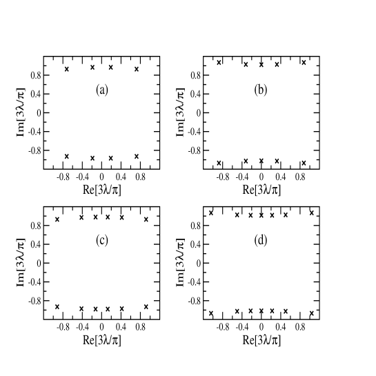
Figure 5: The ground state roots $z_{j}=\frac{3\lambda_{j}}{\pi}$ for (a) $L=8$, (b) $L=10$, (c) $L=12$, (d) $L=14$.

We then solve the Bethe equations (151) for larger values of $L$ to figure out the pattern of the roots in the thermodynamic limit $L\rightarrow\infty$. In Figure 6 we show the corresponding Bethe roots for $L=40~{}\mathrm{and}~{}42$. For better display of the roots curvature we shown the positive and the negative imaginary parts separately.

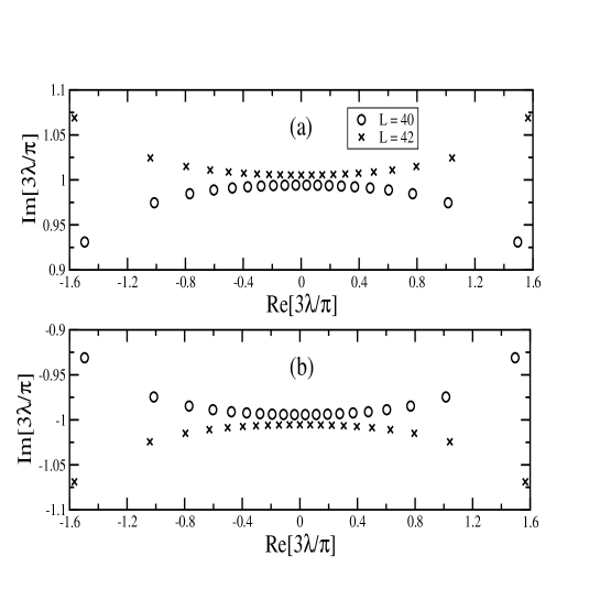
Figure 6: The ground state roots $z_{j}=\frac{3\lambda_{j}}{\pi}$ for $L=40$ and $L=42$ where (a) $z_{j}=x_{j}+iy_{j}$ and (b) $z_{j}=x_{j}-iy_{j}$.

The above analysis leads us to conclude that as $L\rightarrow\infty$ the roots $\lambda_{j}$ cluster in a complex $2-$strings. Each $2-$string has the same real part $\mu_{s}$ and equally spaced imaginary parts,

$$\lambda_{j}=\mu_{j}\pm\frac{i\pi}{3}~{},~{}\mu_{j}\in\mathbb{R}.$$ (153)

We now substitute the structure (153) in the Bethe equations (151) and by taking its logarithm we find that the resulting relations for $\mu_{j}$ are,

$$L\left[\phi\left(\mu_{j},\frac{5\pi}{12}\right)-\phi\left(\mu_{j},\frac{\pi}{4}\right)\right]=-2\pi Q_{j}+\sum_{k\neq j}^{n}\phi\left(2\mu_{j}-2\mu_{k},\frac{\pi}{3}\right)~{},~{}\text{for}~{}j=1,\ldots,n$$ (154)

where the function $\phi(x,y)=2\arctan[\tanh(x)\cot(y)]$ and $Q_{j}$ are integer or semi-integer numbers characterizing the logarithm branches.

Considering our numerical analysis we find that the low-lying spectrum can be described by the following sequence of $Q_{j}$ numbers,

$$Q_{j}=-\frac{1}{2}\left[\frac{L}{2}-n-1\right]+j-1~{},~{}\text{for}~{}j=1,\ldots,\frac{L}{2}-n.$$ (155)

For large $L$, the roots approach toward a continuous distribution with density $\rho(\mu)$ given by,

$$\rho(\mu)=\frac{d}{d\lambda}\left[Z_{L}(\mu)\right]$$ (156)

where the counting function is,

$$Z_{L}(\mu_{j})=\frac{1}{2\pi}\left[\phi\left(\mu_{j},\frac{\pi}{4}\right)-\phi\left(\mu_{j},\frac{5\pi}{12}\right)+\frac{1}{L}\sum_{k\neq j}^{L}\phi(2\mu_{j}-2\mu_{k},\frac{\pi}{3})\right].$$ (157)

Strictly in the $L\rightarrow\infty$, Eqs.(156,157) go into a linear integral equation for the density $\rho(\mu)$ which can be solved by standard Fourier transform method. The final result for $\rho(\mu)$ is,

$$\rho(\mu)=\frac{1}{\pi\cosh(2\mu)}.$$ (158)

The ground state energy per site $e_{\infty}$ can now be computed by taking the infinity volume limit of Eq.(152) and with the help of Eq.(158). By writing the result in terms of its Fourier transform we find,

$$e_{\infty}=\int_{0}^{\infty}d\omega\frac{\sinh[\frac{\pi\omega}{12}]-\sinh[\frac{\pi\omega}{4}]}{\cosh[\frac{\pi\omega}{4}]\sinh[\frac{\pi\omega}{2}]}=-\frac{2}{\pi}+\frac{\sqrt{3}}{9}.$$ (159)

Let us turn our attention to the behaviour of the low-lying excitations. These states are obtained from the Bethe equations (154) by introducing vacancies on the sequence of numbers $Q_{j}$. This method is by now standard to integrable models and for technicalities see for instance [23]. It turns out that the energy $\epsilon(\mu)$ and the momenta $\rho(\mu)$, measured from the ground state, of a hole excitation are given by,

$$\epsilon(\mu)=2\pi\rho(\mu)~{}~{}\text{and}~{}~{}\rho(\mu)=\int_{\mu}^{\infty}\epsilon(x)dx.$$ (160)

In order to calculate the low-lying dispersion relation $\epsilon(p)$ we have first to compute the integral in Eq.(160) and afterwards eliminate the variable $\mu$ from function $\epsilon(\mu)$. By performing these steps we find that the dispersion relation is

$$\epsilon(p)=2\sin(p).$$ (161)

From Eq.(161) we conclude that the low momenta excitations have a linear behaviour on the respective momenta. Therefore, the excitations are massless corroborating the connection between the geometric form of the curve and the nature of the spin-1 chain excitations made at end of section 4.

6 Conclusion

In conclusion, we have investigated the solutions of the Yang-Baxter equation for nineteen vertex models invariant by the action of parity-time reversal symmetry. We have developed a method to solve the corresponding functional equations from an algebraic point of view without the need of a priori spectral parameterization assumption. The structure of the algebraic manifolds constraining the Boltzmann weights follows a rather universal pattern allowing us to classify the possible integrable vertex models in four different families. They share the same fundamental algebraic curve which turns out to be a conic depending on three basic weights. By using the standard parameterization of conics we are able to obtain the dependence of the Boltzmann weights on the spectral parameter from a unified perspective. Three of such vertex models were already known before but the fourth model appears to be new in the literature.

We have observed an intriguing relation between the form of the main algebraic curve and the nature of the low-lying excitations of the related spin-1 chains. In the regime in which the geometric form of such curve is an ellipse the excitations are massless while when we have a hyperbolic structure the excitations have a mass gap. This fact is supported by previous knowledge on the physical properties of the first three spin-1 chains and also by the exact solution of the novel nineteen vertex model.

It seems interesting to investigate whether or not the scenario described above remains valid for other families of $\cal{PT}$ invariant vertex models with larger number of states. In principle, the systematic method developed here can be extended to tackle other models whose statistical configurations preserves at least one $U(1)$ symmetry. Another interesting problem is to study the algebraic invariants underlying vertex models that are not invariant by the $\cal{PT}$ symmetry and in particular to unveil the form of their principal algebraic curve. We hope to address these questions in future publications.

Appendix A: Three terms relations

This appendix is devoted to the presentation of some technical details entering the solution of the group $G_{\pm}^{(3)}$ relations. An immediate consequence of the last invariant (54) is that the weight $f^{(i)}$ can be easily written either in terms of the weights $a_{+}^{(i)}$ and $b_{+}^{(i)}$ or by means of the weights $a_{-}^{(i)}$ and $b_{-}^{(i)}$, namely

$$f^{(i)}=\frac{\left[a_{\pm}^{(i)}-\Gamma_{\pm}b_{\pm}^{(i)}\right]b_{\pm}^{(i)}}{\left(\Delta_{\pm}-\Gamma_{\pm}\right)a_{\pm}^{(i)}-b_{\pm}^{(i)}}~{}~{}\mathrm{for}~{}~{}i=1,2.$$ (A.1)

It turns out that Eq.(A.1) can be used to obtain a similar expression for the weight $d^{(i)}$. In fact, by substituting Eq.(A.1) in Eqs.(26,49,50) and by carrying on some simplification one finds,

$$\Lambda_{\pm}\left[d^{(i)}\right]^{2}=\frac{\left(1-\Delta_{\pm}\Gamma_{\pm}+\Gamma_{\pm}^{2}\right)\left[b_{\pm}^{(i)}\right]^{2}\left\{\left[a_{\pm}^{(i)}\right]^{2}-\Delta_{\pm}a_{\pm}^{(i)}b_{\pm}^{(i)}+\left[b_{\pm}^{(i)}\right]^{2}\right\}}{\left[\left(-\Delta_{\pm}+\Gamma_{\pm}\right)a_{\pm}^{(i)}+b_{\pm}^{(i)}\right]^{2}}~{}~{}\mathrm{for}~{}~{}i=1,2.$$ (A.2)

By using the form of the invariants $\Delta_{\pm}$ given by Eq.(22) in the expression (A.2) one is able to take the square root of the weight $\left[d^{(i)}\right]^{2}$. The final result is,

$$d^{(i)}=\pm\sqrt{\frac{1-\Delta_{\pm}\Gamma_{\pm}+\Gamma_{\pm}^{2}}{\Lambda_{\pm}}}\frac{b_{\pm}^{(i)}c_{\pm}^{(i)}}{\left(-\Delta_{\pm}+\Gamma_{\pm}\right)a_{\pm}^{(i)}+b_{\pm}^{(i)}}~{}~{}\mathrm{for}~{}~{}i=1,2.$$ (A.3)

This means that the compatibility among the invariants $\Gamma_{\pm}$ is equivalent to the matching of the expressions for the weights $f^{(i)}$ and $d^{(i)}$ coming from the distinct charge sectors $\pm$. By imposing such consistency one finds that Eq.(A.1) requires us to solve,

$$\left[\left(\Delta_{-}-\Gamma_{-}\right)a_{-}^{(i)}-b_{-}^{(i)}\right]\left[a_{+}^{(i)}-\Gamma_{+}b_{+}^{(i)}\right]b_{+}^{(i)}-\left[\left(\Delta_{+}-\Gamma_{+}\right)a_{+}^{(i)}-b_{+}^{(i)}\right]\left[a_{-}^{(i)}-\Gamma_{-}b_{-}^{(i)}\right]b_{-}^{(i)} = 0$$

$$\mathrm{for}~{}~{}i=1,2$$ (A.4)

while Eq.(A.3) implies that the compatibility for $d^{(i)}$ is,

$$\sqrt{\Lambda_{-}\left(1-\Delta_{+}\Gamma_{+}+\Gamma_{+}^{2}\right)}\left[\left(-\Delta_{-}+\Gamma_{-}\right)a_{-}^{(i)}+b_{-}^{(i)}\right]b_{+}^{(i)}c_{+}^{(i)}-$$

$$\sqrt{\Lambda_{+}\left(1-\Delta_{-}\Gamma_{-}+\Gamma_{-}^{2}\right)}\left[\left(-\Delta_{+}+\Gamma_{+}\right)a_{+}^{(i)}+b_{+}^{(i)}\right]b_{-}^{(i)}c_{-}^{(i)}=0~{}~{}\mathrm{for}~{}~{}i=1,2.$$ (A.5)

The analysis of Eqs.(Appendix A: Three terms relations,Appendix A: Three terms relations) for the index $i=1$ is immediate since the weights $a_{-}^{(1)}$ and $c_{-}^{(1)}$ are still free. Therefore, Eqs.(Appendix A: Three terms relations,Appendix A: Three terms relations) for $i=1$ are easily solved by eliminating the weights $a_{-}^{(1)}$ and $c_{-}^{(1)}$, namely

$$a_{-}^{(1)}=\frac{\Gamma_{-}(\Delta_{+}-\Gamma_{+})a_{+}^{(1)}b_{-}^{(1)}-a_{+}^{(1)}b_{+}^{(1)}-\Gamma_{-}b_{-}^{(1)}b_{+}^{(1)}+\Gamma_{+}\left[b_{+}^{(1)}\right]^{2}}{(\Delta_{+}-\Gamma_{+})a_{+}^{(1)}b_{-}^{(1)}-(\Delta_{-}-\Gamma_{-})a_{+}^{(1)}b_{+}^{(1)}-b_{-}^{(1)}b_{+}^{(1)}+\Gamma_{+}(\Delta_{-}-\Gamma_{-})\left[b_{+}^{(1)}\right]^{2}}b_{-}^{(1)}$$ (A.6)

and

$$c_{-}^{(1)}=\frac{-\sqrt{\Lambda_{-}(1-\Delta_{-}\Gamma_{-}+\Gamma_{-}^{2})(1-\Delta_{+}\Gamma_{+}+\Gamma_{+}^{2})}b_{-}^{(1)}b_{+}^{(1)}c_{+}^{(1)}}{\sqrt{\Lambda_{+}}\left\{(\Delta_{+}-\Gamma_{+})a_{+}^{(1)}b_{-}^{(1)}-(\Delta_{-}-\Gamma_{-})a_{+}^{(1)}b_{+}^{(1)}-b_{-}^{(1)}b_{+}^{(1)}+\Gamma_{+}(\Delta_{-}-\Gamma_{-})\left[b_{+}^{(1)}\right]^{2}\right\}}.$$ (A.7)

On the other hand the solution of Eqs.(Appendix A: Three terms relations,Appendix A: Three terms relations) for the index $i=2$ is more involving. This is the case because the weights $a_{-}^{(2)}$, $b_{-}^{(2)}$ and $c_{-}^{(2)}$ have already been determined in terms of the amplitudes $a_{+}^{(2)}$, $b_{+}^{(2)}$, $c_{+}^{(2)}$, $f^{(2)}$ and $d^{(2)}$ thanks to the previous relations (32,46). In addiction to that we also recall that the weights $f^{(2)}$ and $d^{(2)}$ are also determined in terms of $a_{+}^{(2)}$, $b_{+}^{(2)}$ and $c_{+}^{(2)}$ through Eqs.(A.1,A.3). Considering all these information together with the fact that the weight $\left[c_{+}^{(2)}\right]^{2}$ can be eliminated with the help of the invariant $\Delta_{+}$ (22) one concludes that Eqs.(Appendix A: Three terms relations,Appendix A: Three terms relations) are in fact a polynomial relation on the remaining weights $a_{+}^{(2)}$ and $b_{+}^{(2)}$. It turns out the expression of this polynomial associated to Eq.(Appendix A: Three terms relations), after using the constraints (35,45), is

$$B_{1}\left[a_{+}^{(2)}\right]^{3}+B_{2}a_{+}^{(2)}\left[b_{+}^{(2)}\right]^{2}+B_{3}\left[a_{+}^{(2)}\right]^{2}b_{+}^{(2)}+B_{4}\left[b_{+}^{(2)}\right]^{3}=0,$$ (A.8)

where its coefficients are given only in terms of the invariants values by,

$$B_{1} = \Psi[\Lambda_{+}^{2}\Gamma_{-}(-\Delta_{+}+\Gamma_{+})+\Lambda_{+}\Psi(\Delta_{+}\Gamma_{+}+\Gamma_{-}\Gamma_{+}-\Gamma_{+}^{2}+\Delta_{+}\Omega+\Gamma_{-}\Omega-\Gamma_{+}\Omega)$$ (A.9)

$$- \Psi^{2}(\Gamma_{+}^{2}+\Delta_{+}\Omega+2\Gamma_{+}\Omega+2\Omega^{2})],$$

$$B_{2} = \Lambda_{+}^{3}\Gamma_{+}(\Delta_{+}+2\Gamma_{-}-\Gamma_{+})+\Lambda_{+}^{2}\Psi(1-2\Delta_{+}\Gamma_{-}-\Delta_{+}\Gamma_{+}+\Gamma_{-}\Gamma_{+}-4\Gamma_{+}\Omega)+\Lambda_{+}\Psi^{2}(-1$$ (A.10)

$$- \Delta_{+}\Gamma_{-}+\Delta_{+}\Gamma_{+}-\Gamma_{-}\Gamma_{+}+\Delta_{+}^{2}\Gamma_{-}\Gamma_{+}+\Delta_{+}\Omega+\Gamma_{-}\Omega-\Gamma_{+}\Omega-\Delta_{+}^{2}\Gamma_{+}\Omega-\Delta_{+}\Gamma_{-}\Gamma_{+}\Omega$$

$$+ \Delta_{+}\Gamma_{+}^{2}\Omega-\Omega^{2}-\Delta_{+}\Gamma_{+}\Omega^{2}-2\Gamma_{-}\Gamma_{+}\Omega^{2}+\Gamma_{+}^{2}\Omega^{2})-\Psi^{3}(1-2\Delta_{+}\Gamma_{+}+\Gamma_{+}^{2}+\Delta_{+}^{2}\Gamma_{+}^{2}$$

$$- 2\Gamma_{+}\Omega+\Delta_{+}\Gamma_{+}^{2}\Omega+2\Omega^{2}-4\Delta_{+}\Gamma_{+}\Omega^{2}-4\Gamma_{+}\Omega^{3}),$$

$$B_{3} = -\Lambda_{+}^{3}(\Delta_{+}+\Gamma_{-}-\Gamma_{+})+\Lambda_{+}^{2}\Psi(\Gamma_{-}+\Delta_{+}^{2}\Gamma_{-}-\Gamma_{+}-\Delta_{+}\Gamma_{-}\Gamma_{+}+2\Omega)+\Lambda_{+}\Psi^{2}(\Delta_{+}+2\Gamma_{-}$$ (A.11)

$$- 2\Gamma_{+}-\Delta_{+}^{2}\Gamma_{+}-2\Delta_{+}\Gamma_{-}\Gamma_{+}+\Delta_{+}\Gamma_{+}^{2}-\Omega-\Gamma_{-}\Gamma_{+}\Omega+\Delta_{+}\Omega^{2}+\Gamma_{-}\Omega^{2}-\Gamma_{+}\Omega^{2})$$

$$+ \Psi^{3}(2\Delta_{+}\Gamma_{+}^{2}-3\Omega+4\Delta_{+}\Gamma_{+}\Omega+\Gamma_{+}^{2}\Omega-\Delta_{+}\Omega^{2}+2\Gamma_{+}\Omega^{2}-2\Omega^{3}),$$

$$B_{4} = -\Lambda_{+}^{3}\Gamma_{+}(1+\Gamma_{-}\Gamma_{+})+\Lambda_{+}^{2}\Psi(\Gamma_{-}-\Gamma_{+}+\Delta_{+}\Gamma_{+}^{2}+2\Gamma_{+}^{2}\Omega)+\Lambda_{+}\Psi^{2}(\Gamma_{-}-\Delta_{+}\Gamma_{-}\Gamma_{+}$$ (A.12)

$$+ \Gamma_{-}\Gamma_{+}^{2}-\Omega+\Delta_{+}\Gamma_{+}\Omega-\Gamma_{-}\Gamma_{+}\Omega+\Delta_{+}\Gamma_{-}\Gamma_{+}^{2}\Omega+\Gamma_{+}\Omega^{2}+\Gamma_{-}\Gamma_{+}^{2}\Omega^{2})-\Psi^{3}(\Omega-2\Delta_{+}\Gamma_{+}\Omega$$

$$+ \Gamma_{+}^{2}\Omega+\Delta_{+}^{2}\Gamma_{+}^{2}\Omega\Psi^{3}-2\Gamma_{+}\Omega^{2}\Psi^{3}+3\Delta_{+}\Gamma_{+}^{2}\Omega^{2}\Psi^{3}+2\Gamma_{+}^{2}\Omega^{3}\Psi^{3}).$$

As argued in the main text we are searching for solutions in which $a_{+}^{(2)}$ and $b_{+}^{(2)}$ are independent of each other. This means that we have to set all the coefficients of the polynomial (A.8) to zero. By imposing this condition for $B_{1}$ one is able to eliminate the invariant $\Gamma_{-}$ whose expression can be further simplified with the help of the constraint (36). The final result is,

$$\Gamma_{-}=\frac{\Psi}{\Lambda_{+}}\left(\Gamma_{+}+\Omega\right).$$ (A.13)

By substituting the result (A.13) in the expressions of the remaining coefficients (A.10-A.12) and by once again taking into account the constraint (36) we find that $B_{2}$, $B_{3}$ and $B_{4}$ vanish. The same reasoning can be repeated for Eq.(Appendix A: Three terms relations) when $i=2$. We conclude that it does not impose additional restriction besides Eq.(A.13).

We conclude by observing that the weights $a_{-}^{(i)}$, $b_{-}^{(i)}$ and $c_{-}^{(i)}$ can also be written in terms of the amplitudes $a_{+}^{(i)}$, $b_{+}^{(i)}$ and $c_{+}^{(i)}$. In order to see that we first substitute the weights $f^{(i)}$ e $d^{(i)}$, considering the index $+$ of Eqs.(Appendix A: Three terms relations,Appendix A: Three terms relations), in the expressions of the weights $b_{-}^{(1)}$, $b_{-}^{(2)}$, $c_{-}^{(2)}$, $a_{-}^{(2)}$, $a_{-}^{(1)}$ and $c_{-}^{(1)}$, see Eqs.(30,32,46,A.6,A.7). We next use the constraint $\Delta_{+}$ (22) to eliminate the amplitude $\left[c_{+}^{(i)}\right]^{2}$ besides the explicit form of the relations between the invariants (27,35,36,45,A.13). By performing such steps we are able to write rather simple expressions for the weights $a_{-}^{(i)}$, $b_{-}^{(i)}$, $c_{-}^{(i)}$ for $i=1,2$. They have given in the main text, see Eqs.(56-58).

Appendix B: Particular invariant solutions

We shall describe particular solutions for the invariants coming from branch 1A. Besides $\Psi=\Lambda_{+}=1$ we have two other possibilities that provide us non-null Boltzmann weights. We shall denominate such special branches as follows,

$$\bullet~{}~{}\mathrm{Branch~{}1S}:~{}~{}~{}\Psi=-\Lambda_{+}=1,$$ (B.1)

$$\bullet~{}~{}\mathrm{Branch~{}2S}:~{}~{}~{}\Psi=\Lambda_{+}=-1.$$ (B.2)

It turns out that the choices (B.1,B.2) lead us to the situation in which we do not have any free parameter at our disposal. In Table 5 we present the corresponding invariant values.

Invariants	Branch 1S	Branch 2S
$\Delta_{+}$	$\pm\sqrt{3}$	$\pm 2$
$\Delta_{-}$	$\mp\sqrt{3}$	$\pm 2$
$\Lambda_{+}$	$-1$	$-1$
$\Lambda_{-}$	$-1$	$-1$
$\Psi$	$1$	$-1$
$\Omega$	$0$	$0$
$\Gamma_{+}$	$\pm\frac{2}{\sqrt{3}}$	$\mp 1$
$\Gamma_{-}$	$\mp\frac{2}{\sqrt{3}}$	$\mp 1$
$\Theta_{+}$	$0$	$\pm 1$
$\Theta_{-}$	$\mp\frac{2}{\sqrt{3}}$	$0$
$\Delta_{+}^{(g)}$	$0$	$\pm 3$
$\Delta_{-}^{(g)}$	$0$	$\pm 3$
$\Delta_{+}^{(h)}$	$\pm\sqrt{3}$	$0$
$\Delta_{-}^{(h)}$	$\mp\sqrt{3}$	$0$
$\Delta_{+}^{(\tilde{h})}$	$\pm\sqrt{3}$	$0$
$\Delta_{-}^{(\tilde{h})}$	$\mp\sqrt{3}$	$0$

Table 5: Invariants values for the special branches 1S and 2S.

By comparing Table 5 with Table 2 it is not difficult to see that the branch 1S is a particular case of branch 1B once we choose $\Delta_{+}=\pm\sqrt{3}$. By the same token comparison with Table 3 reveals us that branch 2S becomes equivalent to branch 2A provided we set $\Delta_{+}=\pm 2$.

References

- [1] B.M. McCoy and T.T. Wu, Nuovo Cimento 56B (1968) 311; B. Sutherland, J.Math.Phys. 11 (1970) 3183; R.J. Baxter, Ann.Phys. 70 (1972) 193
- [2] R.J. Baxter, “Exactly Solved Models in Statistical Mechanics”, Academic Press, New York, 1982.
- [3] L.A. Takhtajan and L.D. Faddeev, Russ Math Sur. 34 (1979) 11; E.K. Sklyanin, L.A. Takhtadzhan and L.D. Faddeev, Ther. Math. Fiz. 40 (1979) 194
- [4] V.E. Korepin, G. Izergin and N.M. Bogoliubov, “Quantum Inverse Scattering Method and Correlation Functions”, Cambridge University Press, 1993
- [5] C.S. Melo and M.J. Martins, Nucl. Phys. B 806 (2009) 567
- [6] P.W. Kasteleyn, Fundamental Problems in Statistical Mechanics, North-Holland, Amsterdam, vol. 3, 1975.
- [7] I.M. Krichever, Funct. Anal. Appl. Math. 15 (1981) 92
- [8] W. Galleas and M.J. Martins, Phys. Rev. E 66 (2002) 047103
- [9] T.T. Wu and B. McCoy, Nuovo Cimento 56B (1968) 311; B. Sutherland, C.N. Yang and C.P. Yang, Phys. Rev. Letters 19 (1967) 588
- [10] R.J. Baxter, Ann. Phys. 70 (1972) 193; 71 (1973) 1
- [11] C. Fan and F.Y. Wu, Phys. Rev. B 2 (1970) 723; B.U. Felderhof, Physica 66 (1973) 279; 66 (1973) 509
- [12] A.B. Zamolodchikov and V.A. Fateev, Sov. Nucl. Phys. 32 (1980) 298
- [13] A.G. Izergin and V.E. Korepin, Commun. Math. Phys. 79 (1981) 303
- [14] T. Deguchi and Y. Akutsu, J. Phys. Soc. Jpn. 60 (1991);Mod. Phys. Lett. A7 (1992) 767
- [15] M. Couture, J. Phys. A: Math. Gen. 24 (1991) L103
- [16] C. Gomez, M. Ruiz-Altaba and G. Sierra, Phys. Lett. B 265 (1991); C. Gomez and G. Sierra, Nucl. Phys. B 373 (1992) 761
- [17] M. Idzumi, T. Tokihiro and M. Arai, J.Phys.I France 4 (1994) 1151
- [18] F.C. Alcaraz and R.Z. Bariev, J.Phys.A:Math.Gen. 34 (2001) 1467; F.C. Alcaraz and M.J. Lazo, J.Phys.A:Math.Gen. 37 (2004) 4149
- [19] H.M. Babujian and A.M. Tsvelick, Nucl.Phys.B 265 (1986) 24
- [20] H.J.de Vega and E. Lopes, Nucl.Phys.B 362 (1991) 261
- [21] S.O. Warnaar, M.T. Batchelor and B. Nienhuis, J.Phys.A:Math.Gen. 25 (1992) 3077
- [22] A. Berkovich, C. Gomez and G. Sierra, J.Phys.A:Math.Gen. 26 (1993) L45
- [23] B. Sutherland, Phys. Rev. B. 12 (1975) 3795; L.D. Faddeev and L. Takhtajan, Phys. Lett. A 85 (1981) 375