New insight on galaxy structure from GALPHAT i@. Motivation, methodology, and benchmarks for Sérsic models

Abstract

We introduce a new galaxy image decomposition tool, Galphat (GALaxy PHotometric ATtributes), which is a front-end application of the Bayesian Inference Engine (BIE), a parallel Markov chain Monte Carlo package, to provide full posterior probability distributions and reliable confidence intervals for all model parameters. The BIE relies on Galphat to compute the likelihood function. Galphat generates scale-free cumulative image tables for the desired model family with precise error control. Interpolation of this table yields accurate pixelated images with any centre, scale, and inclination angle. Galphat then rotates the image by position angle using a Fourier shift theorem, yielding a high speed and accurate likelihood computation.

We benchmark this approach using an ensemble of simulated Sérsic model galaxies over a wide range of observational conditions: the signal-to-noise ratio S/N, the ratio of galaxy size to the PSF and the image size, and errors in the assumed PSF; and a range of structural parameters: the half-light radius $r_{e}$ and the Sérsic index $n$. We characterise the strength of parameter covariance in Sérsic model, which increases with S/N and $n$, and the results strongly motivate the need for the full posterior probability distribution in galaxy morphology analyses and later inferences.

The test results for simulated galaxies successfully demonstrate that, with a careful choice of Markov chain Monte Carlo algorithms and fast model image generation, Galphat is a powerful analysis tool for reliably inferring morphological parameters from a large ensemble of galaxies over a wide range of different observational conditions.

1 Introduction

The formation and evolution of galaxies is an outstanding problem in Astronomy and galaxy morphology remains a key observational attribute in the quest to increase our understanding of galaxy evolution. The increasing sensitivity and resolution of planned surveys will enable tests of evolution theories from the epoch of formation to the present. However, selection effects and features peculiar to one’s choice of models will affect any interpretation. Therefore, to exploit the promise of survey data, we need to verify that our conclusions are reliable. The tools described in this paper are a step in this direction.

Early $\Lambda$CDM hierarchical galaxy formation theory and simulations placed galaxies in the Hubble sequence by following a combination of merger histories and gas accretion (White & Frenk, 1991; Steinmetz & Navarro, 2002). Later, “zoom-in” resimulations of individual galaxies have produced more realistic galaxy morphologies (Abadi et al., 2003a, b; Sommer-Larsen et al., 2003; Governato et al., 2004; Robertson et al., 2004; Zavala et al., 2008). Although challenging, combinations of semi-analytic models and direct simulations (Benson & Devereux, 2010; Croft et al., 2009; Parry et al., 2009; Scannapieco et al., 2010) have quantified the distribution of galaxy morphology with redshift.

These recent theoretical studies have been motivated by large-scale spectroscopic and image surveys. In the local Universe, millions of galaxies have been detected in the Sloan Digital Sky Survey (SDSS, York et al., 2000) and the Two Micron All Sky Survey (2MASS, Skrutskie et al., 1997; Skrutskie, 2006). Recent analyses have used a range of models from single-component Sérsic profiles (Sérsic, 1963) to more sophisticated bulge and disc-bar models to characterise the structural properties of local galaxy morphology (Blanton et al., 2003; Allen et al., 2006; Gadotti, 2009). In the more distant Universe, COSMOS (Scoville et al., 2007) provides an ample collection of multi-wavelength galaxy images and spectroscopy to study the evolution of galaxy morphological structure for $z\la 1$ as a function of mass and environment (Capak et al., 2007; Cassata et al., 2007; Kovač et al., 2010). Gas accretion, disc instability, mergers, and supernova and black hole feedback have been modelled to explain morphological evolution and it is possible to assess their relative importance by quantitatively comparing observed galaxy morphological structures to those predicted from theory. Furthermore, future large-scale multi-band imaging surveys, such as the Large Synoptic Survey Telescope (LSST Science Collaboration, 2009), combined with accurate photometric distances will provide a uniform and consistent data set to study the evolution of the galaxy population.

Algorithmic approaches to measure galaxy morphology are recent inventions and are usually based on mixture models of parametric surface brightness distributions (Byun & Freeman, 1995; Simard, 1998; Wadadekar et al., 1999; Peng et al., 2002; Simard et al., 2002; MacArthur et al., 2003; de Souza et al., 2004; Pignatelli et al., 2006; Méndez-Abreu et al., 2008). However, systematic biases owing to an ignorance of uncertainties in the sky background and covariances between model parameters complicate their interpretation. To circumvent these difficulties, we advocate embedding the galaxy morphology analysis into the broader context of inference and hypothesis testing. In this paper, we present such a Bayesian approach using the Markov chain Monte Carlo (MCMC) technique, facilitated by embedding it within the Bayesian Inference Engine (BIE, Weinberg & Moss, 2010). To motivate this approach, we first illustrate the inherent difficulties in galaxy image decomposition in §§1.1–1.2.

1.1 Case studies

The following three examples explore the limitations of conventional model fitting and the improvements gained using Bayesian inference when inferring the photometric attributes of galaxies.

1.1.1 Posterior distributions versus best-fit parameters

We pick two galaxies from our pool of Sérsic profile simulated galaxy images (see § 1.1.2). One has a high signal-to-noise ratio, S/N$=100.01$, and the other has a low signal-to-noise ratio, S/N$=10.46$. The value of S/N is defined by the ratio of the galaxy signal to the noise within the half-light radius (see §4.1). Since we know the Sérsic model parameter values used to generate these galaxy images, we fix all parameters to their true values, except for the Sérsic index $n$, and calculate the $\chi^{2}$ likelihood for different values of $n$.

(a) Likelihood

(b) Posterior probability

Figure 1: Panel (a): the likelihood as a function of Sérsic index $n$ for two example galaxies with different S/N. Each likelihood value is normalised to the maximum. The distribution for the high S/N galaxy (upper) is sharply-peaked and the distribution for low S/N galaxy (lower) is broadly-peaked. Panel (b): the posterior probability density of $n$ for the two galaxies. The black dot with error bar is the best-fit parameter from Galfit (Peng et al., 2002). The shaded region is the 68.3% confidence interval and the vertical dotted line is the true value of $n$. The conventional error estimate based on the second derivative of the likelihood is much too large for low S/N.

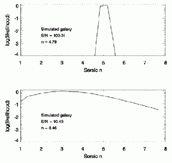
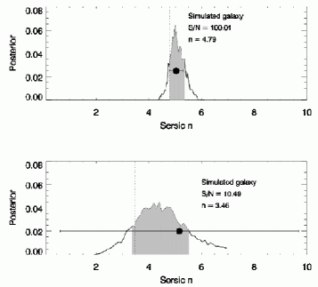
Figure 1a shows the likelihood as a function of $n$ for each galaxy. The upper panel plots the high S/N galaxy and the lower panel the low S/N one. For the high S/N galaxy the likelihood has a very strong mode around $n=5$ with a change by factor of 4 in log, as $n$ varies from 4.5 to 5.5. However, for the low S/N galaxy the likelihood is very broad, smoothly changing by 0.4 in log as $n$ varies from 3 to 5, and the likelihood profile is not symmetric around the maximum. In addition, the precise location of the global maximum is not informative; a local analysis of the profile using standard inverse-Hessian analysis would not give an accurate estimate of the profile shape. Finally, in general, a typical multi-dimensional likelihood surface will have an even more complex landscape.

Figure 1b shows the posterior probability of each galaxy’s $n$ for the given data, marginalised over the other parameters as computed by Galphat. The solid curve is the posterior probability of $n$ and the shaded region corresponds to a 68.3% confidence interval. The true value is indicated by the vertical dotted line, and the error bar shows the result using Galfit (Peng et al., 2002). Galfit is a widely-used galaxy image decomposition program, based on a maximum likelihood (ML) approach, implemented as a $\chi^{2}$ minimisation using the Levenberg-Marquardt algorithm (Press et al., 1998). The posterior mode of $n$ is offset from the true value by 0.2 for the high S/N galaxy and by 1.0 for the low S/N galaxy. Such a bias always occurs owing to random photon counting errors. Although the bias is large for low S/N, each 68.3% confidence interval of $n$ encloses the true value. The best-fit value of $n$ from Galfit for the high S/N galaxy is close to the posterior mode and the associated error bar, corresponding to a 68.3% confidence interval, encloses the true value. However, for the low S/N galaxy the best-fit parameter from Galfit, using its simple minimisation algorithm, is more subject to small-scale variations of the likelihood profile owing to sampling and the best-fit parameter may also depend on the initialisation of the downhill solver. Furthermore, the inverse-Hessian estimate of the variance in one dimension is simply the inverse of the second derivative of the likelihood; geometrically, the faster the slope varies with $n$, the smaller the variance. This makes the error reported by Galfit unrealistically large because there is no significant variation in the tangent slope at the best-fit value of $n=5.16$. A reliable error estimate is crucial to quantifying trends in the derived properties of galaxies. The Bayesian MCMC approach adopted here samples the full posterior distribution and yields reliable error estimates of each model parameter given the data. Hence, this provides a solid statistical base for an analysis of galaxy morphology.

1.1.2 Bias and prior assumptions

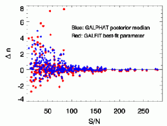
We now explore the distribution of the best-fit $n$ for 325 galaxies with their Sérsic model index $n$ sampled from a normal distribution $n\sim\mathcal{N}(4.0,0.33^{2})$. Figure 2a plots the residual value of the $n$ using the posterior median of $n$ from Galphat (blue diamonds) with a uniform prior for $n\sim\mathcal{U}(0.2,10.0)$ and the best-fit value from Galfit (red circles). For the Galfit estimates, we used the true values as the centroids of the distribution for the initial guess and randomly perturbed the magnitude, galaxy radius $r_{e}$, axis ratio, position angle, and sky background by $\pm 0.5$, $\pm 20\%$, $\pm 10\%$, $\pm 15\%$ and $\pm 1\%$, respectively, about these true values, assuming a uniform distribution within these ranges. In Galphat we assumed uniform priors for these parameters within these same ranges. The initial Galfit guess for the Sérsic index is $n=2.5$ for all the galaxies. As an image’s S/N decreases, the variance in the residual value of $n$ becomes larger and $n$ becomes preferentially overestimated owing to the asymmetric shape of the likelihood profile (see Fig. 1). For low S/N, the Galfit values are sensitive to the initial guess in contrast to Galphat, which samples the parameter space using MCMC and hence is insensitive to the initial guess. The variance in the best-fit $n$’s from Galfit is slightly larger than the variance in the Galphat posterior medians owing to its insufficient accuracy in finding the correct global likelihood minimum for low S/N data.

(a) Uniform prior distribution

(b) Non-uniform prior distribution

Figure 2: The distribution of residual Sérsic index $n$ for 325 galaxies with $n\sim\mathcal{N}(4.0,0.33^{2})$. Panel (a): Galphat posterior median values (blue diamonds) and best-fit Galfit values (red circles). Galphat uses uniform priors with the same parameter range used in Galfit for a fair comparison. Panel (b): same as (a) but with a non-uniform prior for $n$ in Galphat. The prior distribution has a $\sigma$ roughly 13 times larger than the input distribution. By introducing an informative prior, the parameter recovery is significantly improved with decreasing S/N.

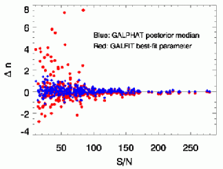
However, if we allow parameters to have an informative prior distribution, the Galphat-derived posterior distribution improves dramatically (Fig. 2b). We use a Weibull distribution for the prior probability of $n$ with $\lambda=7.0$ and $k=1.5$, whose deviation ($\sigma=4.3$) from the mean is still 13 times larger than the deviation of the true distribution but embodies our astronomical experience from the literature. The variance in the posterior median of the residual of $n$ for low S/N images decreases significantly. With an appropriately chosen prior distribution, the Bayesian approach can dramatically increase the quality of the inference over the entire input catalogue. Many people have aesthetic objections to the Bayesian approach, because they view the selection of a prior as being subjective and, therefore, arbitrary. The statistics and astrostatistics literature abound with philosophical discussions of this issue. It is our point of view that prior information will be used by a researcher inevitably, so why not let the Bayes theorem tell us how to use it quantitatively? Conversely, wholesale adoption of uniform priors, e.g. in the maximum likelihood method, is both arbitrary and self-defeating, since we know that most parameters have both physical constraints and previously measured distributions. In other words, ignoring one’s own expert opinion is daft.

These issues are less significant for data with high S/N. However, astronomical surveys have widely-ranging S/N values, and the total number of galaxies for flux-limited samples will always be dominated by images with low or moderate S/N. Therefore, improving our estimates of structural parameters in the low S/N regime best uses the available data and optimises scientific return.

1.1.3 Scatter plots versus joint posterior distributions

Here we explore the joint distribution of galaxy half-light radius $r_{e}$ and Sérsic index $n$ for the same galaxy image sample from the last sub-section. Figure 3a is a conventional scatter plot showing the joint distribution of best-fit values of $r_{e}$ and $n$ from Galfit. Figure 3b shows the joint posterior distribution of $r_{e}$ and $n$ from Galphat. The contour levels are the 30, 50, 68.3 (green line), 95, and 99% confidence values (white to black). Since the galaxy sample is generated without any correlations between $r_{e}$ and $n$, we should not see any covariance between $r_{e}$ and $n$. Comparing these two panels, the scatter plot from Galfit shows a (spurious) systematic trend of $n$ with $r_{e}$ while the joint posterior distribution from Galphat does not. Some Sérsic-model parameters, e.g. $r_{e}$ and $n$, are reported to exhibit a true covariance (Trujillo et al., 2001), so such systematic trends in the distribution of best-fit parameters as exhibited by Galfit will obscure or contaminate any intrinsic covariance.

(a) Scatter plot

(b) Posterior distribution

Figure 3: The joint distribution of galaxy half-light radius $r_{e}$ and Sérsic index $n$ for 325 galaxies. The simulated galaxies were generated without any correlation between $r_{e}$ and $n$. Panel (a) shows the conventionally used scatter plot using the best-fit model parameter from Galfit and Panel (b) shows the joint posterior of $r_{e}$ and $n$ from Galphat with 30, 50, 68.3 (green line), 95 and 99% confidence level (white to black).

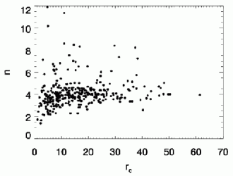
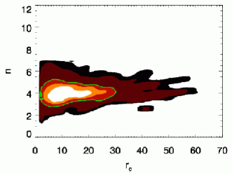
The qualitative difference between the Maximum Likelihood (ML)-inferred scatter plot and the Bayesian-inferred joint posterior underlines our assertion that understanding parameter covariance, the use of thoughtful prior distributions, and a thorough error analysis are essential to reliably testing hypotheses based on the morphologies of a large number of galaxies. Even so, the choice of a parametric family induces a correlation between parameters and, therefore, a single “best-fit” value does not adequately characterise the knowledge acquired from the data. Examples and conclusions such as these motivate our using the entire posterior distribution in parameter space for all of the galaxies that we wish to study.

1.2 Bayesian MCMC to the rescue

The main disadvantage of the Bayesian approach is its computational expense. Over the last 15 years, MCMC techniques have continued to improve and we believe that these techniques are now suitable as mainstream tools. Here, we introduce a computationally-tractable Bayesian MCMC approach that overcomes the difficulties outlined in the previous sections. Significant improvement over previous attempts to understand galaxy evolution using morphology can be achieved using a Bayesian approach for the following three reasons:

1. The ML method assigns the best-fit parameter value to the model that has the highest probability of generating the observed data. With sufficient data, this yields the correct result (assuming that some model in the family generates the data). However, Nature gives us one realization of a particular galaxy and this leads to competing models that can generate the same data through different processes. Rather than the ML question, we want to know the best model among the possible candidates, or what is the probability of the model for the observed data? Written in the language of conditional probability, this question gives us Bayes theorem and requires an estimate of the probability of the model before acquiring the data (the prior probability). The Bayesian formulation of the inference problem provides a natural foundation for Astronomy, where every single event is unique and observers can not test theories by changing the initial conditions of the Universe. If data has high S/N and strongly supports a particular model, the inference should not be subject to the bias introduced by the prior distribution. Conversely, if data has low S/N, the inference may be influenced by the prior assumptions, as intuitively expected.

2. We have seen that inferences based on best-fit analyses can be contaminated by intrinsic covariance in the chosen model family. In addition, the topology of the likelihood function in a high-dimensional parameter space with a large number of free parameters is very complex in general. Therefore, one needs to both find the true global extremum and assess the significance of this extremum with respect to nearby and possibly unanticipated extrema in the probability space. Bayesian MCMC provides the full posterior and the confidence levels of inferences for each model parameter. Hence one can investigate correlations or perform hypothesis tests with quantifiable confidence.

3. The adoption of specific functional families, e.g. Sérsic profiles, may not provide an adequate explanation for the observed data or have sufficient power to classify differences between data sets. In the Bayesian paradigm, one may consistently assess the explanatory power of different models even if they are not nested. For example, one may rigorously pose the question “how strongly is the assumption of a single-component Sérsic model supported by the galaxy image data compared to a two-component bulge and disc model?” This provides a natural way of probabilistically classifying galaxies.

To summarise, our Bayesian approach uses galaxy morphology as an intermediate step in an overall inference problem for theories of galaxy evolution. In contrast, by focussing on the best-fit parameters as the data-reduction goal, and comparing the implied correlations to those predicted by theories of galaxy formation, one runs the risk of interpreting false correlations and one decreases the information content of one’s data by using only the best-fit parameter as a summary value. Motivated by the promise of dramatic improvement, we have developed a novel image decomposition software package, Galphat (GALaxy PHotometric ATtributes), based on a Bayesian Markov chain Monte Carlo approach. The general application to astronomical image analysis is not new: Bayesian MCMC has been used for X-ray surface brightness estimation of galaxy clusters (Andreon et al., 2008), for object detection (Carvalho et al., 2009; Guglielmetti et al., 2009; Hobson & McLachlan, 2003; Savage & Oliver, 2007), for dynamical modelling of a galaxy (Puglielli et al., 2010), and for gravitational weak lensing (Kitching et al., 2008; Miller et al., 2007) and strong lensing analyses (Vegetti & Koopmans, 2009). Galphat is designed for performing morphological analysis of galaxy images similar to several widely-used galaxy image decomposition packages such as: BUDDA (de Souza et al., 2004), Galfit (Peng et al., 2002), Gasp2d (Méndez-Abreu et al., 2008), Gasphot (Pignatelli et al., 2006) and Gim2d (Simard et al., 2002; Simard, 1998), but has a firm probabilistic foundation, providing full posterior distributions of the parameters, which are suitable for a variety of inference problems such as model comparison, hypothesis testing, and correlation analyses.

One of our original motivations for developing Galphat is the large scale analysis of galaxy morphological structures in 2MASS (Skrutskie et al., 1997; Skrutskie, 2006). The interpretation of 2MASS-galaxy properties has suffered from using unreliable best-fit parameters obtained using conventional fitting algorithms. An ensemble of posterior distributions for a complete sample of local galaxies becomes a rich database for hypothesis testing in two ways. First, we may characterise the distributions of galaxy morphological structures, e.g. the luminosity, the size and the shape, as a function of environment, with rigorous statistical confidence levels. Secondly and more generally, we may compare galaxy formation theories based on the morphological evidence.

This paper introduces Galphat and emphasises methods, features and performance issues. We demonstrate the feasibility of a large-scale statistical inference based on galaxy morphology. A more detailed exploration of the influence of the prior distribution, explicit examples of model comparisons between single Sérsic and two-component bulge and disc models, and inferences using an ensemble of posterior distributions will be reported in a followup paper (Yoon et al., 2010). The paper is organised as follows. In §2, we describe the basic formalism of Bayesian inference for galaxy image data and introduce the Bayesian Inference Engine (BIE), which is used to sample the posterior distributions of model parameters. We describe the structure of Galphat in §3 and our ensemble of simulated galaxy images for calibrating Galphat in §4. Comprehensive test results are presented in §5. We summarise our findings and conclusions in §6.

2 Bayesian Markov chain Monte Carlo

2.1 Theoretical background

Bayes theorem states that the probability of a model characterised by its parameter vector $\theta$, given some data set $D$, is proportional to the likelihood of the data for the given model multiplied by the prior probability of the model

$$P(\theta|D)=\frac{L(D|\theta)\pi(\theta)}{\int L(D|\theta)\pi(\theta)d\theta}$$ (1)

where $P(\theta|D)$ is the posterior distribution, $L(D|\theta)$ is the likelihood function, i.e. the probability of the data given $\theta$, and $\pi(\theta)$ is the prior distribution of the parameter vector $\theta$. If $\pi(\theta)$ is a uniform distribution in a compact subset of $\mathbb{R}^{n}$, we recover the ML method.

The goal is to characterise the posterior distribution by sampling $P(\theta|D)$. For simple cases with a few model parameters, one can analytically calculate it or explore the probability space by evaluating the posterior probability over a grid in parameter space. However, for our Sérsic model with 8 parameters this approach is not feasible. Fortunately, owing to the rapid improvement in computational methodology, MCMC is feasible in high-dimensional parameter spaces. MCMC generates states by a first-order Markovian process and the distribution of states asymptotically converges to the target distribution $P(\theta|D)$ after a large number of iterations.

For the model selection problem, one may apply Bayes theorem to give the probability of the theory $M$ based on the data $D$ given a prior probability of the theory. In our case, $M$ is the assumption of a particular model family with a parameter vector $\theta$, e.g. the theory that galaxies are Sérsic models. The likelihood of a theory is the probability of the data given the theory. Algebraically, the probability of the data given the theory is the marginalisation of the likelihood function over the prior probability of the model parameter distribution: $P(D|M)=\int L(D|M,\theta)\pi(\theta|M)d\theta$. This quantity is a measure of how well the evidence supports the theory. In other words, the more probable the evidence given the theory, the more the evidence supports the theory. Of course, one needs to know what the theory predicts to know how well the evidence supports it and this is the job of the MCMC simulation. Now, let $P(M)$ be the prior probability of the theory. Then, analogous to the Bayes theorem from equation (1), we may write the probability of the theory given the data as

$$P(M|D)=\frac{P(D|M)P(M)}{\int P(D|M)P(M)\,dM}.$$ (2)

Equation (2) immediately gives an estimate of the posterior odds of two different theories $M_{1}$ and $M_{2}$ parametrised by different parameter vectors $\theta_{1}$ and $\theta_{2}$:

$$\frac{P(M_{1}|D)}{P(M_{2}|D)}=\frac{P(M_{1})}{P(M_{2})}K_{12}\quad\mbox{where}\quad K_{12}\equiv\frac{P(D|M_{1})}{P(D|M_{2})}.$$ (3)

The quantity $K_{12}$ is called the Bayes factor. The numerator and denominator of $K_{12}$, $P(D|M_{i})$, is called the marginal likelihood for model $i$. If one does not favour one of the two theories a priori, the term $\frac{P(M_{1})}{P(M_{2})}=1$ since $P(M_{1})=P(M_{2})$. Therefore, the Bayes factor describes the increase of odds in favour of one theory over another in the light of the data. The Bayesian model comparison does not depend on the particular parameters used by each model. Instead, it considers the probability of the model considering all possible parameter values.

However, it should be clear from equation (2) that the Bayes factor depends on the choice of the prior distribution. If the likelihood dominates, the effect of the prior is negligible, but if the prior contributes to the posterior significantly as well as the likelihood, an incorrect prior leads to a biased inference (e.g. Kass, 1993). The choice of prior must be considered carefully. The effects of prior choice on Galphat will be addressed in detail in our follow-up paper (Yoon et al., 2010).

2.2 The Bayesian Inference Engine (BIE)

The ability to realise the promise of this approach depends on an accurate computation of the posterior distribution. Although the Markov chain will approach its steady-state distribution almost certainly, the number of steps required, the mixing time, is not known. In addition, the exploration of parameter space suffers from the curse of dimensionality. We need assurance that the Markov chain is in a steady state beyond the local region in parameter space. For example, consider a posterior distribution with discrete, separated modes; many chains will not be able to move between these modes, resulting in an infinite mixing time and an incomplete posterior distribution.

Various MCMC algorithms have been proposed to improve the convergence of MCMC, and each of these have their own advantages and disadvantages. Beginning in 2000, a multi-disciplinary investigator team from the Departments of Astronomy and Computer Science at the University of Massachusetts designed and implemented the Bayesian Inference Engine, a MCMC parallel software platform for performing statistical inference over very large data sets. The BIE uses a scalable multiprocessor software architecture designed to operate on modest cost, generally available hardware. MCMC algorithms and Bayesian computation in general are ideally suited to multiprocessor computation. The BIE uses standard MPI and POSIX threads and, therefore, will run in a broad spectrum of parallel or scalar environments and can be easily ported to high-performance hardware for production analysis. Fundamentally, the BIE is a library, but the package provides a command-line interpreter (CLI) with access to nearly all of the import object classes. This CLI was originally intended for interactive or script-based prototyping with subsequent stand-alone hard-coding. However, most users simply use the CLI with scripts. The BIE’s object-oriented design allows a researcher to apply a wide variety of MCMC algorithms to the same target application by changing several lines in a program or script. The BIE currently includes: the standard Metropolis-Hastings algorithm (Hastings, 1970; Metropolis et al., 1953), the simulated tempering algorithm (Neal, 1996), the parallel tempering algorithm (Geyer, 1991), the parallel hierarchical sampler (Rigat, 2008, PHS hereafter), the differential evolution algorithm (Braak, 2006), and an independent multiple chain algorithm. For convergence testing, the BIE implements the algorithm proposed by Giakoumatos et al. (Giakoumatos et al., 1999) for single-chain simulations and the Gelman-Rubin (Gelman & Rubin, 1992) convergence diagnostic for multiple-chain simulations.

The object-oriented design makes the BIE extensible; new MCMC algorithms, new convergence algorithms, and new models or likelihood functions can be implemented and added to the BIE at any time. For example, a typical user will typically develop new models for a specific scientific problem. At a later time, the user may use a newly available MCMC algorithm without changing this model code. Since MCMC computations are computationally expensive, the BIE provides a full serialisation and persistence system. This system saves the entire state of all the objects in the simulation. For example, the BIE automatically saves checkpoint images. Therefore, Galphat can restart from the very last MCMC step to sample the posterior further for obtaining more MCMC samples when needed, significantly saving computational resources. Moreover, the results of previously performed simulations can be restored on the fly and compared or reused in new ways. See Weinberg & Moss (2010) for additional details.

3 GALPHAT: algorithms and features

Galphat is implemented as a user-contributed likelihood function to the BIE. It reads two-dimensional galaxy image data from a FITS file, generates a model image, and then computes the likelihood. Because the posterior simulation requires a large number of likelihood evaluations, optimisation of the model image generation is essential to make the analysis of an entire image catalogue feasible. In this section, we describe the implementation details and features of Galphat.

3.1 Overview of our Galphat  implementation

The BIE controls the MCMC algorithm, the convergence testing, and logging the sampled posterior distribution. As needed, the BIE requests a likelihood evaluation from Galphat. The flow chart for Galphat is as follows:

1. Galphat reads the input FITS files (the galaxy image and the PSF) and the tabulated model images (see below) for later interpolation.

2. As part of the MCMC simulation, the BIE calls the likelihood function with a parameter vector. Using these parameters, Galphat interpolates and scales the image table using the scale radius and the minor/major axis ratio, and generates a model image in principle-axis coordinates.

3. Galphat convolves the model image with input PSF image in Fourier space using the FFTW package and adds the sky background.

4. Finally, the model image is rotated by the position angle, using a Fourier shift algorithm, in pixel coordinates.

5. Galphat returns the likelihood evaluation to the BIE.

6. Steps (ii)–(v) are repeated as necessary.

We will describe the details for each important step below.

3.2 Model generation

Any symmetric galaxy model has six model-independent free parameters: the centroid coordinates $(x,y)$, the axis ratio $q=b/a$, the position angle, the scale length, and the total flux or magnitude. For tests in this paper, we use a Sérsic model (Ciotti, 1991; Graham & Driver, 2005; Sérsic, 1968). The Sérsic model is a one-parameter model family described by the index $n$. As the index increases, the profile increases in concentration: an exponential disc profile has $n=1$ and a de Vaucouleur profile has $n=4$. The model has the following analytic form

$$\Sigma(r)=\Sigma_{e}\mbox{exp}\left[-\kappa\left\{\left(\frac{r}{r_{e}}\right)^{1/n}-1\right\}\right]$$ (4)

where the effective radius, $r_{e}$, defines a scale length. By construction $r_{e}$ is equivalent to the half-light radius, $r_{50}$. The quantities $\kappa$ and $n$ are related through the relation

$$\Gamma(2n)=2\gamma(2n,\kappa)$$ (5)

where $\Gamma$ is the complete gamma function and $\gamma$ is the incomplete gamma function. Approximate analytic expressions for $\kappa$ can reduce the computation time. For $n>0.36$ we adopt the following asymptotic expansion for $\kappa$, which is good to better than one part in $10^{4}$ (Ciotti & Bertin, 1999; MacArthur et al., 2003):

$$\kappa\approx 2n-\frac{1}{3}+\frac{4}{405n}+\frac{46}{25515n^{2}}+\frac{131}{1148175n^{3}}-\frac{2194697}{30690717750n^{4}}+O(n^{-5}).$$ (6)

For $n\leq 0.36$, we use the following polynomial fit (MacArthur et al., 2003), accurate to better than two parts in $10^{3}$:

$$\kappa\approx 0.01945-0.8902n+10.95n^{2}-19.67n^{2}+13.43n^{3}.$$ (7)

(a) Surface brightness profile

(b) Cumulative flux

Figure 4: Panel (a): Sérsic surface-brightness profiles for n=0.5, 1, 2, 4 and 8 (eq. 4). The profiles are normalised to have equal flux density at $r=r_{e}$. Panel (b): the fraction of light within $r$ for Sérsic profiles with n=0.5, 1, 2, 4 and 8. For $n=8$, a few percent of the flux has $r>100r_{e}$!

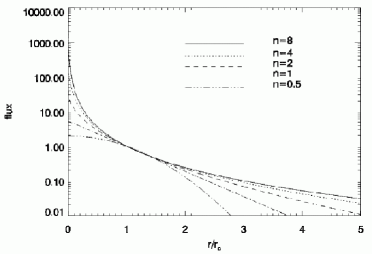
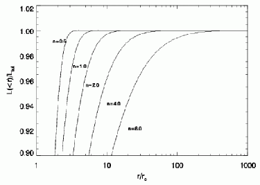
Figure 4a shows Sérsic profiles with different $n$, normalised to have equal fluxes at $r_{e}$. As $n$ increases, the central profile steepens and the wings thicken. The luminosity within a radius $r$ is

$$L(<r)=\Sigma_{e}2\pi r_{e}^{2}qn\frac{e^{\kappa}}{\kappa^{2n}}\gamma(2n,x)$$ (8)

where $x=\kappa(r/r_{e})^{1/n}$ (Graham & Driver, 2005). Replacing $\gamma(2n,x)$ with $\Gamma(2n)$ gives the total luminosity $L_{tot}$ (Ciotti, 1991; Ciotti & Bertin, 1999; Graham & Driver, 2005).

The fraction of light within $r$ for different values of $n$ is shown in Figure 4b. As summarised in Graham & Driver (2005), for an exponential disc (i.e. $n=1$) profile, 99.1% and 99.8% of the flux is within the inner $4r_{e}$ and $5r_{e}$, respectively. For a de Vaucouleur profile (i.e. $n=4$), 84.7% and 88.4% of the flux is within the inner $4r_{e}$ and $5r_{e}$, respectively. The sky background and index $n$ become strongly covariant for small images and large-$n$ profiles, and this biases the estimate for $n$.

3.2.1 Image tables

For each image pixel, one typically assigns a flux value by directly integrating the surface brightness profile $I(x,y)$ over the area of the pixel. The value of pixel with an index of $(j,k)$ is

$$I_{jk}=\int^{x_{j+1}}_{x_{j}}dx\int^{y_{k+1}}_{y_{k}}dy\,I(x,y).$$ (9)

If $I(x,y)$ is not integrable in closed form, the numerical integration becomes a computational bottleneck. Galphat avoids this by interpolating from a pre-prepared high-resolution table of cumulative images.

Suppose that we have an object with brightness $\Sigma(x,y)$ over the domain $[x_{o},x_{f}]\otimes[y_{o},y_{f}]$. The two-dimensional cumulative brightness distribution is

$$C(x,y)=\int^{x}_{x_{o}}dx\int^{y}_{y_{o}}dy\,\Sigma(x,y).$$ (10)

The value of $\Sigma$ integrated over some arbitrary pixel is then

$$I_{jk}=C(x_{k},y_{k})+C(x_{j},y_{j})-C(x_{j},y_{k})-C(x_{k},y_{j}).$$ (11)

A high-accuracy tabulation of $C(x,y)$ allows one to use equation (11) and to evaluate $C(x,y)$ by interpolation at minimal computational cost. For a Sérsic model, we need a one-dimensional grid in $n$ of images $C(x,y)$ with $r_{e}=1$ and these can be linearly scaled for arbitrary $r_{e}$ as needed: $\hat{C}(x,y)=C(xr_{e},yr_{e})$. Similarly, the pixel scale can be non-isotropically scaled to obtain an arbitrary axis ratio $q=b/a$: $\hat{C}(x,y)=C(xr_{e},yr_{e}q)$. In the end, we must interpolate over our model grid. For Sérsic models indexed by $n_{i}$, we use linear interpolation to obtain an approximation of $C$ for $n_{i}\leq n\leq n_{i+1}$:

$$\hat{C}(x,y;n)\approx\frac{1}{n_{i+1}-n_{i}}\left[(n_{i+1}-n)\hat{C}(xr_{e},yr_{e}q;n_{i})+(n-n_{i})\hat{C}(xr_{e},yr_{e}q;n_{i+1})\right].$$ (12)

Since we may store the full set of tables in RAM, we choose to increase the resolution of $n$ and the spatial resolution in the table to obtain the desired accuracy, rather than increasing the order of the interpolation. For further efficiency, Galphat prepares two tables, one uses a finer resolution, and the parameters governing the generation of the tables can be adjusted by the user. For the tests presented here, we use one table for generating the inner part of $C(x,y)$ ($r_{e}<10$) and another for the outer part ($10<r_{e}<100$), having a resolution of 2000 and 1500 pixels, respectively, for each given $n$, which is linearly distributed from 0.5 to 12.0, using 60 intervals. Therefore, the region with $r_{e}<1$ is resolved using 100 pixels whose flux values are numerically integrated to high accuracy. If we were to decrease the numerical error tolerance, i.e. make it more accurate, when generating the table and were to use more pixels, the model would become more accurate but would not increase the computational cost. It would only require more cache memory for loading the tables. The overall relative accuracy of the image table is one part in $10^{6}$ for our Sérsic models with $n\in[0.5,12.0]$.

3.2.2 Rotation of the model galaxy

One must rotate the realised profile with axis ratio $q$ to obtain the desired position angle $\theta$. A standard rotation using interpolation would be too slow and would be insufficiently accurate for our purposes. Instead, Galphat rotates the model image in Fourier space. Consider a rotation by an angle $\theta$. Any rotation matrix may be decomposed into three shear operations (Larkin et al., 1997):

$$\mathsf{R}=\left(\begin{array}[]{cc}\cos\theta&-\sin\theta\\ \sin\theta&\cos\theta\end{array}\right)=\mathsf{M_{x}M_{y}M_{x}}=\left(\begin{array}[]{cc}1&-\tan\frac{\theta}{2}\\ 0&1\end{array}\right)\left(\begin{array}[]{cc}1&0\\ \sin\theta&1\end{array}\right)\left(\begin{array}[]{cc}1&-\tan\frac{\theta}{2}\\ 0&1\end{array}\right).$$ (13)

The matrices $\mathsf{M_{x}}$ and $\mathsf{M_{y}}$ are shear operators in the $x$ and $y$ directions, respectively. Consider the function $f(x,y)$ sheared in the $x$ direction by $a$: $f(x,y)\rightarrow f(x+ay,y)$. Using the Fourier shift theorem,

$${\mathbf{U}}\{f(x+ay,y)\}={\mathrm{exp}}(-2\pi iuay){\mathbf{U}}\{f(x,y)\}$$ (14)

where $\mathbf{U}$ is the Fourier transform operator in $x$ and $u$ is the transform variable. Similarly, $f(x,y)$ sheared in the $y$ direction by $b$, $f(x,y)\rightarrow f(x,y+bx)$, has the Fourier transform:

$${\mathbf{V}}\{f(x,y+bx)\}={\mathrm{exp}}(-2\pi ivbx){\mathbf{V}}\{f(x,y)\}$$ (15)

where $\mathbf{V}$ is the Fourier transform operator in $y$ and $v$ is the transform variable. Putting these together and performing the inverse Fourier transform, the image sheared in the $x$ direction is:

$$I_{x}={\mathbf{U}}^{-1}\{{\mathrm{exp}}(-2\pi iuay){\mathbf{U}}\{I(x,y)\}\}$$ (16)

Next, the $x$-sheared image is sheared in the $y$ direction by another Fourier transform and shift:

$$I_{yx}(x,y)={\mathbf{V}}^{-1}\{{\mathrm{exp}}(-2\pi ivbx){\mathbf{V}}\{I_{x}(x,y)\}\}$$ (17)

Lastly, the twice-sheared image is sheared again in the $x$ direction to accomplish the rotation. Hence, using equation (13) the rotated image may be written

$$I_{\theta}(x,y)={\mathbf{U}}^{-1}\{{\mathrm{exp}}(-2\pi iuay){\mathbf{U}}\{I_{yx}(x,y)\}\}$$ (18)

where $a=\tan(\theta/2)$ and $b=-\sin(\theta)$. Computationally, the rotation requires three 1D forward FFTs and three 1D inverse FFTs performed on the 2D image and three 2D complex multiplications by the phase factors ${\mathrm{exp}}(-2\pi iuay)$ and ${\mathrm{exp}}(-2\pi ivbx)$. We use the standard trigonometric recursion relations for evaluating $c_{n}\equiv\cos(2\pi n/N)$ and $s_{n}\equiv\sin(2\pi n/N)$:

$$c_{0} = 1$$ (19)

$$s_{0} = 0$$ (20)

$$c_{n+1} = c_{n}-(\alpha c_{n}+\beta s_{n})$$ (21)

$$s_{n+1} = s_{n}+(\beta c_{n}-\alpha s_{n})$$ (22)

where $\alpha=2\sin^{2}(\pi/N)$ and $\beta=\sin(2\pi/N)$. To shift the centre of the image to an arbitrary $x_{0}$ and $y_{0}$, one can use $x-x_{0}$ and $y-y_{0}$ instead of $x$ and $y$ in the shear operations above.

Since the galaxy model image is smooth and the flux values go almost to zero at the edges, aliasing should not cause any significant problems but we pad the images with zeros for added safety. In practice, we increase the image size by $\sqrt{2}$ in each dimension to provide a sufficient margin for image trimming after rotation. We convolve the interpolated, unrotated image with the PSF before rotating the image in Fourier space. We also reduce the dynamic range of the surface brightness by a logarithmic mapping for large values of $n$. Then we rotate this PSF convolved image using the 3-shear algorithm described above and apply the inverse logarithmic mapping if necessary. Galphat uses the FFTW package version 3.1.2 (Frigo & Johnson, 2005) for all its FFTs.

Since convolving with the PSF before rotation smooths out high-frequency features in the profile, this image generation method can produce very accurate images without any significant aliasing introduced by the FFT rotation. Furthermore, one could subdivide the pixels of the image to perform the rotation computation and aggregate the pixels afterwards to increase the accuracy of the rotation. The error decreases exponentially with the number of subdivisions. For the test case described here, a subdivision by a factor of two decreases the error by a factor of ten. Of course, the computation time increases as the square of the subdivision factor.

(a) Exact image

(b) Interpolated

Figure 5: A comparison between the integrated and the interpolated and rotated image of a normalised Sérsic profile with $n=4$. The axis ratio is 0.4 and the position angle is 30 degrees counterclockwise from the $x$ axis. Panel (a) is an image produced by direct numerical integration of the profile and panel (b) is an image interpolated from table and rotated using the Fourier shift theorem as in Galphat.

(a) axis ratio $q=0.1$

(b) axis ratio $q=0.4$

(c) axis ratio $q=0.7$

Figure 6: Differences between an image produced through direct integration and that produced using the method in Galphat for a galaxy with $n=4$, $r_{e}=10$ pixels, and a position angle of $30^{o}$. The central region, $[-2r_{e},2r_{e}]$, is shown to highlight the differences. Panel (a),(b) and (c) are for $q=0.1$, $q=0.4$ and $q=0.7$ respectively. In each panel, the left column shows the face-on view of the relative residual image and the right column shows a surface plot with the magnitude of the relative residual indicated on the $z$-axis.

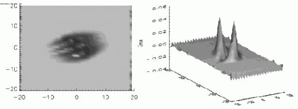
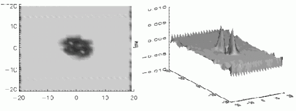
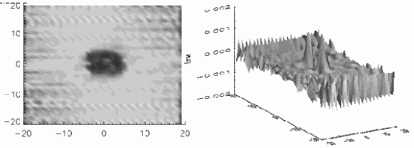
As an example, we illustrate a $200\times 200$ pixel $n=4$ Sérsic model with $r_{e}=10$ pixels. We generate Figure 5a by direct numerical integration with a $\theta=30^{o}$ rotation and we generate Figure 5b using the image generation method in Galphat. The two images appear the same. Differences between the two methods only become obvious when one looks at a relative residual image. Figure 6a, 6b and 6c shows a comparison of the same galaxy (i.e. $n=4$ and $r_{e}=10$) generated using the methods of Galphat to the direct integrated image for three different axis ratios: $q=0.1,0.4,\mbox{and}\ 0.7$, respectively. We zoom in on the central region: $[-2r_{e},2r_{e}]$. The left column in Figure 6a-6c shows the face-on view of the relative residual image and the right column is the view of the relative residual surface, with the magnitude of the residual plotted in the $z$ direction. The maximum relative difference decreases with increasing $q$ and remains much less than 1% except for the extreme case of a concentrated galaxy with $n=4$ and $q=0.1$ (Fig. 6a), which is a very unrealistically small axis ratio for an observed galaxy with an $n$ this large and still only has a 5% maximum error at the centre. The errors in the outer region are negligible and the total flux is still conserved to better than one part in $10^{6}$ in all three cases. Galaxies with smaller Sérsic indices have even smaller errors even when the axis ratio is small; such small axis ratios are more realistic for observed galaxies when the Sérsic index is small. The errors would be further reduced if we generated the images using pixel subsampling.

3.2.3 Computation time for model generation

Table 1: Galphat  model generation time

Image/model	CPU	CPU time (total)	CPU time (interpolation)	CPU time (FFT rotation)
190 by 190	Quad-core AMD Opteron	0.092 sec	0.079 sec	0.013 sec
Sérsic	2613 MHz

The wall clock time for a posterior simulation depends on the model, the image, and the MCMC algorithm. A typical run using the PHS algorithm requires of $\mathcal{O}(10^{5})$ evaluations (see §5.3). Here we provide a CPU time estimate for the generation of a single Sérsic model (Table 1) for an example image with a size of $190\times 190$ pixels. The generation of a single Sérsic model requires 0.092 sec (on a single processor). This is more than an order of magnitude faster than would be required using direct numerical integration over the pixels, and we still preserve high numerical accuracy. Most of the CPU time is spent interpolating the image tables to obtain $I_{jk}$; the FFT rotation is a minor contribution. Since this image is larger than the mean galaxy size in our 2MASS target sample, we conclude that Galphat is both sufficiently fast and sufficiently accurate to be suitable for a large-scale analysis over a large catalogue. (see §5.3 for a discussion of the total MCMC run time).

3.3 The likelihood function and the prior distribution

CCD detectors count photons and this is well-described as a Poisson process. If the model predicts the flux $m_{i}$ for $i$th pixel then the probability that we measure the flux $d_{i}$ for that pixel follows a Poisson distribution, $P(d_{i}|m_{i})=\exp(-m_{i})m_{i}^{d_{i}}/d_{i}!$. Assuming that each pixel is independent, our likelihood function $L(D|\theta)$ is

$$L(D|\theta)=\prod^{N_{pix}}_{i=1}P(d_{i}|m_{i})$$ (23)

where $N_{pix}$ is the total number of pixels and $\theta$ is the parameter set of the Sérsic model. To increase the numerical accuracy, we accumulate the logarithmic value of the probability.

As previously described, the prior distribution of model parameters affects the inference. A preliminary study with non-uniform prior distributions confirms that the posterior maximum and confidence values can be significantly changed for low S/N data that dominate the galaxy population in a flux-limited survey. However, for simplicity, we have used uniform prior distributions for all the parameters for the tests in this paper. Again, the use of an informative prior without careful consideration will almost certainly lead to a biased result. We present a detailed study of prior distributions for inference and model selection for galaxy profiles in our followup paper (Yoon et al., 2010).

3.4 Sampling the posterior probability

It is difficult to ensure that the Markov chain correctly samples from the entire posterior distribution in a high-dimensional parameter space. To combat these difficulties, the BIE uses a variety of algorithms, each with features effective for different problems that impede the efficiency of sampling and convergence. One should characterise the MCMC simulation on representative data using different algorithms before starting any production runs. We find that the PHS algorithm performs best for our problem; it more efficiently samples parameter space and more quickly reaches a steady state compared with the other MCMC algorithms. Here, we will briefly introduce the PHS algorithm (Rigat, 2008).

The PHS algorithm constructs an $n$-rung temperature ladder that powers up or heats the target posterior probability $\pi_{0}$:

$$\pi_{i}=c_{i}\,\pi_{0}^{1/T_{i}}=c_{i}\,e^{(\log\pi_{0})/T_{i}}\quad\mbox{for}\quad n=0,\ldots,n$$ (24)

where $1=T_{0}<T_{1}<\cdots<T_{n}$ and $c_{i}$ is a normalisation constant. The number of chains can be chosen by the user as well as the maximum temperature considering the dimensionality of the model. Each Monte Carlo step has two parts: 1) each chain is updated using a standard Metropolis-Hastings step; and 2) chains at different temperatures may be swapped by one of two algorithms: i) each chain state is updated at fixed temperature or swapped with a chain state at an adjacent temperature following a fixed swapping probability (standard parallel chains); or ii) an exchange is proposed between the cold (fiducial) chain and one of the warmer chains and the remaining chains are updated at fixed temperature. At the end of the run, the fiducial chain with $T_{0}$ samples the posterior distribution.

3.5 Chain convergence

Monte Carlo simulations of the posterior distribution may suffer from two classes of difficulties: 1) the Markov chain is mixing poorly in a particular mode in the posterior distribution, and this leads to a large number of dependent states; and 2) the posterior distribution may have two or more discrete modes with similar posterior probability and the Markov chain can not move between them. The first difficultly is easily diagnosed by observing very low or very high acceptance rates and is addressed by tuning the Metropolis-Hastings transition probability. The second difficulty is addressed by a variety of hybrid MCMC algorithms, implemented in the BIE, designed to move between modes. The parallel chain algorithm, and tempering in general, decreases the contrast of the hills and valleys in the posterior distribution, which allows occasional large excursions between modes.

To test for convergence of the cold chain in the PHS algorithm, i.e. the chain with $T_{0}$, we use a subsampled convergence diagnostic (Giakoumatos et al., 1999) for this single chain. The chain is cleaved and used to compare in-chain and inter-chain variances, similar to the Gelman-Rubin (Gelman & Rubin, 1992) test. The ratio of these two variances should approach unity for a converged steady-state chain. We have tested Galphat over a wide variety of synthetic image data typical of observed galaxies, using the empirically determined transition probability, and have confirmed that our MCMC algorithm samples the posterior with a reasonable acceptance rate of $\geq 25\%$ for good mixing and a swapping rate of $\geq 25\%$ for efficient mode exploration.

4 Simulated galaxy images

To characterise the performance of Galphat, we generated an ensemble of 3000 isolated, synthetic Sérsic galaxy images representative of survey observations. We vary both the S/N from 5 to 100 and $r_{e}$ to probe the extremes of barely resolved galaxies and that of galaxies that extend beyond the image frame. The PSF is a Gaussian with a 2.96 FWHM in pixels, which we convolve with the model images. We use a Poisson noise model and a gain factor of 8.0 [$\mbox{e}^{-}$/ADU]. Both of these choices are motivated by 2MASS images. We describe the details of our choices below.

4.1 Varying S/N

We define the signal-to-noise ratio as the ratio of the flux from the galaxy within the half-light radius to the noise from the sky background and the galaxy within the same area:

$$\mbox{{S/N}}=\frac{\langle\rho\rangle}{\sqrt{\langle\rho\rangle+\langle\rho_{sky}\rangle}}$$ (25)

where $\langle\rho\rangle$ is the total electron count of the galaxy profile within the area $\pi r_{e}^{2}q$ and $\langle\rho_{sky}\rangle$ is the background within the same area.

For each of ${S/N}\in\{5,10,20,50,100\}$, we generate 100 Sérsic model galaxies with a randomly chosen combination of uniformly distributed $r_{e}\in[6,20]$ $n\in[0.7,7.0]$, axis ratio $q\in[0.1,1.0]$, and position angle $\mbox{PA}\in[0^{\circ},90^{\circ}]$. We fix the sky background to 300 [ADU]. Once we choose $r_{e}$ and $q$, we determine the galaxy’s magnitude for the given S/N value and magnitude zero point using equation (25).

4.2 Varying $r_{e}$

The inference of $r_{e}$ is biased if the galaxy is small compared to the PSF. To test this, we generate 100 Sérsic model galaxies for all combinations of ${S/N}\in\{5,10,20,50,100\}$ and $r_{e}\in\{0.5,1.0,2.0,4.0,8.0\}$ (in units of $\frac{1}{2}$ FWHM of the PSF) using the same distributions of $n$, $q$, and PA as in §4.1. We compute the Poisson counting errors and the sky background as in §4.1.

5 GALPHAT performance testing

Parametric surface brightness models invariably result in parameter covariance, and this covariance can be exacerbated by instrumental and selection errors. The Bayesian MCMC approach explicitly incorporates parameter covariance, noise sources and other selection effects including data S/N, PSF convolution and the sizes of the galaxy and the image, to yield a reliable inference, as illustrated in §1.1 and §1.2.

Using the simulated galaxies from §4, we investigate the effect of observational attributes such as the S/N, the galaxy’s $r_{e}$ compared to the PSF FWHM, the image size compared to galaxy’s $r_{e}$, and errors in the assumed PSF FWHM. Although we generated 40,000 converged MCMC states for each image, we do not use the full 40,000 MCMC states to construct the posterior since we want a more conservative estimate of the burn-in period than that diagnosed by the convergence test. As previously described, we use the PHS algorithm (Rigat, 2008) for all of our tests and determine convergence using the subsampled convergence test (Giakoumatos et al., 1999). We tune the width of the Metropolis-Hastings transition distribution to yield, roughly, a 25% acceptance rate and 25% chain swapping rate for each chain. The prior distribution of the galaxy centroid is normal with a mean at the image centre and a $\sigma=$3 pixels. The sky background prior is also normal with a mean of the input sky background and a $\sigma=$0.5 ADU. The prior distributions for the other model parameters have a uniform probability within a finite range.

5.1 Examples of single fits

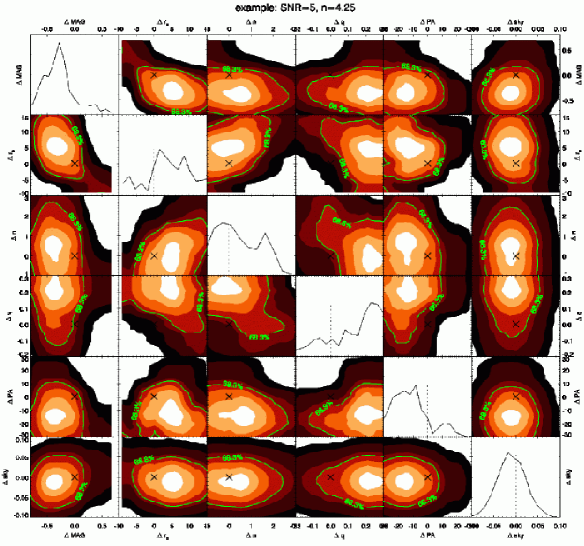
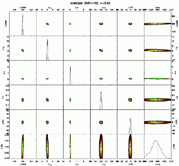
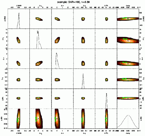
Before we present our results for an ensemble of galaxies, we present the results of Galphat fits to four galaxies. From the simulated galaxy sample, we picked four example galaxies, two that represent elliptical galaxies ($n\approx 4$) and two that represent exponential disc ($n\approx 1$) galaxies. One galaxy of each type has a low S/N of 5 and one has a high S/N of 100.

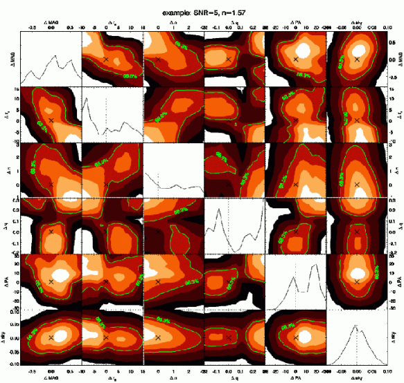
In Figures 7–10 we show the marginalised posteriors of the galaxy magnitude (MAG), the half-light radius ($r_{e}$), the Sérsic index ($n$), the axis ratio ($q$), the position angle (PA), and the sky background (sky). Figures 7 and 8 show the results at low S/N for an exponential disc-like galaxy and an elliptical-like galaxy, respectively, and Figures 9 and 10 show the results at high S/N for an exponential disc-like galaxy and an elliptical-like galaxy, respectively. In each figure, the full marginal distribution for each model parameter residual is shown on the diagonal with the vertical dotted line indicating the zero residual, and the joint marginal distributions of parameter pairs are shown on the off-diagonals with the seven colour contours corresponding to the 10, 30, 50, 68.3 (green solid line), 80, 95 and 99% confidence levels. The locations of the zero residuals are indicated by the $\times$.

When the S/N is small, for both an exponential disc galaxy (see Fig. 7) and for an elliptical galaxy (see Fig. 8), the posteriors are not unimodal and are spread out over a large range in parameter space. Although there is a weak covariance between the magnitude, $r_{e}$, $n$, and the sky background, uncertainties in the parameter inferences are largely dominated by the Poisson random noise present in the image. However, the situation becomes very different at high S/N as shown in Figure 9 for an exponential disc galaxy and in Figure 10 for elliptical galaxy. Note that these figures have the same scale as Fig. 7 and Fig. 8. Now the posterior forms a strong mode close to the true value and the morphology of the posterior is determined by the parameter covariance present in the Sérsic model, which strongly depends on the Sérsic index. There is a stronger parameter covariance among magnitude, $r_{e}$, $n$, and the sky background for the high S/N elliptical galaxy than for the low S/N exponential disc galaxy, which can lead to larger errors when marginalising the posterior distribution.

The Bayesian-based Galphat procedure explicitly incorporates the parameter covariance present in the Sérsic model. Furthermore, it enables us to utilise the entire posterior distribution for a galaxy population to reliably test hypotheses based on that population. This is practically feasible using Galphat, as we will demonstrate in following sections.

Figure 7: Posterior marginals for a galaxy with ${S/N}=5$ and $n=1.57$ (i.e. an exponential-disc galaxy). The full marginal distribution for each model parameter residual is shown on the diagonal with the vertical dotted line indicating the zero point. Joint marginal pairs of parameter residuals are shown on the off-diagonals. The seven colour contours represent the 10, 30, 50, 68.3, 80, 95 and 99% confidence levels and the green solid line is the 68.3% confidence level. The locations of zero points are indicated by $\times$ symbols. Posteriors are not unimodal and are spread over large range in parameter space. Although very weak covariances exist among magnitude, half-light radius ($r_{e}$), Sérsic index ($n$) and sky background, parameter uncertainties are largely dominated by Poisson random noise.

Figure 8: Posterior marginals for a galaxy with ${S/N}=5$ and $n=4.25$ (i.e. an elliptical galaxy). See the caption for Fig. 7. As for the exponential disc galaxy, parameter covariance is not significant and the posteriors spread out owing to noise.

Figure 9: Posterior marginals for a galaxy with ${S/N}=100$ and $n=0.95$ (i.e. an exponential-disc galaxy). See the caption for Fig. 7. Unlike the low S/N case, strong parameter covariances exist among magnitude, $r_{e}$, $n$, and the sky background, and the parameter posteriors are confined in a narrow region close to the true value in parameter space.

Figure 10: Posterior marginals for a galaxy with ${S/N}=100$ and $n=3.80$ (i.e. an elliptical galaxy). See caption for Fig. 7. While parameter posteriors are compact and parameter uncertainty is dominated by parameter covariance, as for the high S/N exponential disc galaxy, there is a stronger parameter covariance among magnitude, $r_{e}$, $n$, and the sky background than for the exponential disc. This leads to inflated errors for individual parameters determined from the marginalised distribution.

5.2 Model covariance and bias

Using the posterior distribution from the converged Markov chain, we illustrate the inherent covariance between parameters by showing joint distributions of selected parameter combinations for the Sérsic model. To emulate a catalogue analysis, we generate an ensemble of galaxies with astronomically representative model parameters for each bin in observational conditions. The dependence on observational conditions are explored in the following several sections.

5.2.1 Effects of galaxy S/N

We characterise the posterior distributions of 500 images for Sérsic models (100 in each S/N bin with a range of structural parameters, see §4.1). Recall that these Sérsic models have 8 free parameters: the centroid coordinates ($x,y$), the magnitude (MAG), the half light radius $r_{e}$, the Sérsic index $n$, the axis ratio $q$, the position angle PA, and the sky background (sky). We use the last 25000 states to characterise the posterior. We constructed an ensemble posterior distribution by pooling the sampled distribution for all the images in each S/N bin.

We show all the marginalised distributions for errors in the magnitude, $r_{e}$, $n$, $q$, PA, and the sky background for each S/N bin in Figures 11, 12, 13, 14 and 15. Hereafter, we use the superscript $i$ to denote the Galphat inferred value. The parameters $r_{e}$ and $q$ are plotted as fractional changes scaled by their input values and the values of the other parameters are the differences from their input values. We quote the sky background error as the fractional percent error, i.e. the fractional change scaled by the input sky background multiplied by 100. Each diagonal subplot is the full marginalised ensemble posterior error distribution of the corresponding parameter with a vertical dotted line indicating the location of the input value. Each off-diagonal subplot is the joint distribution of ensemble error posteriors for the corresponding parameter pair. The seven contour levels are the 10, 30, 50, 68.3, 80, 95 and 99% confidence levels, and the green solid line marks the 68.3% confidence level, corresponding to a “one-sigma” normal confidence. The black crosses indicate the locations of the input values.

Figure 11: Posterior error distributions for the ensemble of galaxies with ${S/N}=5$. The full marginal error distribution for each model parameter is shown on the diagonal. Joint marginal pairs of parameters are shown on the off-diagonals. Galphat inferred parameters $r_{e}^{i}$ and $q^{i}$ are scaled by their input values and the other parameters are differences from their input values. The fractional sky background errors are percentages. The seven colour contours represent 10, 30, 50, 68.3, 80, 95 and 99% confidence levels and the green solid line is the 68.3% confidence level. The locations of the input values are indicated by vertical dotted lines for the diagonal and $\times$ symbols for the off-diagonals. The values of magnitude, $r_{e}$, $n$ and sky background are strongly correlated. Although the constraints are tighter with increasing galaxy S/N, the strength of the parameter covariance increases with increasing galaxy S/N (see Figs. 12–15).

Figure 12: Ensemble parameter error posteriors for galaxies with S/N$=10$. See caption for Fig. 11.

Figure 13: Ensemble error parameter posteriors for galaxies with S/N$=20$. See caption for Fig. 11.

Figure 14: Ensemble error parameter posteriors for galaxies with S/N$=50$. See caption for Fig. 11.

Figure 15: Ensemble error parameter posteriors for galaxies with S/N$=100$. See caption for Fig. 11.

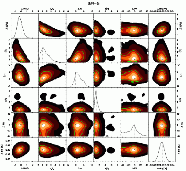
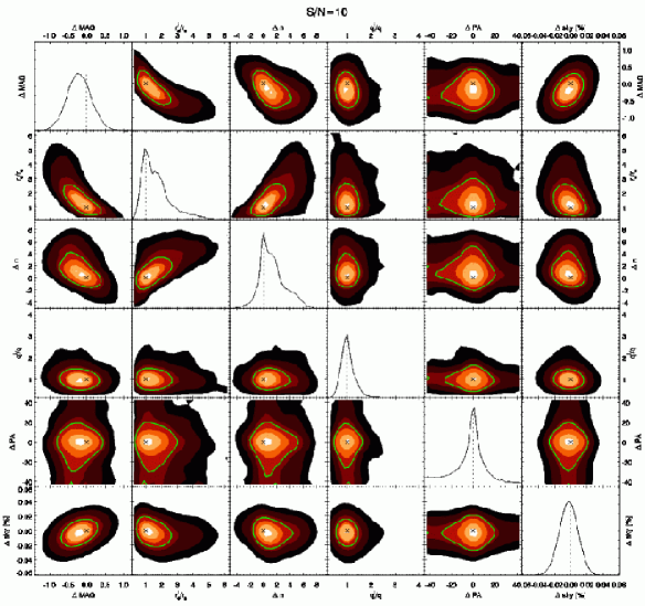
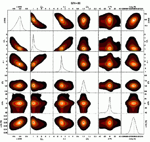
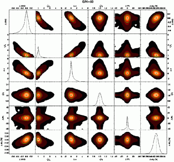
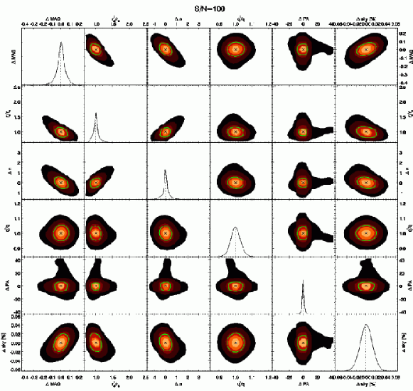
Here, we use galaxies with $6<r_{e}<20$ pixels, larger than the PSF that has a HWHM of 1.48 pixels to reduce the effects of resolution (the posterior distributions of small galaxies are described in §5.2.3). For this sample, $q$ and PA are not covariate with the other parameters. However, the values of the magnitude, $r_{e}$, $n$, and the sky background are obviously covariate, and the covariance becomes stronger with increasing S/N. The origin of this covariance is straightforward to understand. For a given surface brightness profile, a magnitude underestimate (i.e. a luminosity overestimate) results in an overestimate of $r_{e}$ to better match the observed brightness distribution. Since the Sérsic model parameters $r_{e}$ and $n$ have a positive correlation (e.g. Trujillo et al., 2001), $n$ is also overestimated. Similarly, the sky background is underestimated to help compensate for the underestimated magnitude. This argument also holds exactly in the opposite direction for an overestimated magnitude. The shape of the joint posterior distributions in Figures 11–15 show that the strength of the parameter covariance depends on galaxy S/N (and Sérsic index $n$ as will show in §5.2.2).

In concert with our intuition, the confidence regions for $q$ and PA shrink with increasing galaxy S/N. For example, the asymmetric heavy-tailed residual posterior distribution in $\Delta PA$ clearly seen in Figure 11 becomes symmetric as S/N increases (Figs. 12–15). This tail has its origin in the ambiguity of $PA$ for $q\approx 1$.

The covariance of magnitude, $r_{e}$, $n$ and sky background also changes with galaxy S/N. For low S/N (S/N$=5$, Figure 11), pairs of these parameters exhibit a clear covariance; the sky background is strongly covariant only with the magnitude. Also notice that the marginalised distributions of the errors in the magnitude and $n$, and of fractional errors in $r_{e}$ are not normal as is conventionally assumed and that the 68.3% confidence region is not elliptical. This non-normal behaviour results from the lack of information at low S/N to constrain one or more of the covariate parameters.

As the S/N increases, the covariance of the magnitude, $r_{e}$, $n$ and the sky background increases while the confidence regions decrease (see Figures 12–15) and the asymmetry of the marginalised posterior distributions vanishes. The posterior distribution is dominated by the likelihood function, which is sharply peaked and approaching its asymptotic form. In addition, the strength of the correlation depends on $n$ owing to the strong correlation of $n$ with the sky background. This can be seen in the joint posteriors of $n$ and the sky background in Figures 13–15 where the confidence level contours appear to be mixture of different covariance ellipses from groups of galaxies with different $n$, as will be shown in the next section.

5.2.2 Effects of Sérsic index $n$

To investigate trends with the Sérsic index $n$, we selected four model parameters to study in depth, magnitude, $r_{e}$, $n$ and sky background, for ${S/N}=5,20,100$. We divide the samples in each S/N bin into two groups: $n>2.0$ and $n\leq 2.0$. We show the marginalised posterior error distributions for each group in Figures 16–18. The contours and curves for the samples with $n\leq 2.0$ and $n>2.0$ are shown by the blue and red colours, respectively. The contour levels for each group corresponds to the 68.3, 95.4, and 99.7% confidence levels. The black crosses are the locations of the input values and the grey contours and grey curves show the total sample as in Figures 11, 13, 15.

Figure 16: Posterior error distribution for magnitude, $r_{e}$, $n$ and sky background with ${S/N}=5$ from Figure 11 separated by $n>2.0$ (red) and $n\leq 2.0$ (blue). Confidence levels are 68.3, 95.4 and 99.7% and the input value is marked by a $\times$ and a vertical dotted line for joint and marginal distribution respectively. Grey contours and curves represent the total sample. The parameter covariance is strong when $n$ is large.

Figure 17: Posterior error distribution for selected parameters with S/N$=20$ from Fig. 13. See caption for Fig. 16.

Figure 18: Posterior error distribution for selected parameters with S/N$=100$ from Fig. 15. See caption for Fig. 16.

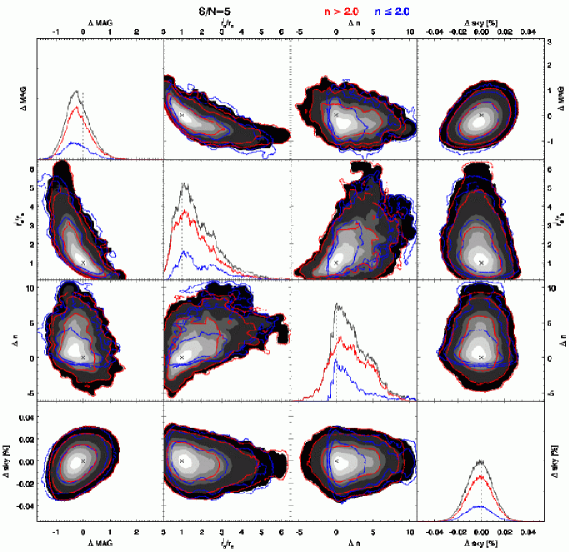
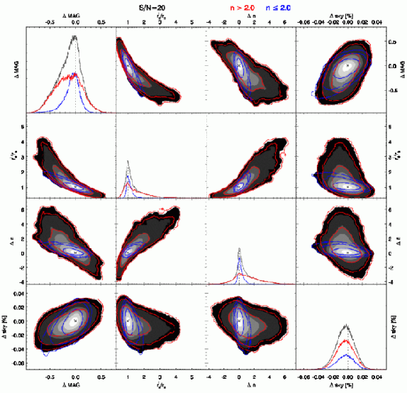
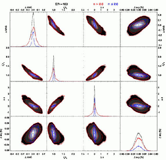
For S/N$=5$ (Fig. 16), the marginalised error posterior for $n\leq 2.0$ has a sharp truncation on the left hand side, owing to the prior distribution boundaries of 0.5 and 11.99 on $n$. Otherwise, the posterior error distributions of these two groups are similar. As expected for low S/N, the errors are dominated by random statistical errors and parameter covariance is not significant. However, for higher S/N (see Figs. 17 and 18), the differences between low and high values of $n$ are significant. When the S/N$\geq 10$, the confidence regions for $n>2.0$ galaxies (red) are larger than for those with $n\leq 2.0$ (blue). In part this is a consequence of the degeneracy between the sky background and the extended profile for larger values of $n$, which makes the morphological parameters for small $n$ galaxies better constrained. One can see the larger covariance for $n>2.0$ in the joint posterior error distributions shown in Figures 17 and 18.

Moreover, covariance with the sky background significantly affects the inference of the magnitude and $r_{e}$. For example, when ${S/N}=100$, a $\pm 0.04$% variation in the sky background estimate may lead to an uncertainty in the magnitude of up to $\pm 0.2$ for elliptical galaxies, i.e. those with $n>2.0$. Conversely, ignoring the sky background uncertainty can induce a significant bias in the other parameters that would be difficult to assess only using the best-fit parameters from a simple $\chi^{2}$ minimisation. Our approach incorporates the parameter covariance and random statistical uncertainty in any subsequent inference. Finally, we note that the parameter distributions of both large and small $n$ galaxies is weakly biased at worst. This demonstrates that the Galphat-inferred posterior maximum reliably recovers the true input parameters. We expect that careful attention to prior distributions could reduce the bias for lower values of S/N as well.

5.2.3 Effects of galaxy $r_{e}$

The intrinsic shapes of small galaxies are obscured by the PSF. Although any pixelisation method induces some bias for any sized galaxy, if $r_{e}$ is comparable to or smaller than the PSF width, the axis ratio $q$ will be be unrecoverable since the central pixels will contain most of the flux. Moreover, numerical techniques without explicit error control when computing $I(x,y)$ (see eq. 9) may fail to produce an accurate theoretical prediction for the model flux in the central pixels. Galphat naturally addresses both problems. Firstly, the Bayesian inference produces an estimate conditioned on the true value of the PSF and, therefore, will produce a posterior distribution consistent with all the possible models that yield the observed profile after convolution with the PSF. Secondly, the Galphat model images are generated by interpolating a numerically integrated table that is accurate over the entire area of the galaxy with a numerical error tolerance set by the user. In particular, both the inner and outer profiles are well-resolved because the tabulated grids are independent of scale. In other words, it is not possible for Galphat to produce a poor estimate of the central pixel values for any value of $r_{e}$.

Even when accurately determined, the true value of $q$ affects the other structural parameters because a small galaxy with a small $q$ takes up fewer image pixels. Similar to §5.2.2, we investigate these effects in Figures 19–22 by dividing the galaxy sample into two groups: $q>0.3$ (red) and $q\leq 0.3$ (blue), and by examining the posterior error distributions of magnitude, $n$, $r_{e}$, and $q$. We also select two bins in size: $r_{e}=0.5$ times the HWHM of the PSF and $r_{e}=8.0$ times the HWHM of the PSF, for two different values of S/N: 20 and 100.

Figures 19 and 20 show the posterior error distributions for galaxies with $r_{e}=0.5$ times the PSF HWHM for a S/N of 20 and 100, respectively. The three contours on the background grey contours, which indicate the total sample, denote the 68.3, 95.4 and 99.7% confidence levels for galaxies with $q>0.3$ (red) and $q\leq 0.3$ (blue). Since the PSF dilutes any evidence of the intrinsic shape inside the PSF FWHM, the posterior error distributions of $r_{e}$ and $q$ have significant probability density at larger values than the input values. Moreover, the magnitude is covariant with $r_{e}$ and $q$. As a consequence, the posterior distribution of magnitude has significant probability at values smaller than the input value. Similarly, the bias in the Sérsic index $n$ is exacerbated by its covariance with $r_{e}$.

In Figure 19, the posterior error distribution for $r_{e}$ has a tail to large $r_{e}$ for both $q>0.3$ and $q\leq 0.3$. As a result, the maximum of the posterior distribution in $n$ is also similarly biased to large $n$ for both groups. The bias in the two groups for $q$, however, is dramatically different: for $q\leq 0.3$ (blue) the distribution is approximately uniform over a large range, while for $q>0.3$ (red) the distribution has a mode centred near 1. This is an artifact of the PSF convolution; the PSF naturally makes the galaxy appear rounder. Therefore, the bias in $q$ for rounder galaxies is modest but the bias for flat, intrinsically edge-on galaxies is large.

The residual magnitude distribution for the entire sample (grey) is slightly negatively biased owing to the excess posterior probability of $r_{e}$ at larger parameter values than the true value. The bias differences in $q$ for the two groups leads to a bias difference in magnitude: the bias for $q\leq 0.3$ (blue) is larger than the bias for $q>0.3$ (red). As described above, the posterior distribution for $q$ are biased upwards as $q$ decreases. On the other hand, because $q$ is poorly constrained, the luminosity can be adjusted in a variety of ways to achieve the same surface brightness for a given $r_{e}$ by making both $q$ and the luminosity either large or small (see eq. 8). This results in both a large spread in magnitude as well as a magnitude underestimate owing to a luminosity that is overestimated to compensate for the upward bias in the posterior distribution of $q$.

Figure 19: Posterior error distributions for magnitude, scaled $r_{e}$, scaled $q$ and residual $n$ with ${S/N}=20$ and $r_{e}=0.5\ \mbox{PSF HWHM}$, separating samples with $q>0.3$ (red) and $q\leq 0.3$ (blue). Input values are shown by a $\times$. Contours are 68.3, 95.4 and 99.7% confidence levels. The grey scale contours and curves represent the total sample. When a galaxy is close to edge-one (i.e. $q<0.3$) and smaller than the PSF, the marginalised posterior of $q$ is almost flat and the posterior maximum of magnitude is negatively biased (i.e. the luminosity is overestimated).

Figure 20: Posterior error distributions for selected parameters with $r_{e}=0.5\ \mbox{PSF HWHM}$ and S/N=$100$. See caption for Fig. 19.

Figure 21: Posterior residual distributions for selected parameters with $r_{e}=8.0\ \mbox{PSF HWHM}$ and S/N=$20$. See caption for Fig. 19.

Figure 22: Posterior error distributions for selected parameters with $r_{e}=8.0\ \mbox{ PSF HWHM}$ and S/N=$100$. See caption for Fig. 19.

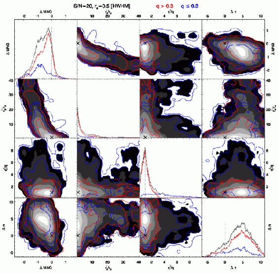
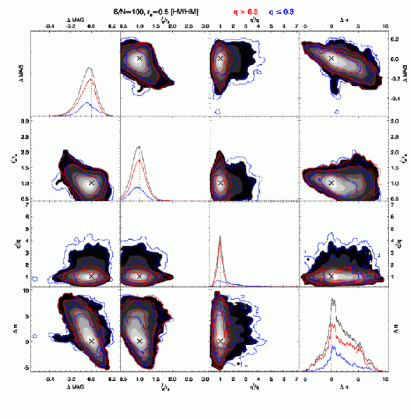
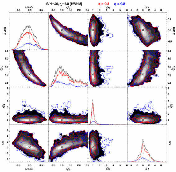
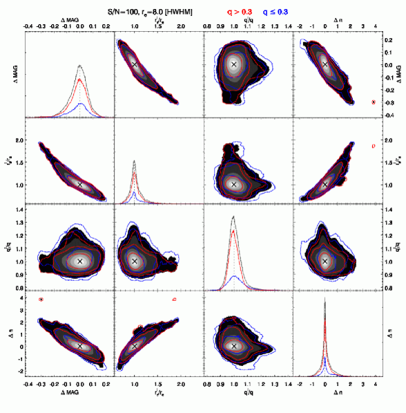
Figure 20 shows the posterior error distributions for ${S/N}=100$. As anticipated, the posterior distributions are better confined in parameter space and the biases of the posterior maxima are significantly reduced, e.g. the error posterior for $n$ has a mode at 0. The posterior maxima for $q>0.3$ galaxies (red) show no strong biases. The posterior error distribution for $q$ when $q\leq 0.3$ (blue) reveals an extended tail and, in contrast to Figure 19 for low S/N, it has a mode below 1.

As $r_{e}$ increases beyond the PSF size, we expect these biases to decrease. Figures 21 and 22, which show the results when $r_{e}=8.0\ \mbox{HWHM}$ of the PSF for a S/N of 20 and 100, respectively, confirms this expectation. The bias of the posterior maximum is modest and the differences between the $q>0.3$ and $q\leq 0.3$ groups disappear. Also, for fixed $r_{e}$, the confidence regions decrease with increasing S/N, as expected.

5.2.4 Effects of image size

We have seen that Sérsic model parameters, such as the magnitude, $n$, and $r_{e}$ are covariant with the sky background. Therefore, an inaccurate sky background determination may bias the inferred galaxy structural parameters. To circumvent this, researchers have measured the sky background independently from their model fits. If the sky background measurement is not more precise than the model fit itself, this procedure has two disadvantages: 1) because of the covariance, the subsequent parameter posterior distribution will be biased; 2) characterisation of the covariance will no longer be part of the posterior distribution.

The Bayesian MCMC approach implemented by Galphat enables us to take all the parameter covariances into account in our galaxy modelling. In particular, we may characterise the influence of parameters such as the sky background. In this section, we explore the influence of the blank-sky fraction in the image. Assume that one must analyse a particular source on a large image. How much of the frame should one keep for one’s parameter inference? Retaining a large fraction of blank sky area is better to accurately determine the sky background. However, a larger fraction of blank sky implies a larger image size and more computation time. Of course, truly blank sky is rare in Nature. Nonetheless, an understanding of the trade-off between an accurate sky background determination and a fast model image generation is necessary to design an efficient analysis. We test the dependence on image size by generating 10 simulated galaxies with ${S/N}=50$, $r_{e}=10$ pixels, $n=4$, $q=1$, and a 500 [ADU] Poisson sky background and model them using different size image regions specified by 4, 8, 12, 16 and 20 times $r_{e}$. We add 30,000 converged MCMC states from each galaxy to obtain the posterior error distribution.

Figure 23: Posterior error distributions of the sky background for images with different sizes. Ten galaxies with the same Sérsic model parameters but different random noise, are modelled with different size image regions, from 4 to 20 times the input $r_{e}$. The galaxies have S/N$=50$, $n=4$, $r_{e}=10$, $q=1$ and a Poisson distributed sky background with 500 ADU. Within each bin, an ensemble of parameter error posterior from the 10 galaxies is shown with posterior maximum (cross symbol), 68.3% (grey box), 95.4% (red box) and 99.7% (blue box) confidence levels. Minimum and maximum data values are indicated by the error bars. Although the sky background posterior is nearly symmetric regardless of the blank sky fraction in the image, the posterior maximum becomes slightly biased downwards with increasing confidence intervals as the blank sky fraction decreases.

Figure 24: Error posteriors of magnitude, $r_{e}$, $n$ and sky background when the image region is $4r_{e}$. The green line highlights the 68.3% confidence level. Note that a $0.1\%$ bias in the sky background posterior maximum leads to biases in the other parameters, e.g. -0.3 in magnitude, and the inference for $r_{e}$ is very weak.

Figure 25: Error posteriors of magnitude, $r_{e}$, $n$ and sky background when the image size is $20r_{e}$. See caption for Fig. 24. Note that the parameter inference becomes more reliable with increasing image size.

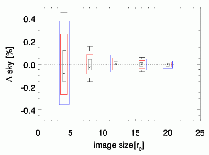
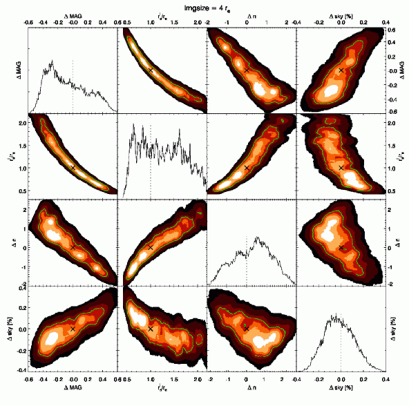
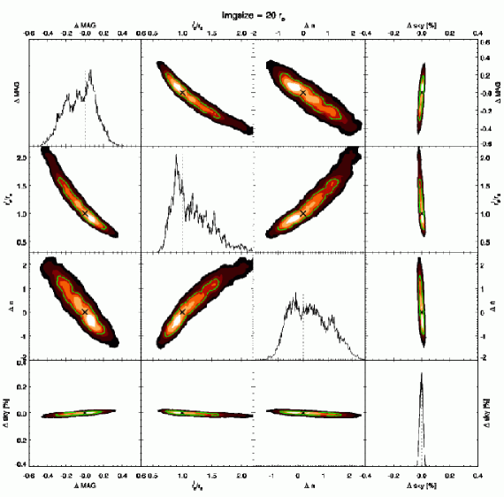
Figure 23 shows the marginalised error posterior distributions for the sky background of the Sérsic model as a function of image size. The cross indicates the posterior maximum and the 68.3, 95.4 and 99.7% confidence levels are indicated by the grey, red and, blue boxes, respectively. The minimum and maximum data values are indicated by the error bars. Although the Galphat inference of the sky background has a symmetric posterior error distribution around zero, regardless of the blank sky fraction in the image, the posterior maximum is below the true sky value as the blank sky fraction decreases. Since the galaxy surface brightness model, i.e. a Sérsic profile, is degenerate with the sky background in the outer regions, a small image containing a relatively large galaxy may introduce a bias in the posterior distribution of the sky background and hence also affects the inference of the other parameters. In other words, owing to the Sérsic model surface brightness and sky background degeneracy, either increasing the galaxy luminosity and decreasing the sky background or decreasing the galaxy luminosity and increasing the sky background can match the background level of the image. However, this flexibility in a Sérsic profile to produce the sky background allows a galaxy to include part of the sky background flux and thus the sky background posterior tends to be biased downwards as we show in Figure 24. This sky background bias that stems from not enough information about the blank sky in the image becomes more significant with increasing $n$. The Galphat inference of the sky background for this particular case of $n=4$ is not biased unless the image size is smaller than $12r_{e}$ and the bias in the sky background posterior maximum is very small, only $0.1\%$, even when the image only extends to $2r_{e}$.

However, it is remarkable that this tiny sky background bias leads to significant biases in the inferences of the other parameters, i.e. the magnitude, $r_{e}$, and $n$, as shown in Figure 24 where we plot the error posteriors of the magnitude, $r_{e}$, $n$, and the sky background for a galaxy with $n=4$ and an image size of $4r_{e}$. In addition to the strong parameter covariances already illustrated in §5.2.1 and §5.2.2, notice that the posterior maximum of the magnitude is biased low by 0.3 owing to the very small ($0.1\%$) bias in the sky background posterior maximum and that the posterior distribution of $r_{e}$ is very broad. If the image size increases, these biases and weak inferences become less significant as shown in Figure 25, which shows the case when the image size is $20r_{e}$.

Even this simple test using a small number of galaxies reconfirms the importance of an accurate sky background. In addition, it illustrates that an accurate characterisation of measurement uncertainties is essential to limiting bias. Therefore, rather than fixing or subtracting a sky background determined by a independent measurement, one must model the galaxy image including the sky background and characterise the full posterior distribution of the model parameters. Although Galphat can handle the interactions of random uncertainties and parameter covariance over a wide range of images sizes, the bias is reduced with an image size of at least $10r_{e}$ for a galaxy with $n=4$.

5.2.5 Effects of assumed PSF errors

Errors in the assumed PSF will lead to errors in the Galphat inferred parameters. We characterise PSF errors by the difference in PSF FWHMs:

$$\Delta\mbox{FWHM}=\frac{\mbox{FWHM}_{assumed}-\mbox{FWHM}_{true}}{\mbox{FWHM}_{true}}.$$

We investigate Galphat-sampled posterior error distributions for Sérsic models using a PSF with $\Delta\mbox{FWHM}=-15\%,-5\%,5\%,15\%$. From the sample of simulated galaxy images in §4.2, which were convolved with a 2MASS-motivated 2.96 FWHM pixel PSF, we select galaxies with a ${S/N}=100$ and in four $r_{e}$ bins of size 1, 2, 4 and 8 times the PSF HWHM of 1.48 pixels.

Figure 26: The posterior maximum errors of $r_{e}$ and $n$ for errors in the assumed PSF widths with $\Delta\mbox{FWHM}=15\%,5\%,-5\%,-15\%$ as labelled. The error bars show the $p=0.5$ confidence interval. The biases in the posterior maximum become smaller with increasing galaxy size.

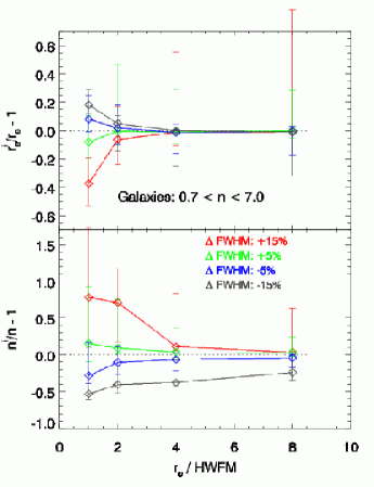
We show the results in Figure 26 where we plot the posterior maximum of relative error in $r_{e}$ and $n$ with the error bar indicating the $50\%$ confidence interval for the four different $\Delta\mbox{FWHM}$s. If the PSF width were overestimated, we would expect that the inferred galaxy size would be smaller than its true size and that the inferred profile would be more concentrated, i.e. a larger $n$ than the intrinsic value, and vice versa. Figure 26 confirms these expectations. Also as expected, the bias of the posterior maximum is less if the galaxy size becomes larger than the PSF FWHM. The bias of the $r_{e}$ posterior maximum is larger when the PSF is overestimated than when it is underestimated as previously observed by MacArthur et al. (2003). Moreover, notice that there is a systematic offset of the ensemble posterior maximum of $n$ even if the galaxy’s $r_{e}$ is large, indicating that the bias of the $n$ posterior maximum owing to errors in the assumed PSF FWHM also depends on $n$ itself.

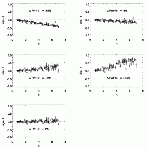
We characterise the $n$ dependent bias by investigating the posterior error distribution of $n$ for the galaxies with $r_{e}=8\ \mbox{HWHM}$ of the true PSF. Figure 27 plots the relative errors in the median values of the Galphat posterior samples ($n^{i}$) of $n$ as $\Delta n=\frac{n^{i}-n}{n}$ for each galaxy in each of the PSF error samples: $\Delta\mbox{FWHM}=-15\%,-5\%,0\%+5\%,15\%$. The median values of $n^{i}$ are biased and this bias becomes large as $n$ increases. When the assumed PSF FWHM is overestimated, $n$ is overestimated with increasing $n$ since the larger PSF artificially extends the profile and conversely when the assumed PSF FWHM is underestimated, $n$ is underestimated with increasing $n$ since the smaller PSF artificially contracts the profile. The biases and uncertainties in $n^{i}$ for PSF FWHM overestimation are larger than for PSF FWHM underestimation. For example, the inferred value $n^{i}$ for an elliptical galaxy with $n=4$ will be smaller than the true value by 20% if the assumed PSF FWHM is smaller than the correct PSF by 15%, but it will be larger by 30% with considerable scatter if the assumed PSF FWHM is larger than the correct PSF by 15%. If the correct PSF is used then the inference of $n$ is unbiased but the scatter still increases with $n$.

Figure 27: Systematic bias in the inferred galaxy Sérsic index $n$ owing to assumed PSF width errors based on the posterior error distributions for 100 galaxies with ${S/N}=100$ and $r_{e}=8\ \mbox{HWHM}$ of the PSF using 4 different assumed PSF FWHM errors with $\delta\mbox{HWHM}=-15\%,-5\%,+5\%,+15\%$. Each diamond with error bar is the median and 50% confidence range for the relative difference between the inferred value and the input value. The bottom left panel shows results for the correct PSF.

5.3 Run time

Table 2: Galphat  wall clock time

Image/model	samples	CPU	Processors	wall clock time	MCMC algorithm
$226\times 226$	40,000	Quad-core AMD Opteron	8	$1.5$ hr	hierarchical tempering parallel chain
Sérsic		2613 MHz
$100\times 100$	40,000	Quad-core AMD Opteron	8	$0.4$ hr	hierarchical tempering parallel chain
Sérsic		2613 MHz

The Galphat run time depends on the MCMC algorithm, the complexity of model, the size of model image, the desired number of converged samples, and the number of model components. Although it is difficult to characterise the Galphat run time for each dependency, we find that the dependence on the number of converged MCMC states and on the size of the image, i.e. number of pixels, are approximately linear. However, the dependence on the MCMC algorithm (i.e. the temperature ladder and the number of chains, which depends on the parameter dimensionality) and the model complexity (i.e. the number of dimensions, the number of model components, and the parameter covariance in the chosen model family) are nonlinear. Therefore, it requires some experimentation to find the best strategy for each application. By cross-checking with different MCMC algorithms e.g. simulated tempering (Neal, 1996) or differential evolution (Braak, 2006) with tempering, for a subset of galaxy samples, we were able to tune the parameters for the PHS algorithm used in our study.

Table 2 shows an example of Galphat run time for two galaxy images: one is typical of a 2MASS galaxy image and the other is a relatively large image, which we choose intentionally to demonstrate Galphat’s feasibility in a marginal case as could occur for a 2MASS galaxy image, since we plan to analyse 2MASS galaxies in the future. Table 2 lists the total wall clock times of two example simulations for 40,000 converged states in $226\times 226$ and $100\times 100$ pixel images for the Sérsic model. The number of chains used for Sérsic modelling is 8. The BIE assigns one processor per chain. The run time is the total time for obtaining the 40,000 converged samples using the PHS MCMC algorithm. The necessary number of converged samples depends on the application. Tests are carried out using the University of Massachusetts Astronomy department HPC cluster.

For a Sérsic model, 40,000 converged samples for one galaxy with a typical image size of $100\times 100$ can be obtained within 25 minutes of wall clock time using 8 processors. This of course means it would take 3.2 hours on a single quad core processor or 0.5 days on a single core processor. This may seem computationally impractical but multi-core processors and multi-processor machines are becoming the norm and of course processor speeds and machine sizes are increasing all the time. For example, even now, each of our cluster nodes had 16 processors. Employing 32 nodes of our cluster for one day would yield the posterior distributions of about 3000 galaxies. This means that 10,000 2MASS galaxies can be analysed using a single Sérsic model in less than 4 days using 32 of our 16 core nodes, demonstrating the current feasibility of this approach.

6 Summary

We introduce Galphat, a Bayesian galaxy morphology analysis package, designed to efficiently and reliably generate the probability distribution of galaxy surface brightness model parameters from an image. We emphasise that the morphological analysis is a stepping stone in a larger chain of inference on theories of galaxy formation and evolution. Therefore, we believe that it is productive to consider the determination of galaxy morphology in the context of hypothesis testing and model comparison, and this demands the full posterior probability distributions for each galaxy in the ensemble.

In this section, we recap the history of morphological analyses, summarise the technical improvements offered by Galphat, list major findings from our performance tests, and briefly describe our future work.

6.1 Recap

Our approach offers a number of significant advantages for estimating surface brightness profile parameters. First, the topology of the likelihood function is almost certain to be multimodal in the high-dimensional space. Downhill optimisation techniques demand precise prior information that is not generally available. In addition, one should have a way of assessing the significance of this global extremum with respect to nearby local and possibly unanticipated modes. Using the various tempering algorithms available in the BIE, our tests have demonstrated that we can achieve a steady-state distribution and the simulated posterior will include any possible multiple modes supported by the prior distribution. Given the posterior distribution, we may then precisely estimate the confidence levels. Secondly, the model will often have correlated parameters. As illustrated in §1.1, any hypothesis testing that uses the ensemble of best-fit parameters will be affected by these correlations. The full posterior distributions from Galphat identify these correlations and incorporate them in subsequent inferences.

We can use posterior simulations over ensembles of images to test the significance of cluster and field environments on galaxies as evidenced in their photometric parameters. A more elaborate model might include angular harmonics of the light distribution (e.g. galactic bars and spiral arms); we could use Bayes factors to assess the support in the data for various harmonics. We could do this for an entire set of galaxy images in multiple bands simultaneously. This is much more natural and likely to be more powerful than the standard practice of cataloguing parameters and attempting to look for correlations in scatter plots.

Furthermore, the adoption of specific functional families that resemble galaxy profiles, e.g. Sérsic, may not provide the best discrimination in attempting to interpret the correlation between derived parameters and hypotheses. Our extensive study of Sérsic profiles undertaken for this paper convinces us that the strong inter-parameter covariances weaken the inference. This suggests that families of orthogonal functions conditioned to match the outer galaxy profile might be a more productive choice (e.g. Spergel, 2010). A complete set of orthogonal functions might be straightforwardly transformed to match a fiducial profile, opening up a wide range of possible applications for characterising galaxy properties. With carefully chosen prior distributions, we can use Bayes factors to test the significance of multiple component models and models with different functional forms. This analysis can straightforwardly answer questions such as: is the standard model (Sérsic and exponential disc profiles) preferred to all competing models (models with cores, dark-matter profiles) and vice versa? Is there a particular alternative model that is supported more significantly by the data? We will explore some of these possibilities in our follow-up paper (Yoon et al., 2010).

6.2 Galphat features

Galphat is built on the Bayesian Inference Engine, BIE (Weinberg & Moss, 2010), an object-oriented optimised parallel platform for Bayesian computation. The BIE implements a variety of algorithms and tools that can be chosen at run time to match the problem at hand. For example, in the tests presented here, we have found that the PHS algorithm (Rigat, 2008) provides the fastest convergence while efficiently exploring the parameter space. Other algorithms may excel for different model families or for those with additional components. In addition, the BIE enables collaboration: new algorithms developed for the BIE become available for the community.

These methods require more frequent likelihood evaluations than competing approaches, so optimisation is essential. Galphat incorporates the following key features: 1) pre-computed images using a scale-free relocatable interpolation scheme with strong error control; subsequent image generation accurately represents the surface brightness integrated over every pixel and is very fast; and 2) a Fourier shift-theorem-based rotation algorithm that is both accurate and much faster than the often-used interpolation methods. Although we explore Sérsic models in this paper, Galphat can be applied to a wide variety of parametric families, limited ultimately by the physical memory available to store the lookup tables. The likelihood calculation time for a Sérsic model is less than 0.1 sec for an image size of $190\times 190$ pixels.

6.3 GALPHAT performance on Sérsic profiles: parameter covariance and bias

A summary of our major findings are as follows:

1. Galaxy S/N. Computation of the posterior distribution enables assessment of parameter covariance that includes the full error model. For the Sérsic model, the magnitude, $r_{e}$, $n$ and the sky background are strongly correlated, and the strength of the correlation increases with S/N. The covariance of the sky background with the other model parameters, i.e. the magnitude, $r_{e}$, and $n$, shows that a reliable inference requires an accurate characterisation of the background noise. We fully expect that analogous trends will obtain for most parametric models.

2. Sérsic index $n$. The parameter correlation increases with increasing Sérsic index $n$. As a consequence, the confidence intervals for magnitude, $r_{e}$, and $n$ for galaxies with $n>2.0$ are roughly three times larger than those for $n\leq 2.0$. However, the marginalised error posteriors of the sky background for these two groups do not have significantly different widths. Again, this underscores the need for the entire posterior distribution for subsequent inferences based on morphological quantities.

3. Galaxy $r_{e}$. If $r_{e}$ is smaller than the PSF HWHM, most parameters are poorly constrained and the posterior maximum is biased. For example, the posterior distribution of $r_{e}$ has a significant probability at larger $r_{e}$ than the true value for a non-informative prior. Similarly, the inference of axis ratio $q$ will be positively biased for intrinsically small $q$. Both biases lead to an overestimate of the total flux. As a galaxy’s $r_{e}$ becomes larger compared with the PSF HWHM, this bias decreases. Also, the bias decreases with increasing S/N even if $r_{e}$ is smaller than the PSF HWHM.

4. Image size. We find that the inferred value for the sky background is nearly symmetric about the true value even for an $n=4$ Sérsic profile with an image size of $8r_{e}$. The background bias disappears and the uncertainty drops dramatically for image sizes larger than approximately $10r_{e}$. The covariance of sky background with galaxy surface brightness parameters motivates including the sky background in the overall model to ensure that the correlations are represented in the posterior probability distribution.

5. PSF variation. Errors in the assumed PSF width introduce a bias in the posterior distributions of galaxy size $r_{e}$ and Sérsic index $n$. If the PSF FWHM is overestimated, the galaxy’s $r_{e}$ is underestimated and its $n$ is overestimated, and vice versa. The bias in the inferred value of $n$ increases with $n$. The bias increase is larger if the PSF width is overestimated rather than underestimated.

6. Run time. Galphat’s run time depends on the Monte Carlo algorithm, the desired size of the converged sample, the image size, and the model complexity (i.e. the number of model parameters and the parameter covariance) and the computational complexity. Based on extensive experiments, we found that the PHS MCMC algorithm efficiently sampled the posterior for most of our Sérsic model tests. The typical wall clock times for generating 40,000 converged posterior MCMC samples of galaxies with image sizes of $226\times 226$ and $100\times 100$ pixels, using Sérsic model are about 1.5 (with 8 CPUs) and 0.4 (with 8 CPUs) hours, respectively, using 2GHz AMD quad-core Opteron processors.

   Although the optimised algorithms used in Galphat significantly improves the likelihood computation time, it is still much slower than other conventional galaxy image decomposition algorithms. However, the existence of posterior probability distributions for an ensemble of galaxies enables reliable inferences for models of galaxy formation and evolution, and we feel that this more than compensates for the increased computational overhead. Moreover, the overhead will continue to decrease with the increasing availability and performance of HPC-class facilities.

6.4 Future work

We have investigated a two-component bulge and disc model composed of Sérsic bulge with varying $n$ and exponential disc component with $n=1$ with mutual independent prior distributions. This naive model exhibits strong correlations between multiple dimensions in parameter space, and these occasionally lead to poorly mixing Markov chains. From this preliminary study, we are convinced that a thoughtful prior distribution that removes astronomically unnatural regions of parameter space is required for production work. Yoon et al. (2010) investigate Galphat two-component bulge and disc model fits and introduce an informative prior based on typical 2MASS survey data. Using both bulge and disc two-component and single Sérsic models, we study the sensitivity of prior-distribution choice on the inference of galaxy parameters, demonstrate the practicality of model selection, the preference of a two-component bulge and disc model versus a single Sérsicmodel, using Bayes factor analyses, and illustrate the application of posterior distributions from an ensemble of galaxy images to large-scale inference problems.

In addition, we are currently using Galphat to study the morphology of a $K_{s}$-band magnitude limited sample of 2000 2MASS galaxies in the SDSS footprint, and will accurately characterise the luminosity functions of each component, i.e. the bulge and the disc, separately, and investigate any intrinsic correlations between the model parameters and any correlations with external galaxy properties such as star formation rate and environment in a forthcoming paper. We hope that Galphat will become a well used tool to aid in our understanding of galaxy properties in the near future.

References

- Abadi et al. (2003a) Abadi et al. M. G., 2003a, ApJ, 591, 499
- Abadi et al. (2003b) Abadi et al. M. G., 2003b, ApJ, 597, 21
- Allen et al. (2006) Allen et al. P. D., 2006, MNRAS, 371, 2
- Andreon et al. (2008) Andreon et al. S., 2008, MNRAS, 383, 102
- Bellman (1961) Bellman R., 1961, Adaptive Control Processes: A Guided Tour. Princeton University Press
- Benson & Devereux (2010) Benson A. J., Devereux N., 2010, MNRAS, 402, 2321
- Blanton et al. (2003) Blanton et al. M. R., 2003, ApJ, 594, 186
- Braak (2006) Braak C. J. F. T., 2006, Statistics and Computing, 16, 239
- Byun & Freeman (1995) Byun Y. I., Freeman K. C., 1995, ApJ, 448, 563
- Capak et al. (2007) Capak et al. P., 2007, ApJS, 172, 284
- Carvalho et al. (2009) Carvalho P., Rocha G., Hobson M. P., 2009, MNRAS, 393, 681
- Cassata et al. (2007) Cassata et al. P., 2007, ApJS, 172, 270
- Ciotti (1991) Ciotti L., 1991, A&A, 249, 99
- Ciotti & Bertin (1999) Ciotti L., Bertin G., 1999, A&A, 352, 447
- Croft et al. (2009) Croft et al. R. A. C., 2009, MNRAS, 400, 43
- de Souza et al. (2004) de Souza R. E., Gadotti D. A., dos Anjos S., 2004, ApJS, 153, 411
- Frigo & Johnson (2005) Frigo M., Johnson S. G., 2005, in Special Issue on Program Generation, Optimization, and Platform Adaptation Vol. 93 (2) of Proceedings of the IEEE, The design and implementation of fftw3. p. 216–231
- Gadotti (2009) Gadotti D. A., 2009, MNRAS, 393, 1531
- Gelman & Rubin (1992) Gelman A., Rubin D., 1992, Statistical Science, 7, 457
- Geyer (1991) Geyer C. J., 1991, in Computing Science and Statistics Proceedings of the 23rd Symposium on the Interface, . pp 158–163
- Giakoumatos et al. (1999) Giakoumatos et al. S. G., 1999, Journal of Computational and Graphical Statistics, 8, 431
- Governato et al. (2004) Governato et al. F., 2004, ApJ, 607, 688
- Graham & Driver (2005) Graham A. W., Driver S. P., 2005, Publications of the Astronomical Society of Australia, 22, 118
- Guglielmetti et al. (2009) Guglielmetti F., Fischer R., Dose V., 2009, MNRAS, 396, 165
- Hastings (1970) Hastings W. K., 1970, Biometrika, 57, 97
- Hobson & McLachlan (2003) Hobson M. P., McLachlan C., 2003, MNRAS, 338, 765
- Kass (1993) Kass R. E., 1993, Journal of the Royal Statistical Society, Series D, 42, 551
- Kitching et al. (2008) Kitching et al. T. D., 2008, MNRAS, 390, 149
- Kovač et al. (2010) Kovač et al. K., 2010, ApJ, 718, 86
- Larkin et al. (1997) Larkin K. G., Oldfield M. A., Klemm H., 1997, Optics Communications, 139, 99
- LSST Science Collaboration (2009) LSST Science Collaboration 2009, ArXiv e-prints
- MacArthur et al. (2003) MacArthur L. A., Courteau S., Holtzman J. A., 2003, ApJ, 582, 689
- Méndez-Abreu et al. (2008) Méndez-Abreu et al. J., 2008, A&A, 478, 353
- Metropolis et al. (1953) Metropolis L., Rosenbluth A., Rosenbluth M., Teller A., Teller E., 1953, J. Chem. Phys., 21, 1087
- Miller et al. (2007) Miller et al. L., 2007, MNRAS, 382, 315
- Neal (1996) Neal R. M., 1996, Statistics and Computing, 6, 353
- Parry et al. (2009) Parry O. H., Eke V. R., Frenk C. S., 2009, MNRAS, 396, 1972
- Peng et al. (2002) Peng et al. C. Y., 2002, AJ, 124, 266
- Pignatelli et al. (2006) Pignatelli E., Fasano G., Cassata P., 2006, A&A, 446, 373
- Press et al. (1998) Press W. H., Teukolsky S. A., Vetterling W. T., Flannery B. P., 1998, Numerical Recipes in C. Cambridge University Press
- Puglielli et al. (2010) Puglielli D., Widrow L. M., Courteau S., 2010, ArXiv e-prints
- Rigat (2008) Rigat F., 2008, Parallel hierarchical sampling: a practical multiple-chains sampler for Bayesian model selection, arXiv:0812.1484v1
- Robertson et al. (2004) Robertson et al. B., 2004, ApJ, 606, 32
- Savage & Oliver (2007) Savage R. S., Oliver S., 2007, ApJ, 661, 1339
- Scannapieco et al. (2010) Scannapieco et al. C., 2010, MNRAS, pp L99+
- Scoville et al. (2007) Scoville et al. N., 2007, ApJS, 172, 1
- Sérsic (1963) Sérsic J. L., 1963, Boletin de la Asociacion Argentina de Astronomia, 6, 41
- Sérsic (1968) Sérsic J. L., 1968, Atlas de galaxias australes. Cordoba, Argentina: Observatorio Astronomico, 1968
- Simard (1998) Simard L., 1998, in Albrecht R., Hook R. N., Bushouse H. A., eds, Astronomical Data Analysis Software and Systems VII Vol. 145 of Astronomical Society of the Pacific Conference Series, GIM2D: an IRAF package for the Quantitative Morphology Analysis of Distant Galaxies. p. 108
- Simard et al. (2002) Simard et al. L., 2002, ApJS, 142, 1
- Skrutskie (2006) Skrutskie M. F. e. a., 2006, AJ, 131, 1163
- Skrutskie et al. (1997) Skrutskie et al. M. F., 1997, in Garzon F., Epchtein N., Omont A., Burton B., Persi P., eds, The Impact of Large Scale Near-IR Sky Surveys Vol. 210 of Astrophysics and Space Science Library, The Two Micron All Sky Survey (2MASS): Overview and Status.. p. 25
- Sommer-Larsen et al. (2003) Sommer-Larsen J., Götz M., Portinari L., 2003, ApJ, 596, 47
- Spergel (2010) Spergel D. N., 2010, ArXiv e-prints
- Steinmetz & Navarro (2002) Steinmetz M., Navarro J. F., 2002, New Astronomy, 7, 155
- Trujillo et al. (2001) Trujillo I., Graham A. W., Caon N., 2001, MNRAS, 326, 869
- Vegetti & Koopmans (2009) Vegetti S., Koopmans L. V. E., 2009, MNRAS, 392, 945
- Wadadekar et al. (1999) Wadadekar et al. Y., 1999, AJ, 117, 1219
- Weinberg & Moss (2010) Weinberg M. D., Moss J. E. B., 2010, in preparation, see http://www.astro.umass.edu/BIE
- White & Frenk (1991) White S. D. M., Frenk C. S., 1991, ApJ, 379, 52
- Yoon et al. (2010) Yoon I., Weinberg M. D., Katz N., 2010, in preparation
- York et al. (2000) York et al. D. G., 2000, AJ, 120, 1579
- Zavala et al. (2008) Zavala J., Okamoto T., Frenk C. S., 2008, MNRAS, 387, 364