Entanglement-assisted quantum turbo codes

Abstract

An unexpected breakdown in the existing theory of quantum serial turbo coding is that a quantum convolutional encoder cannot simultaneously be recursive and non-catastrophic. These properties are essential for quantum turbo code families to have a minimum distance growing with blocklength and for their iterative decoding algorithm to converge, respectively. Here, we show that the entanglement-assisted paradigm simplifies the theory of quantum turbo codes, in the sense that an entanglement-assisted quantum (EAQ) convolutional encoder can possess both of the aforementioned desirable properties. We give several examples of EAQ convolutional encoders that are both recursive and non-catastrophic and detail their relevant parameters. We then modify the quantum turbo decoding algorithm of Poulin et al., in order to have the constituent decoders pass along only “extrinsic information” to each other rather than a posteriori probabilities as in the decoder of Poulin et al., and this leads to a significant improvement in the performance of unassisted quantum turbo codes. Other simulation results indicate that entanglement-assisted turbo codes can operate reliably in a noise regime 4.73 dB beyond that of standard quantum turbo codes, when used on a memoryless depolarizing channel. Furthermore, several of our quantum turbo codes are within 1 dB or less of their hashing limits, so that the performance of quantum turbo codes is now on par with that of classical turbo codes. Finally, we prove that entanglement is the resource that enables a convolutional encoder to be both non-catastrophic and recursive because an encoder acting on only information qubits, classical bits, gauge qubits, and ancilla qubits cannot simultaneously satisfy them.

I Introduction

Classical turbo codes represent one of the great successes of the modern coding era [1, 2, 3, 4]. These near Shannon-limit codes have efficient encodings, they offer astounding performance on memoryless channels, and their iterative decoding algorithm quickly converges to an accurate error estimate. They are “probabilistic codes,” meaning that they possess sufficient structure to ensure efficient encoding and decoding, yet they have enough randomness to allow for analysis of their performance with the probabilistic method [2, 4, 5].

The theory of quantum turbo codes is much younger than its classical counterpart [6], and we still stand to learn more regarding these codes’ performance and structure. Poulin et al. set this theory on a firm foundation [6] in an attempt to construct explicit quantum codes that come close to achieving the quantum capacity of a quantum channel [7, 8, 9, 10]. The structure of a quantum serial turbo code is similar to its classical counterpart—one quantum convolutional encoder [11, 12] followed by a quantum interleaver and another quantum convolutional encoder. The encoder “closer to the channel” is the inner encoder, and the one “farther from the channel” is the outer encoder. One of the insights of Poulin et al. in Ref. [6] was to “quantize” the classical notion of a state diagram [13, 14]—this diagram helps in analyzing important properties of the constituent quantum convolutional encoders that directly affect the performance of the resulting quantum turbo code.

Despite Poulin et al.’s success in providing a solid theoretical construction, they discovered an unexpected breakdown in the theory of quantum turbo codes. They found that quantum convolutional encoders cannot be simultaneously non-catastrophic and recursive, two desirable properties that can hold simultaneously for classical convolutional encoders and are one reason underpinning the high performance of classical turbo codes [2, 4]. These two respective properties ensure that an iterative decoder performs well in estimating errors and that the turbo code family has a minimum distance growing almost linearly with the length of the code [5, 15, 16]. Quantum convolutional encoders cannot have these properties simultaneously, essentially because stabilizer operators must satisfy stringent commutativity constraints in order to form a valid quantum code (see Theorem 1 of Ref. [6] or the simplified proof in Ref. [17]). Thus, the existing quantum turbo codes with non-catastrophic constituent quantum convolutional encoders do not have a growing minimum distance, but Poulin et al. conducted numerical simulations and showed that performance of their quantum turbo codes appears to be good in practice.

The breakdown in the quantum turbo coding theory has led researchers to ponder if some modification of the quantum turbo code construction could have both a growing minimum distance and the iterative decoding algorithm converging [18]. One possibility is simply to change the paradigm for quantum error correction, by allowing the sender and the receiver access to shared entanglement before communication begins. This paradigm is known as the “entanglement-assisted” setting, and it simplifies both the theory of quantum error correction [19, 20] and the theory of quantum channels [21, 22]. In entanglement-assisted quantum (EAQ) error correction, it is not necessary for a set of stabilizer operators to satisfy the stringent commutativity constraints that a standard quantum code should satisfy, allowing us to produce EAQ codes from arbitrary classical codes. In the theory of quantum channels, the classical and quantum capacities of a quantum channel assisted by entanglement are the only known capacities for which we can claim a complete understanding in the general case—both have formulas involving an optimization of the quantum mutual information with respect to all pure, bipartite entangled inputs to a single use of the channel (formally analogous to Shannon’s formula for the classical capacity of a classical channel [25]). The simplification that entanglement offers to the theory of quantum information has led to the following musing of Hayden et al. [26]:

“To what extent does the addition of free entanglement make quantum information theory similar to classical information theory?”

A naive attempt at constructing entanglement-assisted quantum turbo codes (EAQTCs) would be to produce them from classical turbo codes simply by following the recipe given in Refs. [19, 20]. That is, one could use the parity check matrix of a classical turbo code to build an EAQTC according to the well-known CSS construction [27, 28] and its entanglement-assisted generalization [19, 20]. Though, this approach suffers from several drawbacks, which are not present when one constructs EAQTCs from first principles:

• Following the recipe of Refs. [19, 20] is really just a “blind import,” and as such, it excludes us from understanding the theory of EAQTCs at a deeper level. As discussed before, there are important theoretical issues with the theory of quantum turbo coding [6], and understanding the state diagram of an EAQTC could in turn be helpful for understanding issues having to do with recursiveness and non-catastrophicity.

• The “blind import” approach does not provide any insight for achieving an encoding efficiency beyond the $O(n^{2})$ efficiency given by the encoding algorithms from Refs. [29, 30]. In comparison, the “first principles” approach given here leads to an encoder with a complexity linear in the block length $n$. Also, a first principles approach gives control over the number of memory qubits used by the constituent quantum convolutional encoders [31], and this is an important parameter contributing to the complexity of the encoder and the decoding algorithm.

• The “blind import” approach does not provide any insight for constructing a decoding algorithm to take advantage of important effects such as degeneracy [32, 33], nor is it clear that the decoding algorithm will be as efficient as one could have from a first principles approach. Indeed, the first principles approach given here leads to a decoding algorithm (based on that from Ref. [6]) with a complexity linear in the block length.

• The “blind import” approach does not give any clear control over the entanglement consumption rate of the resulting EAQTC, other than that which is given by the formulas in Refs. [34, 35]. Given that shared entanglement is a precious resource, it would be desirable to minimize the consumption of it. The first principles approach outlined here gives the quantum code designer precise control over the entanglement consumption rate of the resulting EAQTC.

Clearly, given all of the above, it is a worthwhile endeavor to construct a theory of EAQTCs from first principles.

II Summary of Results

In this paper, we show that entanglement assistance simplifies the theory of quantum turbo codes in several important ways, we significantly enhance the performance of the quantum turbo decoding algorithm from Ref. [6], and we also examine the effect on the performance of quantum turbo codes by adding entanglement assistance. Specifically,

1. We develop a “first principles” approach to entanglement-assisted quantum turbo codes. Although this theory is admittedly a straightforward extension of the theory of entanglement-assisted codes [19, 20] and quantum turbo codes [6], it is necessary for us to develop it in order to understand how notions such as the state diagram, non-catastrophicity, and recursiveness change in the entanglement-assisted setting.

2. We show how to circumvent the “no-go” theorem of Ref. [6]. In particular, we find many examples of EAQ convolutional encoders that can simultaneously be recursive and non-catastrophic.

3. We enhance the performance of the quantum turbo decoding algorithm from Ref. [6], by having the constituent decoders pass along “extrinsic information” to each other rather than a posteriori probabilities as in the decoding algorithm of Ref. [6]. This modification is consistent with how classical turbo decoding algorithms operate and is one of the reasons why they perform near the Shannon limit. In particular, several of our quantum turbo codes are within 1 dB or less of their hashing limits, so that the performance of quantum turbo codes is now on par with that of classical turbo codes.

4. Our simulations explore the effects of adding entanglement assistance in various ways to unassisted quantum turbo codes. The results of these simulations indicate that adding entanglement assistance increases their performance on a memoryless depolarizing channel (as one would expect), but they also suggest how to make judicious use of entanglement consumption in a quantum turbo code. We also consider the more practical situation in which the entanglement is noisy and find that particular entanglement-assisted quantum turbo codes have a certain amount of robustness to this noise.

5. We broaden the scope of the “no-go” theorem of Ref. [6] to quantum convolutional encoders acting on logical qubits, classical bits, ancilla qubits, and gauge (mixed-state) qubits (i.e., we prove that all such encoders cannot be both recursive and non-catastrophic). This result implies that entanglement is the resource enabling a quantum convolutional encoder to be both recursive and non-catastrophic.

6. We finally explore how recursiveness, non-recursiveness, catastrophicity, or non-catastrophicity are preserved under various resource substitutions of a quantum convolutional encoder, such as converting ancilla qubits to classical bits, converting ancilla qubits to ebits, etc. This exploration reveals the relationships underpinning different kinds of quantum convolutional encoders.

The ability of an entanglement-assisted quantum turbo code to be simultaneously recursive and non-catastrophic has important implications. A “quantized” version of the result in Ref. [5] implies that the quantum serial turbo code family formed by employing such an encoder along with another non-catastrophic encoder has a minimum distance growing with the length of the code [16], and non-catastrophicity implies that it has good iterative decoding performance. This result for EAQ convolutional encoders holds partly because all four Pauli operators acting on half of a Bell state are distinguishable when performing a measurement on both qubits in the Bell state (much like the super-dense coding effect [36]). The ability of EAQ convolutional encoders to be simultaneously non-catastrophic and recursive is another way in which shared entanglement aids in a straightforward quantization of a classical result—this assumption thus simplifies and enhances the existing theory of quantum turbo coding.

Regarding our simulations, we found two quantum convolutional encoders that are comparable to the first and third encoders of Poulin et al. [6], in the sense that they have the same number of memory qubits, information qubits, ancilla qubits, and a comparable distance spectrum. These encoders are non-catastrophic, and they become recursive after replacing all of the ancilla qubits with ebits. Additionally, the encoders with full entanglement assistance have a distance spectrum much improved over the unassisted encoders, essentially because entanglement increases the ability of a code to correct errors [37].

We constructed a quantum serial turbo code with these encoders and conducted four types of simulations: the first with the unassisted encoders, a second with full entanglement assistance, a third with the inner encoder assisted, and a fourth with the outer encoder assisted. Due to our enhancement of the quantum turbo decoding algorithm from Ref. [6], the unassisted quantum turbo codes perform significantly better than those in Ref. [6]. The encoders with full entanglement assistance have an improvement in performance over the unassisted ones, in the sense that they can operate reliably in a noise regime several dB beyond the unassisted turbo codes. This is due to the improvement in the distance spectrum and is also due to the encoder becoming recursive. Also, these codes come close to achieving the entanglement-assisted hashing bound [21, 38], which is the ultimate limit on their performance. The quantum turbo codes with inner encoder entanglement assistance have performance a few dB below the fully-assisted code, but one advantage of them is that other simulations indicate that they are more tolerant to noise on the ebits.

We organize this paper as follows. The first section establishes notations and definitions for EAQ codes similar to those in Ref. [6], and it also shows a way in which an EAQ code with only ebits is remarkably similar to a classical code. Section IV defines the state diagram of an EAQ convolutional encoder—it reveals if an encoder is non-catastrophic and recursive, and we review how to check for these properties. Section V gives several examples of non-catastrophic, recursive EAQ convolutional encoders and details their distance spectra. We discuss the construction of an EAQ serial turbo code in Section VI and give several combinations of serial concatenations that have good minimum-distance scaling. In Section VII, we detail how to modify the quantum turbo decoding algorithm from Ref. [6] such that the constituent decoders pass along only extrinsic information, and we discuss why this leads to an improvement in performance. Section VIII contains our simulation results with accompanying interpretations of them. In Section IX, we show that entanglement is in fact the resource that enables a convolutional encoder to be both recursive and non-catastrophic—a corollary of Theorem 1 in Ref. [6] states that other resources such as classical bits, gauge qubits, and ancilla qubits do not help. Section X then discusses encoders that act on information qubits, ancilla qubits, ebits, and classical bits, and it gives an example of an encoders that can be recursive and non-catastrophic. Section XI states some general observations regarding recursiveness and non-catastrophicity for different types of encoders. The conclusion summarizes our contribution and states many open questions.

III EAQ Codes

We first review some important ideas from the theory of EAQ codes in order to prepare us for defining convolutional versions of them along with their corresponding state diagrams. The development is similar to that in Section III of Ref. [6].

The encoder $V$ of an EAQ code produces an encoded state by acting on a set of $k$ information qubits in a state $\mathopen{}\mathclose{{}\left|\psi}\right\rangle$, $a$ ancilla qubits, and $c$ ebits:

$$\mathopen{}\mathclose{{}\left|\overline{\psi}}\right\rangle^{AB}\equiv V^{A}(\mathopen{}\mathclose{{}\left|\psi}\right\rangle^{A}\otimes\mathopen{}\mathclose{{}\left|0_{a}}\right\rangle^{A}\otimes\mathopen{}\mathclose{{}\left|\Phi_{c}^{+}}\right\rangle^{AB}),$$

where

$$\mathopen{}\mathclose{{}\left|0_{a}}\right\rangle^{A} \equiv\mathopen{}\mathclose{{}\left|0}\right\rangle^{\otimes a},$$

$$\mathopen{}\mathclose{{}\left|\Phi_{c}^{+}}\right\rangle^{AB} \equiv\mathopen{}\mathclose{{}\left(\mathopen{}\mathclose{{}\left|\Phi^{+}}\right\rangle^{AB}}\right)^{\otimes c},$$

$$\mathopen{}\mathclose{{}\left|\Phi^{+}}\right\rangle^{AB} \equiv\frac{1}{\sqrt{2}}\mathopen{}\mathclose{{}\left(\mathopen{}\mathclose{{}\left|00}\right\rangle^{AB}+\mathopen{}\mathclose{{}\left|11}\right\rangle^{AB}}\right),$$

$$n =k+a+c,$$

and the sender Alice possesses $c$ halves of the entangled pairs while the receiver Bob possesses the other $c$ halves (see Figure 1). In what follows, we abuse notation by having $V$ refer to the “Clifford group” unitary operator that acts as above, but having it also refer to a binary matrix that acts on binary vectors—these binary vectors represent different Pauli operators that are part of the specification of an EAQ code (e.g., see Ref. [20]).

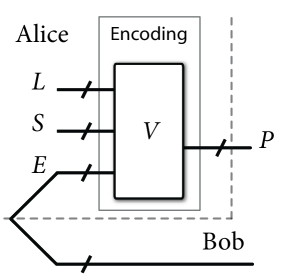
Figure 1: The encoder of an EAQ code. Alice acts on her logical qubits $L\,$, local ancillas $S$, and her halves of the ebits $E$ with an encoding unitary $V$. This encoding produces physical qubits $P$ that she then inputs to a noisy quantum channel. The entanglement-assisted paradigm assumes that noise does not occur on Bob’s half of the ebits, but we later study this setting in some simulations because it could occur in practice.

Suppose now that Alice transmits her $n$ qubits of the encoded state $\mathopen{}\mathclose{{}\left|\overline{\psi}}\right\rangle^{AB}$ over a noisy Pauli channel. Then the resulting state is $P^{A}\mathopen{}\mathclose{{}\left|\overline{\psi}}\right\rangle^{AB}$ where $P^{A}$ is some $n$-fold tensor product of Pauli operators (in what follows, we simply say an “$n$-qubit Pauli operator”). Suppose that Bob applies the inverse $\mathopen{}\mathclose{{}\left(V^{A}}\right)^{{\dagger}}$ of the encoding to the state $P^{A}\mathopen{}\mathclose{{}\left|\overline{\psi}}\right\rangle^{AB}$. The resulting state has the following form:

$$(V^{A})^{{\dagger}}P^{A}\mathopen{}\mathclose{{}\left|\overline{\psi}}\right\rangle^{AB} =(V^{A})^{{\dagger}}P^{A}V^{A}(\mathopen{}\mathclose{{}\left|\psi}\right\rangle^{A}\otimes\mathopen{}\mathclose{{}\left|0_{a}}\right\rangle^{A}\otimes\mathopen{}\mathclose{{}\left|\Phi_{c}^{+}}\right\rangle^{AB})$$

$$=L^{A}\mathopen{}\mathclose{{}\left|\psi}\right\rangle^{A}\otimes S^{A}\mathopen{}\mathclose{{}\left|0_{a}}\right\rangle^{A}\otimes E^{A}\mathopen{}\mathclose{{}\left|\Phi_{c}^{+}}\right\rangle^{AB}),$$ (1)

where $L^{A}$ is some $k$-qubit Pauli operator, $S^{A}=S_{1}^{A}\otimes\cdots\otimes S_{a}^{A}$ is an $a$-qubit Pauli operator, and $E^{A}=E_{1}^{A}\otimes\cdots\otimes E_{c}^{A}$ is some $c$-qubit Pauli operator. Observe that

$$S^{A}\mathopen{}\mathclose{{}\left|0_{a}}\right\rangle^{A}=\mathopen{}\mathclose{{}\left|s_{1}}\right\rangle^{A}\otimes\cdots\otimes\mathopen{}\mathclose{{}\left|s_{a}}\right\rangle^{A},$$

where $s_{i}=0$ if $S_{i}\in\mathopen{}\mathclose{{}\left\{I,Z}\right\}$ and $s_{i}=1$ otherwise. The fact that $s_{i}$ is invariant under the application of a Pauli $Z$ operator implies that a quantum code can be degenerate (where two different errors mapping to the same syndrome have the same effect on the encoded state). Also, observe that

$$E^{A}\mathopen{}\mathclose{{}\left|\Phi_{c}^{+}}\right\rangle^{AB}=\mathopen{}\mathclose{{}\left|\Phi\mathopen{}\mathclose{{}\left(e_{1,x},e_{1,z}}\right)}\right\rangle^{AB}\otimes\cdots\otimes\mathopen{}\mathclose{{}\left|\Phi\mathopen{}\mathclose{{}\left(e_{c,x},e_{c,z}}\right)}\right\rangle^{AB},$$

where $\mathopen{}\mathclose{{}\left|\Phi\mathopen{}\mathclose{{}\left(e_{i,x},e_{i,z}}\right)}\right\rangle^{AB}$ denotes the four distinguishable Bell states and

$$\mathopen{}\mathclose{{}\left(e_{i,x},e_{i,z}}\right) =\mathopen{}\mathclose{{}\left(0,0}\right)\text{ if }E_{i}^{A}=I,$$

$$\mathopen{}\mathclose{{}\left(e_{i,x},e_{i,z}}\right) =\mathopen{}\mathclose{{}\left(0,1}\right)\text{ if }E_{i}^{A}=Z,$$

$$\mathopen{}\mathclose{{}\left(e_{i,x},e_{i,z}}\right) =\mathopen{}\mathclose{{}\left(1,0}\right)\text{ if }E_{i}^{A}=X,$$

$$\mathopen{}\mathclose{{}\left(e_{i,x},e_{i,z}}\right) =\mathopen{}\mathclose{{}\left(1,1}\right)\text{ if }E_{i}^{A}=Y.$$

Thus all four Pauli operators are distinguishable in this case by performing a Bell measurement (similar to the super-dense coding effect [36]). Ebits do not contribute to the degeneracy of a quantum code because different errors $E^{A}$ lead to distinct measurement results.

Bob can perform $Z$ basis measurements on the ancillas and Bell measurements on the ebits to determine the syndrome $r\mathopen{}\mathclose{{}\left(P}\right)$ of the Pauli error $P$:

$$r\mathopen{}\mathclose{{}\left(P}\right)\equiv\mathopen{}\mathclose{{}\left(s_{1},\ldots,s_{a},e_{1,x},e_{1,z},\ldots,e_{c,x},e_{c,z}}\right).$$

Consider the following relation between the binary representations of $P$, $V$, $L$, $S$, and $E$ in (1):

$$PV^{-1}=\mathopen{}\mathclose{{}\left(L:S:E}\right).$$

The syndrome $r\mathopen{}\mathclose{{}\left(P}\right)$ only partially determines $S$, but it fully determines $E$. Let us decompose the binary representation of $S$ as $S=S^{z}+S^{x}$ and that of $E$ as $E=E^{z}+E^{x}$. When Bob performs his measurements, he determines $S^{x}$, $E^{z}$, and $E^{x}$. That is, he determines the following relations between the components $S_{i}^{x}$ of $S^{x}$ and the components $s_{i}$ of the syndrome $r\mathopen{}\mathclose{{}\left(P}\right)$:

$$S_{i}^{x}=X\text{ if }s_{i}=1,\ \ \ \ S_{i}^{x}=I\text{ otherwise.}$$

The syndrome also determines the $i^{\text{th}}$ components $E_{i}^{x}$ and $E_{i}^{z}$ of $E$:

$$E_{i}^{x} =X\text{ if }e_{i,x}=1,\ \ \ \ E_{i}^{x}=I\text{ otherwise,}$$

$$E_{i}^{z} =Z\text{ if }e_{i,z}=1,\ \ \ \ E_{i}^{z}=I\text{ otherwise.}$$

The phenomenon of degeneracy represents the most radical departure of quantum coding from classical coding [32, 33]. Consider two different physical errors $P$ and $P^{\prime}$ that differ only by $Z$ operators acting on the ancillas:

$$P =(L:S^{x}+S^{z}:E^{x}+E^{z})V$$

$$P^{\prime} =(L:S^{x}+S^{\prime z}:E^{x}+E^{z})V$$

$$=P+(I_{k}:S^{z}+S^{\prime z}:I_{c})V,$$

where $I_{k}$ is a length $2k$ zero vector (the binary representation of a $k$-fold tensor product of identity operators). These different errors lead to the same error syndrome. In the classical world, this would present a problem for error correction. But this situation does not cause a problem in the quantum world for the errors $P$ and $P^{\prime}$—the logical error affecting the encoded quantum information is the same for both $P$ and $P^{\prime}$, and Bob can correct either of these errors simply by applying $L^{-1}$ after decoding.

We now define several sets of operators that are important for determining the properties and performance of EAQ codes. The set $C\mathopen{}\mathclose{{}\left(I}\right)$ of harmless, undetected errors consists of all operators $P$ that have a zero syndrome, yet have no effect on the encoded state:

$$C\mathopen{}\mathclose{{}\left(I}\right)\equiv\mathopen{}\mathclose{{}\left\{P:P=(I_{k}:S^{z}:I_{c})V,\ \ S^{z}\in\mathopen{}\mathclose{{}\left\{I,Z}\right\}^{a}}\right\}.$$

This set of operators is equivalent to the isotropic subgroup, in the language of Refs. [19, 20]. It is also analogous to the all-zero codeword of a classical code. The set $C\mathopen{}\mathclose{{}\left(L}\right)$ of harmful, undetected errors consists of all operators $P$ that have a zero syndrome, yet change the quantum information in the encoded state:

$$C\mathopen{}\mathclose{{}\left(L}\right)\equiv\mathopen{}\mathclose{{}\left\{P:P=(L:S^{z}:I_{c})V,\ \ S^{z}\in\mathopen{}\mathclose{{}\left\{I,Z}\right\}^{a}}\right\},$$

where$\ L\neq I_{k}$. This set of operators corresponds to a single logical transformation on the encoded state, depending on the choice of $L$, and it is analogous to a single codeword of a classical code. The set $C\mathopen{}\mathclose{{}\left(L,S^{x},E^{x},E^{z}}\right)$ corresponds to a particular logical transformation and syndrome, and is thus a logical coset:

$$C\mathopen{}\mathclose{{}\left(L,S^{x},E^{x},E^{z}}\right)\\ \equiv\mathopen{}\mathclose{{}\left\{P:P=(L:S^{z}+S^{x}:E^{z}+E^{x})V,\ \ S^{z}\in\mathopen{}\mathclose{{}\left\{I,Z}\right\}^{a}}\right\}.$$

It is analogous to a single erred codeword of a classical code if $S^{x}$, $E^{x}$, or $E^{z}$ is non-zero. The operator codewords of an EAQ code belong to the following set $C$:

$$C\equiv\bigcup\limits_{L}C\mathopen{}\mathclose{{}\left(L}\right),$$ (2)

where $L$ is an arbitrary $k$-qubit Pauli operator. The set $C$ is equivalent to the full set of logical operators for the code, and it is analogous to the set of all codewords of a classical code. These definitions lead to the definition of the minimum distance of an EAQ code as the minimum weight of an operator $P$ in $C-C\mathopen{}\mathclose{{}\left(I}\right)$:

$$d\mathopen{}\mathclose{{}\left(C}\right)\equiv\min\mathopen{}\mathclose{{}\left\{w\mathopen{}\mathclose{{}\left(P}\right):P\in C-C\mathopen{}\mathclose{{}\left(I}\right)}\right\}.$$

This definition is similar to the definition of the distance of a classical code, but it incorporates the coset structure of a quantum code. Thus, we can determine the performance of the code in terms of distance by tracking its logical operators, and this intuition is important when we move on to EAQ convolutional codes. Also, the logical operators play an important role in decoding because a maximum likelihood decoding algorithm for a quantum code estimates the most likely logical error given the syndrome and a particular physical noise model.

We end this section with a final remark concerning EAQ codes and the musing of Hayden et al. in Ref. [26]. Suppose that an EAQ code does not exploit any ancilla qubits and uses only ebits. Then the features of the code become remarkably similar to that of a classical code. Degeneracy, a uniquely quantum feature of a code, does not occur in this case because the syndrome completely determines the error, in analogy with error correction in the classical world. Also, the code loses its coset structure, so that $C\mathopen{}\mathclose{{}\left(I}\right)$ is equal to the identity operator, $C\mathopen{}\mathclose{{}\left(L}\right)$ is equivalent to just one logical operator, and the definition of the code’s minimum distance is the same as the classical definition.

IV EAQ convolutional codes

An EAQ convolutional code is a particular type of EAQ code that has a convolutional structure. In past work on this topic [23, 24, 39], we adopted the “Grassl-Rötteler” approach to this theory [40], by beginning with a mathematical description of the code and determining a Grassl-Rötteler pearl-necklace encoder that can encode it. Here, we adopt the approach of Poulin et al. [6] which in turn heavily borrows from ideas in classical convolutional coding [13]. We begin with a seed transformation (a “convolutional encoder” or a “quantum shift-register circuit”) and determine its state diagram, which yields important properties of the encoder. We can always rearrange a Grassl-Rötteler pearl-necklace encoder as a convolutional encoder [41, 42, 43], but it is not clear that every convolutional encoder admits a form as a Grassl-Rötteler pearl necklace encoder. For this reason and others, we adopt the Poulin et al. approach in what follows.

An EAQ convolutional encoder is a “Clifford group” unitary $U$ that acts on $m$ memory qubits, $k$ information qubits, $a$ ancilla qubits, and $c$ halves of ebits to produce a set of $m$ memory qubits and$\ n$ physical or channel qubits, where $n=k+a+c$. The transformation that it induces on binary representations of Pauli operators acting on these registers is as follows:

$$\mathopen{}\mathclose{{}\left(M^{\prime}:P}\right)=(M:L:S:E)U,$$

where $M^{\prime}$ acts on the $m$ output memory qubits, $P$ acts on the $n$ output physical qubits, $M$ acts on the $m$ input memory qubits, $L$ acts on the $k$ information qubits, $S$ acts on the $a$ ancilla qubits, and $E$ acts on the $c$ halves of ebits. Although the quantum states in these registers can be continuous in nature, the act of syndrome measurement discretizes the errors acting on them, and the above classical representation is useful for analysis of the code’s properties and the flow of the logical operators through the encoding circuit (recall that the goal of a decoding algorithm is to produce good estimates of logical errors). This representation is similar to the shift-register representation of classical convolutional codes, with the difference that the representation there corresponds to the actual flow of bit information through a convolutional circuit, while here it is merely a useful tool for analyzing the properties of the encoder.

The overall encoding operation for the code is the transformation induced by repeated application of the above seed transformation to a quantum data stream broken up into periodic blocks of information qubits, ancilla qubits, and halves of ebits while feeding the output memory qubits of one transformation as the input memory qubits of the next (see Figure 6 of Ref. [6] for a visual aid). The advantage of a quantum convolutional encoder is that the complexity of the overall encoding scales only linearly with the length of the code for a fixed memory size, while the decoding complexity scales linearly with the length of the code by employing a local maximum likelihood decoder combined with a belief propagation algorithm [6]. The quantum communication rate of the code is essentially $k/n$ while the entanglement consumption rate is $c/n$, if the length of the code becomes large compared to $n$.

IV-A State Diagram

The state diagram of an EAQ convolutional encoder is the most important tool for analyzing its properties, and it is the formal quantization of a classical convolutional encoder’s state diagram [13, 14]. It examines the flow of the logical operators through the encoder with a finite-state machine approach, and this representation is important for analyzing both its distance and its performance under the iterative decoding algorithm of Ref. [6]. The state diagram is a directed multigraph with $4^{m}$ vertices that we think of as memory states. We label each memory state with an $m$-qubit Pauli operator $M$. We connect two vertices with a directed edge from $M\rightarrow M^{\prime}$, labeled as $\mathopen{}\mathclose{{}\left(L,P}\right)$, if there exists a $k$-qubit Pauli operator $L$, an $n$-qubit Pauli operator $P$, and an $a$-qubit Pauli operator $S^{z}\in\mathopen{}\mathclose{{}\left\{I,Z}\right\}^{a}$ such that

$$\mathopen{}\mathclose{{}\left(M^{\prime}:P}\right)=(M:L:S^{z}:I_{c})U.$$ (3)

We refer to the labels $L$ and $P$ of an edge as the respective logical and physical label.

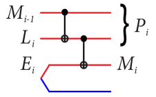
Figure 2: (Color online) Seed transformation for an $n=2$, $k=1$, $c=1$, $m=1$ EAQ convolutional code.

As an example, consider the transformation depicted in Figure 2. It acts on one memory qubit, one information qubit, and one half of an ebit to produce two channel qubits and one memory qubit. Figure 3 illustrates the state diagram corresponding to this transformation. There are four memory states because there is only one memory qubit, and there are 16 edges because there are four memory states and four logical operators for one information qubit and one ebit.

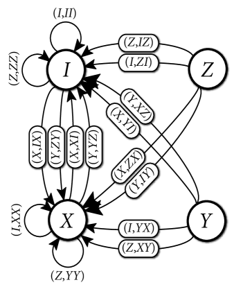
Figure 3: The state diagram corresponding to the seed transformation in Figure 2. The state diagram allows us to check that the encoder is non-catastrophic and non-recursive.

IV-B Non-catastrophicity

We now recall the definition of non-catastrophicity in Ref. [6], which is the formal quantization of the definition in Section IX of Ref. [13]. The definition from Ref. [6] is the same for an EAQ convolutional encoder because it depends on the iterative decoding algorithm used to decode the code, and we can exploit a slight variation of the iterative decoding algorithm in Ref. [6] to decode EAQ convolutional codes. A path through the state diagram is a sequence $M_{1}$, …, $M_{t}$ of vertices such that $M_{i}\rightarrow M_{i+1}$ is an edge belonging to it. Each logical operator of $C$ in (2) corresponds to a path in the state diagram, with the sequence of vertices in the path being the states of memory traversed while encoding the logical operator. The physical and logical weights of a logical operator are equal to the sums of the corresponding weights of the edges traversed in a path that encodes the logical operator. A zero physical-weight cycle is a cycle in the state diagram such that all edges in the cycle have zero physical weight. Finally, an EAQ encoder acting on $m$ memory qubits, $k$ information qubits, $a$ ancilla qubits, and $c$ ebits is non-catastrophic if every zero physical-weight cycle in its state diagram has zero logical weight.

Why is this definition an appropriate definition of non-catastrophicity? First, suppose that we modify the circuit in Figure 2 so that the ebit is replaced by an ancilla qubit (it thus becomes the same as Figure 8 of Ref. [6]). Such a replacement leads to a doubling of the number of edges in the state diagram in our Figure 3 because the state diagram should include all of the transitions where a $Z$ operator acts on the ancilla qubits (these all lead to other logical operators in their case). The new state diagram (see Figure 9 of Ref. [6]) then includes a self-loop at memory state $Z$ with zero physical weight and non-zero logical weight, and it is thus catastrophic according to the definition. The problem with such a loop is that it can “throw off” the iterative decoding algorithm. If a $Y$ error were to act on the second physical qubit in one frame of the code (while the identity acts on the rest), then “pushing” this error through the inverse of the encoder applies an $X$ operator to the ancilla qubit and produces one syndrome bit for that frame of the code, but it propagates $Z$ errors onto every logical qubit in the stream while applying $Z$ errors to every memory qubit. All of these other errors go undetected by an iterative decoder because the error propagation does not trigger any additional syndrome bits besides the initial one that the $Y$ error triggered.

Observe that the state diagram in Figure 3 for the EAQ convolutional encoder does not feature a zero physical-weight cycle with non-zero logical weight. Thus, the encoder is non-catastrophic, illustrating another departure from the classical theory of turbo codes. Non-catastrophicity in the quantum world is not only a property of the encoder, but it also depends on the resources available for encoding. If we analyze the above scenario that leads to catastrophic error propagation in the unassisted encoder, we see that it does not lead to such propagation for the entanglement-assisted encoder in Figure 2. Indeed, suppose again that a $Y$ error acts on the second physical qubit in a particular frame of the code (with the identity acting on all other qubits). Pushing this $Y$ error through the inverse of the encoder leads to an $X$ operator acting on the ebit and a $Z$ operator acting on the memory. The $X$ operator is detectable by a Bell measurement, and the $Z$ operator acting on the memory propagates to a $Z$ operator acting on an ebit in the next frame and then to all ebits and information qubits in successive frames. These $Z$ operators acting on the ebits are all detectable by a Bell measurement (whereas they are not detecable when acting on an ancilla), so that the iterative decoding algorithm can still correct for errors in the propagation because all these errors trigger syndromes.

IV-C Recursiveness

Recursiveness is another desirable property for an EAQ convolutional encoder when it is employed as the inner encoder of a quantum serial turbo code. This property ensures that a quantum serial turbo code on average has a distance growing near-linearly with the length of the code, and a proof of this statement given in Ref. [16] is essentially a direct translation of the classical proof [5]. In short, an EAQ convolutional encoder is quasi-recursive if it transforms every weight-one Pauli operator $X_{i}$, $Y_{i}$, or $Z_{i}$ to an infinite-weight Pauli operator [6]. It is recursive if, in addition to being quasi-recursive, every element in the logical cosets $C\mathopen{}\mathclose{{}\left(X_{i}}\right)$, $C\mathopen{}\mathclose{{}\left(Y_{i}}\right)$, and $C\mathopen{}\mathclose{{}\left(Z_{i}}\right)$ has infinite weight. This stringent requirement is necessary due to the coset structure of EAQ codes. One might think that quasi-recursiveness is a sufficient requirement for good performance, but our simulation results in Section VIII indicate that recursiveness is indeed necessary because a turbo code has a significant increase in performance if its inner encoder is recursive.

It seems like it would be demanding to determine if this condition holds for every possible input, but we can exploit the state diagram to check it. The algorithm for checking recursiveness is as follows. First, we define an admissable path to be a path in which its first edge is not part of a zero physical-weight cycle [6]. Now, consider any vertex belonging to a zero-physical weight loop and any admissable path beginning at this vertex with logical weight one. The encoder is recursive if all such paths do not contain a zero physical-weight loop [6]. The idea is that a weight-one logical operator is not sufficient to drive a recursive encoder to a memory state that is part of a zero-physical weight loop—the minimum weight of a logical operator that does so is two.

The example encoder in Figure 2 is not recursive. The only vertex in the state diagram in Figure 3 belonging to a zero physical-weight cycle is the vertex labeled $I$. If the logical input to the encoder is a $Z$ operator followed by an infinite sequence of identity operators, the circuit outputs $ZZ$ as the physical output, returns to the memory state $I$, and then outputs the identity for the rest of time. Thus, the response to this weight-one input is finite, and the circuit is non-recursive. Although this example is non-recursive, Section V details many examples of EAQ convolutional encoders that are both recursive and non-catastrophic.

IV-D Distance Spectrum

We end this section by reviewing the performance measures from Ref. [6], which are also quantizations of the classical measures [13]. The distance spectrum $F\mathopen{}\mathclose{{}\left(w}\right)$ of an EAQ convolutional encoder is the number of admissable paths beginning and ending in memory states that are part of a zero physical-weight cycle, where the physical weight of each admissable path is $w$ and the logical weight is greater than zero. This performance measure is most similar to the weight enumerator polynomial of a quantum block code [44], which helps give an upper bound on the error probability of a non-degenerate quantum code on a depolarizing channel under maximum likelihood decoding [45]. The distance spectrum incorporates the translational invariance of a quantum convolutional code and gives an indication of its performance on a memoryless depolarizing channel. Appendix A details a simple method to compute the distance spectrum by using the state diagram and ideas rooted in Refs. [13, 46, 47, 48]. The free distance of an EAQ convolutional encoder is the smallest weight $w$ for which $F\mathopen{}\mathclose{{}\left(w}\right)>0$, and this parameter is one indicator of the performance of a quantum serial turbo code employing constituent convolutional encoders. Although one of the applications of our EAQ convolutional encoders are as the inner encoders in a quantum serial turbo coding scheme, we can also have them as outer encoders in a quantum serial turbo code and use the free distance to show that its minimum distance grows near-linearly when combined with a non-catastrophic, recursive inner encoder.

V Example Encoders

Our first example of an EAQ convolutional encoder is the simplest example that is both recursive and non-catastrophic. It exploits one memory qubit and one ebit to encode one information qubit per frame. We discuss this first example in detail, verifying its non-catastrophicity and recursiveness, and we give a method to compute its distance spectrum. Appendix B then gives tables that detail our other examples. We found all of these examples by picking encoders uniformly at random from the Clifford group, according to the algorithm in Section VI-A.2 of Ref. [49].

The seed transformation for our first example is as follows:

$$\begin{array}[c]{ccc}Z&I&I\\ I&Z&I\\ I&I&Z\\ X&I&I\\ I&X&I\\ I&I&X\end{array}\rightarrow\begin{array}[c]{ccc}Z&I&X\\ X&Z&Y\\ X&Y&Z\\ X&X&X\\ Y&I&Y\\ Y&X&Y\end{array},$$ (4)

where the first input qubit is the memory qubit, the second input qubit is the information qubit, the third is Alice’s half of the ebit, the first output qubit is the memory qubit, and the last two outputs are the physical qubits. We can abbreviate the above encoding by taking the binary representation of each row at the output and encoding it as a decimal number. For example, the first row $ZIX$ has the binary representation $\mathopen{}\mathclose{{}\left[\mathopen{}\mathclose{{}\left.\begin{array}[c]{ccc}1&0&0\end{array}}\right|\begin{array}[c]{ccc}0&0&1\end{array}}\right]$ which is the decimal number 33. Thus, we can specify this encoder as $\mathopen{}\mathclose{{}\left\{33,29,30,7,45,47}\right\}$.

The seed transformation in (4) leads to the state diagram of Figure 4, by exploiting (3). We can readily check that the encoder is non-catastrophic and recursive by inspecting Figure 4. The only cycle with zero physical weight is the self-loop at the identity memory state with zero logical weight. The encoder is thus non-catastrophic. To verify recursiveness, note again that the only vertex belonging to a zero physical-weight cycle is the self-loop at the identity memory state. We now consider all weight-one admissable paths that begin in this state. If we input a logical $X$, we follow the edge $\mathopen{}\mathclose{{}\left(X,IY}\right)$ to the $Y$ memory state. Inputting the identity operator for the rest of time keeps us in the self-loop at memory state $Y$ while still outputting non-zero physical weight operators. We can then check that inputting a $Z$ logical operator followed by identities keeps us in the self-loop at the $X$ memory state while still outputting non-zero physical weight operators, and inputting a $Y$ logical operator followed by identities keeps us in the self-loop at the $Z$ memory state. The encoder is thus recursive. Appendix B lists many more examples of entanglement-assisted quantum convolutional encoders that are both recursive and non-catastrophic.

Figure 4: The state diagram corresponding to the seed transformation in (4), acting on one memory qubit, one information qubit, one ebit, and producing two physical qubits. The above state diagram allows us to check that the encoder is both recursive and non-catastrophic.

VI EAQ Turbo Codes

We comment briefly on the construction and minimum distance of a quantum serial turbo code that employs our example encoders as a constituent encoder (the next section details our simulation results with different encoders). The construction of an EAQ serial turbo code is the same as that in Ref. [6] (see Figure 10 there), with the exception that we assume that Alice and Bob share entanglement in the form of ebits before encoding begins. Alice first encodes her stream of information qubits with the outer encoder, performs a quantum interleaver on all of the qubits, and then encodes the resulting stream with the inner encoder. The quantum communication rate of the resulting EAQ turbo code is $k^{\text{Out}}/n^{\text{In}}=(k^{\text{Out}}/n^{\text{Out}})(k^{\text{In}}/n^{\text{In}})$ where $k^{\text{Out}}$ is the number of information qubits encoded by the outer encoder, $n^{\text{Out}}$ is the number of physical qubits output from the outer encoder, and a similar convention holds for $k^{\text{In}}$, $n^{\text{In}}$, and the inner encoder. In order for the qubits to match up properly, $n^{\text{Out}}$ must be equal to $k^{\text{In}}$. The entanglement consumption rate of the code is $(c^{\text{Out}}+c^{\text{In}})/n^{\text{In}}$ where $c^{\text{Out}}$ and $c^{\text{In}}$ are the total number of ebits consumed by the outer and inner encoder, respectively.

Perhaps the best combination for an EAQ serial turbo code is to choose the inner quantum convolutional encoder to be a recursive, non-catastrophic EAQ convolutional encoder and the outer quantum convolutional encoder to be a non-recursive, non-catastrophic standard quantum convolutional encoder. This combination reduces entanglement consumption, ensures good iterative decoding performance, and ensures that the minimum distance of the quantum serial turbo code grows as $N^{\mathopen{}\mathclose{{}\left(d^{\ast}-2}\right)/d^{\ast}}$ where $N$ is the length of the code and $d^{\ast}$ is the free distance of the outer quantum convolutional encoder. A proof of this last statement given in Ref. [16] is essentially identical to the classical proof [5]. Section VIII-A shows that this combination also performs well in practice if noise occurs on the ebits. Additionally, choosing the outer quantum convolutional encoder to encode a highly degenerate code may increase the number of errors that the quantum turbo code can correct, in a vein similar to the results in Ref. [33] (though we have not yet fully investigated this possibility). Appendix B lists many examples of entanglement-assisted quantum turbo codes and discusses their average minimum distance scaling.

VII Incorporating Extrinsic Information into the Quantum Turbo Decoding Algorithm

Poulin et al. proposed an iterative decoding algorithm for quantum turbo codes in Ref. [6]. Their algorithm is based on the exchange of a posteriori information between the constituent quantum convolutional decoders of a quantum turbo code. Since the decoders pass along a posteriori information, successive iterations of the constituent decoders are dependent on one another, and this gives rise to a detrimental positive feedback effect, which prevents the decoding algorithm there from achieving the desired gains usually observed in iterative decoding.

To avoid the aforementioned situation, it is necessary to ensure that the a priori information directly related to a given information qubit is not reused in the other constituent decoder [1, 50]. Similar to the approach employed in classical turbo decoding [1, 51], this can be achieved by having one decoder remove a priori information from the a posteriori information before feeding it to the other decoder. More explicitly, the iterative decoding procedure should exchange only “extrinsic” information which is unknown and new to the other decoder.

To see how this works, let us consider a four-port Soft-Input Soft-Output (SISO) decoder [51, 52] that generates soft output information pertaining to a logical error $L$ and physical error $P$. As shown in Figure 5, a SISO decoder exploits an A Posteriori Probability (APP) module that accepts the a priori information $\mathbf{P}^{a}(L)$ and $\mathbf{P}^{a}(P)$ as input and outputs the a posteriori information $\mathbf{P}^{o}(L)$ and $\mathbf{P}^{o}(P)$. The corresponding extrinsic probabilities $\mathbf{P}^{e}(L^{j}_{i})$ and $\mathbf{P}^{e}(P^{j}_{i})$ for the $j^{\text{th}}$ qubit at time instant $i$ are then obtained by discarding the a priori information from the a posteriori information as follows [51, 52]:

$$\mathbf{P}^{e}(L^{j}_{i})=N_{L^{j}}\frac{\mathbf{P}^{o}(L^{j}_{i})}{\mathbf{P}^{a}(L^{j}_{i})},$$

$$\mathbf{P}^{e}(P^{j}_{i})=N_{P^{j}}\frac{\mathbf{P}^{o}(P^{j}_{i})}{\mathbf{P}^{a}(P^{j}_{i})},$$ (5)

where $N_{L^{j}}$ and $N_{P^{j}}$ are normalization factors, which ensure that $\sum_{L^{j}}\mathbf{P}^{e}(L^{j}_{i})=1$ and $\sum_{P^{j}}\mathbf{P}^{e}(P^{j}_{i})=1$, respectively. Furthermore, to avoid any numerical instabilities and to reduce the computational complexity, log-domain arithmetics are conventionally employed, which convert the multiplicative operations of (5) to addition, as given below [52]:

$$\ln[\mathbf{P}^{e}(L^{j}_{i})] =\ln[\mathbf{P}^{o}(L^{j}_{i})]-\ln[\mathbf{P}^{a}(L^{j}_{i})],$$

$$\ln[\mathbf{P}^{e}(P^{j}_{i})] =\ln[\mathbf{P}^{o}(P^{j}_{i})]-\ln[\mathbf{P}^{a}(P^{j}_{i})].$$ (6)

Therefore, the inputs and outputs of a SISO decoder are the logarithmic a priori and extrinsic probabilities, respectively.

Figure 5: A SISO decoder processes soft a piori information to yield soft extrinsic information which is useful for iterative decoding. The quantities $\mathbf{P}^{a}(\cdot)$, $\mathbf{P}^{e}(\cdot)$ and $\mathbf{P}^{o}(\cdot)$ denote the a priori, extrinsic and a posteriori probabilities, while $L$ and $P$ denote the logical and physical errors.

Based on the above discussion, we have modified the turbo decoding algorithm of Ref. [6] so that the constituent decoders pass along only extrinsic information to each other. See Figure 6 for a depiction of the modified quantum turbo decoding algorithm [53]. In this figure, $A(y)$ and $E(y)$ denote the logarithmic a priori and extrinsic probabilities of $y$, where $y\in\{L_{1},L_{2},P_{1},P_{2}\}$. Analogous to Ref. [6], the inner SISO decoder of Figure 6 exploits the physical noise model $A(P_{1})$, syndrome $S^{x}_{1}$ and a priori information $A(L_{1})$, the last of which is initialized to be equiprobable. However, it outputs the extrinsic information $E(L_{1})$, rather than the a posteriori information as in Ref. [6]. The extrinsic information $E(L_{1})$ is then interleaved to serve as the a priori information $A(P_{2})$ for the outer SISO decoder. The two decoders thereby engage in iterative decodings, which continue until either the a posteriori probability $E(L_{2})$ converges to a definite solution, or a prespecified maximum number of iterations is reached.

Figure 6: Schematic of the quantum turbo decoder algorithm that exploits extrinsic information rather than a posteriori information as in Ref. [6]. In the above, $A(\cdot)$ and $E(\cdot)$ denote the logarithmic a priori and extrinsic probabilities, $L_{i}$ and $P_{i}$ are the logical and physical errors, while $S^{x}_{i}$ represents the $X$-syndrome for the $i^{\text{th}}$ decoder. The generalization of this algorithm to the entanglement-assisted case is straightforward.

VIII Simulation Results

We performed several simulations of EAQ turbo codes and detail the results in this section. This section begins with a description of the parameters of the constituent quantum convolutional encoders. We then describe how the simulation was run, and we finally discuss and interpret the simulation results.

Our simulation results presented here are certainly not intended to be an exhaustive comparison of codes, but they rather serve to illustrate the enhancement in performance from the modified algorithm described in Section VII and they constitute an exploration of the effect of adding entanglement assistance to the encoders of Poulin et al. [6]—our original intent was to exploit their encoders, but the lack of a clear exposition of their decimal representation convention has excluded us from doing so. So we instead randomly generated and filtered encoders that have comparable attributes to their encoders. The first encoder, dubbed “PTO1R,” acts on three input memory qubits, one information qubit, and two ancillas to produce three output memory qubits and three physical qubits. Its decimal representation is

$$\begin{array}[c]{c}\{1355,2847,558,2107,3330,739,\\ \ \ \ 2009,286,473,1669,1979,189\}\end{array},$$

and a truncated distance spectrum polynomial (see Appendix A) for it is

$$11x^{5}+47x^{6}+253x^{7}+1187x^{8}+\\ 6024x^{9}+30529x^{10}+153051x^{11}+771650x^{12}.$$

This encoder is non-catastrophic and quasi-recursive, and its parameters and distance spectrum are comparable to those of Poulin et al.’s first encoder (though they did not comment on whether theirs is quasi-recursive) [6]. Replacing the two ancilla qubits in the encoder with two ebits gives an improvement in its truncated distance spectrum polynomial:

$$2x^{9}+x^{10}+5x^{11}+8x^{12}+11x^{13}+25x^{14}+\\ 56x^{15}+102x^{16}+217x^{17}+387x^{18}+787x^{19}.$$

The encoder also becomes recursive after this replacement. Let “PTO1REA” denote the EA version of this encoder.

Our second encoder, dubbed “PTO3R,” acts on four input memory qubits, one information qubit, and one ancilla qubit to produce four output memory qubits and two physical qubits. Its decimal representation is

$$\begin{array}[c]{c}\{3683,3556,2872,2211,3561,3534,\\ \ \ \ 729,3136,743,2643,1330,1656\}\end{array},$$

and a truncated distance spectrum polynomial for it is

$$12x^{5}+93x^{6}+600x^{7}+4320x^{8}+31098x^{9}+\\ 224014x^{10}+1604435x^{11}+11469935x^{12}.$$

The encoder is non-catastrophic and quasi-recursive with its parameters and distance spectrum comparable to those of Poulin et al.’s third encoder. Replacing the ancilla with an ebit gives an improvement to the truncated distance spectrum polynomial:

$$x^{6}+3x^{7}+7x^{8}+29x^{9}+88x^{10}+237x^{11}+\\ 716x^{12}+2166x^{13}+6245x^{14}+18696x^{15}+\\ 55889x^{16}+165971x^{17}+492805x^{18}+1465529x^{19},$$

and the encoder becomes recursive after this replacement. Let “PTO3REA” denote the EA version of the “PTO3” encoder.

Our turbo codes consist of interleaved serial concatenation of the above encoders with themselves, and we varied the auxiliary resources of the encoders to be ebits, ancillas, or both. Concatenating PTO1R with itself leads to a rate 1/9 quantum turbo code, and concatenating PTO3R with itself leads to a rate 1/4 turbo code.

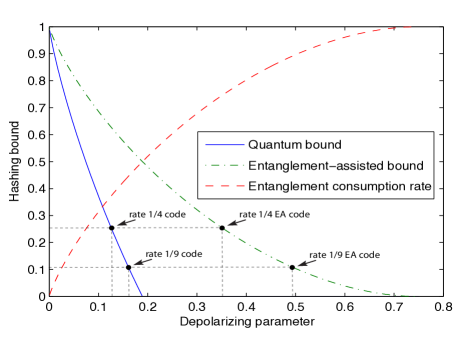
Figure 7: The figure plots the hashing bound for quantum codes (solid blue curve), the entanglement-assisted hashing bound for EAQ codes (the dash-dotted green curve), and the entanglement consumption rate of the father protocol that meets the entanglement-assisted hashing bound (dashed red curve). The figure plots these different bounds as a function of the depolarizing parameter $p$. Observe that the noise limit for a rate 1/4 quantum code is $\approx 0.12689$, the noise limit for a rate 1/9 quantum code is $\approx 0.16028$, the noise limit for a rate 1/4 EAQ code is $\approx 0.35454$, and the noise limit for a rate 1/9 EAQ code is $\approx 0.49088$. We should compare our simulation results with these noise limits to observe how close our code constructions come to achieving the quantum capacity (though note that the unassisted hashing bound is only a lower bound on the unassisted quantum capacity [32, 33]).

We simulated the performance of these EAQ turbo codes on a memoryless depolarizing channel with parameter $p$. The action of the channel on a single qubit density operator $\rho$ is as follows:

$$\rho\rightarrow\mathopen{}\mathclose{{}\left(1-p}\right)\rho+\frac{p}{3}\mathopen{}\mathclose{{}\left(X\rho X+Y\rho Y+Z\rho Z}\right).$$

The benchmarks for the performance of any standard or entanglement-assisted quantum code on a depolarizing channel are the hashing bounds [54, 21]. The quantum hashing bound determines the rate at which a random quantum code can operate reliably for a particular depolarizing parameter $p$, but note that it does not give the ultimate capacity limit because degeneracy can improve performance [33, 55, 56, 57]. On the other hand, the entanglement-assisted hashing bound does give the ultimate capacity at which an EAQ code can operate reliably for a particular depolarizing parameter $p$, whenever an unbounded amount of entanglement is available [21, 38]. The hashing bound for quantum communication is

$$1-\mathopen{}\mathclose{{}\left[H_{2}\mathopen{}\mathclose{{}\left(p}\right)+p\log_{2}\mathopen{}\mathclose{{}\left(3}\right)}\right],$$

and the hashing bound for an entanglement-assisted quantum code is

$$1-\frac{1}{2}\mathopen{}\mathclose{{}\left[H_{2}\mathopen{}\mathclose{{}\left(p}\right)+p\log_{2}\mathopen{}\mathclose{{}\left(3}\right)}\right].$$ (7)

The father protocol is a quantum communication protocol that achieves the entanglement-assisted quantum capacity [58, 59, 60], while attempting to minimize its entanglement consumption rate. Its entanglement consumption rate is provably optimal for certain channels such as the dephasing channel [61, 62, 63], but it is not necessarily optimal for the depolarizing channel. The entanglement consumption rate of the father protocol on a depolarizing channel is

$$\frac{1}{2}\mathopen{}\mathclose{{}\left[H_{2}\mathopen{}\mathclose{{}\left(p}\right)+p\log_{2}\mathopen{}\mathclose{{}\left(3}\right)}\right].$$

This entanglement consumption rate implies that the only resources involved in an encoded transmission of the father protocol are information qubits and ebits because the sum of its quantum communication rate and its entanglement consumption rate is equal to one. Figure 7 plots these different hashing bounds and depicts the location of these bounds for our different quantum turbo codes.

One can also consider a “hashing region” of rates that are achievable for entanglement-assisted quantum communication [59, 58, 64]—this region is the more relevant benchmark for an entanglement-assisted code that does not consume the maximal amount of entanglement. For the case of a depolarizing channel, this region consists of all $Q$ and $E$ that satisfy the following bounds:

$$Q \leq 1-\mathopen{}\mathclose{{}\left[H_{2}\mathopen{}\mathclose{{}\left(p}\right)+p\log_{2}\mathopen{}\mathclose{{}\left(3}\right)}\right]+E$$ (8)

$$Q \leq 1-\frac{1}{2}\mathopen{}\mathclose{{}\left[H_{2}\mathopen{}\mathclose{{}\left(p}\right)+p\log_{2}\mathopen{}\mathclose{{}\left(3}\right)}\right],$$ (9)

where $Q$ is the quantum communication rate and $E$ is the entanglement consumption rate. The intersection of these two boundary lines occurs when $E=\frac{1}{2}\mathopen{}\mathclose{{}\left[H_{2}\mathopen{}\mathclose{{}\left(p}\right)+p\log_{2}\mathopen{}\mathclose{{}\left(3}\right)}\right]$, the entanglement consumption rate of the father protocol. When an entanglement-assisted quantum code does not consume the maximal amount of entanglement possible (but rather at some rate $E\leq\frac{1}{2}\mathopen{}\mathclose{{}\left[H_{2}\mathopen{}\mathclose{{}\left(p}\right)+p\log_{2}\mathopen{}\mathclose{{}\left(3}\right)}\right]$), we should compare its performance with the boundary in (8).

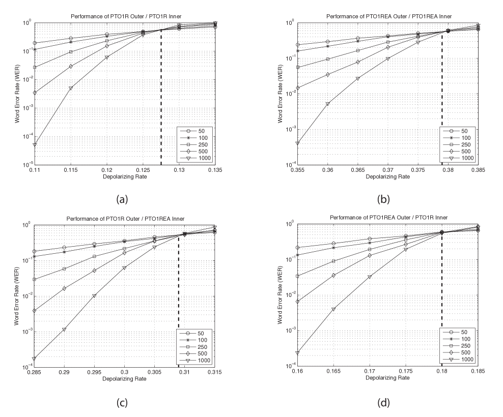
Figure 8: The figure plots the results of four different simulations that exploit the PTO1R and PTO1REA encoders. The resulting EAQ turbo codes have rate 1/9 and varying entanglement consumption rates. Each plot demonstrates the existence of a threshold, where the code performance increases whenever the channel noise rate is below the threshold. The vertical dotted line in each plot indicates the approximate location of the threshold.

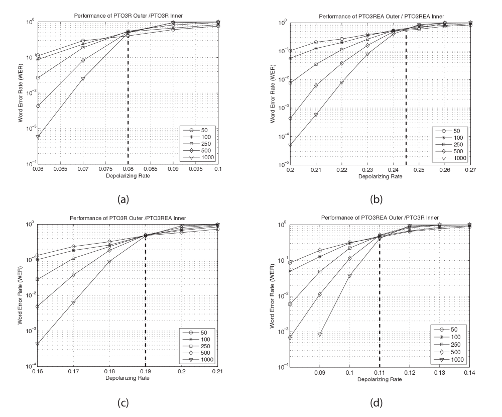
Figure 9: The figure plots the results of four different simulations that exploit the PTO3R and PTO3REA encoders. The resulting EAQ turbo codes have rate 1/4 and varying entanglement consumption rates. Each plot demonstrates the existence of a threshold, where the code performance increases whenever the channel noise rate is below the threshold. The vertical dotted line in each plot indicates the approximate location of the threshold.

We performed Monte Carlo simulations to determine the performance of our example EAQ turbo codes when decoded with an iterative decoding algorithm (the iterative decoding algorithm is as described in Section VII, with the exception that it decodes EAQ turbo codes). We developed a Matlab computer program for these simulations [65].

A single run of a simulation selects a quantum turbo code with a particular number of logical qubits and a random choice of interleaver, and it then generates a Pauli error randomly according to a depolarizing channel with parameter $p$. This Pauli error leads to an error syndrome, and the syndrome and channel model act as inputs to the iterative decoding algorithm. The iterative decoding algorithm terminates if the hard decision on a recovery operation is the same decision from the previous iteration, or it terminates after a maximum number of iterations (though we never observed the number of iterations until convergence exceeding eight). One run of the simulation declares a failure if the estimated recovery operation is different from the correct recovery operation. The ratio of simulation failures to the total number of simulation runs is the word error rate (WER). In the cases in which errors occur more rarely, we ran every configuration (choice of code, depolarizing parameter, and number of logical qubits) until we observed at least 100 failures—this number gaurantees a reasonable statistical confidence in the results of the simulations. Of course, in the cases where errors occur more frequently, we observed thousands of errors.

Our first simulation involved the serial concatenation of the unassisted PTO1R encoder with itself, and Figure 8(a) displays the results. The performance significantly exceeds that of the first encoder of Poulin et al. (see Figure 12 of Ref. [6]) and there is an improved separation between the curves for increasing blocklength, when comparing Figure 8(a) to Figure 12 of Ref. [6]. A noticeable feature of Figure 8(a) is the existence of a pseudothreshold, such that increasing the number of encoded qubits of the turbo code decreases the WER for all depolarizing noise rates below the pseudothreshold. The pseudothreshold is not a true threshold because this particular turbo code has a bounded minimum distance, and at some point, the WER should begin increasing if we continue to increase the number of encoded qubits [6]. The pseudothreshold occurs at a depolarizing noise rate $\approx 0.1275$, and this pseudothreshold is within $0.994$ dB of the $0.16028$ noise limit for a rate $1/9$ code.

Our second simulation tested the serial concatenation of the PTO1REA encoder with itself, and Figure 8(b) displays the results. This turbo code uses the maximal amount of entanglement at a rate of $8/9$ and thus is an instance of the so-called “father” protocol. Entanglement assistance gives the turbo code a dramatic increase in performance, in the sense that it can withstand far higher depolarizing noise rates than the unassisted turbo code. The threshold occurs at $\approx 0.379$—we call this a threshold rather than a pseudothreshold because we expect that the WER should continue to decrease as we increase the number of encoded qubits, but we should clarify that we have not proven that this should hold. However, the EXIT chart analysis of Ref. [53] suggests that this is a true threshold. This threshold is $4.73$ dB beyond the pseudothreshold of the unassisted turbo code, and it is within $1.12$ dB of the $0.49088$ noise limit given by the EA hashing bound in (7) for a qubit rate $1/9$ and ebit rate $8/9$ code. This code construction is operating in a noise regime in which standard quantum codes are simply not able to operate (compare with the results in Refs. [66, 67, 68, 6, 69, 70, 71, 72]).

Our third simulation tested the serial concatenation of the PTO1REA inner encoder with the PTO1R outer encoder, and this EAQ turbo code has an entanglement consumption rate of $6/9$. The benchmark for comparison is given by (8), so that for a code with qubit rate $1/9$ and ebit rate $6/9$, its noise limit is found by solving for the $p$ for which

$$1/9-6/9=-5/9=1-\mathopen{}\mathclose{{}\left[H_{2}\mathopen{}\mathclose{{}\left(p}\right)+p\log_{2}\mathopen{}\mathclose{{}\left(3}\right)}\right],$$

which in this case is $p\approx 0.3779$. The inner encoder is recursive, but the outer encoder’s free distance is not as high as that in the previous simulation. Figure 8(c) displays the results. The threshold occurs approximately at a depolarizing noise rate of $0.309$, which is within $0.887$ dB of the previous threshold and within $0.87$ dB of the $0.3779$ noise limit given above.

Our final simulation tested the serial concatenation of the PTO1R inner encoder with the PTO1REA outer encoder, and this EAQ turbo code has an entanglement consumption rate of $2/9$. Again, the benchmark for comparison is given by (8), so that for a code with qubit rate $1/9$ and ebit rate $2/9$, its noise limit is found by solving for the $p$ for which

$$1/9-2/9=-1/9=1-\mathopen{}\mathclose{{}\left[H_{2}\mathopen{}\mathclose{{}\left(p}\right)+p\log_{2}\mathopen{}\mathclose{{}\left(3}\right)}\right],$$

which in this case is $p\approx 0.2209$. The inner encoder is quasi-recursive, and the outer encoder has a significantly higher free distance than in the previous simulation because it has entanglement assistance. Though, one can place a constant upper bound on the minimum distance of these turbo codes because the inner encoder is not recursive. This simulation provides a good test to determine the effectiveness of an inner encoder that is quasi-recursive. That is, one might think that quasi-recursiveness of the inner encoder combined with an outer encoder with high free distance would be sufficient to produce a turbo code with good performance (the thought is that this would explain the good performance in the first simulation), but Figure 8(d) suggests that this intuition does not hold. The pseudothreshold occurs at approximately $0.18$. This pseudothreshold is only $1.50$ dB higher than the threshold for the unassisted code, and it is $0.889$ dB away from the noise limit of $0.2209$ given above.

We conducted similar simulations with the PTO3R and PTO3REA encoders, and Figures 9(a-d) display the results. The entanglement consumption rates in Figures 9(a-d) are $0$, $3/4$, $2/4$, and $1/4$, respectively. The results are somewhat similar to the previous simulations with the difference that the noise limits and thresholds are lower because these codes have higher quantum data transmission rates. The thresholds occur at approximately $0.08$, $0.245$, $0.19$, and $0.11$ in Figures 9(a-d), respectively, and the hashing limits for these codes are approximately $0.1268$, $0.3545$, $0.2636$, and $0.1893$, respectively. Thus, these codes are within 2 dB, 1.6 dB, 1.4 dB, and 2.35 dB of their hashing limits, respectively. Since the threshold of the code in Figure 9(c) occurs at $0.19$, so that it is performing closest to its hashing limit (1.4 dB away), it appears that this EAQ turbo code is making judicious use of the available entanglement by placing the two ebits in the inner encoder. We would have to conduct further simulations to determine if placing one ebit in the outer encoder and one in the inner encoder would do better, but our suspicion is that the aforementioned use of entanglement is better because the inner encoder is recursive under this choice.

VIII-A Noise on Ebits

We conducted another set of simulations to determine how noise on Bob’s half of the ebits affects the performance of a code. This possibility has long been one of the important practical questions concerning the entanglement-assisted paradigm, and some researchers have provided partial answers [73, 74, 75, 76, 78]. We briefly review some of these contributions. Shaw et al. first observed that the $\mathopen{}\mathclose{{}\left[\mathopen{}\mathclose{{}\left[7,1,3}\right]}\right]$ Steane code is equivalent to a $\mathopen{}\mathclose{{}\left[\mathopen{}\mathclose{{}\left[6,1,3;1}\right]}\right]$ entanglement-assisted code that can also correct a single error on Bob’s half of the ebit. This observation goes further: any standard, non-degenerate $\mathopen{}\mathclose{{}\left[\mathopen{}\mathclose{{}\left[n,k,d}\right]}\right]$ quantum code is equivalent to an $\mathopen{}\mathclose{{}\left[\mathopen{}\mathclose{{}\left[n-d+1,k,d;d-1}\right]}\right]$ entanglement-assisted code that can correct any $\mathopen{}\mathclose{{}\left\lfloor\mathopen{}\mathclose{{}\left(d-1}\right)/2}\right\rfloor$ errors on Alice and Bob’s qubits. This result holds because tracing over any $n-d+1$ qubits in the original standard code gives a maximally mixed state on $d-1$ qubits, and the purification of these qubits are $n-d+1$ encoded halves of ebits that Alice possesses [77]. Lai and Brun have studied this observation in more detail, by conducting simulations of such entanglement-assisted codes, and they have also studied the case in which a standard stabilizer code is used to protect the ebits [78]. Wilde and Fattal observed that entanglement-assisted codes correcting for errors on Bob’s side slightly improve the threshold for quantum computation if ebit errors occur less frequently than gate errors [74]. Hsieh and Wilde studied this question in the Shannon-theoretic context and determined an expression for capacity when channel errors and entanglement errors occur [75]. As a side note, Lai and Brun have also looked for codes attempting to achieve the opposite goal [37]—their codes try to maximize the number of channel errors that can be corrected while minimizing the correction on Bob’s half of the ebits.

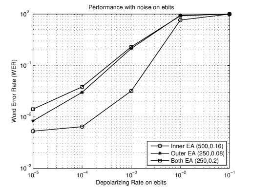
Figure 10: The figure plots the performance of different inner and outer encoder combinations as a function of noise rate on Bob’s half of the ebits. The number of logical qubits and channel noise for each combination is indicated in the figure legend. It is surprising that the combination PTO3REA inner / PTO3R outer can withstand more ebit noise than the combination PTO3R inner / PTO3REA outer even though it uses more ebits than this latter combination.

Figure 10 plots the results of our simulations that allow for noise on Bob’s half of the ebits. We performed three different types of simulations: the first was with the PTO3REA inner / PTO3R outer combination, the second with the PTO3R inner / PTO3REA outer combination, and the third with the PTO3REA inner / PTO3REA outer combination. For each simulation, we kept the channel noise rates fixed at $0.16$, $0.08$, and $0.2$, respectively, because the codes already performed reasonably well at these noise rates, and our goal was to understand the effect of ebit noise on code performance. The codes all performed about the same as they did without ebit noise if we set the ebit noise rate at $10^{-5}$. Increasing the ebit noise rate an order of magnitude to $10^{-4}$ has the least effect on the PTO3REA inner / PTO3R outer combination. Increasing it further to $10^{-3}$ deteriorates the performance of the other combinations while still having the least effect on the PTO3REA inner / PTO3R outer combination. This result is surprising, considering that this combination has an entanglement consumption rate of $2/4$ while the entanglement consumption rate of the PTO3R inner / PTO3REA outer combination is smaller at $1/4$. The result suggests that it would be wiser to place ebits in the inner encoder rather than in the outer encoder when these codes operate in practice.

Figure 11 seems to confirm this suggestion. Increasing the number of logical qubits to 1000 for each combination shows an increased performance for the combination PTO3REA inner / PTO3R outer if the ebit noise level is not too high, while the other two combinations perform worse. It is surprising that the combination PTO3REA inner / PTO3R outer performs better—increasing the number of logical qubits in turn increases the number of ebits, having more ebits should translate into more noise on the syndromes, and this then should affect performance. However, this particular combination seems to exhibit some amount of robustness against ebit noise if it is not too high.

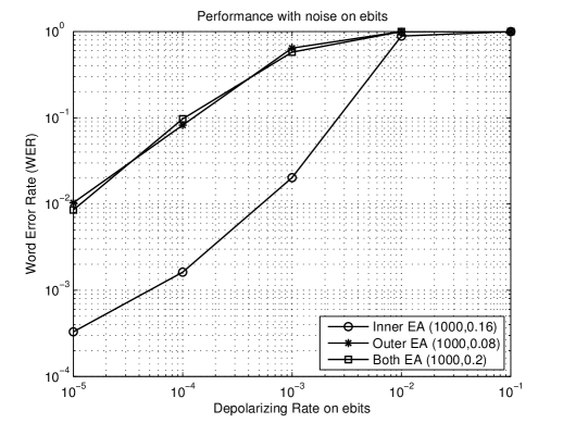
Figure 11: The figure again plots the performance of different inner and outer encoder combinations as a function of noise rate on Bob’s half of the ebits, though we increased the number of logical qubits in each combination to be 1000. Interestingly, the combination PTO3REA inner / PTO3R outer shows an increased performance after increasing the number of logical qubits to 1000, at least for ebit noise levels at $10^{-3}$ or below. The other combinations perform worse after increasing the number of logical qubits to 1000.

IX Recursive, Classically-Enhanced Subsystem Encoders are Catastrophic

We can construct other variations of quantum convolutonal encoders and study their state diagrams to determine their properties. One example of a variation mentioned at the end of Ref. [6] is a subsystem convolutional code (based on the idea of a subsystem quantum code [79, 80, 81] that is useful in fault-tolerant quantum computation [82]). Poulin et al. suggest that subsystem convolutional codes might be “a concrete avenue” for circumventing the inability of a quantum convolutional encoder to be simultaneously recursive and non-catastrophic. Such codes exploit a resource known as a “gauge” qubit that can add extra degeneracy beyond that available in a standard stabilizer code. Another variation is an encoder that encodes both classical bits and qubits, and we might wonder if these could be simultaneously recursive and non-catastrophic (such codes are known as “classically-enhanced” codes [83] and are based on trade-off coding ideas from quantum Shannon theory [84]).

Unfortunately, encoders that act on logical qubits, classical bits, ancilla qubits, and gauge qubits cannot possess both properties simultaneously, and we state this result below as a corollary of Theorem 1 in Ref. [6]. This result implies that entanglement is the resource enabling a convolutional encoder to be both recursive and non-catastrophic (there are no other known local resources for quantum codes besides ancilla qubits, classical bits, and gauge qubits).

Corollary 1

Suppose that a classically-enhanced subsystem convolutional encoder is recursive. Then it is catastrophic.

Proof:

First, consider that the state diagram for a classically-enhanced subsystem quantum convolutional encoder includes an edge from $M$ to $M^{\prime}$ if there exists a $k_{q}$-qubit Pauli operator $L_{q}\in\mathopen{}\mathclose{{}\left\{I,X,Y,Z}\right\}^{k_{q}}$, an $a$-qubit Pauli operator $S^{z}\in\mathopen{}\mathclose{{}\left\{I,Z}\right\}^{a}$, a $k_{c}$-qubit Pauli operator $L_{c}^{x}+C^{z}\in\mathopen{}\mathclose{{}\left\{I,X,Y,Z}\right\}^{k_{c}}$, and a $g$-qubit Pauli operator $G^{x}+G^{z}\in\mathopen{}\mathclose{{}\left\{I,X,Y,Z}\right\}^{g}$ such that

$$\mathopen{}\mathclose{{}\left(M^{\prime}:P}\right)=(M:L_{q}:S^{z}:L_{c}^{x}+C^{z}:G^{x}+G^{z})U,$$ (10)

where the binary representations of Pauli operators are the same as in (3). We break the operator acting on the $k_{c}$ classical bits into two parts because $L_{c}^{x}$ represents the $X$ component of the operator that can flip a classical bit from $\mathopen{}\mathclose{{}\left|0}\right\rangle$ to $\mathopen{}\mathclose{{}\left|1}\right\rangle$ and back, while $C^{z}$ represents the $Z$ component of the operator that has no effect on a classical bit in state $\mathopen{}\mathclose{{}\left|0}\right\rangle$ or $\mathopen{}\mathclose{{}\left|1}\right\rangle$ (it merely adds an irrelevant global phase in the case that the bit is equal to $\mathopen{}\mathclose{{}\left|1}\right\rangle$). The entries $G^{x}$ and $G^{z}$ are for the “gauge qubits” in a subsystem code [81] (qubits in a maximally mixed state that are invariant under the random application of an arbitrary Pauli operator). We include these transitions in the state diagram because a particular logical operator $L\equiv\mathopen{}\mathclose{{}\left(L_{q}:L_{c}^{x}}\right)$ in a classically-enhanced subsystem code is equivalent up to $Z$ operators acting on the ancilla qubits, $Z$ operators acting on the classical bits, and $X$ and $Z$ operators acting on gauge qubits. The set $C\mathopen{}\mathclose{{}\left(L}\right)$ corresponding to a particular logical input $L\equiv\mathopen{}\mathclose{{}\left(L_{q}:L_{c}^{x}}\right)$ consists of all operators $P$ of the following form:

$$C\mathopen{}\mathclose{{}\left(L}\right)\equiv\mathopen{}\mathclose{{}\left\{\begin{array}[c]{c}P:P=(L_{q}:S^{z}:L_{c}^{x}+C^{z}:G^{x}+G^{z})V,\\ S^{z}\in\mathopen{}\mathclose{{}\left\{I,Z}\right\}^{a},\ \ C^{z}\in\mathopen{}\mathclose{{}\left\{I,Z}\right\}^{k_{c}},\\ G^{x}+G^{z}\in\mathopen{}\mathclose{{}\left\{I,X,Y,Z}\right\}^{g}\end{array}}\right\},$$

where $V$ in this case consists of the infinite, repeated, overlapping application of the convolutional encoder $U$.

Suppose that the encoder is recursive. By definition, it follows that every weight-one logical input $L$ and its coset $C\mathopen{}\mathclose{{}\left(L}\right)$ has an infinite response. Suppose now that we change the resources in the encoder so that all of the classical bits and gauge qubits become ancilla qubits. The resulting code is now a standard stabilizer code. Additionally, we can remove the $X$ operators $L_{c}^{x}$ from the definition of $C\mathopen{}\mathclose{{}\left(L}\right)$ because they no longer play a role as a logical operator, and we can remove the $X$ operators $G^{x}$ from the definition of $C\mathopen{}\mathclose{{}\left(L}\right)$ because they are acting on ancilla qubits. Let $C^{\prime}\mathopen{}\mathclose{{}\left(L^{\prime}}\right)$ denote the new set corresponding to a particular logical operator $L^{\prime}\equiv\mathopen{}\mathclose{{}\left(L_{q}:I_{k_{c}}}\right)$:

$$C^{\prime}\mathopen{}\mathclose{{}\left(L^{\prime}}\right)\equiv\mathopen{}\mathclose{{}\left\{\begin{array}[c]{c}P:P=(L_{q}:S^{z}:C^{z}:G^{z})V,\\ S^{z}\in\mathopen{}\mathclose{{}\left\{I,Z}\right\}^{a},\ \ C^{z}\in\mathopen{}\mathclose{{}\left\{I,Z}\right\}^{k_{c}},\\ G^{z}\in\mathopen{}\mathclose{{}\left\{I,Z}\right\}^{g}\end{array}}\right\}.$$

The encoder is still recursive because $C^{\prime}\mathopen{}\mathclose{{}\left(L^{\prime}}\right)\subset C\mathopen{}\mathclose{{}\left(L^{\prime}}\right)$ and because the original encoder is recursive (recursiveness is a property invariant under the replacement of cbits and gauge qubits with ancilla qubits). Then Theorem 1 of Ref. [6] implies that the encoder for the stabilizer code is catastrophic, i.e., it features a zero physical-weight cycle with non-zero logical weight. It immediately follows that the original encoder for the classically-enhanced subsystem code is catastrophic because its state diagram contains all of the edges of the stabilizer encoder, plus additional edges that correspond to the logical transitions for the classical bits and the $X$ operators acting on the gauge qubits. ∎

We should note that the above argument only holds if the original classically-enhanced subsystem convolutional encoder acts on a non-zero number of logical qubits (this of course is the case in which we are really interested in order to have a non-zero quantum communication rate). For example, the encoder in Figure 2 becomes recursive and non-catastrophic when replacing the logical qubit with a classical bit and the ebit with an ancilla. One can construct the state diagram from the specification in (10) and discover that these two properties hold for the encoder acting on the cbit and ancilla.

The above argument also does not apply if an ebit is available as an auxiliary resource for an encoder. We have found an example of a non-catastrophic, recursive encoder that acts on six memory qubits, one logical qubit, one ancilla qubit, one ebit, one cbit, and one gauge qubit. The seed transformation for this example is as follows:

$$\begin{array}[c]{c}\{2934387,3034525,2323986,3804870,964819,2111270,\\ \ \ \ 3722470,1017852,2678995,912985,1575948,3138834,\\ \ \ \ 142503,317898,3473283,1492935,2701400,2492844,\\ \ \ \ 2078030,1894781,915544,75029\}.\end{array}$$

A non-catastrophic, non-recursive subsystem convolutional encoder with a high free distance could potentially serve well as an outer encoder of a quantum turbo code, but this might not necessarily be beneficial if our aim is to achieve the capacity of a quantum channel. The encoder for a subsystem code is effectively a noisy encoding map because it is a unitary acting on information qubits in a pure state, ancilla qubits in a pure state, and gauge qubits in the maximally mixed state. Ref. [61] proves that an isometric encoder is sufficient to attain capacity, and we can thus restrict our attention to subspace codes rather than subsystem codes. Though, this line of reasoning does not rule out the possibility that iterative decoding could somehow benefit from the extra degeneracy available in a subsystem code, but this extra degeneracy would increase the decoding time.

X Classically-Enhanced EAQ Encoders

We might also wish to construct classically-enhanced EAQ turbo codes that transmit classical information in addition to quantum information, in an effort to reach the optimal trade-off rates from quantum Shannon theory [61, 62]. These codes are then based on the structure of the codes in Refs. [83, 85]. The state diagram for the encoder includes an edge from $M$ to $M^{\prime}$ if there exists a $k_{q}$-qubit Pauli operator $L_{q}\in\mathopen{}\mathclose{{}\left\{I,X,Y,Z}\right\}^{k_{q}}$, a $k_{c}$-qubit Pauli operator $L_{c}^{x}\in\mathopen{}\mathclose{{}\left\{I,X}\right\}^{k_{q}}$, a $k_{c}$-qubit Pauli operator $L_{c}^{z}\in\mathopen{}\mathclose{{}\left\{I,Z}\right\}^{k_{q}}$, and an $a$-qubit Pauli operator $S^{z}\in\mathopen{}\mathclose{{}\left\{I,Z}\right\}^{a}$ such that

$$\mathopen{}\mathclose{{}\left(M^{\prime}:P}\right)=(M:L_{q}:S^{z}:L_{c}^{x}+L_{c}^{z}:I_{c})U.$$

The logical operator $L_{q}$ acts on $k_{q}$ qubits while the operator $L_{c}^{x}+L_{c}^{z}$ acts on $k_{c}$ classical bits. We break this latter operator into two parts for the same reason discussed in the previous section. The state diagram for an encoder of this form is similar to that for an EAQ convolutional encoder because it includes all transitions for the classical bits. The difference is in the interpretation of the logical weight of edge transitions and in the logical label of an edge. If an edge features a $Z$ operator acting on a classical bit, then this operator does not contribute to the logical weight of the transition and does not appear on the logical labels—an $I$ appears on the logical label if $I$ or $Z$ acts on the classical bit and an $X$ appears on the logical label if an $X$ or $Y$ acts on it.

We have found several examples of recursive, non-catastrophic encoders acting on these resources. One of our examples acts on five memory qubits, one logical qubit, one ancilla qubit, one ebit, and one classical bit. Its seed transformation is as follows:

$$\begin{array}[c]{c}\{162568,174333,260907,261622,168521,3644,\\ 101236,204504,227699,260074,138781,9252,\\ 257257,179548,78687,6352,230925,180362\}.\end{array}$$

XI The Preservation of Recursiveness and Non-Catastrophicity under Resource Substitution

The technique used to prove Corollary 1 motivates us to consider which resource substitutions preserve the properties of recursiveness and non-catastrophicity. We have two different cases:

1. A resource substitution that removes edges from the state diagram preserves non-catastrophicity and recursiveness.

2. A resource substitution that adds edges to the state diagram preserves catastrophicity and non-recursiveness.

To see the first case for recursiveness preservation, consider a general encoder acting on logical qubits, ancilla qubits, ebits, cbits, and gauge qubits. Each logical input $L\equiv\mathopen{}\mathclose{{}\left(L_{q}:L_{c}^{x}}\right)$ to the encoder has the following form:

$$C\mathopen{}\mathclose{{}\left(L}\right)\equiv\mathopen{}\mathclose{{}\left\{\begin{array}[c]{l}P:\\ P=(L_{q}:S^{z}:I_{c}:L_{c}^{x}+C^{z}:G^{x}+G^{z})V,\\ S^{z}\in\mathopen{}\mathclose{{}\left\{I,Z}\right\}^{a},\ \ C^{z}\in\mathopen{}\mathclose{{}\left\{I,Z}\right\}^{k_{c}},\\ G^{x}+G^{z}\in\mathopen{}\mathclose{{}\left\{I,X,Y,Z}\right\}^{g}\end{array}}\right\},$$

where the conventions are similar to what we had before. Suppose the encoder is recursive so that $C\mathopen{}\mathclose{{}\left(X_{i}:I}\right)$, $C\mathopen{}\mathclose{{}\left(Y_{i}:I}\right)$, $C\mathopen{}\mathclose{{}\left(Z_{i}:I}\right)$, and $C\mathopen{}\mathclose{{}\left(I:X_{j}}\right)$ all have an infinite response. Then the encoder is still recursive if we replace an ancilla with an ebit because the original encoder is recursive and we no longer have to consider the $Z$ operator acting on the replaced ancilla. The encoder is still recursive if we replace a cbit with an ancilla qubit because we no longer have to consider the coset $C\mathopen{}\mathclose{{}\left(I:X_{j}}\right)$. Finally, it is still recursive if we replace a gauge qubit with an ancilla qubit because we no longer have to consider the $X$ operator acting on the replaced gauge qubit.

To see the first case for non-catastrophicity preservation, suppose that an encoder is already non-catastrophic. Then a resource substitution that removes edges from the state diagram preserves non-catastrophicity because this removal cannot create a zero physical-weight cycle with non-zero logical weight.

To see the second case for non-recursiveness preservation, suppose that an encoder acting on logical qubits and ebits is non-recursive, meaning that at least one of the weight-one logical inputs $X_{i}$, $Y_{i}$, or $Z_{i}$ has a finite response. Then replacing an ebit with an ancilla certainly cannot make the resulting encoder recursive because we have to consider the response to the operators $X_{i}$, $Y_{i}$, or $Z_{i}$ and one of these is already finite from the assumption of non-recursiveness of the original encoder. Furthermore, consider a non-recursive encoder acting on logical qubits, ebits, and ancilla qubits. Replacing some of the ancilla qubits with cbits or gauge qubits cannot make the encoder become recursive for the same reasons.

To see the second for catastrophicity preservation, suppose that an encoder is catastrophic. Then a resource substitution that adds edges to the state diagram preserves catastrophicity because any zero physical-weight cycles with non-zero logical weight are still part of the state diagram for the new encoder.

The following diagram summarizes all of the above observations. The resources are $L$ for logical qubits, $S$ for ancilla qubits, $E$ for ebits, $C$ for cbits, and $G$ for gauge qubits. Recursiveness and non-catastrophicity preservation flow downwards under the displayed resource substitutions, while non-recursiveness and catastrophicity preservation flow upwards (substitutions at the same level can go in any order).

$($	$L$	$:$	$S$	$:$	$E$	$:$	$C$	$:$	$G$	$)$
			$\downarrow\uparrow$				$\downarrow\uparrow$		$\downarrow\uparrow$
$($	$L$	$:$	$E$	$:$	$E$	$:$	$S$	$:$	$S$	$)$
							$\downarrow\uparrow$		$\downarrow\uparrow$
$($	$L$	$:$	$E$	$:$	$E$	$:$	$E$	$:$	$E$	$)$

We can then understand the proof of Corollary 1 in the context of the above diagram. The original encoder acts on $\mathopen{}\mathclose{{}\left(L:S:C:G}\right)$ and is assumed to be recursive. Resource substitution of $C$ and $G$ preserves recursiveness, while making the encoder act on only ancilla qubits (the auxiliary resource for a standard quantum code). Using the fact that standard recursive quantum encoders are catastrophic [6], we then back substitute the resources, which is a catastrophicity preserving substitution.

XII Conclusion and Current Work

We have constructed a theory of EAQ serial turbo coding as an extension of Poulin et al.’s theory in Ref. [6]. The introduction of shared entanglement simplifies the theory because an EAQ convolutional encoder can be both recursive and non-catastrophic. These two properties are essential for quantum serial turbo code families to have minimum distance that grows near-linearly with the length of the code, while still performing well under iterative decoding. We provided many examples of EAQ convolutional encoders that satisfy both properties, and we detailed their parameters. We then showed how the concatenation of these encoders with some of Poulin et al.’s and some of our own lead to EAQ serial turbo codes with near-linear minimum distance scaling. We modified the quantum turbo decoding algorithm from Ref. [6] such that it follows the turbo decoding principle in which the constituent decoders pass along extrinsic information, and this modification lead to a significant performance improvement over the algorithm outlined in Ref. [6]. We conducted several simulations of EAQ turbo codes—several of our quantum turbo codes were within 1 dB of their hashing limits and two notable surprises were that placing ebits in the inner encoder can achieve a better performance than expected in both scenarios with and without ebit noise. Our simulations are generally consistent with the findings in Ref. [39, 37] and other results from quantum Shannon theory [21, 59], namely, that entanglement assistance can significantly enhance error correction ability. Finally, we considered how to construct the state diagram for encoders that derive from other existing extensions to the theory of quantum error correction, and we showed that classically-enhanced subsystem convolutional encoders cannot simultaneously be recursive and non-catastrophic.

There are many questions to ask going forward from here. One could certainly seek out other entanglement-assisted quantum turbo codes and conduct numerical simulations of their performance. One purpose of our numerical simulations was to illustrate the effect of adding entanglement assistance to the encoders of Poulin et al. [6], and it was not our intent for them to constitute an exhaustive code comparison. It is ongoing work to search for and test many other code combinations, including cases where the inner and outer encoder are either recursive, non-recursive, have high / medium / low minimum distance, and have varying numbers of memory qubits $\leq 4$. Also, if one wished to compare directly the performance of entanglement-assisted turbo codes against the codes in Ref. [6], one way to do so might be to look for higher-rate codes operating near the entanglement-assisted hashing bound that tolerate the same noise level as the codes from Ref. [6]. One could also vary the number of ebits and ancilla qubits present in the various code combinations discussed here.

It would be interesting to explore the performance of the other suggested code structures in Section X to determine if they could come close to achieving the optimal rates from quantum Shannon theory [61, 62]. For example, what is the best arrangement for a classically-enhanced EAQ code? Should we place the classical bits in the inner or outer encoder? Are there more clever ways to use entanglement so that we increase error-correcting ability while reducing entanglement consumption? Consider that Hsieh et al. recently constructed a class of entanglement-assisted codes that exploit one ebit and still have good performance [86].

We should stress that the behavior of the entanglement-assisted codes using maximal entanglement is exactly like that of a classical turbo code. There is no degeneracy, and the iterative decoding algorithm is exactly the same as the classical one. Furthermore, analyses of classical turbo codes should apply directly in these cases [4, 87], and it would be good to determine the exact correspondence. These analyses studied the bit error rate rather than the word error rate, so any study of EAQ turbo codes would have to factor into account this difference.

Much of the classical literature has focused on the choice of a practical interleaver rather than a random one [88, 89, 90, 91], and it might be interesting to import the knowledge discovered here to the quantum case.

Finally, it would be great to find examples of EAQ turbo codes with a positive catalytic rate that outperform the turbo codes in Ref. [6], in the sense that they either have a higher catalytic rate while tolerating the same noise levels or they have the same catalytic rate while tolerating higher noise levels. This is ongoing work.

We acknowledge David Poulin for providing us with a copy of Ref. [16] and for many useful discussions, e-mail interactions, and feedback on the manuscript. We acknowledge Jean-Pierre Tillich for originally suggesting that shared entanglement might help in quantum serial turbo codes. We acknowledge Todd Brun, Hilary Carteret, and Jan Florjanczyk for useful discussions, and Patrick Hayden for the observation that non-degenerate quantum codes lead to entanglement-assisted codes with particular error correction power on Bob’s half of the ebits. Zunaira Babar is grateful to Prof. Lajos Hanzo and Dr. Soon Xin Ng (Michael) for their continuous guidance and support. We acknowledge the computer administrators in the McGill School of Computer Science for making their computational resources available for this scientific research. MMW acknowledges the warm hospitality of the ERATO-SORST project, the support of the MDEIE (Québec) PSR-SIIRI international collaboration grant, and the support of the Centre de Recherches Mathématiques in Montreal.

Appendix A Computing the Distance Spectrum

There is a straightforward way to compute the distance spectrum of a quantum convolutional encoder. This technique borrows from similar ideas in the classical theory of convolutional coding [13, 46, 47, 48]. We would like to know the number of admissible paths with a particular weight beginning and ending in memory states that are part of a zero physical-weight cycle. For our example in Section V, the identity memory state is the only memory state part of a zero physical-weight cycle. We create a weight adjacency matrix whose entries correspond to edges in the state diagram. This matrix has $x^{w}$ in entry $\mathopen{}\mathclose{{}\left(i,j}\right)$ if there is a physical-weight-$w$ edge from vertex $i$ to vertex $j$ (with the exception of the self-loop at the identity memory state). The weight adjacency matrix $A$ for our example is

$$A\equiv\begin{bmatrix}0&x^{2}&x&x\\ x^{2}&x^{2}&x^{2}&x^{2}\\ x^{2}&x&x&x^{2}\\ x^{2}&x&x^{2}&x\end{bmatrix},$$

where the ordering of vertices is $I$, $X$, $Y$, and $Z$. Note that we place a zero in the $\mathopen{}\mathclose{{}\left(1,1}\right)$ entry because we do not want to overcount the number of admissable paths starting and ending in memory states that are part of a zero physical-weight cycle. If we would like the number of admissable paths up to an arbitrary weight that start and end in the identity memory state, then we compute the $\mathopen{}\mathclose{{}\left(1,1}\right)$ entry of the following matrix:

$$\mathopen{}\mathclose{{}\left(I-A}\right)^{-1}=I+A+A^{2}+A^{3}+\cdots.$$

The coefficient of $x^{w}$ in the polynomial entry $\mathopen{}\mathclose{{}\left(I-A}\right)^{-1}\mathopen{}\mathclose{{}\left(1,1}\right)$ is the number of admissable paths with weight $w$ starting and ending in the identity memory state. One can compute this in some cases using Cramer’s rule, for example. We can also approximate the distance spectrum, e.g., by computing the matrix $B$ where

$$B=\sum_{i=1}^{T}A^{i},$$

and $T$ is some finite positive integer, so that this approximation gives a truncated distance spectrum. Computing the above matrix can be computationally expensive for large $T$, but we can dramatically reduce the number of computations by truncating the polynomial entries of $A$ above degree $T$ before performing each multiplication. For our example in Section V, the first ten entries of the distance spectrum polynomial are

$$2x^{3}+5x^{4}+6x^{5}+23x^{6}+54x^{7}+122x^{8}+298x^{9}+737x^{10},$$

so that this gives a fairly reasonable approximation to the true distance spectrum. These coefficients appear in the second column of Table II as the first ten values of the distance spectrum for this first example encoder. Note that there are faster ways of computing the distance spectrum for classical convolutional codes [92], and it remains open to determine how to exploit these techniques for quantum convolutional encoders.

Appendix B Example Encoders

Encoder	M	L	A	E	Seed Transformation	Free Dist.
1	1	1	0	1	$\{33,29,30,7,45,47\}$	3
2	3	2	0	1	$\mathopen{}\mathclose{{}\left\{2188,246,115,2053,1847,833,1658,2571,1566,2783,2990,3229}\right\}$	4
3	3	3	0	1	$\{12515,8790,10280,11314,6500,14691,1430,7105,8817,1420,10014,7061,10739,8972\}$	4
4	3	4	0	1	$\begin{array}[c]{c}\{23233,28350,13963,43904,58908,19553,6318,63573,\\ 12838,7558,22611,27045,48320,9596,48500,54018\}\end{array}$	3
5	2	1	1	1	$\{159,1006,727,641,925,522,726,314,793,648,119,210\}$	4
6	2	1	1	2	$\{1116,1363,1495,1326,241,2411,2268,1480,2032,1589,810,3351\}$	5
7	2	2	1	1	$\{141,509,3495,2470,2702,3576,1522,905,2622,1598,642,773\}$	3
8	2	6	0	1	$\begin{array}[c]{c}\{113633,199924,181760,243189,25748,110950,158559,282,205474,\\ 193680,199692,252779,245067,64266,147306,152171,230343,75396\}\end{array}$	2
9	2	8	0	1	$\begin{array}[c]{c}\{2432999,1503627,1816960,1050871,1297694,3894582,410463,2344289,1908709,\\ 3176421,3668357,1860207,1511167,3829280,3008050,2896381,999389,374648,\\ 4000734,885953,2452389,3608225\}\end{array}$	2
10	2	9	0	1	$\begin{array}[c]{c}\{4943947,12156608,10237254,2501342,2665695,7306816,8727132,80870,13726997,\\ 16078090,11897398,9857749,16524053,972786,5098459,8962232,10325041,\\ 12705543,8324846,13241728,11521711,7907747,16588769,5842661\}\end{array}$	N/A

TABLE I: Specification of our example EAQ convolutional encoders that are recursive and non-catastrophic. The first column indexes the different encoders, and all of the other columns correspond to a particular encoder. Column “M” gives the number of memory qubits, column “L” gives the number of information qubits, column “A” gives the number of ancilla qubits, and column “E” gives the number of ebits. The column labeled “Seed Transformation” specifies the seed transformation for each encoder, using a decimal representation. The convention for qubit ordering is that an encoder acts on memory qubits, information qubits, ancilla qubits, and ebits to produce output memory qubits and physical or channel qubits. The convention for the bit representation of a tensor product of Pauli operators is $ZXYZ$ maps to $[1011|0110]$, and the decimal representation of this bit vector is 182 (see the discussion around (4) in the text). The last column gives the free distance of the encoder.

Table I lists the specifications of many other examples of EAQ encoders that are both recursive and non-catastrophic—a computer program helped check that these properties hold for each of the examples [65]. Included in the list of example encoders are some which act on ancilla qubits in addition to ebits. These examples demonstrate that we do not necessarily require the auxiliary resource of an EAQ convolutional encoder to be ebits alone in order for the encoder to possess both properties. Table II gives a truncated distance spectrum for each of these encoders.

$w$	1	2	3	4	5	6	7
0	0	0	0	0	0	0	0
1	0	0	0	0	0	0	0
2	0	0	0	0	0	0	0
3	2	0	0	3	0	0	3
4	5	1	8	32	3	0	22
5	6	6	69	292	3	1	73
6	23	49	463	2,622	23	1	286
7	54	218	3,478	24,848	41	1	1,309
8	122	1,077	25,057	227,262	127	3	5,696
9	298	5,477	181,959	2.1$\cdot 10^{6}$	325	11	23,975
10	737	27,428	1,326,070	1.9$\cdot 10^{7}$	1,061	17	102,132

TABLE II: A truncated distance spectrum for the first seven of our example EAQ convolutional encoders. The first column on the left gives the first 11 values of the weight $w$, and the other columns give the first 11 values of the truncated distance spectrum $F(w)$ of the first seven of our EAQ convolutional encoders from Table I.

We can construct EAQ serial turbo codes, by serially concatenating some of our example “WH encoders” in Table I with the “PTO encoders” in Table 1 of Ref. [6] (ordered from left to right). Table III details these different combinations, giving their rates and average minimum distance scaling.

Outer	Inner	Q	E	Min. Dist.
PTO1	WH3	1/4	1/4	$N^{2/3}$
PTO2	WH3	1/4	1/4	$N^{5/7}$
PTO3	WH2	1/3	1/3	$N^{3/4}$
PTO3	WH7	1/4	1/4	$N^{3/4}$
PTO3	WH4	2/5	1/5	$N^{3/4}$
PTO2	WH8	2/7	1/7	$N^{5/7}$
PTO3	WH8	3/7	1/7	$N^{3/4}$
PTO3	WH9	4/9	1/9	$N^{3/4}$
PTO2	WH10	3/10	1/10	$N^{5/7}$
WH11	WH3	1/2	1/4	$N^{1/3}$

TABLE III: Various combinations of encoders for quantum turbo codes and their minimum distance scaling.

The columns of Table III give the outer encoder, the inner encoder, the quantum communication rate, the entanglement consumption rate, and the average minimum distance growth of a particular EAQ turbo code. The first four combinations all have a good average minimum distance scaling, but the catalytic rate for each of them is zero. The last six combinations both have a good average minimum distance scaling and a positive catalytic rate.

References

- [1] C. Berrou, A. Glavieux, and P. Thitimajshima, “Near Shannon limit error-correcting coding and decoding: Turbo-codes,” in Technical Program of the IEEE International Conference on Communications, vol. 2, Geneva, Switzerland, May 1993, pp. 1064–1070.
- [2] S. Benedetto and G. Montorsi, “Unveiling turbo codes: Some results on parallel concatenated coding schemes,” IEEE Transactions on Information Theory, vol. 42, no. 2, pp. 409–428, March 1996.
- [3] C. Berrou and A. Glavieux, “Near optimum error correcting coding and decoding: Turbo-codes,” IEEE Transactions on Communications, vol. 44, no. 10, pp. 1261–1271, October 1996.
- [4] S. Benedetto, D. Divsalar, G. Montorsi, and F. Pollara, “Serial concatenation of interleaved codes: performance analysis, design, and iterative decoding,” IEEE Transactions on Information Theory, vol. 44, no. 3, pp. 909–926, May 1998.
- [5] N. Kahale and R. Urbanke, “On the minimum distance of parallel and serially concatenated codes,” in Proceedings of the International Symposium on Information Theory, Cambridge, Massachussetts, USA, August 1998, p. 31. [Online]. Available: http://lthcwww.epfl.ch/{~}ruediger/papers/weight.ps
- [6] D. Poulin, J.-P. Tillich, and H. Ollivier, “Quantum serial turbo-codes,” IEEE Transactions on Information Theory, vol. 55, no. 6, pp. 2776–2798, June 2009.
- [7] S. Lloyd, “Capacity of the noisy quantum channel,” Physical Review A, vol. 55, no. 3, pp. 1613–1622, March 1997.
- [8] P. W. Shor, “The quantum channel capacity and coherent information,” in Lecture Notes, MSRI Workshop on Quantum Computation, 2002.
- [9] I. Devetak, “The private classical capacity and quantum capacity of a quantum channel,” IEEE Transactions on Information Theory, vol. 51, pp. 44–55, January 2005.
- [10] P. Hayden, M. Horodecki, A. Winter, and J. Yard, “A decoupling approach to the quantum capacity,” Open Systems & Information Dynamics, vol. 15, pp. 7–19, March 2008.
- [11] H. Ollivier and J.-P. Tillich, “Description of a quantum convolutional code,” Physical Review Letters, vol. 91, no. 17, p. 177902, October 2003.
- [12] G. D. Forney, M. Grassl, and S. Guha, “Convolutional and tail-biting quantum error-correcting codes,” IEEE Transactions on Information Theory, vol. 53, pp. 865–880, 2007.
- [13] A. J. Viterbi, “Convolutional codes and their performance in communication systems,” IEEE Transactions on Communication Technology, vol. 19, no. 5, pp. 751–772, October 1971.
- [14] A. J. Viterbi, A. M. Viterbi, and N. T. Sindhushayana, “Interleaved concatenated codes: New perspectives on approaching the shannon limit,” Proceedings of the National Academy of Sciences of the United States of America, vol. 94, pp. 9525–9531, September 1997.
- [15] D. Poulin, “Iterative quantum coding schemes: LDPC and turbo codes,” Online Presentation, April 2009, slide 92. [Online]. Available: http://www.physique.usherbrooke.ca/{~}dpoulin/Documents/IDQC09{_}McGill.pdf
- [16] H. Ollivier, D. Poulin, and J.-P. Tillich, “Quantum turbo codes,” October 2008, unpublished manuscript.
- [17] M. Houshmand and M. M. Wilde, “Recursive quantum convolutional encoders are catastrophic: A simple proof,” September 2012, arXiv:1209.0082.
- [18] J.-P. Tillich, “Quantum codes suitable for iterative decoding,” Online presentation, May 2009. [Online]. Available: http://www.infres.enst.fr/{~}markham/QuPa/28May/exposeJPTillich.pdf
- [19] T. A. Brun, I. Devetak, and M.-H. Hsieh, “Correcting quantum errors with entanglement,” Science, vol. 314, no. 5798, pp. 436–439, October 2006.
- [20] I. Devetak, T. A. Brun, and M.-H. Hsieh, New Trends in Mathematical Physics. Springer Netherlands, 2009, ch. Entanglement-Assisted Quantum Error-Correcting Codes, pp. 161–172.
- [21] C. H. Bennett, P. W. Shor, J. A. Smolin, and A. V. Thapliyal, “Entanglement-assisted classical capacity of noisy quantum channels,” Physical Review Letters, vol. 83, no. 15, pp. 3081–3084, October 1999.
- [22] ——, “Entanglement-assisted capacity of a quantum channel and the reverse shannon theorem,” IEEE Transactions on Information Theory, vol. 48, pp. 2637–2655, 2002.
- [23] M. M. Wilde and T. A. Brun, “Entanglement-assisted quantum convolutional coding,” Physical Review A, vol. 81, no. 4, p. 042333, April 2010.
- [24] ——, “Quantum convolutional coding with shared entanglement: General structure,” Quantum Information Processing, vol. 9, no. 5, pp. 509–540, October 2010, arXiv:0807.3803.
- [25] C. E. Shannon, “A mathematical theory of communication,” Bell System Technical Journal, vol. 27, pp. 379–423, 1948.
- [26] F. Dupuis, P. Hayden, and K. Li, “A father protocol for quantum broadcast channels,” IEEE Transactions on Information Theory, vol. 56, no. 6, pp. 2946–2956, June 2010.
- [27] A. R. Calderbank and P. W. Shor, “Good quantum error-correcting codes exist,” Physical Review A, vol. 54, no. 2, pp. 1098–1105, August 1996.
- [28] A. M. Steane, “Error correcting codes in quantum theory,” Physical Review Letters, vol. 77, no. 5, pp. 793–797, July 1996.
- [29] D. Gottesman, “Stabilizer codes and quantum error correction,” Ph.D. dissertation, California Institute of Technology, 1997.
- [30] M. Grassl, “Convolutional and block quantum error-correcting codes,” in IEEE Information Theory Workshop, Chengdu, October 2006, pp. 144–148.
- [31] M. Houshmand, S. Hosseini-Khayat, and M. M. Wilde, “Minimal-memory, non-catastrophic, polynomial-depth quantum convolutional encoders,” Accepted for publication in IEEE Transactions on Information Theory, 2012, arXiv:1105.0649.
- [32] P. W. Shor and J. Smolin, “Quantum error-correcting codes need not completely reveal the error syndrome,” April 1996, arXiv:quant-ph/9604006.
- [33] D. P. DiVincenzo, P. W. Shor, and J. A. Smolin, “Quantum-channel capacity of very noisy channels,” Physical Review A, vol. 57, no. 2, pp. 830–839, February 1998.
- [34] M.-H. Hsieh, I. Devetak, and T. A. Brun, “General entanglement-assisted quantum error-correcting codes,” Physical Review A, vol. 76, p. 062313, 2007.
- [35] M. M. Wilde and T. A. Brun, “Optimal entanglement formulas for entanglement-assisted quantum coding,” Physical Review A, vol. 77, p. 064302, 2008.
- [36] C. H. Bennett and S. J. Wiesner, “Communication via one- and two-particle operators on Einstein-Podolsky-Rosen states,” Physical Review Letters, vol. 69, no. 20, pp. 2881–2884, November 1992.
- [37] C.-Y. Lai and T. Brun, “Entanglement increases the error-correcting ability of quantum error-correcting codes,” August 2010, arXiv:1008.2598.
- [38] G. Bowen, “Entanglement required in achieving entanglement-assisted channel capacities,” Physical Review A, vol. 66, no. 5, p. 052313, November 2002.
- [39] M. M. Wilde and T. A. Brun, “Extra shared entanglement reduces memory demand in quantum convolutional coding,” Physical Review A, vol. 79, no. 3, p. 032313, March 2009.
- [40] M. Grassl and M. Rötteler, “Noncatastrophic encoders and encoder inverses for quantum convolutional codes,” in Proceedings of the IEEE International Symposium on Information Theory, Seattle, Washington, USA, July 2006, pp. 1109–1113, arXiv:quant-ph/0602129.
- [41] M. M. Wilde, “Quantum-shift-register circuits,” Physical Review A, vol. 79, no. 6, p. 062325, June 2009.
- [42] M. Houshmand, S. Hosseini-Khayat, and M. M. Wilde, “Minimal memory requirements for pearl necklace encoders of quantum convolutional codes,” IEEE Transactions on Computers, vol. 61, no. 3, pp. 299–312, March 2012, arXiv:1004.5179.
- [43] M. Houshmand and S. Hosseini-Khayat, “Minimal-memory realization of pearl-necklace encoders of general quantum convolutional codes,” Physical Review A, vol. 83, p. 022308, February 2011, arXiv:1009.2242.
- [44] P. Shor and R. Laflamme, “Quantum analog of the MacWilliams identities for classical coding theory,” Physical Review Letters, vol. 78, no. 8, pp. 1600–1602, February 1997.
- [45] D. Poulin, “Optimal and efficient decoding of concatenated quantum block codes,” Physical Review A, vol. 74, no. 5, p. 052333, November 2006.
- [46] R. J. McEliece, Communications and Coding (P. G. Farrell 60th birthday celebration). New York: John Wiley & Sons, 1998, ch. How to Compute Weight Enumerators for Convolutional Codes, pp. 121–141.
- [47] R. Johannesson and K. S. Zigangirov, Fundamentals of Convolutional Coding. Wiley-IEEE Press, 1999.
- [48] R. J. McEliece, The Theory of Information and Coding. Cambridge University Press, 2002.
- [49] D. P. DiVincenzo, D. W. Leung, and B. M. Terhal, “Quantum data hiding,” IEEE Transactions on Information Theory, vol. 48, no. 3, pp. 580–598, March 2002.
- [50] L. Hanzo, T. H. Liew, B. L. Yeap, R. Y. S. Tee, and S. X. Ng, Turbo Coding, Turbo Equalisation and Space-Time Coding: EXIT-Chart-Aided Near-Capacity Designs for Wireless Channels, 2nd Edition. New York, USA: John Wiley IEEE Press, March 2011.
- [51] S. Benedetto, D. Divsalar, G. Montorsi, and F. Pollara, “A soft-input soft-output APP module for iterative decoding of concatenated codes,” IEEE Communications Letters, vol. 1, no. 1, pp. 22–24, 1997.
- [52] L. Hanzo, R. G. Maunder, J. Wang, and L. Yang, Near-Capacity Variable-Length Coding:Regular and EXIT-Chart-Aided Irregular Designs. John Wiley IEEE Press, 2011.
- [53] Z. Babar, S. X. Ng, and L. Hanzo, “Convergence analysis of quantum turbo codes using EXIT charts,” 2013, unpublished manuscript.
- [54] C. H. Bennett, D. P. DiVincenzo, J. A. Smolin, and W. K. Wootters, “Mixed-state entanglement and quantum error correction,” Physical Review A, vol. 54, no. 5, pp. 3824–3851, November 1996.
- [55] G. Smith and J. A. Smolin, “Degenerate quantum codes for Pauli channels,” Physical Review Letters, vol. 98, no. 3, p. 030501, January 2007.
- [56] J. Fern and K. B. Whaley, “Lower bounds on the nonzero capacity of Pauli channels,” Physical Review A, vol. 78, no. 6, p. 062335, December 2008.
- [57] J. Fern, “Correctable noise of quantum-error-correcting codes under adaptive concatenation,” Physical Review A, vol. 77, no. 1, p. 010301, January 2008.
- [58] I. Devetak, A. W. Harrow, and A. Winter, “A family of quantum protocols,” Physical Review Letters, vol. 93, no. 23, p. 230504, December 2004.
- [59] ——, “A resource framework for quantum Shannon theory,” IEEE Transactions on Information Theory, vol. 54, no. 10, pp. 4587–4618, October 2008.
- [60] A. Abeyesinghe, I. Devetak, P. Hayden, and A. Winter, “The mother of all protocols: restructuring quantum information’s family tree,” Proceedings of the Royal Society A, vol. 465, no. 2108, pp. 2537–2563, 2009.
- [61] M.-H. Hsieh and M. M. Wilde, “Entanglement-assisted communication of classical and quantum information,” IEEE Transactions on Information Theory, vol. 56, no. 9, pp. 4682–4704, September 2010, arXiv:0811.4227.
- [62] ——, “Trading classical communication, quantum communication, and entanglement in quantum Shannon theory,” IEEE Transactions on Information Theory, vol. 56, no. 9, pp. 4705–4730, September 2010, arXiv:0901.3038.
- [63] M. M. Wilde and M.-H. Hsieh, “The quantum dynamic capacity formula of a quantum channel,” Quantum Information Processing, vol. 11, no. 6, pp. 1431–1463, 2012, arXiv:1004.0458.
- [64] C.-Y. Lai, T. A. Brun, and M. M. Wilde, “Dualities and identities for entanglement-assisted quantum codes,” October 2010, arXiv:1010.5506.
- [65] M. M. Wilde, “EA-Turbo,” http://code.google.com/p/ea-turbo/, September 2010, Matlab and MEX software for characterizing and simulating entanglement-assisted quantum turbo codes (source code available under a GPL license).
- [66] D. J. MacKay, G. Mitchison, and P. L. McFadden, “Sparse graph codes for quantum error-correction,” IEEE Transactions on Information Theory, vol. 50, no. 10, p. 2315, October 2004.
- [67] M. Hagiwara and H. Imai, “Quantum quasi-cyclic LDPC codes,” in Proceedings of the 2007 IEEE International Symposium on Information Theory, Nice, France, June 2007, pp. 806–810, arXiv:quant-ph/0701020.
- [68] T. Camara, H. Ollivier, and J.-P. Tillich, “A class of quantum LDPC codes: construction and performances under iterative decoding,” in Proceedings of the 2007 International Symposium on Information Theory, Nice, France, June 2007, pp. 811–815.
- [69] M.-H. Hsieh, T. A. Brun, and I. Devetak, “Entanglement-assisted quantum quasicyclic low-density parity-check codes,” Physical Review A, vol. 79, no. 3, p. 032340, March 2009.
- [70] P. Tan and J. Li, “Efficient quantum stabilizer codes: LDPC and LDPC-convolutional constructions,” IEEE Transactions on Information Theory, vol. 56, no. 1, pp. 476–491, January 2010.
- [71] K. Kasai, M. Hagiwara, H. Imai, and K. Sakaniwa, “Quantum error correction beyond the bounded distance decoding limit,” IEEE Transactions on Information Theory, vol. 58, no. 2, pp. 1223–1230, February 2012, arXiv:1007.1778.
- [72] Y. Fujiwara, D. Clark, P. Vandendriessche, M. De Boeck, and V. D. Tonchev, “Entanglement-assisted quantum low-density parity-check codes,” Physical Review A, vol. 82, p. 042338, October 2010, arXiv:1008.4747.
- [73] B. Shaw, M. M. Wilde, O. Oreshkov, I. Kremsky, and D. Lidar, “Encoding one logical qubit into six physical qubits,” Physical Review A, vol. 78, p. 012337, 2008.
- [74] M. M. Wilde and D. Fattal, “Nonlocal quantum information in bipartite quantum error correction,” Quantum Information Processing, vol. 9, no. 5, pp. 591–610, September 2009.
- [75] M. M. Wilde and M.-H. Hsieh, “Entanglement generation with a quantum channel and a shared state,” in Proceedings of the 2010 IEEE International Symposium on Information Theory, Austin, Texas, USA, June 2010, pp. 2713–2717.
- [76] Y. Dong, X. Deng, M. Jiang, Q. Chen, and S. Yu, “Entanglement-enhanced quantum error-correcting codes,” Physical Review A, vol. 79, no. 4, p. 042342, April 2009.
- [77] J. Preskill, Lecture Notes on Quantum Computation, 1999, ch. Quantum Error Correction (Chapter 7), pp. 15–16. [Online]. Available: http://www.theory.caltech.edu/people/preskill/ph229/notes/chap7.pdf
- [78] C.-Y. Lai and T. A. Brun, “Entanglement-assisted quantum error-correcting codes with imperfect ebits,” Physical Review A, vol. 86, p. 032319, September 2012, arXiv:1204.0302.
- [79] D. Kribs, R. Laflamme, and D. Poulin, “Unified and generalized approach to quantum error correction,” Physical Review Letters, vol. 94, no. 18, p. 180501, 2005.
- [80] D. W. Kribs, R. Laflamme, D. Poulin, and M. Lesosky, “Operator quantum error correction,” Quantum Information & Computation, vol. 6, pp. 383–399, 2006.
- [81] D. Poulin, “Stabilizer formalism for operator quantum error correction,” Physical Review Letters, vol. 95, no. 23, p. 230504, 2005.
- [82] P. Aliferis and A. W. Cross, “Subsystem fault tolerance with the Bacon-Shor code,” Physical Review Letters, vol. 98, no. 22, p. 220502, 2007.
- [83] I. Kremsky, M.-H. Hsieh, and T. A. Brun, “Classical enhancement of quantum-error-correcting codes,” Physical Review A, vol. 78, no. 1, p. 012341, 2008.
- [84] I. Devetak and P. W. Shor, “The capacity of a quantum channel for simultaneous transmission of classical and quantum information,” Communications in Mathematical Physics, vol. 256, pp. 287–303, 2005.
- [85] M. M. Wilde and T. A. Brun, “Unified quantum convolutional coding,” in Proceedings of the IEEE International Symposium on Information Theory, Toronto, Ontario, Canada, July 2008, pp. 359–363, arXiv:0801.0821.
- [86] M.-H. Hsieh, W.-T. Yen, and L.-Y. Hsu, “High performance entanglement-assisted quantum ldpc codes need little entanglement,” IEEE Transactions on Information Theory, vol. 57, no. 3, pp. 1761–1769, March 2011, arXiv:0906.5532.
- [87] H. Jin and R. J. McEliece, “Coding theorems for turbo code ensembles,” IEEE Transactions on Information Theory, vol. 48, no. 6, pp. 1451–1461, June 2002.
- [88] A. S. Barbulescu and S. S. Pietrobon, “Interleaver design for turbo codes,” Electronics Letters, vol. 30, no. 25, pp. 2107–2108, December 1994.
- [89] S. Dolinar and D. Divsalar, “Weight distribution for turbo codes using random and nonrandom permutations,” JPL Progress report, vol. 42, no. 122, pp. 56–65, August 1995.
- [90] J. Yuan, B. Vucetic, and W. Feng, “Combined turbo codes and interleaver design,” IEEE Transactions on Communications, vol. 47, no. 4, pp. 484–487, April 1999.
- [91] H. R. Sadjadpour, N. J. A. Sloane, M. Salehi, and G. Nebe, “Interleaver design for turbo codes,” IEEE Journal on Selected Areas in Communications, vol. 19, no. 5, pp. 831–837, May 2001.
- [92] M. L. Cedervall and R. Johannesson, “A fast algorithm for computing distance spectrum of convolutional codes,” IEEE Transactions on Information Theory, vol. 35, no. 6, pp. 1146–1159, November 1989.